Creating conditions of anomalous self-diffusion in a liquid with molecular dynamics

Abstract

We propose a computational method to simulate anomalous self-diffusion in a simple liquid. The method is based on a molecular dynamics simulation on which we impose the following two conditions: firstly, the inter-particle interaction is described by a soft-core potential and secondly, the system is forced out of equilibrium. The latter can be achieved by subjecting the system to changes in the length scale at intermittent times. In many respects, our simulation system bears resemblance to slowly driven sandpile models displaying self-organised criticality. We find non-Gaussian single time step displacement distributions during the out-of-equilibrium time periods of the simulation.

Keywords: Anomalous diffusion, molecular dynamics

1 Introduction

Ever since Einstein made geometric Brownian motion famous [1], a simple liquid has been the prime example of a system in which normal diffusion occurs. Gaussian statistics, which characterizes normal diffusion, is extensively utilized in various fields of research. Anomalous, non-Gaussian diffusion is characterized by a probability distribution function with power-law tails $P(z>z_{0})\sim|z|^{-\alpha}$. The limiting distribution of the sum of independent variables with this property is a Lévy distribution [2, 3, 4]. It is well known that anomalous diffusion, in the general sense, can occur in both equilibrium and non-equilibrium contexts [5, 6]. Amongst the fields in which examples of non-Gaussian dynamics are found are economics [7, 8, 9], biology [10, 11] and solid state physics [12].

The above observations have motivated extensive efforts to investigate the underlying mechanisms of non-Gaussian dynamics. There are numerous methods to achieve anomalous diffusion either in lower-dimensional systems [13], in media [14, 15], in networks [16] or in turbulence [17]. To our knowledge, however, in literature there is no mention of a simple computational method to achieve conditions of anomalous self-diffusion in a 3D liquid. Here, we wish to propose such a method. We present a robust technique to alter the dynamics of a molecular dynamics (MD) simulation of a simple liquid in such a manner that anomalous self-diffusion emerges. These anomalous properties emerge in the average one-dimensional single time step displacement distributions $P(\Delta x)$. In particular, we propose to combine a MD simulation technique with a soft-core inter-particle potential and out-of-equilibrium conditions.

MD is a very powerful simulation technique that is based on (numerically) solving the equations of motion for many interacting particles at carefully chosen regular time intervals. As a consequence, a MD simulation allows one to investigate many aspects of liquids and other systems such as self-diffusion, phase diagrams, absorption of particles and viscosity [18, 19, 20, 21]. It is well known that in classical MD simulations with a Lennard-Jones (LJ) inter-particle potential, the mean-square displacement (MSD) $\left<\Delta r^{2}(t)\right>$ has a linear time dependence and that $P(\Delta x)$ is a Gaussian distribution.

2 Formalism

When attempting to create conditions under which anomalous self-diffusion emerges, the hard core of the LJ potential, $U_{LJ}(r)=\epsilon\left(\left(r_{0}/r\right)^{12}-2\left(r_{0}/r\right)^{6}\right)$, poses a real challenge. Indeed, in a liquid with conditions of anomalous self-diffusion, $P(\Delta x)$ obtains heavy tails and the particles can occasionally traverse a relatively large distance during a single time step. In the MD simulations, those particles will momentarily travel with an exceptionally large speed. Due to the finite time resolution of the simulation, they can penetrate the hard core of the LJ potential and attain a velocity that is much larger than the average velocities in the simulation. This, in turn, dramatically increases the probability of particles to enter the hard core of other particles and ignites a chain reaction that makes the simulation to go out of control. In order to remedy this, we have renormalized the short-range part of the Lennard-Jones potential and introduced the following soft-core potential [22]:

$$U_{SC}(r)=\frac{H}{1+\exp\Delta\left(r-R_{R}\right)}-U_{A}\exp\left[-\frac{\left(r-R_{A}\right)^{2}}{2\delta_{A}^{2}}\right]\;.$$ (1)

The parameters $\Delta,R_{R},R_{A},U_{A},\delta_{A}$ were optimized so as to match the medium- and long-range part of $U_{LJ}(r)$. The parameter $R_{A}$ determines the length scale in the system and we take $R_{A}=r_{0}=3.405\times 10^{-10}m$, the diameter of Argon in a LJ potential. The adopted units for energy and mass are also determined for a simulation that involves Argon: $m=6.63\times 10^{-26}kg$ and $E=1.65\times 10^{-21}J$. The parameter $H$ determines the hardness of the core of the potential. The softer the core, the more penetrable the particles become.

First, we wish to discriminate between the dynamical properties of the mono-atomic liquid for $U_{LJ}(r)$ and $U_{SC}(r)$. To this end, the potential $U_{SC}(r)$ of (1) is used in a classical MD simulation program. We investigate the self-diffusion properties, the velocity auto-correlation function (VACF) and the radial distribution function (RDF). The VACF tracks the persistence of the motion over time and the RDF provides information about the relative particle positions, providing a means of discriminating between the liquid, gaseous or solid phase. The thermodynamic properties like temperature, potential and kinetic energy, are also monitored. In order to solve the equations of motion, we adopt the Verlet algorithm, which is a symplectic integrator.

Figure 1: The MSD as a function of simulation time for different soft-core parameters $H$ and for a LJ potential. The simulation has an initial density of $0.5$ and an initial temperature of $0.7$. The density of the system is given in particles per unit of volume and the temperature is given in system units. All distances are expressed in system units, which are determined by $R_{A}\equiv r_{0}$. The simulations are performed with 8788 particles, and the time step is determined by $\frac{0.001\rho^{-1/3}}{\sqrt{2T}}$.

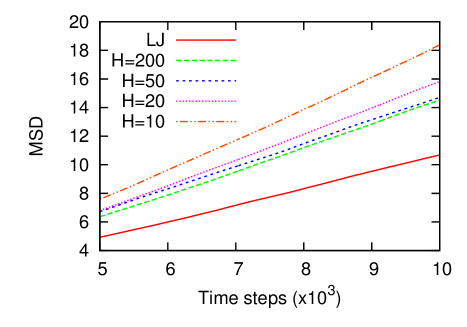
Figure 1 shows the time dependence of the MSD for various values of $H$ of the soft-core potential and for a LJ potential. For large values of $H$, the soft-core potential of (1) is qualitatively similar to $U_{LJ}(r)$. For all values of $H$, the dynamics of the system lead to normal diffusion ($\left<\Delta r^{2}\right>\sim t$). The simulation results indicate that the diffusion coefficient $D$ ($\left<\Delta r^{2}\right>=6Dt$) depends on the softness of the potential. The harder the short-range part the lower $D$ will be, as the collisions approach a hard-sphere interaction. The qualitative features of the VACF, RDF, energy and temperature obtained with $U_{SC}(r)$ resemble those of a simulation with a LJ potential. There are some differences in the computed observables and the RDF, for example, reflects that the soft core allows penetration. The positional structure, typical for a liquid, is still visible in the RDF. The most important aspect, however, is the ubiquitous presence of the Gaussian statistics in the self-diffusion properties.

3 Out-of-equilibrium simulation

We now turn to simulations under non-equilibrium conditions. Under equilibrium conditions, the energy is conserved and the temperature fluctuates mildly around a certain value. We introduce non-equilibrium conditions by driving the system and modifying the inter-particle interaction. This can be achieved by rescaling the radial distances in the soft-core interaction $U_{SC}(r)\rightarrow U_{SC}(\lambda r)$ with $\lambda<1$. This is equivalent to an effective increase of the size of the molecules. This allows the dynamics of the system to be changed dramatically, because particles that were attracting each other end up repelling each other due to the driven change in the inter-particle interaction range. As the imposed changes in the inter-particle interactions occur under conditions of constant density, the system develops regions of high energy density. Through the dynamics of the system, local energy surplus dissipates into sizeable kinetic energy and an increase in the temperature of the system is observed. Figure 2 shows the evolution of the temperature with time for a simulation that undergoes a rescaling of the soft-core interaction of the particles. It is clear that the driven change in the radius of the molecules has a large effect on the temperature. After rescaling the radial distances, it takes of the order of a few hundred time steps for the temperature to reach a new equilibrium value.

Figure 2: Temperature as a function of time for a simulation in which a radial rescaling with $\lambda=0.75$ takes place every 500 time steps. When the temperature reaches 50, the radii and the temperature are reset to their original value ($T_{init}=0.7$).

(a) SC(neq)

(b) LJ(neq)

(c) SC(eq)

(d) LJ(eq)

Figure 3: A typical spatial distribution of the potential energy changes $\Delta E_{pot}(\textbf{r}_{i})$ in one time step. We show the projection onto the $xy$-plane for $|z_{i}|\leq 0.5$ under conditions of (a) a soft-core potential just after rescaling with $\lambda=0.7$ (neq), (b) a LJ potential just after rescaling with $\lambda=0.7$ (neq), (c) a soft-core potential during equilibrium (eq), (d) a LJ potential during equilibrium (eq).

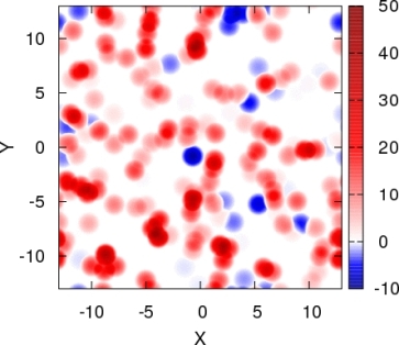
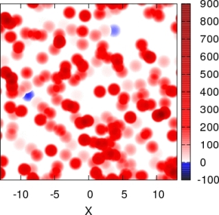
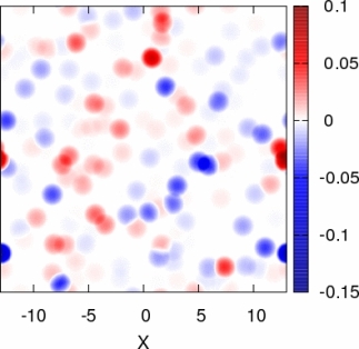
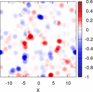
To illustrate the effect of the radial rescalings on the internal dynamics of the system, the potential energy fluctuation of the system during one simulation step is shown in figure 3. We consider results for $U_{LJ}(r)$ and $U_{SC}(r)$ under typical equilibrium conditions and a situation just after a radial rescaling. For every particle the difference in potential energy with respect to the previous configuration is shown

$$\Delta E_{pot}(\textbf{r}_{i})=\sum_{j\neq i}U\left(\textbf{r}_{ij}\left(t+\Delta t\right)\right)-U\left(\textbf{r}_{ij}\left(t\right)\right)\;.$$ (2)

The panels of figure 3 represent a projection of a slice ($\forall i:|z_{i}|\leq 0.5$) onto the $xy$-plane. Figure 3a indicates that through a sudden rescaling of the radial distances one creates regions in which the total amount of potential energy gain is much larger than the average value. Figure 3b shows that the hard core of $U_{LJ}(r)$ results in values of $\Delta E_{pot}$ as high as $800$, whereas this is not seen in figure 3a. With energy fluctuations of this size, the velocities of the particles attain values that are not compatible with a finite time-step. Figure 3c and figure 3d show a similar type of projection for typical equilibrium conditions. The scale of $\Delta E_{pot}$ is clearly much smaller than in the non-equilibrium situations of figures 3a and 3b.

The regular rescaling of the inter-particle distances drives the system’s thermodynamic properties such as the temperature and the energy away from equilibrium, i.e. mild fluctuations around a constant value. As a result, the simulation resembles conditions encountered in systems which display self-organized criticality (SOC) [23]. These systems are characterized by a driving and a relaxation mechanism. In our studies, the increase of the radius is the driving factor that injects potential energy at various positions in the system and the conversion from potential to kinetic energy is the relaxation mechanism. The balance between the injected and dissipated energy is linked through the local Newtonian dynamics that conserves total energy. Another characteristic feature of SOC is that the system must be driven slowly. For our purposes, this translates into changing $\lambda$ after sufficiently long time intervals. For a LJ-potential, the driven changes in the distance scale of the inter-particle interaction amount to very large potential energy changes (Figure 3b) that are not compatible with slowly driving the system.

As repeatedly increasing the radii is not an attractive option (because of the finite size of the simulation system), after some time we reset the system’s original temperature and particle radius. If the temperature exceeds a certain threshold, the radii are rescaled to their original value and the velocities are rescaled so that the starting temperature is restored, see figure 2.

4 Results

We identify the time intervals with a varying temperature in figure 2 as non-equilibrium conditions. Now, we study the self-diffusion properties of the liquid under those non-equilibrium conditions. For a single time-step, the mean, standard deviation and kurtosis of $P(\Delta x),P(\Delta y)$ and $P(\Delta z)$ are calculated. The standard deviation ($\sigma$) and kurtosis ($k$) are defined in the standard fashion,

$$\sigma(t) = \sqrt{\frac{1}{N}\sum_{i=1}^{N}(\Delta x_{i}(t)-\overline{\Delta x(t)})^{2}}$$ (3)

$$k(t) = \frac{\mu_{4}(t)}{\sigma^{4}(t)}-3,$$ (4)

with $\mu_{4}$ the fourth moment about the mean. This definition ensures that for a Gaussian distribution, the kurtosis vanishes.

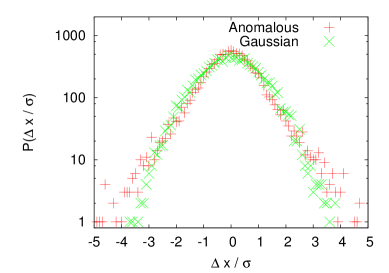
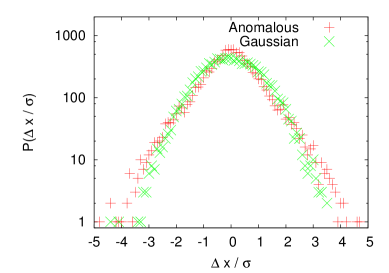
To normalise the width of the different distributions, the displacements are divided by the standard deviation of the distribution at some time instance. This normalisation enables one to compare the $P(\Delta x/\sigma)$ that are obtained at different times. Figure 4a compares $P(\Delta x/\sigma)$ for a typical equilibrium time instance with one obtained at a representative non-equilibrium time instance. Under non-equilibrium conditions, the tails of $P(\Delta x/\sigma)$ are considerably fatter than under equilibrium conditions. Moreover, a higher concentration of particles in the centre of the distribution is observed. These characteristics are typical for a leptokurtic distribution. The kurtosis of the out-of-equilibrium $P(\Delta x/\sigma)$ are larger than the typical noise level under equilibrium conditions.

We have found that after effectively enlarging the particles, anomalous characteristics can be found in the single time step displacement distributions $P(\Delta x/\sigma)$. After rescaling the interaction four times with $\lambda=0.75$ and 500 time steps between the different rescalings (sufficient to reach equilibrium again), we have obtained anomalous distributions in $P(\Delta x/\sigma)$.

(a)

(b)

(c)

(d)

Figure 4: $P(\Delta x/\sigma)$ for two typical equilibrium (Gaussian) and non-equilibrium (anomalous) situations with initial density $\rho=0.5$, temperature $T=0.7$. The upper panels are for $\lambda=0.7$ after four rescalings. The lower panels are for $\lambda=0.75$ after four rescalings. The right panels are a fit of $P(\Delta x/\sigma>1.5)$ with (5). The best fit parameters are $a=792$ and $b=0.14$ for the upper right panel and $a=628$ and $b=0.13$ for the lower right panel.

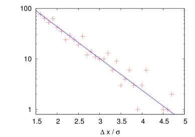
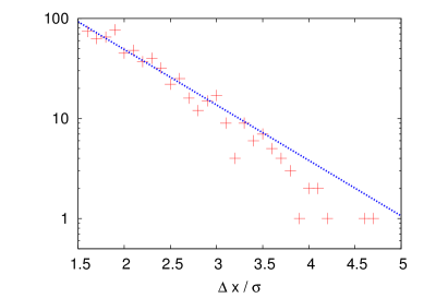
To establish the non-Gaussian shape of the tail of $P(\Delta x/\sigma)$ under non-equilibrium conditions, we have fitted it with an exponential:

$$P(\frac{\Delta x}{\sigma})=a\exp\left(-b\frac{\Delta x}{\sigma}\right),\qquad\left(\frac{\Delta x}{\sigma}>1.5\right).$$ (5)

As can be seen in figure 4b and 4d, the distributions are well fitted by (5). This result confirms that the $P(\Delta x/\sigma)$ have fatter tails than a Gaussian distribution.

(a)

(b)

Figure 5: Left: Summation of 50 ’anomalous’ and ’Gaussian’ distributions of P($\Delta x/\sigma$). Right: Normalized cumulative distribution of the sum of 50 ’anomalous’ and ’Gaussian’ distributions P($\Delta x/\sigma$).

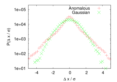
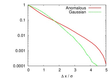
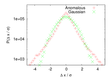
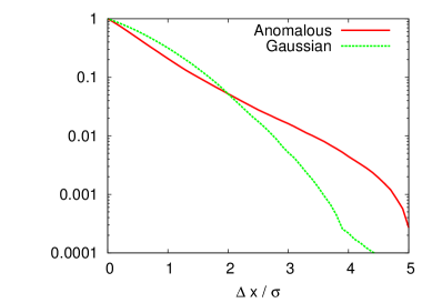
The distributions of figures 4a and 4c are obtained by taking data during one time step. Summing these distributions for different time steps results in better statistics. Figure 5a shows the result for P($\Delta x/\sigma$) after summation of 50 distributions during anomalous and normal (Gaussian) simulation conditions. Remark that $\frac{\left|\Delta x\right|}{\sigma}>4$ events are one order of magnitude more likely under anomalous (non-equilibrium) conditions than under Gaussian (equilibrium) conditions. We find a fair amount of $5\sigma$ events and some rare $8\sigma$ events. The normalized cumulative distribution of figure 5 clearly illustrates that the self-diffusion properties of the liquid are distinctive during the non-equilibrium and equilibrium periods of the simulation. In non-equilibrium conditions, small $\Delta x/\sigma$ are more likely, medium $\Delta x/\sigma$ less likely and large $\Delta x/\sigma$ far more likely.

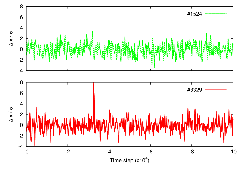
We now wish to study the trajectories of the individual particles during the complete simulation that alternates equilibrium with non-equilibrium conditions. To this end, we selected two particles: particle $\#1524$ for which $|\Delta x/\sigma|$ does not exceed $5$ during the simulation (since this limit isn’t attainable in a Gaussian simulation regime) and particle $\#3329$ for which this is not the case. Figure 6 illustrates that the random character of the trajectories for both particles is maintained over the simulation time.

Figure 6: Projection on the $xy$-plane of $\sum_{t}\;\Delta\textbf{r}(t)/\sigma(t)$ of particles $\#1524$ and $\#3329$ during a simulation of $100000$ time-steps.

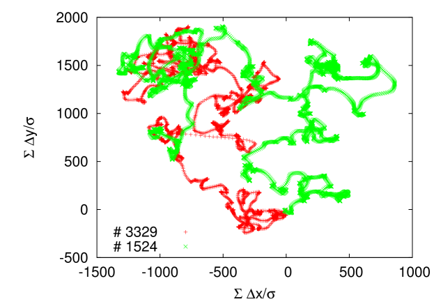
Figure 7 shows $\Delta x/\sigma$ as a function of time for these particles. The ”anomalous” behaviour of particle $\#3329$ is confined to the time period $32000$ - $33000$. By contrast, no anomalous behaviour is discernible in the behaviour of particle $\#1524$.

Figure 7: Single time step displacements ($\Delta x(t)/\sigma(t)$) of particles $\#1524$ and $\#3329$ during a simulation of $100000$ time steps.

To establish the robustness of our technique to generate conditions of anomalous self-diffusion in a mono-atomic liquid, we have investigated its dependence on the parameters of the simulations. The non-equilibrium conditions are determined by the size of the rescaling parameter $\lambda$ and the time intervals between two subsequent radial rescalings. During a simulation of $100000$ time-steps, the system goes through different periods of non-equilibrium conditions. The kurtosis of P($\Delta x/\sigma$) is computed for every time-step and the maximal kurtosis is saved for every set of parameters. In figure 8 the maximum kurtosis of the simulation is plotted as a function of $\frac{1}{\lambda}$ and the time interval between two rescalings. The time intervals are chosen between $100$ and $1500$ time-steps, since equilibrium is always reached after $1500$ time-steps. $\lambda$ is confined to $1<1/\lambda<1.4$, which means that the density change in one step is limited to $1<\Delta\rho<2.7$. Figure 8 clearly shows that the anomalous character of $P(\Delta x/\sigma)$ remains present independent of the rescaling parameters. The time interval between two subsequent rescalings ($\tau$) has only a minor influence on the maximal kurtosis ($k_{max}$). The adopted value of $\lambda$, on the other hand, has a larger influence on $k_{max}$, but the anomalous characteristics are present in the entire $\lambda$ interval.

The same robustness applies to variations in the initial density and temperature of the system, provided that they generate a system in the liquid phase. The short range order and particle mobility typical for a liquid are necessary conditions. They generate the required balance between mobility and interaction, allowing the system to dissipate the potential energy surplus after being driven.

Figure 8: Maximal kurtosis ($k_{max}$) of a simulation as a function of the rescaling parameter $\frac{1}{\lambda}$ and the time interval $\tau$ between two subsequent rescalings.

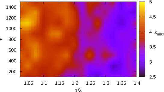
The robustness of the anomalous character of the self-diffusion properties under non-equilibrium conditions is a very useful result. It indicates that the qualitative features of the self-diffusion properties of the system are rather insensitive to the two parameters ($\lambda$ and $\tau$) that characterise the non-equilibrium behaviour. As a consequence, we can ascertain that it is the internal dynamics of the system that causes the non-Gaussian properties of $P(\Delta x/\sigma)$.

We have also tested the robustness of our results to changes in the potential. To this end, we have performed simulations with the following potential: a LJ for $r_{ij}>0.9$ and a polynomial $ar^{6}+b$ for $r_{ij}<0.9$ [24]. This potential has the long-range LJ properties and a soft core. We have obtained non-Gaussian distributions almost identical to those obtained with $U_{SC}(r)$.

A further test of the robustness of our technique can be done in dimensions other than three. In two dimensions we obtain inherent anomalous self-diffusion of the system, as expected [5, 13]. Figure 9 shows the result of a simulation in four dimensions. We have used the same technique as the one adopted for the 3D results of Figure 5. From figure 9 it is clear that during the non-equilibrium time periods the self-diffusive properties are non-Gaussian. This provides further evidence for the robustness of the proposed technique.

(a)

(b)

Figure 9: $P(\Delta x/\sigma)$ for a four-dimensional simulation with $4375$ particles, summed over 350 time instances, for two typical equilibrium (Gaussian) and non-equilibrium (anomalous) situations, with $\lambda=0.8$ and $\tau=1000$.

5 Conclusion

In summary, we have presented a computational method, based on out-of-equilibrium MD simulations with a soft-core potential, that generates dynamical conditions of anomalous diffusion for the distribution of the one-dimensional displacements of the particles. This behaviour arises because the driving mechanism, i.e. the potential energy artificially injected into the system by increasing the radius of the particles, generates regions of increased potential energy. The dissipation of this potential energy under conditions of constant energy results in a small amount of very fast particles. For a broad range of the parameters involved, our technique generates anomalous diffusion in the simulation. In this way we have created a simple and elegant method to achieve anomalous self-diffusion in an interacting system. This emergence of global behaviour that cannot be determined from local properties is also a property of self-organized criticality, to which our model bears similarities.

References

- [1] A. Einstein, Ann. Phys. 17, 549 (1905).
- [2] P. Lévy, Théorie de l’addition des variables aléatoires, Gauthier-Villars (1954).
- [3] R. N. Mantegna, Phys. Rev. E 49, 4677 (1994).
- [4] R. N. Mantegna and H. E. Stanley, Phys. Rev. Lett. 73, 2946 (1994).
- [5] J. Klafter and I. M. Sokolov, Phys. World 18, 29 (2005).
- [6] J.-P. Bouchaud and A. Georges, Phys. Rep. 195, 127 (1990).
- [7] B. Mandelbrot, J. Business 36, 394 (1963).
- [8] R. Mantegna and H. Stanley, Nature 376, 46 (1995).
- [9] K. Kiyono, Z. Struzik, and Y. Yamamoto, Phys. Rev. Lett. 96, 068701 (2006).
- [10] G. Ramos-Fernández et al, Behav. Ecol. Sociobiol. 55, 223 (2004).
- [11] I. Wong et al, Phys. Rev. Lett. 92, 178101 (2004).
- [12] G. S. Janes and R. S. Lowder, Phys. Fluids 9, 1115 (1966).
- [13] B. Liu and J. Goree, Phys. Rev. E 75, 016405 (2007).
- [14] S. Havlin and D. Ben-Avraham, Adv. Phys. 51, 187 (2002).
- [15] M. Schmiedeberg and H. Stark, Phys. Rev. E 73, 031113 (2006).
- [16] R. Juhász, Phys. Rev. E 78, 066106 (2008).
- [17] A. Majda and P. Kramer, Phys. Rep. 314, 237 (1999).
- [18] B. Alder and T. Wainwright, Phys. Rev. A 1, 18 (1970).
- [19] G. Kresse and J. Hafner, Phys. Rev. B 47, 558 (1993).
- [20] M. Mondello and G. Grest, J. Chem. Phys. 106, 9327 (1997).
- [21] P. Crozier et al, and D. Busath, Phys. Rev. Lett. 86, 2467 (2001).
- [22] G. Franzese, J. Mol. Liq. 136, 267 (2007).
- [23] P. Bak, How nature works: The science of self-organized criticality (Copernicus, New York, 1996).
- [24] K. Tappura, M. Lahtela-Kakkonen, and O. Teleman, J. Comput. Chem. 21, 388 (2000).