Housing Market Microstructure

Abstract

In this article, we develop a model for the evolution of real estate prices. A wide range of inputs, including stochastic interest rates and changing demands for the asset, are considered. Maximizing their expected utility, home owners make optimal sale decisions given these changing market conditions. Using these optimal sale decisions, we simulate the implied evolution of housing prices providing insights into the recent subprime lending crisis.

Keywords: Real estate market; Price evolution; Optimal waiting time

1 Introduction

The recent turmoil in financial markets triggered by defaults on subprime mortgages demonstrates that home prices are largely driven by buyers’ demands. Indeed, in the early 2000s, house prices rose to record levels due to the high demand for mortgages with easy credit. The left-side graph in Figure 1 plots the Case-Shiller Composite-20 house-price index, which shows that the prices peaked in 2006, were stable for a while, and subsequently decreased. Figure 1 documents the level of mortgage rates and home inventories during the same period. During the house price appreciation cycle (2000-2005), there is a sharp decrease in mortgage rates and a slight increase in home inventories. Low mortgage rates result in an increased demand for mortgages and housing. In contrast, the period with decreasing house prices (2006-2007) corresponds to a sharp increase in mortgage rates and home inventories. In this paper, we propose a mathematical model to explain the relation between house prices and buyers’ demands using a market microstructure perspective. We consider both market and personal shocks, and we analyze how these shocks affect the home owner’s optimal sale decision and the resulting sale process. Our model can also be used to forecast the future price evolution of house prices under different interest rate and demand scenarios.

Our paper is related to two topics in the literature: the optimal waiting time (OWT) and the home sale price evolution. Time-on-the-market (TOM), time-to-sale, optimal marketing time, and selling time are frequently used terms that have similar connotations to OWT even though their exact economic definitions may differ . The existing literature in this area is mostly empirical focusing on the sign of the correlation between the length of TOM and the resulting sale price. Cubbin (1974) builds an econometric model to explain the relationship between the list price and selling time using data from the Coventry housing market between 1968 and 1970. Cubbin finds that the higher the list price, the shorter the selling time. Miller (1978) cannot confirm Cubbin’s conclusion using 83 sales from Columbus, Ohio. Miller’s empirical study does not confirm the existence of an optimal selling time. Kalra, Chan and Lai (1997) analyze 644 single-family house sales records in the Fargo-Moorhead metropolitan area to conclude that TOM and sale price are positively related. Genesove and Mayer (1998) conclude from a study of the Boston condominium market that owners’ with a high loan-to-value ratio have a longer time on the market and sell properties for higher prices. Taylor (1999) studies the theoretical relationship between TOM and property quality. Knight (2002) examines how changes in the list price impact the resulting TOM and sale price. In contrast, our paper does not explicitly test the relationship between expected TOM and our model’s parameters, but rather we investigate the relationship between OWT, list, and reservation prices. In addition, we also examine the relationships between OWT and interest rates, and order arrival and withdrawal intensities - which are not well-studied in the literature.

$\begin{array}[]{c@{\hspace{-0.5cm}}c@{\hspace{-0.5cm}}c}\includegraphics[width=170.71652pt]{cs}&\includegraphics[width=170.71652pt]{rate}&\includegraphics[width=170.71652pt]{inventory}\\ \mbox{\footnotesize Case-Shiller Composite-20 index}&\mbox{\footnotesize 30-year fixed mortgage rate}&\mbox{\footnotesize Existing home inventory}\end{array}$

Figure 1: With the housing meltdown, the house-price index is falling, existing inventory is piling up and current mortgage rate is significantly higher than its trough.

Many of the models studying TOM are based on information theory with search and matching models. With their corresponding optimal stopping rules, these models have been used to explain the behavior of buyers and sellers. Buyers search until the marginal benefit of continued search is equal to marginal cost, and similarly, sellers equate the marginal benefit to the marginal cost of locating a bidder for their property. Haurin (1988) applies search theory to investigate the relationship between the distribution of offers and the duration of marketing time. His empirical study concludes that as the variance of the offer distribution increases, the expected marketing time lengthens. Sarr (1988) examines the optimal list price adjustment under demand uncertainty. Wheaton (1990) investigates the role of vacancy rates in determining TOM, the reservation, and sale prices. He finds that greater vacancy increases selling time, lowers the seller’s reservation price, and ultimately leads to lower market prices. Although we do not study vacancy rates in our model, our findings are similiar to Wheaton’s (1990) for a seller with a low reservation price. In this case, OWT increases and the seller expects less from the transaction. Forgey, Rutherford and Springer incorporate liquidity into a search model. Using data from $3358$ single-family housing transactions, they conclude that an optimal marketing period exists and properties with higher liquidity sell at a higher price. Yavas (1992), Krainer and LeRoy (2002) and Williams (1995) also apply search and matching theory to analyze the sale prices of illiquid assets. Our paper differs from these papers in our modeling approach. We do not use a search and matching model, but instead employ a market microstructure model. We incorporate the reservation price, the list price, the distribution of offers, withdrawal rates for buyers’ offers, and deterministic and stochastic interest rates. The seller’s motivation is captured by a time impatient utility function. We find the optimal selling time that maximizes the seller’s expected utility. OWT in our model is set at the beginning of the sales process. Optimal timing of investment has been previously studied in the case of known asset price dynamics by Grenadier and Wang (2005) and Evans, Henderson and Hobson (2007). In our paper, we do not study the risk associated with the waiting period - which is well-documented by Lin and Vandell (2007).

Real estate market price evolutions are considered in the second part of our paper. The existing literature on price evolutions relies mostly on econometric models. Since the housing market is heterogeneous in the qualities of the properties, most of the existing literature is devoted to developing statistical techniques to overcome this heterogeneity by forming price indices for geographical areas, see Bailey, Muth and Nourse (1963), Case K. and Shiller (1987), Case K. and Shiller (1990), Case B. and Quigley (1991), and Poterba, Weill and Shiller (1991), Goetzmann and Peng (2006), and McMillen and Thorsnes (2006). Another stream of literature uses equilibrium theory to estimate house price dynamics. Stein (1995) explains the large swings in prices by introducing an equilibrium model with a down-payment effect. Similarly, Ortalo-Magne and Rady (2006) present a recursive equilibrium model that accounts for income shocks and credit constraints. Capozza, Hendershott and Mack (2004) use mean reversion and serial correlation to explain equilibrium house price dynamics. Our model differs from this literature. We use the derived analytics from our OWT framework and extend it to multiple selling periods to determine the price evolution. Given the linkage between the seller and the buyer (e.g., the transaction price becomes the reservation price of the buyer when he posts the property for sale), we construct a property price evolution by tracking the expected sale price in the selling process. Our OWT framework enables us to examine housing price movements under different interest rate and demand scenarios. We model the timing of the decision of sale for each owner with random income and personal shocks. Simulation shows that the fluctuation in housing prices are driven by interest rates, demand for the asset, and reservation prices.

This paper is organized as follow. Section 2 introduces the model within the OWT framework. We start with an auxiliary model, extend it to more realistic cases, and analyze the comparative statistics of OWT with respect to model parameters. Section 3 applies our model to the price evolution in the real estate market. Section 4 provides a simulation and reflects on the subprime lending crisis. Finally, Section 5 concludes.

2 The Model

Sellers of illiquid real assets often face a difficult decision regarding how long they should keep the asset on the market if they do not receive any offers matching the list price. If the asset is highly desirable, the seller might remain undecided even in the case of receiving an offer at the list price. He may wait an additional amount of time in hopes of receiving an offer even greater than the list price. If he chooses to wait longer, he may lose the current offer. As this discussion implies, the determination of the waiting time is complicated when there is a mutual decision process between the seller and the buyer. This section analyzes the optimal amount of time that a seller should wait in this mutual decision process to maximize his expected payoff.

We consider two cases in our optimal waiting time (OWT) analysis. In the first, the seller does not specify his final list price and accepts the highest available offer exceeding his reservation price, $R$, at the end of the OWT. In the second, he publicly announces the list price, $L$, and keeps the reservation price $R$ private. He sells the asset if he receives an offer greater than $L$; otherwise, he waits until the end of the OWT and then chooses the best offer greater than $R$. We assume that buyers make offers at random times with random magnitudes. Buyers may also withdraw their offers according to a known random process.

We begin with the mathematical formulation of an auxiliary model. We provide the details of the derivation for this auxiliary model in the appendix. We then consider the two cases: (i) where the reservation and list prices are private information, and (ii) where the seller announces a pre-determined list price.

2.1 The Auxiliary Model

In the auxiliary model, the seller’s reservation price, denoted $p_{\min}$, is public information (i.e., all of the offers that the seller receives are higher than $p_{\min}$). We assume that the arrival times of the buyers’ offers follow a one-dimensional Poisson point process with parameter $\lambda$, and the magnitudes of their offers are uniformly distributed with $U(p_{\min},p_{\max})$ where $p_{\max}$ is finite. After making an offer, a buyer may withdraw his offer. The time to withdrawal is assumed to follow an exponential distribution with parameter $\mu$. Lastly, interest rates are assumed constant and equal to $r$.

The seller maximizes their discounted expected payoff with respect to the waiting time, $T$. Let the expected discounted payoff function be denoted by $u(T,\lambda,\mu,p_{\min},p_{\max},r)$. The following lemma characterizes this quantity.

Lemma 2.1

$$u(T,\lambda,\mu,p_{\min},p_{\max},r) =\left(-\frac{g(T,\lambda,\mu,r)(p_{\max}-p_{\min})}{(1-f(T,\mu))^{2}}\right)\times$$

$$\left(f(T,\mu)e^{\lambda Tf(T,\mu)}-\frac{1}{\lambda T}(e^{\lambda Tf(T,\mu)}-1)-e^{\lambda Tf(T,\mu)}+\frac{1}{\lambda T}(e^{\lambda T}-1)\right)$$

$$+\frac{p_{\max}g(T,\lambda,\mu,r)(e^{\lambda T}-e^{\lambda Tf(T,\mu)})}{1-f(T,\mu)}$$ (2.1)

where $f(T,\mu)=1-\frac{1}{\mu T}(1-e^{-\mu T})$ and $g(T,\lambda,\mu,r)=(1-f(T,\mu))e^{-rT}e^{-\lambda T}$.

Proof.    See Appendix A. $\blacksquare$

This lemma is used in the following two cases.

2.2 No List Price

In this case the seller’s reservation price, $R$, is private information. The seller does not post a list price, and considers all offers until the end of the waiting time. Here the seller has a minimum price for a sale, but doesn’t limit the upside payoff.

Using the thinning principle for Poisson processes, Resnick (1992), the expected discounted payoff, $v(T,\lambda,\mu,R,p_{\min},p_{\max},r)$, can be computed as in the following corollary.

Corollary 2.1

$v(T,\lambda,\mu,R,p_{\min},p_{\max},r)=u(T,\lambda_{\text{thinned}},\mu,R,p_{\max},r)$ where $\lambda_{\text{thinned}}=\lambda\frac{p_{\max}-R}{p_{\max}-p_{\min}}$.

Figure 2: Expected discounted payoff in the case without a list price.

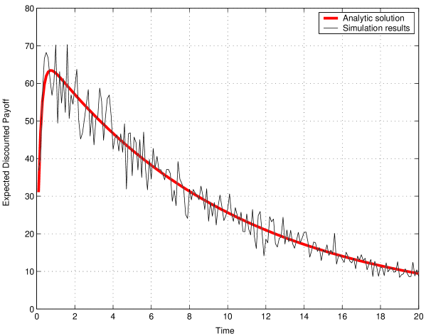
Figure 2 plots the expected discounted payoff as in Corollary 2.1. The values of the parameters used in this figure are contained in the appendix. The expected discounted payoff equals zero at $T=0$, increases to a maximum value, and then starts to decrease. This plot shows that there is an optimal waiting time.

2.3 Public List Price

In this case the seller announces a list price, $L$, and still has a private reservation price, $R$. This case can be simplified by dividing the payoff function into two regions. From Corollary 2.1, if the seller does not receive any offers higher than $L$, the payoff becomes $u(T,\lambda\frac{L-R}{p_{\max}-p_{\min}},\mu,R,L,r)$. The remaining region is when offers higher than $L$ are received. The payoff function, $w(T,\lambda,\mu,R,L,p_{\min},p_{\max},r)$, is obtained by considering these two regions.

Theorem 2.1

$$w(T,\lambda,\mu,R,L,p_{\min},p_{\max},r) =\left(1-e^{-\lambda Ty}\right)\left(\frac{p_{\max}+L}{2}\right)\left(\frac{\lambda y}{\lambda y+r}\right)$$

$$\qquad+e^{-\lambda Ty}u(T,\lambda x,\mu,R,L,r)$$ (2.2)

where $x=\frac{L-R}{p_{\max}-p_{\min}}$ and $y=\frac{p_{\max}-L}{p_{\max}-p_{\min}}$.

Proof.    If the seller does not receive any offer higher than $L$, the payoff equals $u(T,\lambda\ x,\mu,R,L,r)$. Given that there is an offer higher than $L$, our payoff equals $\frac{p_{\max}+L}{2}\mathbb{E}\left[e^{-r\beta}\right]$ where $\beta$ is a random variable representing the arrival time of the first offer greater than $L$. If $y=\frac{p_{\max}-L}{p_{\max}-p_{\min}}$, then $\mathbb{E}\left[e^{-r\beta}\right]$ equals the moment-generating function of an exponential random variable with parameter $\lambda y$. Thus, $\mathbb{E}\left[e^{-r\beta}\right]=\frac{\lambda y}{\lambda y+r}$.  To find the resulting expected payoff, we only need the probability of receiving an offer greater than $L$, which equals $\left(1-e^{-\lambda Ty}\right)$. As a result, our expected payoff function is the sum of these two parts multiplied by their corresponding probabilities. $\blacksquare$

Figure 3: Expected discounted payoff in the case with an announced list price

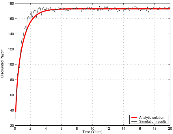
Figure 3 graphs the expected discounted payoff with respect to the waiting time for a public list price. The values of the parameters used in this graph are contained in the appendix. Note that the expected payoff function is strictly increasing in $T$ with an asymptote:

$$\lim_{T\rightarrow\infty}w(T,\lambda,\mu,R,L,p_{\min},p_{\max},r)=\left(\frac{p_{\max}+L}{2}\right)\left(\frac{\lambda y}{\lambda y+r}\right).$$ (2.3)

When $T$ increases, the payoff function is dominated by the region where the seller receives an offer greater than $L$. Unlike the first model, the asymptotic payoff is not a function of the waiting time, $T$, and therefore, does not diminish with respect to $T$. By setting a longer waiting time, the seller can almost surely get an offer greater than $L$ (and because the discount factor, $\mathbb{E}\left[e^{-r\beta}\right]$, does not depend on $T$.) This is due to the properties of the exponential distribution for the first offer greater than $L$. This figure does not imply that the seller waits an infinite amount of time to sell the asset. Rather, it only implies that the seller makes a conservative estimate of the maximum waiting time before the sale process starts.

The reason why the expected discounted payoff is increasing in $T$ is because there is no specific utility function associated with the seller’s motivation to sell the asset (see Glower, Haurin and Hendershott (1998) who show that the seller’s motivation is a significant factor in determining the selling time and the sale price). We can introduce this utility based sales motivation via a utility function, $\mathcal{U(.)}$, defined as follows.

Definition 2.1

$\mathcal{U}(D,T)=De^{-\gamma T}$ where $D$ is the discounted payoff, $T$ is the waiting time, and $\gamma\geq 0$ is a time impatience parameter.

As the time impatient parameter $\gamma$ increases, the seller is more motivated to sell the asset. This selling motivation enables the model to incorporate different individuals, who have different sale processes even under the same market conditions. With this assumption, the expected utility function, $z(.)$, can be written as follows.

Corollary 2.2

$$z(T,\lambda,\mu,R,L,p_{\min},p_{\max},r,\gamma) =\mathbb{E}\Big{[}\mathcal{U(.)}\Big{]}$$ (2.4)

$$=e^{-\gamma T}w(T,\lambda,\mu,R,L,p_{\min},p_{\max},r)$$ (2.5)

Figure 4: Expected utility in the case of an announced list price

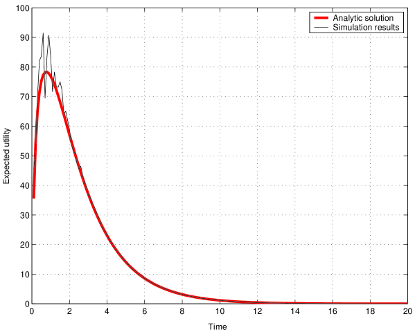
Figure 4 plots the expected utility with respect to the waiting time in the case of a public list price. The parameter values used in this graph are contained in the appendix.

2.4 An Analysis of OWT

This section defines the OWT and analyzes its comparative statistics with respect to the model’s parameters. We use the public list price case of Section 2.3 as our underlying model.

Definition 2.2

Let $T^{\ast}$ denote the OWT that maximizes expected utility. Then,

$$T^{\ast}=\arg{\max{\{T\geq 0:z(T,\lambda,\mu,R,L,p_{\min},p_{\max},r,\gamma)\}}}.$$ (2.6)

Since the expected utility function is continuous and its first derivative has a unique sign change from positive to negative, a global maximum exists. We plot $T^{\ast}$ as a function of model’s parameters in Figures 5 through 7. The parameter values used in the graphs are contained in the appendix.

$\begin{array}[]{c@{\hspace{.5cm}}c}\includegraphics[width=227.62204pt]{lambda_r}\hfil\hskip 14.22636pt&\includegraphics[width=227.62204pt]{mu_r}\\ \hfil\hskip 14.22636pt&\end{array}$

Figure 5: Optimal waiting time as a function of arrival intensity and interest rate (left) and optimal waiting time as a function of withdrawal intensity and interest rate (right)

The graph on the left side of Figure 5 shows the change in $T^{\ast}$ with respect to the arrival intensity of offers, $\lambda$, and interest rates $r$. As $\lambda$ increases, the seller chooses a smaller waiting time because he expects to get sufficiently many offers and, thus, he avoids a large utility loss from waiting longer. This graph illustrates this point with a decreasing concave-up function when interest rates are low. However, when interest rates are high, we see that $T^{\ast}$ actually increases when $\lambda$ is small and increasing. This implies that in this region, the amount of additional offers created by higher demand is worth the wait.

The graph on the right-side graph of Figure 5 shows the change in $T^{\ast}$ with respect to the withdrawal intensity of the buyers, $\mu$, and interest rates $r$. As $\mu$ increases, the seller chooses a longer waiting time because he wants to increase the number of offers, as in the case of the increasing arrival intensity. Figure 5 shows that, when interest rates are high, there is a constant optimal waiting time. In this circumstance, since the discount rate is high, small changes in the withdrawal intensity do not affect $T^{\ast}$.

Both of these graphs show that interest rates are indirectly proportional with $T^{\ast}$. This is intuitive because the seller does not want to wait long in a high interest rate environment.

Figure 6: Optimal waiting time as a function of arrival intensity and withdrawal intensity

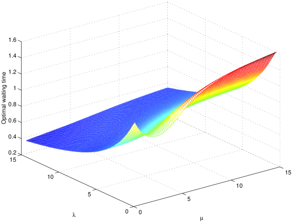
Figure 6 illustrates that the intensities of offer arrivals $\lambda$ and offer withdrawals $\mu$ do not always create the opposite impact on $T^{\ast}$. For small values of $\lambda$ and $\mu$, $T^{\ast}$ increases when they both rise above a certain threshold. Only after this threshold do they begin to create the opposite effect.

The left-side of Figure 7 shows the change in $T^{\ast}$ with respect to the list price and interest rates. When the list price increases, the OWT increases. However, as Figure 7 illustrates, if our list price is already high, increasing the list price further diminishes the probability of receiving an offer greater than this new value and, thus, there is no incentive to wait longer.

The right-side of Figure 7 shows the change in $T^{\ast}$ with respect to the reservation price and interest rates. As $R$ increases, the seller waits longer because, using the thinning principle in Poisson processes, this case implies a decreasing $\lambda$. As we have seen earlier, decreasing the arrival intensity results in a larger $T^{\ast}$.

$\begin{array}[]{c@{\hspace{.5cm}}c}\includegraphics[width=227.62204pt]{S_r}\hfil\hskip 14.22636pt&\includegraphics[width=227.62204pt]{R_r}\\ \hfil\hskip 14.22636pt&\end{array}$

Figure 7: Optimal waiting time as a function of list price and interest rate (left) and optimal waiting time as a function of reservation price and interest rate (right)

3 Modeling Real Estate Price Evolutions

The previous sections of the paper characterized the optimal waiting time when selling an illiquid asset. The remainder of the paper studies the time evolution of real estate sale prices in a market where sellers maximize their payoffs by considering the optimal waiting time.

3.1 Stochastic Demand and Interest Rates

The real estate market price evolution is strongly affected by changes in the broader economy such as recessionary or expansionary cycles and by interest rates shocks. In our model, we model the recessionary and expansionary cycles with a stochastic demand, $\lambda(t)$. The demand, $\lambda(t)$, will be a function of interest rates, $r(t)$, and the announced list prices, $L(t)$, i.e.

$$\lambda(t)=g\big{(}r(t),L(t)\big{)}$$ (3.7)

where $r(t)$ is stochastic and $L(t)$ is non-random for the seller.

It is assumed that $L(t)$ is non-increasing with $L(t)\geq R>0$ for all $t\geq 0$, where $R$ is the seller’s reservation price. Offers arrive according to a non-homogenous Poisson process with stochastic arrival intensity, $\lambda(t)$. Let $\mathcal{F}_{t}$ be the $\sigma$-algebra generated by $\{r(s)\}_{0\leq s\leq t}$, and $N(t)$ be the number of arrivals in $[0,t]$. Then,

$$\mathbb{P}\{N(t)=n\} = \mathbb{E}\Big{[}\Lambda(t)^{n}\frac{\exp(-\Lambda(t))}{n!}\Big{]},\mbox{ and}$$

$$\mathbb{P}\{N(t)=n|\mathcal{F}_{t}\} = \Lambda(t)^{n}\frac{\exp(-\Lambda(t))}{n!}$$ (3.8)

where $\Lambda(t)=\int_{0}^{t}\lambda(s)$d$s$.

Offers’ values come from an independent distribution, $F_{\xi}$ with density $f_{\xi}$, where $\xi$ represents the intensity of a generic offer. $\xi_{i}$ and $A_{i}$, $i\geq 1$, represent the intensity and the arrival time of the $i$th offer, respectively. Given $\mathcal{F}_{t}$ and the number of offers in $[0,t]$, offer arrival times are independently distributed over $[0,t]$ with conditional density

$$f_{A|\{\mathcal{F}_{t},N(t)=n\}}(a)=\frac{\lambda(a)}{\Lambda(t)}.$$

After an offer arrives, it is withdrawn after a random time with continuous distribution function $F_{\tau}$, where $\tau$ is the withdrawal time. It is not hard, however, to extend the analysis to more general offer withdrawal time distributions. We let $\tau_{i}$, for $i\geq 1$, represents the withdrawal time of the $i$th offer. All $\tau_{i}$’s are assumed to be independent from one another.

Without loss of generality, we set $\xi_{0}=A_{0}=\tau_{0}=0$. Let $\beta$ be the arrival time of the first offer greater than the list price. Then,

$$\beta=\inf\{A_{i}:\xi_{i}\geq L(A_{i}),i\geq 1\}.$$

We prove three theorems characterizing the expected payoff to the seller. In the first case, the seller announces a time-dependent list price. In this case, the asset is sold whenever there is an offer greater than the ask price. This is the most general case containing the others as subcases. In the second case, the list price of the asset does not change with time. Finally, in the third case, the seller does not announce a list price. He waits an optimal amount of time and then chooses the best available offer greater than the reservation price.

For the first case, the discounted payoff function, $X(t)$, at time $t$ is:

$$X(t) = \exp\Big{(}-\int_{0}^{t}r(s)ds\Big{)}\cdot\Big{(}\max_{0\leq i\leq N(t)}\xi_{i}\cdot 1\!\!1_{\{\xi_{i}\geq R\}}\cdot 1\!\!1_{\{\tau_{i}\geq t-A_{i}\}}\Big{)}\cdot 1\!\!1_{\{\beta>t\}}$$ (3.9)

$$+ \exp\Big{(}-\int_{0}^{\beta}r(s)ds\Big{)}\xi_{i(\beta)}1\!\!1_{\{\beta\leq t\}}$$

where $\xi_{i(\beta)}$ is the offer value at $\beta$. The first term in (3.9) accounts for the situation where all offers until time $t$ are smaller than the list price. The second term corresponds to the situation where there is an offer price greater than the list price before time $t$. We have the following theorem for the expected discounted payoff at time $t$.

Theorem 3.1

Let $P(t)=\mathbb{E}[X(t)]$ and $P(t|\mathcal{F}_{t})=\mathbb{E}[X(t)|\mathcal{F}_{t}]$. Then, $P(t)=\mathbb{E}[P(t|\mathcal{F}_{t})]$, and

$$P(t|\mathcal{F}_{t}) = \mathrm{e}^{-\int_{0}^{t}r(s)\mathrm{d}s}\mathrm{e}^{\Lambda(t)(\varphi(t)-1)}\Big{(}L_{0}-\int_{0}^{L_{0}}\mathrm{e}^{-\Lambda(t)\psi(t,y)}\mathrm{d}y\Big{)}$$ (3.10)

$$+ \big{(}1-\mathrm{e}^{\Lambda(t)(\varphi(t)-1)}\big{)}\int_{0}^{t}\int_{L(a)}^{\infty}\frac{\lambda(a)\exp\big{(}-\int_{0}^{a}r(s)\mathrm{d}s\big{)}}{\Lambda(t)\big{(}1-F_{\xi}\big{(}L(a)\big{)}\big{)}}f_{\xi}(x)x\mathrm{d}x\mathrm{d}a$$

where $\psi(t,y)=\frac{1}{\Lambda(t)}\int_{0}^{t}\lambda(a)\Big{(}1-F_{\tau}(t-a)\Big{)}\Big{(}F_{\xi}\big{(}L(a)\vee y\big{)}-F_{\xi}\big{(}R\vee y\big{)}\Big{)}\mathrm{d}a$ and $\varphi(t)=\frac{1}{\Lambda(t)}\int_{0}^{t}\lambda(a)F_{\xi}\big{(}L(a)\big{)}\mathrm{d}a$.

Proof.    See Appendix B. $\blacksquare$

The difficulty in proving Theorem 3.1 is that a changing list price introduces a coupling between the offer intensity and the arrival time.

In the second case, we assume that $L(t)$ is a constant. Here, the seller’s payoff can also be written exactly as in (3.9). Theorem 3.2 gives us the seller’s expected payoff at time $t$ for this case. We do not provide a proof because it is similar to that of Theorem 3.1.

Theorem 3.2

Let $P(t)=\mathbb{E}[X(t)]$ and $P(t|\mathcal{F}_{t})=\mathbb{E}[X(t)|\mathcal{F}_{t}]$. If $L(t)=L\geq R>0$ is constant, then $P(t)=\mathbb{E}\big{[}P(t|\mathcal{F}_{t})\big{]}$ and

$$P(t|\mathcal{F}_{t}) = \mathrm{e}^{-\int_{0}^{t}r(s)\mathrm{d}s}\mathrm{e}^{\Lambda(t)(F_{\xi}(L)-1)}\Big{(}L-\int_{0}^{L}\mathrm{e}^{-\Lambda(t)\psi(t,y)}\mathrm{d}y\Big{)}$$ (3.11)

$$+ \big{(}1-\mathrm{e}^{\Lambda(t)(F_{\xi}(L)-1)}\big{)}\int_{0}^{t}\int_{L(a)}^{\infty}\frac{\lambda(a)\exp\big{(}-\int_{0}^{a}r(s)\mathrm{d}s\big{)}}{\Lambda(t)\big{(}1-F_{\xi}\big{(}L(a)\big{)}\big{)}}f_{\xi}(x)x\mathrm{d}x\mathrm{d}a$$

where $\psi(t,y)=\big{(}F_{\xi}(L\vee y)-F_{\xi}(R\vee y)\big{)}\big{(}1-\frac{1}{\Lambda(t)}\int_{0}^{t}\lambda(a)F_{\tau}(t-a)\mathrm{d}a\big{)}$.

Finally, in the third case, the seller does not announce a list price. In this case, his payoff process at time $t$ can be written as

$$X(t)=\exp\Big{(}-\int_{0}^{t}r(s)ds\Big{)}\cdot\Big{(}\max_{0\leq i\leq N(t)}\xi_{i}\cdot 1\!\!1_{\{\xi_{i}\geq R\}}\cdot 1\!\!1_{\{\tau_{i}\geq t-A_{i}\}}\Big{)}.$$ (3.12)

The simplicity of (3.12) compared to (3.9) results in a simplification in the expected payoff formula at time $t$, which is given in Theorem 3.3. Again, we do not provide a proof because it is similar to the proof of Theorem 3.1.

Theorem 3.3

Let $P(t)=\mathbb{E}\left[X(t)\right]$ and $P\left(t|\mathcal{F}_{t}\right)=\mathbb{E}\left[X(t)|\mathcal{F}_{t}\right]$. If the seller does not announce any list price (i.e., $L=\infty$), then $P(t)=\mathbb{E}\left[P(t|\mathcal{F}_{t})\right]$ and

$$P\left(t|\mathcal{F}_{t}\right)=\exp\left(-\int_{0}^{t}r(s)\mathrm{d}s\right)\int_{0}^{\infty}\left(1-\exp\left(-\Lambda(t)\psi(t,y)\right)\right)\mathrm{d}y,$$ (3.13)

where $\psi(t,y)=\left(1-F_{\xi}(R\vee y)\right)\left(1-\frac{1}{\Lambda(t)}\int_{0}^{t}\lambda(a)F_{\tau}(t-a)\mathrm{d}a\right)$.

Further simplifications to Theorems 3.1, 3.2 and 3.3 are possible depending on the distribution of the offer intensities, the distribution of offer waiting times, and the distribution of the stochastic process governing the offer arrival times.

3.2 The Microstructure of Housing Markets

This section uses the previous model via simulation to show how the list price of a house changes over time, if the seller uses an optimal sale time. We focus on a single house and track its price evolution for a given period of time. During this horizon, the house may be sold a number of times and the resulting sequence of sale prices constitutes the price evolution. For each owner of the house, the model evolves similarly.

3.2.1 The Occupation Period

A new owner’s occupation starts after the sale of the house. The buyer (new owner) knows how much he paid for the asset and this constitutes his reservation price, $R$. The owner will try to sell the asset for at least this amount when he posts the asset for sale. We assume that each owner lives in the house for a certain amount of time, $O$ years, which may vary from individual to individual. Within this period, he does not want to sell the asset unless there is a shock (such as relocation necessity, unsuitability of the asset after a change in the size of his family, personal insolvency or bankruptcy, default and foreclosure, etc.). If the owner of the house does not realize a shock, he will not try to sell the asset until $O$ years has passed.

3.2.2 Personal Crises and Profit Opportunities

There are two types of exogenous shocks to the owner of the house:

• Personal crises: If the owner encounters an external shock that is not market-related (such as losing his job, family- or job-related relocation necessity, personal insolvency, defaulting on the loan, etc.), he will immediately try to sell the house. This personal crisis could represent a default on the loan, a foreclosure, and the transfer of ownership to the bank, who would then put the house on the market. Including default and foreclosure in the personal crises is essential for relating our price evolution to that experienced in the recent subprime mortgage market crisis.

• Market related profit opportunities: After using the house for $O$ years, the owner awaits an optimal market environment to post the house for sale. While waiting for the optimal market environment, he still faces the possibility of a personal crisis. We assume that the owner posts the asset for sale whenever the interest rates fall below a certain threshold, $\phi$. At this level, the owner expects to receive many offers exceeding his reservation price.

As a result of these two exogenous shocks, the house will eventually be offered for sale. Denoting the time to personal crisis by $\omega$ and the time to a possible profit opportunity by $\pi$, then time to posting the house for sale, $\upsilon$, is

$$\upsilon=\min(\omega,\pi)\ \mbox{where }\pi=\inf(t\geq X:r(t)\leq\phi).$$ (3.14)

Consequently, $\upsilon$ is the total occupation time, after which the house is posted for sale with an initial list price, $L_{0}\geq R$. The reservation price $R$ is private.

3.2.3 The Sale Process with an OWT

After the house is posted for sale, the seller sets an optimal waiting time, OWT, which maximizes his expected utility. During the OWT, he collects offers from prospective buyers and sells the asset immediately if he receives an offer greater than the current list price. Everyone in the market knows the list price, $L(T)$, but they do not know the seller’s reservation price, $R$. In our model, the list price is a function of $T$, and gradually converges to $R$. We assume that $L(T)=R+(L_{0}-R)e^{-\zeta T}$ where $L_{0}$ is the initial list price and $\zeta$ is a positive real number.

Let $p_{1}(T_{1}),...,p_{k}(T_{k})$ be the offers received during waiting time where $p_{k}(T_{k})$ is the $k$th offer received at time $T_{k}$. The owner sells the house at time $T_{k}$ if $k$ satisfies:

$$p_{k}(T_{k})\geq L(T_{k})\ \text{and }p_{m}(T_{m})<L(T_{m})\ \forall m<k$$ (3.15)

If the owner does not receive any offers greater than the list price, but receives offers exceeding $R$, then the owner sells the house to the highest available offer, $p$, at the end of OWT. That is, if $\exists m$ such that $m\in\{1,2,...,n-1,n\}$, $p_{m}(T_{m})\geq R$ and $p_{m}(T_{m})$ is not withdrawn, then $p=\max\left({p_{k_{1}}(T_{k_{1}}),...,p_{k_{i}}(T_{k_{i}})}\right)$ where $i$ is the number of the available offers that are not withdrawn until the end of OWT $\left(\text{Assume }i\geq 1\right)$.

If there is no offer exceeding $R$ at the end of the OWT, then the owner must decrease his reservation and list price, and re-posts the house for sale.

To complete the price evolution analysis, we use the framework introduced in Section 2.3. We assume that buyers make their offers at random times according to a non-homogeneous Poisson distribution whose intensities are defined by the demand function, $\lambda(t,r(t),L(T))$. At these random times, they offer a price distributed uniformly arising from their valuations of the asset. Buyers also withdraw their offers according to a known random process. Different from the model in Section 2.3, the arrival intensity of the offers equals $\lambda(t,r(t),L(T))$. Interest rates in this analysis are no longer constant, but stochastic. If we denote the expected utility function by $\mathcal{Y}(T,\lambda(t,T),\mu,R,L(T),p_{\min},p_{\max},r(t),\gamma)$, then OWT is defined as

Definition 3.1

$T^{\ast}=\arg{\max}\{T\geq 0:\mathcal{Y}(T,\lambda(t,T),\mu,R,L(T),p_{\min},p_{\max},r(t),\gamma)\}$.

3.2.4 Updating Reservation and List Prices

There are two different scenarios for updating the list and reservation prices. If the seller sells the house before the end of the OWT, the new reservation price for the next period equals the agreed sale price (as the buyer of the house would not want to sell it for less). If the distribution of the offers lies between $p_{\min}$ and $p_{\max}$, then the initial post price $L_{0}$ equals $p_{\max}$ and $L(T)$ gradually decreases from $L_{0}$ to $R$ during the sale process.

If the seller does not succeed in selling the house, a new period starts for this sale process with lower reservation and list prices. The seller chooses a new reservation price which is between $R$ and $p_{\min}$ and sets $L_{0}$ to $R$. With these adjustments, he increases the probability of selling the house in the next period.

4 The Simulation

This section presents the simulation results for the price evolution process.

4.1 The Model Parameters

We assume that interest rates evolve according to a Cox-Ingersoll-Ross (1985) process:

$$dr(t)=\kappa(\theta-r(t))dt+\sigma\sqrt{r(t)}dW(t).$$

We assume that $\lambda(t,r(t),L(T))$ takes the following functional form

$$\lambda(t,r(t),L(T))=\frac{K_{1}}{r(t)}+\frac{K_{2}}{L(T)},$$ (4.16)

where $K_{1}$ and $K_{2}$ are constants. As either interest rates or the list price increases, the probability of offers decline.

We first simulate occupation periods and exogenous shocks. The sale process starts either with a personal shock or a profit opportunity. For each sale process, we numerically calculate $T^{\ast}$ and model the offer arrival times using the demand function as a non-homogeneous Poisson process. At the arrival times, we generate independent offers using a uniform distribution around $p_{\min}$ and $p_{\max}$. For the withdrawal times of the offers, we use exponential distribution with parameter $\mu$. At the end of the period, we update our reservation and list prices depending on the outcome of the sale process. If there is a sale, the new reservation price equals $R$ and $L_{0}$ became $p_{\max}$. If there is no sale, then the new reservation price equals $\frac{R+p_{\min}}{2}$ and $L_{0}$ takes the value of $R$. A new period starts with these new parameters, current level of interest rates and demand. The appendix includes the parameters used in the simulation.

4.2 Results

Figure 8 shows the evolution of the OWT over a four-year period along with the demand intensity and interest rates for a single realization. This graph differs from Figure 5 in that it captures the evolution of all the parameters of the model. The horizontal axis no longer represents the waiting time, but instead shows the actual simulation time.

Figure 8: Evolution of optimal waiting time in a single realization of interest rates and a stochastic demand function

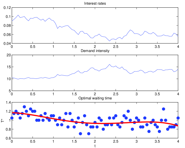
This figure shows that as interest rates decrease, the demand intensity and the OWT increase. With the increase in the demand intensity and the decrease in the interest rates level, OWT decreases since, in these circumstances, the seller gets more offers and his payoff is discounted by a lower factor. This figure also demonstrates that changing market conditions have a broad impact on the house sale process. In a low-interest rate and high-demand environment, the seller keeps the house on the market for a shorter time than he would in a high-interest and low-demand environment.

Figure 9: Single price evolution of a real asset in a realization of interest rates and a stochastic demand function

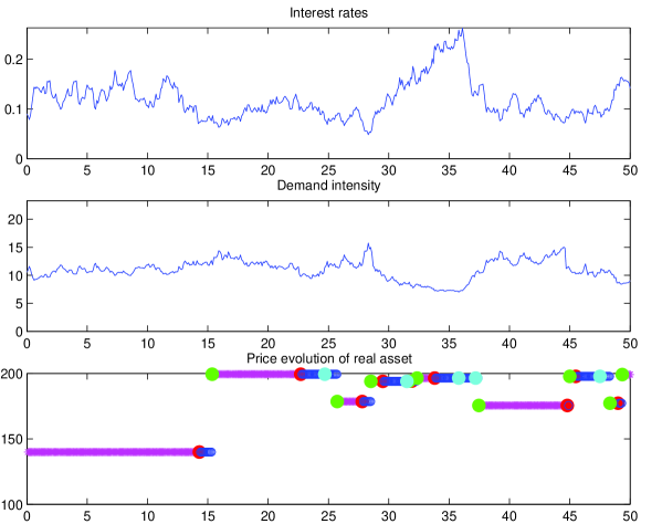
Figure 9 illustrates the house sale price along with the corresponding functions of interest rates and demand intensities over a fifty-year period. The price evolution in the third row shows the random occupation periods, times of exogenous shocks due to personal crises or profit opportunities. It also includes whether or not the price process results in success with the appropriate labels shown in the legend of Figure 10. This figure extends the price evolution shown in Figure 9.

Figure 10 studies the decision process of the seller. The occupation period, decision of sale, time on the market, and time of the sale are illustrated in the figure. Until the moment of sale, all of these time periods are shown at the same price level which constitutes the price that the seller paid at his initial purchase of the house.

In Figure 10, pink circles represent the occupation period in which the seller decides not to sell the asset. Pink circles are always followed by a black or red dot which represents the decision of sale due to a either a profit opportunity or a personal crisis, respectively. At the time of sale decision, the seller sets an OWT, taking the current market conditions into account. The waiting period is shown by the blue circles. After this waiting time, a green or magenta dot follows, signifying the event of sale and no-sale respectively. If there is a sale, a new period starts with the occupation period of the new owner of the house.

Figure 10: Single price evolution of a real asset with illustration of subperiods and sale or no sale outcomes

Figure 11: Expected price evolution of a real asset in a single realization of interest rates and a stochastic demand function

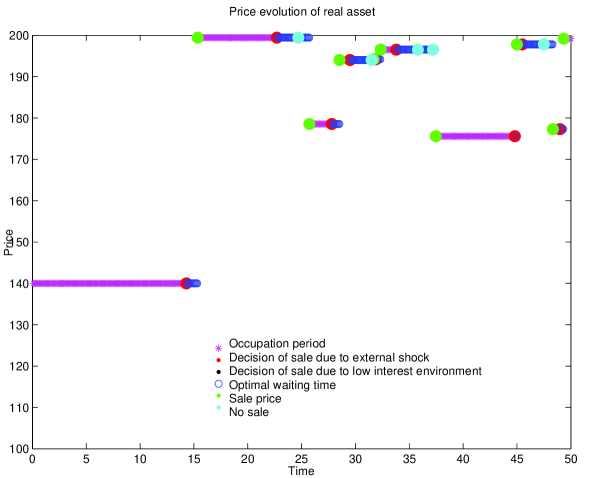
If the seller does not sell the house, he lowers the reservation and list prices and sets a new OWT by using the new parameters and current market conditions. Blue circles follow the magenta dot in the case of no-sale. In this second sale attempt, he may still sell the asset for a price higher than his initial reservation price, but this probability is less than in the first attempt. Our results illustrate this conclusion, as in the figure, four cases result in no-sales, only one of which is sold for a price higher than the initial reservation price. The seller may not sell the house in this attempt either. In this case, he will be further lower his reservation and list prices. However, this probability is also lower: out of four cases of no-sale, only one seller encountered two successive failed attempts.

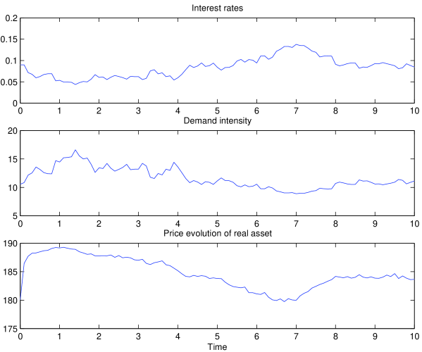
Figure 11 graphs the expected price evolution of the real asset without considering occupation periods or exogenous shocks. This figure shows the mean sale price if the seller posts the house for sale at a given time. This figure still assumes that the seller sets an optimal waiting time and has his own reservation price. This figure supports the conclusions from the single simulation. Note that the expected sale price declines (increases) with a decrease (increase) in the demand and a rise (fall) in interest rates.

Our simulation results show that the fluctuation in house prices are driven by interest rates, demand, and time-on-the-market (TOM). In Figure 9, interest rates increase between the 25th and 40th year, and this increase results in two unsuccessful sale attempts in Figure 10. During this period, the reservation price of the house is close to its maximum and, with the high-interest and low-demand environment, the seller could not succeed in selling the house in two trials. Eventually, the seller sells the asset in the third trial with a significant discount compared to his reservation price.

4.3 The Subprime Lending Crisis

Our simulation provides some insights into the housing market crash observed during the subprime lending crisis (for a review see Crouhy, Jarrow, Turnbull [8]). The record low borrowing rates during 1999-2004 increased housing affordability with the corresponding up-trend in home prices as shown in Figure 1. When borrowing rates increased and home buyers’ mortgage contracts began to reset to these higher rates, low credit borrowers had a difficult time making their monthly payments. They either defaulted or were forced to put their homes up for sale. This coincides exactly with our modeling of a personal crisis. Due to this shock, the home owner had to sell his house in an unfavorable market: high interest rates and low demand. As shown in our simulation results, the expected price in such a market environment is low.

Another catalyst for subprime defaults were the higher reservation prices locked in during the bull period. Although demand should have been low during this period, borrowers still obtained financing - helped by the lower standards of the mortgage originators. To support this view, note that during 2002-2006, the Combined Loan to Value (CLTV) ratio increased. In the subprime category, it rose to 88% from 81% and in Alt-A category, it rose to 85% from 73%. When the subprime homes were put on the market, they could not get any offers matching their list price. As we discussed in our simulation, in a high-interest and low demand environment, it is very difficult to sell a property with a high reservation price. Since most of the subprime borrowers paid for their homes at record high values, they had to lower their reservation prices during the sale process. This result is similar to our successive no-sale events when the reservation price of the owner is close to $p_{\max}$.

5 Conclusion

This paper proposes a new model to describe the evolution of housing prices. We include exogenous shocks to the real estate market that may be the result of a profit opportunity or personal crisis. We investigate the sale process by introducing a new model for analyzing the time-on-the-market (TOM) with a new construct, the optimal waiting time (OWT). We study the comparative statistics of the OWT with respect to the model’s parameters such as the arrival intensity, the offer withdrawal (cancelation) rates, and interest rates. We specifically look at the pairwise impact of these parameters and how they affect the resulting OWT in the different regions of the surface. We incorporate our theory of the OWT into a price evolution analysis that also includes an occupation period, a personal crisis or profit-taking opportunity, and the deterministic updating of model parameters with the occurrence of the sale. Our model specifically considers the occurrence of sale, no sale conditions, and how the seller responds to the no sale scenario. Our simulation results show that it becomes more difficult to sell a house in a high-interest, low-demand environment and that these conditions may require the seller to sell the asset below his initial reservation price. This results in a dynamic, time-dependent, and stochastic house price process which provides some insights into the recent subprime credit crisis.

Appendix A Appendix: Auxiliary Model

We will derive the auxiliary model in this appendix. Buyers make offers with $\exp(\lambda)$ and their offers are distributed uniformly with $U(p_{\min},p_{\max})$. The seller’s reservation price is $p_{\min}$. After making an offer, a buyer may withdraw his offer with distribution $\exp(\mu)$. Interest rate is constant and equals $r$. The seller wants to maximize expected payoff with respect to waiting time, $T$. Let $N(T)$ be the number of offers received by time $T$ and $\xi_{i}$ be the offer from buyer $i$, $B_{i}$, at the arrival time, $A_{i}$, and $\xi_{(i)}$ be the $i$th minimum offer received by the seller. With these assumptions, the discounted expected payoff, $u(.)$, is a function of $T$, $\lambda$, $\mu$, $p_{\min}$, $p_{\max}$, and $r$.

$$u(.) = \mathbb{E}\left[\mathbb{E}\left[X|N(T)=n\right]\right]$$

$$= \sum_{n=0}^{\infty}\mathbb{E}\Big{[}\xi_{(n)}e^{-rT}1\!\!1_{[B_{n}\text{ is still interested}]}+\xi_{(n-1)}e^{-rT}1\!\!1_{[B_{n-1}\text{ is still interested and }\xi_{(n)}\text{ is withdrawn}]}$$

$$\text{ \ \ \ \ }\ldots+\xi_{(1)}e^{-rT}1\!\!1_{[B_{1}\text{ is still interested and }\xi_{(n)}...\xi_{(2)}\text{ are withdrawn}]}|N(T)=n\Big{]}\mathbb{P}\left(N(T)=n\right)$$

$$= \sum_{n=0}^{\infty}\sum_{i=1}^{n}\mathbb{E}\left[\xi_{(n-i+1)}e^{-rT}1\!\!1_{[B_{n-i+1}\text{ is still interested and }\xi_{(n)}...\xi_{(n-i+2)}\text{ are withdrawn}]}|N(T)=n\right]\times$$

$$\text{ \ \ \ \ \ }\mathbb{P}\left(N(T)=n\right)$$

$$= \sum_{n=0}^{\infty}\sum_{i=1}^{n}\mathbb{E}\left[\xi_{(n-i+1)}|N(T)=n\right]\times\mathbb{E}\left[e^{-rT}1\!\!1_{[B_{n-i+1}\text{ is still interested}]}|N(T)=n\right]\times$$

$$\text{ \ \ \ \ \ }\mathbb{E}\left[1\!\!1_{[\xi_{(n)}...\xi_{(n-i+2)}\text{ are withdrawn}]}|N(T)=n\right]\mathbb{P}\left(N(T)=n\right).$$

Each of the components of the sum is as follows

$$\mathbb{E}\left[\xi_{(i)}|N(T)=n\right] = p_{\min}+\frac{(p_{\max}-p_{\min})i}{n+1},$$

$$\mathbb{E}\left[1\!\!1_{[B_{i}\text{ is still interested}]}|N(T)=n\right] = \int_{0}^{T}\frac{1}{T}e^{-\mu x}dx=\frac{1}{\mu T}(1-e^{-\mu T}):=1-f(T),$$

$$\mathbb{E}\left[1\!\!1_{[\xi_{(n)}...\xi_{(n-i+2)}\text{ are withdrawn}]}|N(T)=n\right] = [f(T)]^{i-1},$$

$$\mathbb{P}\left(N(T)=n\right) = \frac{(\lambda T)^{n}e^{-\lambda T}}{n!}.$$

Using these components, expected payoff becomes

$$u(.) = \sum_{n=0}^{\infty}\sum_{i=1}^{n}\left(p_{\min}+\frac{(p_{\max}-p_{\min})(n-i+1)}{n+1}\right)e^{-rT}(1-f(T))(f(T))^{i-1}\left(\frac{(\lambda T)^{n}e^{-\lambda T}}{n!}\right)$$

$$= g(T)\sum_{n=0}^{\infty}\frac{(\lambda T)^{n}}{n!}\sum_{i=1}^{n}\left(p_{\max}(f(T))^{i-1}-\frac{(p_{\max}-p_{\min})}{n+1}i(f(T))^{i-1}\right),$$

where $g(T)=(1-f(T))e^{-rT}e^{-\lambda T}.$ We use the following facts in the final computation.

$$\sum_{i=1}^{n}ix^{i-1} = \frac{d(\sum_{i=1}^{n}x^{i})}{dx}=\frac{d(\frac{1-x^{n+1}}{1-x})}{dx}=\frac{nx^{n+1}-(n+1)x^{n}+1}{(1-x)^{2}}$$

and

$$\sum_{i=1}^{n}x^{i-1} = \frac{1-x^{n}}{1-x}.$$

Finally, the discounted expected payoff equals

$$u(T,\lambda,\mu,p_{\min},p_{\max},r) = g(T)\sum_{n=0}^{\infty}\frac{(\lambda T)^{n}}{n!}\Big{[}\frac{p_{\max}-p_{\min}}{(n+1)(1-f(T))^{2}}\left(nf(T)^{n+1}-(n+1)f(T)^{n}+1\right)$$

$$\text{ \ \ \ \ \ \ \ \ \ }+p_{\max}\frac{1-f(T)^{n}}{1-f(T)}\Big{]}$$

$$= \frac{-g(T)(p_{\max}-p_{\min})}{(1-f(T))^{2}}(f(T)e^{\lambda Tf(T)}-\frac{1}{\lambda T}(e^{\lambda Tf(T)}-1)-e^{\lambda Tf(T)}$$

$$\text{ \ \ \ \ \ \ \ \ \ }+\frac{1}{\lambda T}(e^{\lambda T}-1))+\frac{p_{\max}g(T)(e^{\lambda T}-e^{\lambda Tf(T)})}{1-f(T)},$$

where $f(T)=1-\frac{1}{\mu T}(1-e^{-\mu T})$ and $g(T)=(1-f(T))e^{-rT}e^{-\lambda T}$.

Appendix B Appendix: Theorem 3.1

We first establish some auxiliary results that will be used while proving Theorem 3.1. Lemma B.1 gives us the formula for the conditional probability, which is conditioned on $\mathcal{F}_{t}$ and $N(t)=n$, that an offer value is smaller than the announced list price at its arrival time.

Lemma B.1

Let $\varphi(t)=\mathbb{P}\{\xi_{1}<L(A_{1})|\mathcal{F}_{t},N(t)=n\}$ for $n\geq 1$. Then,

$$\varphi(t)=\frac{1}{\Lambda(t)}\int_{0}^{t}\lambda(a)F_{\xi}\big{(}L(a)\big{)}\mathrm{d}a.$$

Proof.    Given $A_{1}=a$, the event $\{\xi_{1}<L(A_{1})\}$ is independent of $\mathcal{F}_{t}$ and $N(t)$. Thus,

$$\varphi(t) = \int_{0}^{t}f_{A|\{\mathcal{F}_{t},N(t)=n\}}(a)\mathbb{P}\{\xi_{1}<L(a)\}\mathrm{d}a$$

$$= \frac{1}{\Lambda(t)}\int_{0}^{t}\lambda(a)F_{\xi}\big{(}L(a)\big{)}\mathrm{d}a.$$

$\blacksquare$

The following lemma provides the formula for the conditional probability, which is conditioned on $\mathcal{F}_{t}$ and $N(t)=n$, that none of the offers arrived in the time interval $[0,t]$ is greater than the announced sale at their arrival times.

Lemma B.2

$\mathbb{P}\{\beta>t|\mathcal{F}_{t},N(t)=n\}=\varphi(t)^{n}$ for $n\geq 1$.

Proof.

$$\mathbb{P}\{\beta>t|\mathcal{F}_{t},N(t)=n\} = \mathbb{P}\Big{(}\bigcap_{i=0}^{n}\{\xi_{i}<L(A_{i})\}|\mathcal{F}_{t},N(t)=n\Big{)}$$

$$= \mathbb{P}\{\xi_{1}<L(A_{1})|\mathcal{F}_{t},N(t)=n\}^{n}=\varphi(t)^{n}.$$

$\blacksquare$

Now, we calculate the conditional density of $\beta$, $f_{\beta|\{\mathcal{F}_{t},N(t)=n,\beta\leq t\}}(s)$, conditioned on $\mathcal{F}_{t}$, $N(t)=n$, and $\beta\leq t$.

Lemma B.3

$f_{\beta|\{\mathcal{F}_{t},N(t)=n,\beta\leq t\}}(s)=\frac{\lambda(s)}{\Lambda(t)}$.

Proof.    Let $i(\beta)$ be the index of the offer at time $\beta$. Then,

$$\mathbb{P}\{\beta\leq s|\mathcal{F}_{t},N(t)=n,\beta\leq t\}=\mathbb{P}\{A_{i(\beta)}\leq s|\mathcal{F}_{t},N(t)=n,\beta\leq t\}.$$

Since $\beta\leq t$, we know that $i(\beta)\leq n$. Given $N(t)=n$ and $\mathcal{F}_{t}$, all offer arrival times are independently distributed over $[0,t]$ according to density $\frac{\lambda(s)}{\Lambda(t)}$. Thus,

$$\mathbb{P}\{\beta\leq s|\mathcal{F}_{t},N(t)=n,\beta\leq t\}=\frac{\Lambda(s)}{\Lambda(t)}.$$

Thus, $f_{\beta|\{\mathcal{F}_{t},N(t)=n,\beta\leq t\}}(s)=\frac{\lambda(s)}{\Lambda(t)}$. $\blacksquare$

In Lemma B.4, we derive the conditional probability, conditioned on $\mathcal{F}_{t}$ and $N(t)=n$, of an offer, which is not withdrawn up to time $t$ and greater than the reservation price but not exceeding the list price at its arrival time, to be greater than a positive real number $y$.

Lemma B.4

Let $\psi(t,y)=\mathbb{P}\{\xi_{1}1\!\!1_{\{R\leq\xi_{1}<L(A_{1})\}}1\!\!1_{\{\tau_{1}\geq t-A_{1}\}}>y|\mathcal{F}_{t},N(t)=n\}$ for $n\geq 1$. Then,

$$\psi(t,y)=\frac{1}{\Lambda(t)}\int_{0}^{t}\lambda(a)\Big{(}1-F_{\tau}(t-a)\Big{)}\Big{(}F_{\xi}\big{(}L(a)\vee y\big{)}-F_{\xi}\big{(}R\vee y\big{)}\Big{)}\mathrm{d}a.$$ (2.17)

Proof.    Conditioned on $A_{1}=a$, events $\{\tau_{1}\geq t-A_{1}\}$ and $\{R\leq\xi_{1}<L(A_{1})\}$ are independent of each other as well as being independent of $\mathcal{F}_{t}$ and $N(t)$. Thus,

$$\psi(t,y) = \frac{1}{\Lambda(t)}\int_{0}^{a}\lambda(a)\mathbb{P}\{\tau_{1}\geq t-a\}\mathbb{P}\{\xi_{1}1\!\!1_{\{R\leq\xi_{1}<L(a)\}}>y\}$$

$$= \frac{1}{\Lambda(t)}\int_{0}^{t}\lambda(a)\Big{(}1-F_{\tau}(t-a)\Big{)}\Big{(}F_{\xi}\big{(}L(a)\vee y\big{)}-F_{\xi}\big{(}R\vee y\big{)}\Big{)}\mathrm{d}a.$$

$\blacksquare$

Let $p_{n}(t)=\mathbb{P}\{N(t)=n|\mathcal{F}_{t}\}$. The following summation formula will also be used in the proof of Theorem 3.1, and gives us the conditional moment generating function of a Poisson process with stochastic intensity.

Lemma B.5

For $q>0$, the following holds.

$$\sum_{n=0}^{\infty}p_{n}(t)q^{n} = \exp\big{(}\Lambda(t)(q-1)\big{)}.$$

We now start proving Theorem 3.1. Let $X_{1}(t)$ be the first term in (3.9), and $X_{2}(t)$ be the second term in (3.9). Let us define $P_{1}(t|\mathcal{F}_{t})=\mathbb{E}[X_{1}(t)|\mathcal{F}_{t}]$, and $P_{2}(t|\mathcal{F}_{t})=\mathbb{E}[X_{2}(t)|\mathcal{F}_{t}]$. We first calculate $P_{1}(t|\mathcal{F}_{t})$.

$$P_{1}(t|\mathcal{F}_{t})=\sum_{n=0}^{\infty}p_{n}(t)\mathbb{E}\big{[}X_{1}(t)|\mathcal{F}_{t},N(t)=n\big{]}.$$

Put $M(t)=\max_{0\leq i\leq N(t)}\xi_{i}1\!\!1_{\{\xi_{i}\geq R\}}1\!\!1_{\{\tau_{i}\geq t-A_{i}\}}$. Then,

$$\mathbb{E}[X_{1}(t)|\mathcal{F}_{t},N(t)=n]=\mathrm{e}^{-\int_{0}^{t}r(s)\mathrm{d}s}\mathbb{E}\big{[}M(t)1\!\!1_{\{\beta>t\}}|\mathcal{F}_{t},N(t)=n\big{]}.$$ (2.18)

The expectation in (2.18) can be calculated by conditioning on the event $\{\beta>t\}$.

$$\mathbb{E}\big{[}M(t)1\!\!1_{\{\beta>t\}}|\mathcal{F}_{t},N(t)=n\big{]} = \mathbb{P}\{\beta>t|\mathcal{F}_{t},N(t)=n\}\mathbb{E}\big{[}M(t)|\mathcal{F}_{t},N(t)=n,\beta>t\big{]}$$

$$= \varphi(t)^{n}\mathbb{E}\big{[}M(t)|\mathcal{F}_{t},N(t)=n,\beta>t\big{]}.$$

Since $M(t)$ is positive, its conditional expectation can be calculated by integrating $\mathbb{P}\{M(t)>y|\mathcal{F}_{t},N(t)=n,\beta>t\}$ with respect to $y$ over $[0,\infty]$. Let us calculate $\mathbb{P}\{M(t)>y|\mathcal{F}_{t},N(t)=n,\beta>t\}$.

$$\mathbb{P}\{M(t)>y|\mathcal{F}_{t},N(t)=n,\beta>t\}$$

$$=1-\Big{(}1-\mathbb{P}\big{\{}\xi_{1}1\!\!1_{\{\xi_{1}\geq R\}}1\!\!1_{\{\tau_{1}\geq t-A_{1}\}}>y|\mathcal{F}_{t},N(t)=n,\xi_{1}<L(A_{1})\big{\}}\Big{)}^{n}$$

$$=1-\Big{(}1-\frac{\mathbb{P}\{\xi_{1}1\!\!1_{\{R\leq\xi_{1}\leq L(A_{1})\}}1\!\!1_{\{\tau_{1}\geq t-A_{1}\}}>y|\mathcal{F}_{t},N(t)=n\}}{\mathbb{P}\{\xi_{1}<L(A_{1})|\mathcal{F}_{t},N(t)=n\}}\Big{)}^{n}$$

$$=1-\Big{(}1-\frac{\psi(t,y)}{\varphi(t)}\Big{)}^{n}$$

Integrating $\mathbb{P}\{M(t)>y|\mathcal{F}_{t},N(t)=n,\beta>t\}$ over $y$, we obtain $\mathbb{E}[M(t)|\mathcal{F}_{t},N(t)=n,\beta>t]$.

$$\mathbb{E}[M(t)|\mathcal{F}_{t},N(t)=n,\beta>t] = \int_{0}^{\infty}\mathbb{P}\{M(t)>y|\mathcal{F}_{t},N(t)=n,\beta>t\}\mathrm{d}y$$ (2.19)

$$= \int_{0}^{\infty}\Big{(}1-\big{(}1-\frac{\psi(t,y)}{\varphi(t)}\big{)}^{n}\Big{)}\mathrm{d}y.$$

Noting that $\psi(t,y)=0$ a.s. when $y>L_{0}$, we can further simplify (2.19) to

$$\mathbb{E}[M(t)|\mathcal{F}_{t},N(t)=n,\beta>t]=L_{0}-\int_{0}^{L_{0}}\big{(}1-\frac{\psi(t,y)}{\varphi(t)}\big{)}^{n}\mathrm{d}y.$$

As a result, $\mathbb{E}[X_{1}(t)|\mathcal{F}_{t},N(t)=n]$ is equal to

$$\mathbb{E}[X_{1}(t)|\mathcal{F}_{t},N(t)=n]=\mathrm{e}^{-\int_{0}^{t}r(s)\mathrm{d}s}\big{(}L_{0}\varphi(t)^{n}-\int_{0}^{L_{0}}\big{(}\varphi(t)-\psi(t,y)\big{)}^{n}\mathrm{d}y\big{)}.$$

Now, we average $\mathbb{E}[X_{1}(t)|\mathcal{F}_{t},N(t)=n]$ over $N(t)$. By using Fubini’s theorem and Lemma B.5, we obtain

$$P_{1}(t|\mathcal{F}_{t})=\mathrm{e}^{-\int_{0}^{t}r(s)\mathrm{d}s}\mathrm{e}^{\Lambda(t)(\varphi(t)-1)}\Big{(}L_{0}-\int_{0}^{L_{0}}\mathrm{e}^{-\Lambda(t)\psi(t,y)}\mathrm{d}y\Big{)}.$$

Let us now calculate $P_{2}(t|\mathcal{F}_{t})$. It is equal to

$$P_{2}(t|\mathcal{F}_{t})=\sum_{n=0}^{\infty}p_{n}(t)\mathbb{E}[X_{2}(t)|\mathcal{F}_{t},N(t)=n].$$

where $\mathbb{E}[X_{2}(t)|\mathcal{F}_{t},N(t)=n]$ is calculated as

$$\mathbb{E}[X_{2}(t)|\mathcal{F}_{t},N(t)=n] = \mathbb{E}\big{[}\mathrm{e}^{-\int_{0}^{\beta}r(s)\mathrm{d}s}\xi_{i(\beta)}1\!\!1_{\{\beta\leq t\}}|\mathcal{F}_{t},N(t)=n\big{]}$$

$$= \mathbb{P}\{\beta\leq t|\mathcal{F}_{t},N(t)=n\}\mathbb{E}\big{[}\mathrm{e}^{-\int_{0}^{\beta}r(s)\mathrm{d}s}\xi_{i(\beta)}|\mathcal{F}_{t},N(t)=n,\beta\leq t\big{]}$$

$$= \big{(}1-\varphi(t)^{n}\big{)}\int_{0}^{t}f_{\beta|\{\mathcal{F}_{t},N(t)=n,\beta\leq t\}}(a)\mathrm{e}^{-\int_{0}^{a}r(s)\mathrm{d}s}\mathbb{E}\big{[}\xi_{i(a)}\big{]}.$$

The last equality follows from the fact that the magnitude of $\xi_{i(\beta)}$ is independent of $\mathcal{F}_{t}$ and $N(t)$, and only depends on $a$ given the event $\{\beta=a\}$. Note also that

$$\mathbb{E}[\xi_{i(a)}] = \mathbb{E}[\xi_{1}|\xi_{1}\geq L(a)]$$

$$= \frac{\int_{L(a)}^{\infty}xf_{\xi}(x)\mathrm{d}x}{1-F_{\xi}\big{(}L(a)\big{)}}$$

Thus,

$$\mathbb{E}[X_{2}(t)|\mathcal{F}_{t},N(t)=n] = \big{(}1-\varphi(t)^{n}\big{)}\int_{0}^{t}\int_{L(a)}^{\infty}f_{\beta|\{\mathcal{F}_{t},N(t)=n,\beta\leq t\}}(a)\frac{\exp(-\int_{0}^{a}r(s)\mathrm{d}s)}{1-F_{\xi}\big{(}L(a)\big{)}}xf_{\xi}(x)\mathrm{d}x\mathrm{d}a$$

$$= \big{(}1-\varphi(t)^{n}\big{)}\int_{0}^{t}\int_{L(a)}^{\infty}\frac{\lambda(a)\exp\big{(}-\int_{0}^{a}r(s)\mathrm{d}s\big{)}}{\Lambda(t)\big{(}1-F_{\xi}\big{(}L(a)\big{)}\big{)}}f_{\xi}(x)x\mathrm{d}x\mathrm{d}a.$$

$P_{2}(t|\mathcal{F}_{t})$ is obtained by averaging $\mathbb{E}[X_{2}(t)|\mathcal{F}_{t},N(t)=n]$ over $N(t)$. By using Lemma B.5, we obtain

$$P_{2}(t|\mathcal{F}_{t})=\big{(}1-\mathrm{e}^{\Lambda(t)(\varphi(t)-1)}\big{)}\int_{0}^{t}\int_{L(a)}^{\infty}\frac{\lambda(a)\exp\big{(}-\int_{0}^{a}r(s)\mathrm{d}s\big{)}}{\Lambda(t)\big{(}1-F_{\xi}\big{(}L(a)\big{)}\big{)}}f_{\xi}(x)x\mathrm{d}x\mathrm{d}a.$$

This completes the proof since $P(t|\mathcal{F}_{t})=P_{1}(t|\mathcal{F}_{t})+P_{2}(t|\mathcal{F}_{t})$.

Appendix C Appendix: Parameter Assumptions

Parameter	Value
Arrival intensity ($\lambda$)	5
Withdrawal intensity ($\mu$)	5
Interest rate ($r$)	0.1
Reservation price ($R$)	140
List price ($L$)	180
Waiting averseness ($\gamma$)	0.1
$p_{\min}$	100
$p_{\max}$	200

Table 1: Default parameter values in OWT analysis in Section 2

Parameter	Value
Withdrawal intensity ($\mu$)	10
Occupation period ($O$)	$U(4,6)$
Rate of personal crisis	$Exp(10)$
Initial reservation price($R_{0}$)	140
Initial list price ($L_{0}$)	200
Waiting averseness ($\gamma$)	0.8
Interest rate threshold ($\phi$)	0.06
$p_{\min}$	100
$p_{\max}$	200
$K_{1}$	0.5
$K_{2}$	1000
$\theta$	0.1
$\sigma$	0.08
$\kappa$	0.25
$r_{0}$	0.09

Table 2: Default parameter values in the simulation

References

- [1] Bailey, M., Muth, R. and Nourse, H. (1963), “A Regression Method for Real Estate Price Index Construction”, Journal of the American Statistical Association, 58: 933-942
- [2] Capozza, D.R., Hendershott, P.H. and Mack, C. (2004), “An Anatomy of Price Dynamics in Illiquid Markets: Analysis and Evidence from Local Housing Markets ”, Real Estate Economics, 32(1), 1-32.
- [3] Case, K.E. and Shiller, R. (1987), “Prices of Single-Family Homes Since 1970: New Indexes For Four Cities”, New England Economic Review, Sept/Oct: 45-56.
- [4] Case, K.E. and Shiller, R. (1990), “Forecasting Prices and Excess Returns in the Housing Market”, Journal of the American Real Estate and Urban Economics Association, 18(3), 263-273.
- [5] Case, B. and Quigley, J.M. (1991), “The Dynamics of Real Estate Prices”, The Review of Economics and Statistics, 73(1), 50-58.
- [6] Cubbin, J. (1974), “Price, Quality, and Selling Time in the Housing Market”, Applied Economics, 6, 171-187.
- [7] Cox, J.C., Ingersoll, J.E. and Ross, S.A. (1985), “A Theory of the Term Structure of Interest Rates”, Econometrica, 53: 385-407.
- [8] Crouhy, M., Jarrow, R. and Turnbull, S. (2008) “The Subprime Credit Crisis of 07,” Journal of Derivatives, 16 (4), (Fall 2008), 81 - 110.
- [9] Evans, J., Henderson, V. and Hobson, D. (2007), “Optimal Timing For an Indivisible Asset Sale ”, to appear in Mathematical Finance.
- [10] Forgey, F.A., Rutherford, R.C. and Springer, T.A. (1996), “Search and Liquidity in Single-Family Housing”, Real Estate Economics, 24(3), 273-292.
- [11] Genesove, D. and Mayer, C. (1998), “Equity and Time to Sale in the Real Estate Market”, The American Economic Review, 87(3), 255-269.
- [12] Goetzmann, W. and Peng, L. (2006), “Estimating House Price Indexes in the Presence of Seller Reservation Prices”, The Review of Economics and Statistics, 88(1): 100–112.
- [13] Glower, M., Haurin, D.R., Hendershott, P.H. (1998), “Selling Time and Selling Price: The Influence of Seller Motivation”, Real Estate Economics, 26(4), 719-740.
- [14] Grenadier, S.R. and Wang, N. (2005), “Investment timing, agency, and information”, Journal of Financial Economics, 75(3), 493-533.
- [15] Haurin, D.R. (1988), “The Duration of Marketing Time of Residential Housing”, Journal of the American Real Estate and Urban Economics Association, 16(4), 396-410.
- [16] Kalra, R., Chan, C.C. and Lai, P. (1997), “Time on Market and Sales Price of Residential Housing: A Note”, Journal of Economics and Finance, 21(2), 63-66.
- [17] Knight, J.R. (2002), “Listing Price, Time on Market, and Ultimate Selling Price: Causes and Effects of Listing Price Changes”, Real Estate Economics, 30(2), 213-237.
- [18] Krainer, J. and LeRoy, S.F. (2002), “Equilibrium valuation of illiquid assets”, Economic Theory, 19, 223-242.
- [19] Lin, Z. and Vandell, K.D. (2007) “Illiquidity and Pricing Biases in the Real Estate Market”, Real Estate Economics, 35(3), 291-330.
- [20] Lucas, R.E. and Prescott, E.C. (1974), “Equilibrium Search and Unemployment”, Journal of Economic Theory, 7, 188-209.
- [21] McMillen, D.P. and Thorsnes, P. (2006) “Housing Renovations and the Quantile Repeat-Sales Price Index”, Real Estate Economics, 34(4), 567-584.
- [22] Miller, N.G. (1978), “Time on the Market and Selling Price”, Journal of the American Real Estate and Urban Economics Association, 6(2), 164-174.
- [23] Ortalo-Magné, F. and Rady S. (2006), “Housing Market Dynamics: On the Contribution of Income Shocks and Credit Constraints”, Review of Economic Studies, 73, 459-485.
- [24] Poterba, J.M. (1991), “House Price Dynamics: The Role of Tax Policy and Demography”, Brookings Papers on Economic Activity, 143-203.
- [25] Resnick, I.S. (1992), “Adventures in Stochastic Processes”, Birkhauser Boston.
- [26] Sarr, T. (1988), “A Note on Optimal Price Cutting Behavior under Demand Uncertainty”, The Review of Economics and Statistics, 70(2), 336-339.
- [27] Stein, J.C. (1995), “Prices and Trading Volume in the Housing Market: A Model with Down-Payment Effects”, Quarterly Journal of Economics, 110(2), 379-406.
- [28] Taylor, C. R. (1999), “Time-on-the-Market as a Sign of Quality”, Review of Economic Studies, 66, 555-578.
- [29] Wheaton, W.C. (1990), “Vacany, search, and prices in a housing market matching model”, Journal of Political Economy, 61, 1270-1292.
- [30] Williams, J.T. (1995), “Pricing real assets with costly search”, Review of Financial Studies, 8, 55-90.
- [31] Yavas, A. (1992), “A Simple Search and Barganing Model of Real Estate Markets”, Journal of the American Real Estate and Urban Economics Association, 20(4), 533-548.