An analytic approach to number counts of weak-lensing peak detections

We develop and apply an analytic method to predict peak counts in weak-lensing surveys. It is based on the theory of Gaussian random fields and suitable to quantify the level of spurious detections caused by chance projections of large-scale structures as well as the shape and shot noise contributed by the background galaxies. We compare our method to peak counts obtained from numerical ray-tracing simulations and find good agreement at the expected level. The number of peak detections depends substantially on the shape and size of the filter applied to the gravitational shear field. Our main results are that weak-lensing peak counts are dominated by spurious detections up to signal-to-noise ratios of 3–5 and that most filters yield only a few detections per square degree above this level, while a filter optimised for suppressing large-scale structure noise returns up to an order of magnitude more.

1 Introduction

Wide-area surveys for weak gravitational lensing can be and have been used for counting peaks in the shear signal, which are commonly interpreted as the signature of sufficiently massive dark-matter halos. However, such detections are clearly contaminated by spurious detections caused by the chance superposition of large-scale structures, and even by the shape- and shot-noise contributions from the background galaxies used to sample the foreground shear field. As a function of the peak height, what is the contribution of genuine halos to these detections, and how much do the large-scale structure and the other sources of noise contribute?

Given the power of lensing-peak number counts as a cosmological probe (Marian et al., 2009; Kratochvil et al., 2009; Dietrich & Hartlap, 2009), we address this question here after developing a suitable analytic approach based on peak counts in Gaussian random fields, as laid out by Bardeen et al. (1986). It is reasonable to do so even though at least the high peaks are caused by halos in the non-Gaussian tail of the density fluctuations because the noise and large-scale structures contributions remain Gaussian, and thus at least the contamination of the counts can be well described analytically. Peaks with the highest signal-to-noise ratios are expected to be more abundant than predicted based on Gaussian random fields.

Weak-lensing data are filtered to derive peak counts from them. Several linear filters have been proposed and used in the literature. They can all be seen as convolutions of the measured shear field with filter functions of different shapes. Many shapes have been proposed for different purposes (Schneider et al., 1998; Schirmer et al., 2004; Maturi et al., 2005). One filter function, called the optimal filter later on, was designed specifically to suppress the contribution from the large-scale structure by maximising the signal-to-noise ratio of halo detections against the shear field of the large-scale structure.

We study three such filters here, with the optimal filter among them. Results will differ substantially, arguing for a careful filter choice if halo detections are the main goal of the application. We compare our analytic results to a numerical simulation and show that both agree at the expected level. We begin in § 2 with a brief summary of gravitational lensing as needed here and describe filtering methods in § 3. We present our analytic method in § 4 and compare it to numerical simulations in § 5, where we also show our main results. Conclusions are summarised in § 6. In Appendix A, we show predictions of peak counts and the noise levels in them for several planned and ongoing weak-lensing surveys.

2 Gravitational lensing

Isolated lenses are characterised by their lensing potential

$$\psi(\@vec{\theta})\equiv\frac{2}{c^{2}}\frac{D_{\rm ds}}{D_{\rm d}D_{\rm s}}\int\Phi(D_{\rm d}\@vec{\theta},z)\,\mathrm{d}z\;,$$ (1)

where $\Phi$ is the Newtonian gravitational potential and $D_{\rm s,d,ds}$ are the angular-diameter distances between the observer and the source, the observer and the lens, and the lens and the source, respectively. The potential $\psi$ relates the angular positions $\@vec{\beta}$ of the source and $\@vec{\theta}$ of its image on the observer’s sky through the lens equation

$$\@vec{\beta}=\@vec{\theta}-\@vec{\nabla}\psi\;.$$ (2)

Since sources such as distant background galaxies are much smaller than the typical scale on which the lens properties change and the angles involved are small, it is possible to linearise Eq. (2) such that the induced image distortion is expressed by the Jacobian

$$A=(1-\kappa)\left(\begin{array}[]{cc}1-g_{1}&g_{2}\\ g_{2}&1+g_{1}\\ \end{array}\right)\,,$$ (3)

where $\kappa=\nabla^{2}\psi/2$ is the convergence responsible for the isotropic magnification of an image relative to its source, and $g(\@vec{\theta})=\gamma(\@vec{\theta})/[1-\kappa(\@vec{\theta})]$ is the reduced shear quantifying its distortion. Here, $\gamma_{1}=\left(\psi_{,11}-\psi_{,22}\right)/2$ and $\gamma_{2}=\psi_{,12}$ are the two components of the complex shear. Since the angular size of the source is unknown, only the reduced shear can be estimated starting from the observed ellipticity of the background sources,

$$\epsilon=\frac{\epsilon_{\rm s}+g}{1+g^{*}\epsilon_{\rm s}}\;,$$ (4)

where $\epsilon_{\mathrm{s}}$ is the intrinsic ellipticity of the source and the asterisk denotes complex conjugation.

3 Measuring weak gravitational lensing

3.1 Weak lensing estimator

In absence of intrinsic alignments between background galaxies due to possible tidal interactions (Heavens & Peacock, 1988; Schneider & Bridle, 2009), the intrinsic source ellipticities in Eq. (4) average to zero in a sufficiently large source sample. An appropriate and convenient measure for the lensing signal is the weighted average over the tangential component of the shear $\gamma_{\rm t}$ relative to the position $\@vec{\theta}$ on the sky,

$$\tilde{A}(\@vec{\theta})=\int\mathrm{d}^{2}\theta^{\prime}\gamma_{\rm t}(\@vec{\theta^{\prime}},\@vec{\theta})Q(|\@vec{\theta^{\prime}}-\@vec{\theta}|)\;.$$ (5)

The filter function $Q$ determines the statistical properties of the estimator $\tilde{A}$. We shall consider three filter functions here which will be described in § 3.2.

Data on gravitational lensing by a mass concentration can be modeled by a signal $s(\@vec{\theta})=A\tau(\@vec{\theta})$ described by its amplitude $A$ and its radial profile $\tau$, and a noise component $n(\@vec{\theta})$ with zero mean, e.g.

$$\gamma_{\rm t}(\@vec{\theta})=A\tau(\@vec{\theta})+n(\@vec{\theta})$$ (6)

for the tangential shear. The variance of the estimator $\tilde{A}$ in (5) is

$$\sigma^{2}_{\tilde{A}}=\int\frac{k\,\mathrm{d}k}{2\pi}P(k)\hat{W}^{2}(k)|\hat{Q}(\@vec{k})|^{2}\;,$$ (7)

where $\hat{W}(k)$ is the frequency response of the survey depending on its geometrical properties, $\hat{Q}(\@vec{k})$ is the Fourier transform of the filter $Q$, and $P(k)$ is the power spectrum of the noise component.

3.2 Weak lensing filters

Figure 1: Overview of different weak-lensing filters. The left panel shows the three filters adopted here to be used on shear catalogues, while the central and right panels show the corresponding filters to be used on convergence fields both in real and Fourier space, respectively. For illustration only, the spatial frequencies are rescaled such that the main filters peaks coincide.

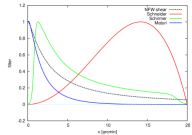
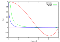
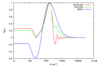
Different filter profiles have been proposed in the literature depending on their specific application in weak-lensing. We adopt three of them here which have been used so far to identify halo candidates through weak lensing.

(1) The polynomial filter described by Schneider et al. (1998)

$$Q_{\rm poly}(x)=\frac{6x^{2}}{\pi r_{\rm s}^{2}}\left(1-x^{2}\right)H\left(1-x\right)\;,$$ (8)

where the projected angular distance from the filter centre, $x=r/r_{\rm s}$, is expressed in units of the filter scale radius, $r_{\rm s}$, and $H$ is the Heaviside step function. This filter was originally proposed for cosmic-shear analysis but several authors have used it also for dark matter halo searches (see for e.g. Erben et al., 2000; Schirmer et al., 2004).

(2) A filter optimised for halos with NFW density profile, approximating their shear signal with a hyperbolic tangent (Schirmer et al., 2004),

$$Q_{\rm tanh}(x)=\left(1+\mathrm{e}^{a-bx}+\mathrm{e}^{cx-d}\right)^{-1}\tanh\left(x/x_{\rm c}\right)\;,$$ (9)

where the two exponentials in parentheses are cut-offs imposed at small and large radii ($a=6$, $b=150$, $c=50$, and $d=47$) and $x_{\rm c}$ is a parameter defining the filter-profile slope. A good choice for the latter is $x_{\rm c}=0.1$ as empirically shown by Hetterscheidt et al. (2005).

(3) The optimal linear filter introduced by Maturi et al. (2005) which, together with the optimisation with respect to the expected halo-lensing signal, optimally suppresses the contamination due to the line-of-sight projection of large-scale structures (LSS),

$$\hat{Q}_{\rm opt}(\@vec{k})=\alpha\frac{\tau(\@vec{k})}{P(k)}\quad\mbox{with}\quad\alpha^{-1}=\int\mathrm{d}^{2}k\frac{\left|\hat{\tau}(\@vec{k})\right|^{2}}{P(k)}\;.$$ (10)

Here, $\hat{\tau}(k)$ is the Fourier transform of the expected shear profile of the halo and $P(k)=P_{\rm g}+P_{\rm LSS}(k)$ is the complete noise power spectrum including the LSS through $P_{\rm LSS}$ and the noise contributions from the intrinsic source ellipticities and the shot noise by $P_{\rm g}=\sigma_{\rm g}^{2}/(2n_{\rm g})$, given their angular number density $n_{\rm g}$ and the intrinsic ellipticity dispersion $\sigma_{\rm g}$. This filter depends on parameters determined by physical quantities such as the halo mass and redshift, the galaxy number density and the intrinsic ellipticity dispersion and not on an arbitrarily chosen scale which has to be determined empirically through costly numerical simulations (e.g. Hennawi & Spergel, 2005). An application of this filter to the GaBoDS survey (Schirmer et al., 2003) was presented in Maturi et al. (2007), while a detailed comparison of these filters was performed by Pace et al. (2007) by means of numerical ray-tracing simulations. They found that the optimal linear filter given by Eq. (10) returns the halo sample with the largest completeness ($100\%$ for masses $M\geq 3\times 10^{14}\,h^{-1}\,M_{\odot}$ and $\sim 50\%$ for masses $M\sim 2\times 10^{14}\,h^{-1}\,M_{\odot}$ for sources at $z_{\mathrm{s}}=1$) and the smallest number of spurious detections caused by the LSS ($\leq 10\%$ for a signal-to-noise threshold of $\mathrm{S/N}\sim 5$).

3.3 Weak lensing estimator and convergence

In order to simplify comparisons with numerical simulations, we convert the estimator $\tilde{A}$ from Eq. (5) to an estimator of the convergence,

$$\tilde{A}(\@vec{\theta}) = \int\mathrm{d}^{2}\theta^{\prime}\kappa(\@vec{\theta}^{\prime})U(|\@vec{\theta}^{\prime}-\@vec{\theta}|)\;,$$ (11)

where $U$ is related to $Q$ by

$$Q(\theta)=\frac{2}{\theta^{2}}\int_{0}^{\theta}\mathrm{d}\theta^{\prime}\theta^{\prime}U(\theta^{\prime})-U(\theta)$$ (12)

(Schneider, 1996) if the weight function $U(\theta)$ is defined to be compensated, i.e.

$$\int\mathrm{d}\theta^{\prime}\theta^{\prime}U(\theta^{\prime})=0\;.$$ (13)

Equation (12) has the form of a Volterra integral equation of the first kind which can be solved with respect to $U$ once $Q$ is specified. If $\lim_{\rm x\rightarrow 0}Q(x)/x$ is finite, the solution is

$$U(\theta)=-Q(\theta)-\int_{0}^{\theta}\mathrm{d}\theta^{\prime}\frac{2}{\theta^{\prime}}Q(\theta^{\prime})\;,$$ (14)

(Polyanin & Manzhirov, 1998) which can be solved analytically for the polynomial filter

$$U_{\rm poly}(x)=\frac{9}{\pi r_{\rm s}^{2}}\left(1-x^{2}\right)\left(\frac{1}{3}-x^{2}\right)H\left(1-x\right)\;,$$ (15)

and numerically for the hyperbolic-tangent filter of Eq. (9) with an efficient recursive scheme over the desired radii $\theta$. If $\lim_{\rm x\rightarrow 0}Q(x)/x=\infty$ as in the case of the optimal filter, Eq. (14) can be solved by introducing an exponential cut-off at small radii to avoid the divergence. The correct solution is obtained if the cut-off scale is close to the mean separation between the background galaxies, so that no information is lost. Alternatively, Eq. (12) can be solved iteratively with respect to $Q$ by

$$U_{0}(\theta)=-Q(\theta)\;,\quad U_{n}(\theta)=-Q(\theta)+\frac{2}{\theta^{2}}\int_{0}^{\theta}\mathrm{d}\theta^{\prime}\theta^{\prime}U_{n-1}(\theta)\;.$$ (16)

The iterative procedure is stopped once the difference $U_{n}(\theta)-U_{n-1}(\theta)$ is sufficiently small. After $U(\theta)$ has been found, an appropriate constant $c$ has to be added in order to satisfy the compensation requirement, Eq. (13). It is given by

$$c=-\frac{2}{\theta_{\mathrm{max}}^{2}}\int\limits_{0}^{\theta_{\mathrm{max}}}\mathrm{d}\theta^{\prime}\theta^{\prime}U(\theta^{\prime})\;.$$ (17)

We show in Fig. (1) the resulting filter profiles to be used on shear catalogues through Eq. (5) and their corresponding variants to be used on convergence fields with Eq. (11) both in real and Fourier space. All of them are band-pass filters and the two of them designed for halo searches have larger amplitudes at higher frequencies compared to the polynomial filter by Schneider et al. (1998), where the halo signal is most significant. This feature is particularly prominent for the optimal filter, which is additionally negative at low frequencies, where the LSS signal dominates. These two features ensure the minimisation of the LSS contamination in halo searches.

4 Predicting weak lensing peak counts

Our analytic predictions for the number counts of weak-lensing detections as a function of their signal-to-noise ratio are based on modelling the analysed lensing data, resulting from Eq. (11), as an isotropic and homogeneous Gaussian random field. This is an extremely good approximation for the noise and the LSS components, but not for the non-linear structures such as sufficiently massive halos, as we shall discuss in Sec. 5.3.

4.1 Statistics of Gaussian random fields

An $n$-dimensional random field $F(\@vec{r})$ assigns a set of random numbers to each point $\@vec{r}$ in an $n$-dimensional space. A joint probability function can be declared for $m$ arbitrary points $\@vec{r}_{j}$ as the probability to have field values between $F(\@vec{r}_{j})$ and $F(\@vec{r}_{j})+{\rm d}F(\@vec{r}_{j})$, with $j=1,\ldots,m$. For Gaussian random fields, the field itself, its derivatives, integrals and any linear combination thereof are Gaussian random variables which we denote by $y_{i}$ with mean value $\langle y_{i}\rangle$ and central deviations $\Delta y_{i}:=y_{i}-\langle y_{i}\rangle$, with $i=1,\ldots,p$. Their joint probability function is a multivariate Gaussian,

$$\mathcal{P}(y_{1},\ldots,y_{\rm p})\,{\rm d}y_{1}\cdots{\rm d}y_{\rm p}=\frac{1}{\sqrt{\left(2\pi\right)^{p}\det\left(\@tens{\mathcal{M}}\right)}}\,{\rm e}^{-\mathcal{Q}}\,{\rm d}y_{1}\cdots{\rm d}y_{\rm p}$$ (18)

with the quadratic form

$$\mathcal{Q}:=\frac{1}{2}\sum_{\rm i,j=1}^{p}\Delta y_{\rm i}\left(\@tens{\mathcal{M}}^{-1}\right)_{\rm ij}\Delta y_{\rm j}\;,$$ (19)

where $\@tens{\mathcal{M}}$ is their covariance matrix with elements $\mathcal{M}_{ij}:=\langle\Delta y_{i}\Delta y_{j}\rangle$. All statistical properties of a homogeneous Gaussian random field with zero mean are fully characterised by the two-point correlation function $\zeta(\@vec{r}_{1},\@vec{r}_{2})=\zeta(|\@vec{r}_{1}-\@vec{r}_{2}|):=\langle F(\@vec{r}_{1})F(\@vec{r}_{2})\rangle$ or equivalently its Fourier transform, the power spectrum $P(k)$. In our case, this is the sum of the matter fluctuation convergence power spectrum, $P_{\rm LSS}(k)$, and observational noise, $P_{\rm n}(k)$.

Since we are interested in gravitational-lensing quantities such as the convergence $\kappa$, we here consider two-dimensional Gaussian random fields only. We adopt the formalism of Bardeen et al. (1986), where $F=\kappa$, $\eta_{i}=\partial_{i}F$ and $\zeta_{ij}=\partial_{i}\partial_{j}F$ denote the convergence field and its first and second derivatives, respectively.

4.2 Definition of detections: a new up-crossing criterion

We define as detection any contiguous area of the field $\kappa$ which exceeds a given threshold, $\kappa_{\mathrm{th}}=\mbox{S/N}\cdot\sigma_{\tilde{A}}$, determined by the required signal-to-noise ratio, S/N, and the variance $\sigma_{\tilde{A}}$ of an estimator $\tilde{A}$ (see Eq. 7). This definition is widely used in surveys for galaxy clusters or peak counts in weak-lensing surveys and can easily be applied both to real data and Gaussian random fields.

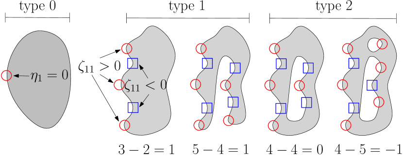
Each detection is delimited by its contour at the threshold level $\kappa_{\mathrm{th}}$. If this contour is approximately circular, it has a single point $\@vec{r}_{\mathrm{up}}$, called up-crossing point, where the field is rising along the x-axis direction only, i.e. where the field gradient has one vanishing and one positive component (see the sketch for type-0 detections in the lower panel of Fig. 2),

$$F(\@vec{r}_{\mathrm{up}})=\kappa_{\mathrm{th}}\;,\quad\eta_{1}(\@vec{r}_{\mathrm{up}})=0\;,\quad\eta_{2}(\@vec{r}_{\mathrm{up}})>0\;.$$ (20)

Since we assume $\kappa$ to be a homogeneous and isotropic random field, the orientation of the coordinate frame is arbitrary and irrelevant. The conditions expressed by Eq. (20) define the so-called up-crossing criterion which allows to identify the detections and to derive their statistical properties, such as their number counts, by associating their definition to the Gaussian random field variables $F$, $\eta_{1}$ and $\eta_{2}$.

However, this criterion is prone to fail for low thresholds, where detections tend to merge and the isocontours tend to deviate from the assumed approximately circular shape. This causes detection numbers to be overestimated at low cut-offs because each “peninsula” and “bay” of their profile (see type-1 in Fig. 2) would be counted as one detection. We solve this problem by dividing the up-crossing points into those with positive (red circles) and those with negative (blue squares) curvature, $\zeta_{11}>0$ and $\zeta_{11}<0$ respectively. In fact, for each detection, their difference is one (type-1) providing the correct number count. The only exception is for those detections containing one or more “lagoons” (type-2) since each of them decreases the detection count by one. But since this is not a frequent case and occurs only at very low cut-off levels, we do not consider this case here.

Figure 2: Weak lensing detection maps. The top four panels show the segmentation of a realistic weak-lensing S/N map for increasing thresholds: 0.1, 0.5, 1, and 2, respectively. The bottom panel sketches the three discussed detections types together with the points identified by the standard and the modified up-crossing criteria. Red circles and blue squares correspond to up-crossing points for which the second field derivatives are $\zeta_{11}>0$ and $\zeta_{11}<0$, respectively.

4.3 The number density of detections

Once the relation between the detections and the Gaussian random variables $\@vec{y}=(\kappa_{\rm th},\eta_{1},\eta_{2},\zeta_{11})$ and their constraints from Eq. (20) together with $\zeta_{11}>0$ or $\zeta_{11}<0$ are defined, we can describe their statistical properties through the multivariate Gaussian probability distribution given by Eq. (18) with the covariance matrix

$$\@tens{\mathcal{M}}=\left(\begin{array}[]{cccc}\sigma_{0}^{2}&0&0&-\sigma_{1}^{2}/2\\ 0&\sigma_{1}^{2}/2&0&0\\ 0&0&\sigma_{1}^{2}/2&0\\ -\sigma_{1}^{2}/2&0&0&3\sigma_{2}^{2}/8\\ \end{array}\right)\;.$$ (21)

This matrix differs from that derived by Bardeen et al. (1986) and Angrick & Bartelmann (2009) because we are dealing with a 2-dimensional rather than a 3-dimensional field. Here, the $\sigma_{j}$ are the moments of the power spectrum $P(k)$

$$\sigma_{j}^{2}=\int\frac{k^{2j+1}\,\mathrm{d}k}{2\pi}P(k)\hat{W}^{2}(k)|\hat{Q}(k)|^{2}\;,$$ (22)

where $\hat{W}(k)$ is the frequency response of the survey given by its geometry (see Sec. 5.2) and $\hat{Q}(k)$ is the Fourier transform of the filter adopted for the weak lensing estimator (see Sec. 3.2). The determinant of $\@tens{\mathcal{M}}$ is $(3\sigma_{0}^{2}\sigma_{1}^{4}\sigma_{2}^{2}-2\sigma_{1}^{8})/32$ and Eq. (19) can explicitly be written as

$$\mathcal{Q}=\frac{1}{2}\left(\frac{2\@vec{\eta}^{2}}{\sigma_{1}^{2}}+\frac{8\zeta_{11}^{2}\sigma_{0}^{2}+8\zeta_{11}\kappa\sigma_{1}^{2}+3\kappa^{2}\sigma_{2}^{2}}{3\sigma_{0}^{2}\sigma_{2}^{2}-2\sigma_{1}^{4}}\right)\;.$$ (23)

Both $\kappa$ and $\eta_{1}$ can be expanded into Taylor series around the points $\@vec{r}_{\mathrm{up}}$ where the up-crossing conditions are fulfilled,

$$\kappa(\@vec{r})\approx\kappa_{\mathrm{th}}+\sum_{i=1}^{2}\eta_{i}(\@vec{r}-\@vec{r}_{\mathrm{up}})_{i}\;,\quad\eta_{1}(\@vec{r})\approx\sum_{i=1}^{2}\zeta_{1i}(\@vec{r}-\@vec{r}_{\mathrm{up}})_{i}\;,$$ (24)

so that the infinitesimal volume element $\mathrm{d}\kappa\mathrm{d}\eta_{1}$ can be written as $\mathrm{d}\kappa\mathrm{d}\eta_{1}=|\det\@tens{J}|\mathrm{d}^{2}r$, where $\@tens{J}$ is the Jacobian matrix,

$$\@tens{J}=\left(\begin{array}[]{cc}\partial\kappa/\partial x_{1}&\partial\kappa/\partial x_{2}\\ \partial\eta_{1}/\partial x_{1}&\partial\eta_{1}/\partial x_{2}\\ \end{array}\right)=\left(\begin{array}[]{cc}\eta_{1}&\eta_{2}\\ \zeta_{11}&\zeta_{12}\\ \end{array}\right)$$ (25)

and $|\det\@tens{J}|=|\eta_{2}\zeta_{11}|$ since $\eta_{1}=0$. The number density of up-crossing points at the threshold $\kappa_{\mathrm{th}}$ with $\zeta_{11}>0$, and $\zeta_{11}<0$, $n^{+}$ and $n^{-}$ respectively, can thus be evaluated as

$$n^{\pm}(\kappa_{\mathrm{th}})=\pm\int\limits_{0}^{\infty}\mathrm{d}\eta_{2}\int\limits_{0}^{\infty}\mathrm{d}\zeta_{11}|\eta_{2}\zeta_{11}|\,\mathcal{P}\left(\kappa=\kappa_{\mathrm{th}},\eta_{1}=0,\eta_{2},\zeta_{11}\right)\,,$$ (26)

where $\mathcal{P}(\kappa,\eta_{1},\eta_{2},\zeta_{11})$ is the multivariate Gaussian defined by Eq. (18) with $p=4$, the correlation matrix (21), and the quadratic form (23). Both expressions can be integrated analytically and their difference, $n_{\mathrm{det}}(\kappa_{\mathrm{th}})=n^{+}(\kappa_{\mathrm{th}})-n^{-}(\kappa_{\mathrm{th}})$, as explained in Sect. 4.2, returns the number density of detections $n_{\mathrm{det}}$ above the threshold $\kappa_{\mathrm{th}}$,

$$n_{\mathrm{det}}(\kappa_{\mathrm{th}})=\frac{1}{4\sqrt{2}\pi^{3/2}}\left(\frac{\sigma_{1}}{\sigma_{0}}\right)^{2}\frac{\kappa_{\mathrm{th}}}{\sigma_{0}}\exp\left(-\frac{\kappa_{\mathrm{th}}^{2}}{2\sigma_{0}^{2}}\right)\;.$$ (27)

Note how the dependence on $\sigma_{2}$ drops out of the difference $n^{+}-n^{-}$, leading to a very simple result.

For completeness we report the number density estimate also for the classical up-crossing criterion, Eq. (20) only, where the constraint on the second derivative of the field, $\zeta_{11}$, is not used,

$$n_{\mathrm{up}}(\kappa_{\mathrm{th}}) = \frac{1}{4\sqrt{2}\pi^{2}\sigma_{0}}\left(\frac{\sigma_{1}}{\sigma_{0}}\right)^{2}\exp\left(-\frac{\kappa_{\mathrm{th}}^{2}}{2\sigma_{0}^{2}}\right)$$

$$\times \left[\exp\left(-\frac{\kappa_{\mathrm{th}}^{2}\sigma_{1}^{4}}{\sigma_{0}^{2}\gamma^{2}}\right)\sigma_{0}\gamma+\sqrt{\pi}\kappa_{\mathrm{th}}\,\mathrm{erf}\left(\frac{\kappa_{\mathrm{th}}\sigma_{1}^{2}}{\sigma_{0}\gamma}\right)\right]\;,$$

with $\gamma:=\sqrt{3\sigma_{0}^{2}\sigma_{2}^{2}-2\sigma_{1}^{4}}$. This number density converges to the correct value $n_{\mathrm{det}}$ for $\kappa_{\mathrm{th}}\rightarrow\infty$, i.e. large thresholds, because $\mathrm{erf}(x)\rightarrow 1$ and $\exp(-x^{2})\rightarrow 0$. This reflects the fact that, for large thresholds, the detection shapes become fully convex and any issues with more complex shapes disappear.

5 Analytic predictions vs. numerical simulations

We now compare the number counts of detections predicted by our analytic approach with those resulting form the analysis of synthetic galaxy catalogues produced with numerical ray-tracing simulations.

Figure 3: Comparison between the power spectrum measured from the analysis of shear catalogues derived from numerical simulations (heavy line) and the prediction resulting from the Peacock & Dodds (1996) power spectrum convolved with the survey frequency response and the adopted filter. We show from top to bottom the results for the polynomial filter with $r_{s}=5\aas@@fstack{\prime}5$, the hyperbolic-tangent filter with $r_{s}=10^{\prime}$ and the optimal filter with the cluster model scale radius set to $r_{s}=1^{\prime}$.

5.1 Numerical simulations

We use a hydrodynamical, numerical $N$-body simulation carried out with the code GADGET-2 (Springel, 2005). We briefly summarise its main characteristics here and refer to Borgani et al. (2004) for a more detailed discussion. The simulation represents a concordance $\Lambda$CDM model, with dark-energy, dark-matter and baryon density parameters $\Omega_{\Lambda}=0.7$, $\Omega_{\rm m}=0.3$ and $\Omega_{\rm b}=0.04$, respectively. The Hubble constant is $H_{0}=100\,h\,\mathrm{km\,s^{-1}\,Mpc^{-1}}$ with $h=0.7$, and the linear power spectrum of the matter-density fluctuations is normalised to $\sigma_{8}=0.8$. The simulated box is a cube with a side length of $192\,h^{-1}$Mpc, containing $480^{3}$ dark-matter particles with a mass of $6.6\times 10^{9}\,h^{-1}M_{\odot}$ each and an equal number of gas particles with $8.9\times 10^{8}\,h^{-1}M_{\odot}$ each. Thus, halos of mass $10^{13}\,h^{-1}M_{\odot}$ are resolved into several thousands of particles. The physics of the gas component includes radiative cooling, star formation and supernova feedback, assuming zero metallicity.

This simulation is used to construct backward light cones by stacking the output snapshots from $z=1$ to $z=0$. Since the snapshots contain the same cosmic structures at different evolutionary stages, they are randomly shifted and rotated to avoid repetitions of the same cosmic structures along one line-of-sight. The light cone is then sliced into thick planes, whose particles are subsequently projected with a triangular-shaped-cloud scheme (TSC, Hockney & Eastwood, 1988) on lens planes perpendicular to the line-of-sight. We trace a bundle of $2048\times 2048$ light rays through the light cone which start propagating at the observer into directions on a regular grid of $4.9$ degrees on each side. The effective resolution of this ray-tracing simulation is of $1^{\prime}$ (for further detail, see Pace et al., 2007).

The effective convergence and shear maps obtained from the ray-tracing simulations are used to lens a background source population according to Eq. (4). Galaxies are randomly distributed on the lens plane at $z=1$ with a number density of $n_{\rm g}=30$ arcmin^-2 and have intrinsic random ellipticities drawn from the distribution

$$p(\epsilon_{\rm s})=\frac{\exp{|(1-|\epsilon_{\rm s}|^{2})/\sigma_{\epsilon}^{2}|}}{\pi\sigma_{\epsilon}^{2}|\exp{(1/\sigma_{\epsilon}^{2})}-1|}\;,$$ (29)

where $\sigma_{\epsilon}=0.25$.

Synthetic galaxy catalogues produced in this way are finally analysed with the aperture mass (Eq. 5) evaluated on a regular grid of $512\times 512$ positions covering the entire field-of-view of the light cone. All three filters presented in § 3.2 were used with three different scales: the polynomial filter with $r_{\rm s}=2\aas@@fstack{\prime}75,\ 5\aas@@fstack{\prime}5,$ and $11^{\prime}$, the hyperbolic-tangent filter with $r_{\rm s}=5^{\prime},\ 10^{\prime},$ and $20^{\prime}$, and the optimal filter with scale radii of the cluster model set to $r_{s}=1^{\prime},\ 2^{\prime},$ and $4^{\prime}$. These scales are chosen such that the effective scales of the different filters can be compared. For a statistical analysis of the weak-lensing detections and their relation to the numerical simulations structures, see Pace et al. (2007).

Figure 4: Number of peaks detected in the numerical simulation (shaded area) compared to the prediction obtained with the proposed method both with the original up-crossing criterion (dashed line) and with the new blended up-crossing criterion (points with error bars). The standard up-crossing criterion is a good approximation for high signal-to-noise ratios but fails for lower S/N, which are well described by the new version.

5.2 Accounting for the geometry of surveys: the window function

Our analytic predictions for the number density of detections accounts for the full survey geometry, through the frequency response $\hat{W}(k)$ in Eq. (22). Any survey geometry can be considered but, for sake of simplicity, we evaluate our estimates for a square-shaped field-of-view without gaps. Under these assumptions, the frequency response, $W(k)$, is the product of a high-pass filter suppressing the scales larger than the light cone’s side length $L_{\rm f}=2\pi/k_{\mathrm{f}}=4.9\;\mbox{deg}$,

$$\hat{W}^{2}_{\mathrm{f}}(k)=\exp\left(-\frac{k_{\mathrm{f}}^{2}}{k^{2}}\right)\;,$$ (30)

a low-pass filter imposed by the average separation $d=2\pi/k_{\rm g}=n_{\rm g}^{-1/2}=0\aas@@fstack{\prime}18$ between the galaxies,

$$\hat{W}_{\mathrm{g}}^{2}(k)=\exp\left(-\frac{k^{2}}{k_{\mathrm{g}}^{2}}\right)\;,$$ (31)

and a low-pass filter related to the resolution $R_{\mathrm{pix}}=0\aas@@fstack{\prime}57$ used to sample the sky with the weak lensing estimator $\tilde{A}$ of Eq. (5),

$$\hat{W}_{\mathrm{pix}}^{2}(k)=\frac{2\,\sqrt{\pi}}{kR_{\mathrm{pix}}}\,\mathrm{J}_{1}\left(\frac{kR_{\mathrm{pix}}}{\sqrt{\pi}}\right)\;,$$ (32)

where $\mathrm{J}_{1}(x)$ is the cylindrical Bessel function of order one. The latter function is a circular step function covering the same area as a square-shaped pixel of size $R_{\mathrm{pix}}$. The square shapes of the field-of-view and the pixels could be better represented by the product of two step functions in both the $x$- and $y$-direction, but the low gain in accuracy does not justify the higher computational cost. Finally, for the comparison with our numerical ray-tracing simulation, we have to account for its resolution properties which act on the convergence power spectrum only by convolving $P_{\kappa}$ with a low-pass filter

$$\hat{W}_{\mathrm{s}}^{2}(k)=\exp\left(-\frac{k^{2}}{k_{\mathrm{s}}^{2}}\right)\;,$$ (33)

where $k_{\mathrm{s}}=2\pi/1\;\mbox{arcmin}^{-1}$ as discussed in § 5.1.

Note that when relating the detection threshold to the signal-to-noise ratio S/N according to the estimator variance using Eq. (7) and $\kappa_{\mathrm{th}}=\mbox{S/N}\cdot\sigma_{\tilde{A}}$, all filters mentioned are used except for $\hat{W}_{\rm pix}$, which, of course, does not affect the estimator variance.

5.3 Comparison with numerical simulations

Figure 5: Number of weak lensing peaks, shown as a function of the signal-to-noise ratio, predicted with the analytic method presented here for the Schneider et al. (1998), the Schirmer et al. (2004) and the Maturi et al. (2005) filters from top to bottom, and increasing filter radii from left to right. The number counts generated by the intrinsic galaxy noise alone, $P_{\rm g}$, and the LSS alone, $P_{\rm LSS}$, are also shown. Numbers refer to a survey of one square degree with a galaxy number density of $n_{\rm g}=30\ \mbox{arcmin}^{-1}$ and an intrinsic shear dispersion of $\sigma_{\rm g}=0.25$. The results are compared with the number counts of positive as well as negative peaks detected based on the synthetic galaxy catalogues from the numerical simulation.

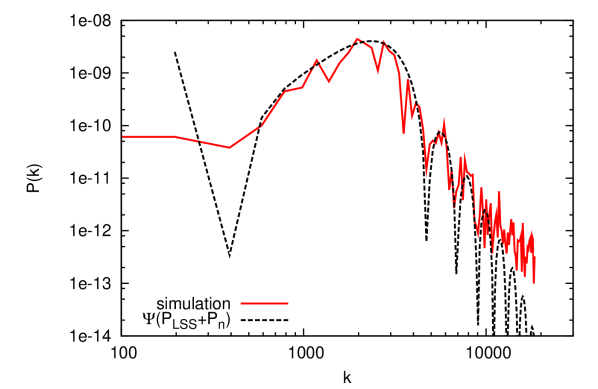
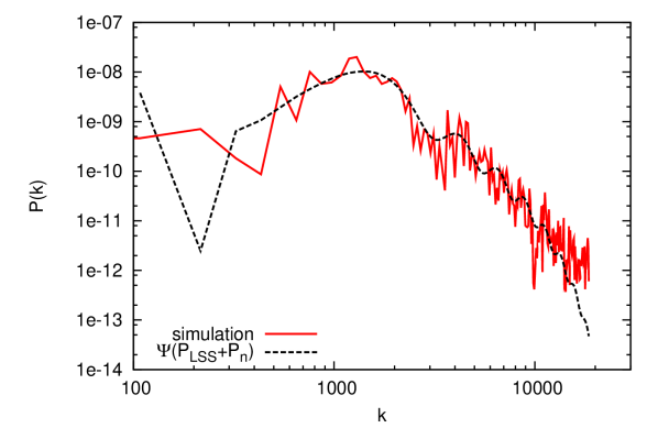
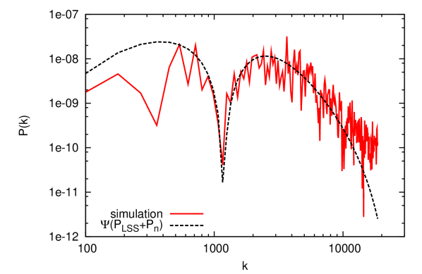
We first compare in Fig. 3 the expected filtered power spectra for the convergence and the intrinsic noise of the galaxies, $P|\hat{W}\hat{Q}|^{2}$, assumed in Eq. (22), with those measured from the analysed synthetic galaxy catalogue. All main features are very well reproduced. Only at high frequencies the assumed power spectra drop slightly more steeply than measured in the numerical simulations.

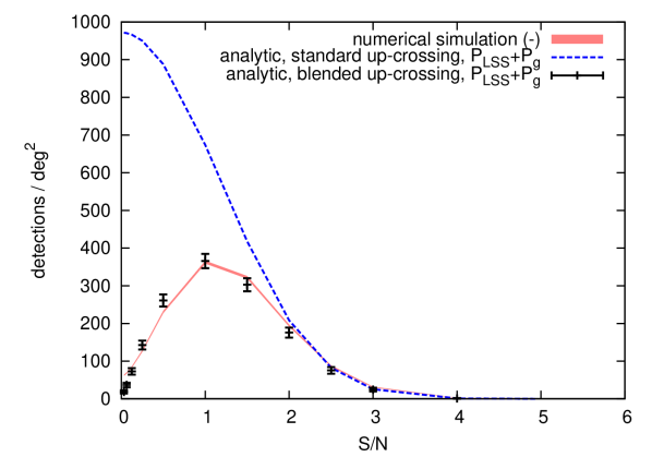
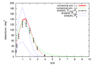
A comparison of the original up-crossing criterion with the new blended up-crossing criterion presented here is shown in Fig. 4 together with the number counts obtained from the numerical simulations. Only the result for the optimal filter with $r_{\rm s}=1^{\prime}$ is shown for clarity. As expected, the two criteria agree very well for high signal-to-noise ratios since the detections are mostly of type-0, i.e. approximately circular, as shown in the left panel of Fig. 2, while the merging of detections at lower signal-to-noise ratios is correctly taken into account only by our new criterion. Note that our analytic approach approximates the data as random Gaussian fields, very well representing noise and LSS but not non-linear objects such as galaxy clusters. Thus, particular care has to be taken when comparing the predicted number counts with real or simulated data by modelling the non-linear structures, which is difficult and uncertain, or by avoiding their contribution in first place. We follow the latter approach by counting the negative instead of the positive peaks found in the galaxy catalogues. In fact, massive halos contribute only positive detections in contrast to the LSS and other sources of noise which equally produce positive and negative detections with the same statistical properties.

This is an interesting application for cosmology, where a robust prediction of number counts in the linear regime only can be directly compared to data or, turning the argument around, can be used to statistically correct the halo number counts by using the data only. In fact, the difference of the positive and negative detection counts is caused by non linear structures only and their Poisson fluctuations.

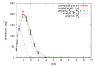
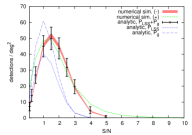
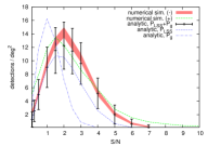
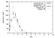
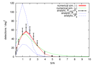
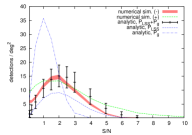
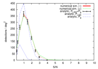
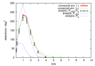
Our analytic predictions for all filters and both positive and negative detection counts resulting from the synthetic galaxies catalogue from the numerical simulation are shown in Fig. 5. The high signal-to-noise ratio tail caused by the nonlinear structures is present only in the positive detection counts, as expected. The agreement with the negative detections is within the 1-$\sigma$ error bars (considering the uncertainties for a one square degree survey) except for Schirmer et al. (2004) filter and the optimal filter, both with a scale of 5 arcmin, which are compatible only at a 2-$\sigma$ level. It is plausible that these small deviations are caused by the ignored correlation between the pixels which, in the noise evaluation, are treated as independent. The filter radii are in fact larger than the pixel separation, so that different pixels have some common galaxies.

We finally compare the contribution of the LSS and the noise to the total signal by treating them separately. Their number counts are plotted with dashed lines in Fig. 5. All filters show an unsurprisingly large number of detections caused by the noise up to signal-to-noise rations of 3 and a number of detections caused by the LSS increasing with the filter scale except for the optimal filter, which always suppresses their contribution to a negligible level. Thus, the LSS contaminates halo catalogues selected by weak lensing up to signal-to-noise ratios of $4-5$ if its contribution is ignored in the filter definition. Note that the total number of detections can be obtained only by counting the peaks from the total signal, i.e. LSS plus noise, and not by adding the peaks found in the two components separately, because the blending of peaks is different for the two cases.

6 Conclusion

We have developed an analytic method for predicting peak counts in weak-lensing surveys, based on the theory of Gaussian random fields (Bardeen et al., 1986). Peaks are typically detected in shear fields after convolving them with filters of different shapes and widths. We have taken these into account by first filtering the assumed Gaussian random field appropriately and then searching for suitably defined peaks. On the way, we have argued for a refinement of the up-crossing criterion for peak detection which avoids biased counts of detections with low signal-to-noise ratio, and implemented it in the analytic peak-count prediction. Peaks in the non-linear tail of the shear distribution are underrepresented in this approach because they are highly non-Gaussian, but our method is well applicable to the prediction of spurious counts, and therefore to the quantification of the background in attempts to measure number densities of dark-matter halos. We have compared our analytic prediction to peak counts in numerically simulated, synthetic shear catalogues and found agreement at the expected level.

Our main results can be summarised as follows:

• The shape and size of the filter applied to the shear field has a large influence on the contamination by spurious detections. For the optimal filter, the contribution by large-scale structures is low on all filter scales, while they typically contribute substantially for other filters.

• Shape and shot noise due to the background galaxies used to measure the shear from are a large source of spurious peak counts for all filters, and the dominant source for the optimal filter.

• Taken together, large-scale structure and galaxy noise contribute the majority of detections up to signal-to-noise ratios between 3–5. Only above this level, detections due to real dark-matter halos begin dominating.

• The optimal filter allows the detection of $\sim$30–40 halos per square degree at signal-to-noise ratios high enough for suppressing all noise contributions. For the other filters, this number is lower by almost an order of magnitude.

Our conclusions are thus surprisingly drastic: peak counts in weak-lensing surveys are almost exclusively caused by chance projections in the large-scale structure and by galaxy shape and shot noise unless only peaks with high signal-to-noise ratios are counted. With typical filters, only a few detections per square degree can be expected at that level, while the optimal filter returns up to an order of magnitude more.

Appendix A Forecast for different weak lensing surveys

For convenience, we evaluate here the expected number density of peak counts for a collection of present and future weak-lensing surveys. To give typical values, we assumed for all of them a square-shaped field of view, a uniform galaxy number density and no gaps for two main reasons. First, their fields-of-view are typically very large and thus do not affect the frequencies relevant for our evaluation. Second, the masking of bright objects can be done in many different ways which cannot be considered in this paper in any detail. Finally we fixed the sampling scale, described by Eq. (32), to be 5 times smaller than the typical filter scale in order to avoid undersampling, i.e. such that the high frequency cut-off is imposed by the filters themselves. The results are shown in Tab. 1 together with the number counts obtained with a simple Gaussian filter, usually used together with the Kaiser & Squires shear inversion algorithm (Kaiser & Squires 1993).

Table 1: Expected number counts of peak detections per square degree for $\mathrm{S/N}=1,3,5$ and for several present and future weak-lensing surveys with different intrinsic ellipticity dispersion, $\sigma_{\epsilon}$, and galaxy number density, $n_{\rm g}$, per arcmin². For each filter, we used three different scales, namely $Q_{poly}$: scale-1=$2\aas@@fstack{\prime}75$, scale-2=$5\aas@@fstack{\prime}5$, scale-3=$11^{\prime}$; $Q_{tanh}$: scale-1=$5^{\prime}$, scale-2=$10^{\prime}$, scale-3=$20^{\prime}$; $Q_{opt}$: scale-1=$10^{14}\,\mathrm{M}_{\odot}$ and scale-2=$5\times 10^{14}\,\mathrm{M}_{\odot}$. $Q_{gaus}$ (Gaussian FWHM): scale-1=$1^{\prime}$, scale-2=$2^{\prime}$, scale-3=$5^{\prime}$.

Pan-STARRS	$Q_{poly}$			$Q_{tanh}$			$Q_{opt}$			$Q_{gaus}$
$\sigma_{\epsilon}=0.3$, $n_{\rm g}=5$	1	3	5	1	3	5	1	3	5	1	3	5
scale-1	207.7	8.127	0.002	252.7	8.824	0.002	186.3	6.243	0.001	3125	131.1	0.042
scale-2	51.49	2.82	0.001	61.8	3.214	0.002	62.69	3.576	0.002	989.6	38.93	0.011
scale-3	12.45	1.258	0.002	14.02	1.518	0.003	-	-	-	173.2	7.82	0.003
DES	$Q_{poly}$			$Q_{tanh}$			$Q_{opt}$			$Q_{gaus}$
$\sigma_{\epsilon}=0.3$, $n_{\rm g}=10$	1	3	5	1	3	5	1	3	5	1	3	5
scale-1	206.6	9.55	0.004	248.9	10.98	0.004	288.8	12.72	0.005	3593	144.5	0.043
scale-2	50.09	4.178	0.005	56.87	5.112	0.008	95.6	8.325	0.012	1047	41.67	0.012
scale-3	11.67	2.339	0.0174	11.92	2.847	0.030	-	-	-	169.8	9.807	0.006
CFHTLS	$Q_{poly}$			$Q_{tanh}$			$Q_{opt}$			$Q_{gaus}$
$\sigma_{\epsilon}=0.3$, $n_{\rm g}=20$	1	3	5	1	3	5	1	3	5	1	3	5
scale-1	206.6	9.907	0.004	249.6	11.48	0.004	324	14.12	0.005	3971	151.6	0.041
scale-2	49.76	4.545	0.007	55.86	5.61	0.010	104.5	9.519	0.015	1085	42.15	0.012
scale-3	11.49	2.622	0.025	11.51	3.166	0.044	-	-	-	169.7	10.28	0.007
Subaru	$Q_{poly}$			$Q_{tanh}$			$Q_{opt}$			$Q_{gaus}$
$\sigma_{\epsilon}=0.3$, $n_{\rm g}=30$	1	3	5	1	3	5	1	3	5	1	3	5
scale-1	198.5	16.22	0.020	219.5	21.51	0.038	603.2	42.99	0.04045	4110	160.9	0.046
scale-2	44.84	10.82	0.117	42.97	13.32	0.237	172.8	29.81	0.1642	1070	50.42	0.021
scale-3	9.406	6.321	0.528	7.857	6.457	0.807	-	-	-	151.6	19.14	0.057
EUCLID	$Q_{poly}$			$Q_{tanh}$			$Q_{opt}$			$Q_{gaus}$
$\sigma_{\epsilon}=0.3$, $n_{\rm g}=40$	1	3	5	1	3	5	1	3	5	1	3	5
scale-1	194.3	20.01	0.039	206.3	27.29	0.088	730.9	58.61	0.070	4189	165.5	0.048
scale-2	42.64	14.25	0.295	38.54	16.8	0.591	197.7	40.75	0.321	1062	54.99	0.027
scale-3	8.653	7.642	1.104	6.873	7.282	1.514	-	-	-	143.6	24.19	0.127
LSST	$Q_{poly}$			$Q_{tanh}$			$Q_{opt}$			$Q_{gaus}$
$\sigma_{\epsilon}=0.22$, $n_{\rm g}=50$	1	3	5	1	3	5	1	3	5	1	3	5
scale-1	174.8	42.42	0.463	156.8	56.13	1.333	1206	138	0.334	4169	187.7	0.070
scale-2	34.5	28.13	3.464	26.15	26.81	5.218	269.2	95.09	2.198	991.5	82	0.104
scale-3	6.403	10.32	4.964	4.519	8.139	4.889	-	-	-	113.5	48.96	1.688
SNAP	$Q_{poly}$			$Q_{tanh}$			$Q_{opt}$			$Q_{gaus}$
$\sigma_{\epsilon}=0.3$, $n_{\rm g}=100$	1	3	5	1	3	5	1	3	5	1	3	5
scale-1	172.6	45.42	0.5824	152.5	59.33	1.664	1322	148.6	0.3481	4287	190.2	0.069
scale-2	33.73	29.39	4.133	25.22	27.43	6.009	281.6	102.2	2.494	991.3	85.32	0.117
scale-3	6.218	10.41	5.403	4.355	8.1	5.19	-	-	-	110.8	51.68	2.083