ITP-SB-09-14

Threshold Resummation for Di-hadron Production
in Hadronic Collisions

Leandro G. Almeidaa𝑎{}^{\,a},   George Stermana𝑎{}^{\,a},   Werner Vogelsangb𝑏{}^{\,b}
a𝑎{}^{a}\,C.N. Yang Institute for Theoretical Physics, Stony Brook University, Stony Brook, New York 11794 – 3840, U.S.A.

b𝑏{}^{b}\,Physics Department, Brookhaven National Laboratory, Upton, NY 11973, U.S.A.

Abstract

We study the resummation of large logarithmic perturbative corrections to the partonic cross sections relevant for di-hadron production in hadronic collisions, H1H2h1h2Xsubscript𝐻1subscript𝐻2subscript1subscript2𝑋H_{1}H_{2}\rightarrow h_{1}h_{2}X, at high invariant mass of the produced hadron pair. These corrections arise near the threshold for the partonic reaction and are associated with soft-gluon emission. We perform the resummation to next-to-leading logarithmic accuracy, and show how to incorporate consistently cuts in rapidity and transverse momentum of the observed particles. We present numerical results for fixed-target and ISR regimes and find enhancements over the next-to-leading order cross section, which significantly improve the agreement between theoretical predictions and data.

1 Introduction

Cross sections for hadron production in hadronic collisions play an important role in QCD. They offer a variety of insights into strong interaction dynamics. At sufficiently large momentum transfer in the reaction, QCD perturbation theory can be used to derive predictions. The cross section may be factorized at leading power in the hard scale into convolutions of long-distance factors representing the structure of the initial hadrons and the fragmentation of the final-state partons into the observed hadrons, and parts that are short-distance and describe the hard interactions of the partons. If the parton distribution functions and fragmentation functions are known from other processes, especially deeply-inelastic scattering and e+esuperscript𝑒superscript𝑒e^{+}e^{-} annihilation, hadron production in hadronic collisions directly tests the factorized perturbative-QCD approach and the relevance of higher orders in the perturbative expansion.

Much emphasis in both theory and experiment has been on single-inclusive hadron production, H1H2hXsubscript𝐻1subscript𝐻2𝑋H_{1}H_{2}\rightarrow hX [1, 2, 3, 4, 5, 6, 7, 8]. Here the large momentum transfer is provided by the high transverse momentum of the observed hadron. Of equal importance, albeit explored to a somewhat lesser extent, is di-hadron production, H1H2h1h2Xsubscript𝐻1subscript𝐻2subscript1subscript2𝑋H_{1}H_{2}\rightarrow h_{1}h_{2}X, when the pair is produced with large invariant mass M𝑀M. In many ways, one may think of this process as a generalization of the Drell-Yan process to a completely hadronic situation, with the Drell-Yan lepton pair replaced by the hadron pair. The process is therefore particularly interesting for studying QCD dynamics, as we shall also see throughout this paper. Experimental data for di-hadron production as a function of pair mass are available from various fixed-target experiments [9, 10, 11], as well as from the ISR [12]. On the theory side, next-to-leading order (NLO) calculations for this process are available [13, 14, 15]. They have been confronted with the available data sets, and it was found that overall agreement could only be achieved when rather small renormalization and factorizations scales were chosen. The NLO calculations in fact show very large scale dependence. If more natural scales are chosen, NLO theory significantly underpredicts the cross section data, as we shall also confirm below.

In the present paper, we investigate the all-order resummation of large logarithmic corrections to the partonic cross sections. This is of considerable interest for the comparison between data and the NLO calculation just described. A related resummation for the single-inclusive hadron cross section [5] was found to lead to significant enhancements of the predicted cross section over NLO, in much better overall agreement with the available data in that case.

At partonic threshold, when the initial partons have just enough energy to produce two partons with high invariant pair mass (which subsequently fragment into the observed hadron pair), the phase space available for gluon bremsstrahlung vanishes, resulting in large logarithmic corrections. To be more specific, if we consider the cross section as a function of the partonic pair mass m^^𝑚\hat{m}, the partonic threshold is reached when s^=m^2^𝑠superscript^𝑚2\hat{s}=\hat{m}^{2}, that is, τ^m^2/s^=1^𝜏superscript^𝑚2^𝑠1\hat{\tau}\equiv\hat{m}^{2}/\hat{s}=1, where s^^𝑠\sqrt{\hat{s}} is the partonic center-of-mass system (c.m.s.) energy. The leading large contributions near threshold arise as αsk[ln2k1(1τ^)/(1τ^)]+superscriptsubscript𝛼𝑠𝑘subscriptdelimited-[]superscript2𝑘11^𝜏1^𝜏\alpha_{s}^{k}\left[\ln^{2k-1}(1-\hat{\tau})/(1-\hat{\tau})\right]_{+} at the k𝑘kth order in perturbation theory, where αssubscript𝛼𝑠\alpha_{s} is the strong coupling and the “plus” distribution will be defined below. Sufficiently close to threshold, the perturbative series will be useful only if such terms are taken into account to all orders in αssubscript𝛼𝑠\alpha_{s}, which is what is achieved by threshold resummation [16, 17, 18, 19]. Here we extend threshold resummation further, to cross sections involving cuts on individual hadron pTsubscript𝑝𝑇p_{T} and the rapidity of the pair.

We note that this behavior near threshold is very familiar from that in the Drell-Yan process, if one thinks of m^^𝑚\hat{m} as the invariant mass of the lepton pair. Hadron pair production is more complex in that gluon emission will occur not only from initial-state partons, but also from those in the final state. Furthermore, interference between soft emissions from the various external legs is sensitive to the color exchange in the hard scattering, which gives rise to a special additional contribution to the resummation formula, derived in [17, 20, 21].

The larger τ^^𝜏\hat{\tau}, the more dominant the threshold logarithms will be. Because of this and the rapid fall-off of the parton distributions and fragmentation functions with momentum fraction, threshold effects tend to become more and more relevant as the hadronic scaling variable τM2/S𝜏superscript𝑀2𝑆\tau\equiv M^{2}/S goes to one. This means that the fixed-target regime is the place where threshold resummation is expected to be particularly relevant and useful. We will indeed confirm this in our study. Nonetheless, because of the convolution form of the partonic cross sections and the parton distributions and fragmentation functions (see below), the threshold regime τ^1^𝜏1\hat{\tau}\rightarrow 1 plays an important role also at higher (collider) energies. Here one may, however, also have to incorporate higher-order terms that are subleading at partonic threshold.

In Sec. 2 we provide the basic formulas for the di-hadron cross section as a function of pair mass at fixed order in perturbation theory, and display the role of the threshold region. Section 3 presents details of the threshold resummation for the cross section. In Sec. 4 we give phenomenological results, comparing the threshold resummed calculation to the available experimental data. Finally, we summarize our results in Sec. 5. The Appendices provide details of the NLO corrections to the perturbative cross section near threshold.

2 Perturbative Cross Section and Partonic Threshold

We are interested in the hadronic cross section for the production of two hadrons h1,2subscript12h_{1,2},

H1(P1)+H2(P2)h1(K1)+h2(K2)+X,subscript𝐻1subscript𝑃1subscript𝐻2subscript𝑃2subscript1subscript𝐾1subscript2subscript𝐾2𝑋H_{1}(P_{1})+H_{2}(P_{2})\rightarrow h_{1}(K_{1})+h_{2}(K_{2})+X\;, (1)

with pair invariant mass

M2(K1+K2)2.superscript𝑀2superscriptsubscript𝐾1subscript𝐾22M^{2}\equiv(K_{1}+K_{2})^{2}\;. (2)

We will consider the cross section differential in the rapidities η1,η2subscript𝜂1subscript𝜂2\eta_{1},\eta_{2} of the two produced hadrons, treated as massless, in the c.m.s. of the initial hadrons, or in their difference and average,

ΔηΔ𝜂\displaystyle\Delta\eta =\displaystyle= 12(η1η2),12subscript𝜂1subscript𝜂2\displaystyle\frac{1}{2}(\eta_{1}-\eta_{2})\;, (3)
η¯¯𝜂\displaystyle\bar{\eta} =\displaystyle= 12(η1+η2).12subscript𝜂1subscript𝜂2\displaystyle\frac{1}{2}(\eta_{1}+\eta_{2})\;. (4)

We will later integrate over regions of rapidity corresponding to the relevant experimental coverage. For sufficiently large M2superscript𝑀2M^{2}, the cross section for the process can be written in the factorized form

M4dσH1H2h1h2XdM2dΔηdη¯superscript𝑀4𝑑superscript𝜎subscript𝐻1subscript𝐻2subscript1subscript2𝑋𝑑superscript𝑀2𝑑Δ𝜂𝑑¯𝜂\displaystyle M^{4}\frac{d\sigma^{H_{1}H_{2}\rightarrow h_{1}h_{2}X}}{dM^{2}d\Delta\eta d\bar{\eta}} =\displaystyle= abcd01𝑑xa𝑑xb𝑑zc𝑑zdfaH1(xa,μFi)fbH2(xb,μFi)zcDch1(zc,μFf)zdDdh2(zd,μFf)subscript𝑎𝑏𝑐𝑑superscriptsubscript01differential-dsubscript𝑥𝑎differential-dsubscript𝑥𝑏differential-dsubscript𝑧𝑐differential-dsubscript𝑧𝑑superscriptsubscript𝑓𝑎subscript𝐻1subscript𝑥𝑎subscript𝜇𝐹𝑖superscriptsubscript𝑓𝑏subscript𝐻2subscript𝑥𝑏subscript𝜇𝐹𝑖subscript𝑧𝑐superscriptsubscript𝐷𝑐subscript1subscript𝑧𝑐subscript𝜇𝐹𝑓subscript𝑧𝑑superscriptsubscript𝐷𝑑subscript2subscript𝑧𝑑subscript𝜇𝐹𝑓\displaystyle\sum_{abcd}\int_{0}^{1}dx_{a}dx_{b}dz_{c}dz_{d}\,f_{a}^{H_{1}}(x_{a},\mu_{Fi})f_{b}^{H_{2}}(x_{b},\mu_{Fi})\,z_{c}D_{c}^{h_{1}}(z_{c},\mu_{Ff})z_{d}D_{d}^{h_{2}}(z_{d},\mu_{Ff}) (5)
×m^4dσ^abcddm^2dΔηdη¯(τ^,Δη,η^,αs(μR),μRm^,μFim^,μFfm^),absentsuperscript^𝑚4𝑑superscript^𝜎𝑎𝑏𝑐𝑑𝑑superscript^𝑚2𝑑Δ𝜂𝑑¯𝜂^𝜏Δ𝜂^𝜂subscript𝛼𝑠subscript𝜇𝑅subscript𝜇𝑅^𝑚subscript𝜇𝐹𝑖^𝑚subscript𝜇𝐹𝑓^𝑚\displaystyle\hskip 28.45274pt\times\,\frac{\hat{m}^{4}d\hat{\sigma}^{ab\rightarrow cd}}{d\hat{m}^{2}d\Delta\eta d\bar{\eta}}\left(\hat{\tau},\Delta\eta,\hat{{\eta}},\alpha_{s}(\mu_{R}),\frac{\mu_{R}}{\hat{m}},\frac{\mu_{Fi}}{\hat{m}},\frac{\mu_{Ff}}{\hat{m}}\right)\;,

where η^^𝜂\hat{{\eta}} is the average rapidity in the partonic c.m.s., which is related to η¯¯𝜂\bar{\eta} by

η^=η¯12ln(xaxb).^𝜂¯𝜂12subscript𝑥𝑎subscript𝑥𝑏\hat{\eta}=\bar{\eta}-\frac{1}{2}\ln\left(\frac{x_{a}}{x_{b}}\right)\;. (6)

The quantity ΔηΔ𝜂\Delta\eta is a difference of rapidities and hence boost invariant. It is important to note that the rapidities of the hadrons with light-like momenta K1subscript𝐾1K_{1} and K2subscript𝐾2K_{2} are the same as those of their light-like parent partons. The average and relative rapidities for the hadrons and their parent partons are also therefore the same, a feature that we will use below. Furthermore, in Eq. (5) the fa,bH1,2subscriptsuperscript𝑓subscript𝐻12𝑎𝑏f^{H_{1,2}}_{a,b} are the parton distribution functions for partons a,b𝑎𝑏a,b in hadrons H1,2subscript𝐻12H_{1,2} and Dc,dh1,2superscriptsubscript𝐷𝑐𝑑subscript12D_{c,d}^{h_{1,2}} the fragmentation functions for partons c,d𝑐𝑑c,d fragmenting into the observed hadrons h1,2subscript12h_{1,2}. The distribution functions are evaluated at the initial-state and final-state factorization scales μFisubscript𝜇𝐹𝑖\mu_{Fi} and μFfsubscript𝜇𝐹𝑓\mu_{Ff}, respectively. μRsubscript𝜇𝑅\mu_{R} denotes the renormalization scale. The dσ^abcd/dτ^dη¯dΔη𝑑superscript^𝜎𝑎𝑏𝑐𝑑𝑑^𝜏𝑑¯𝜂𝑑Δ𝜂d\hat{\sigma}^{ab\rightarrow cd}/d\hat{\tau}d\bar{\eta}d\Delta\eta are the partonic differential cross sections for the contributing partonic processes abcdX𝑎𝑏𝑐𝑑superscript𝑋ab\rightarrow cdX^{\prime}, where Xsuperscript𝑋X^{\prime} denotes some additional unobserved partonic final state. The partonic momenta are given in terms of the hadronic ones by pa=xaP1subscript𝑝𝑎subscript𝑥𝑎subscript𝑃1p_{a}=x_{a}P_{1}, pb=xbP2subscript𝑝𝑏subscript𝑥𝑏subscript𝑃2p_{b}=x_{b}P_{2}, pc=K1/zcsubscript𝑝𝑐subscript𝐾1subscript𝑧𝑐p_{c}=K_{1}/z_{c}, pd=K2/zdsubscript𝑝𝑑subscript𝐾2subscript𝑧𝑑p_{d}=K_{2}/z_{d}. We introduce a set of variables, some of which have been used in Eq. (5):

S𝑆\displaystyle S =\displaystyle= (P1+P2)2,superscriptsubscript𝑃1subscript𝑃22\displaystyle(P_{1}+P_{2})^{2}\;, (7)
τ𝜏\displaystyle\tau \displaystyle\equiv M2S,superscript𝑀2𝑆\displaystyle\frac{M^{2}}{S}\;, (8)
s^^𝑠\displaystyle\hat{s} \displaystyle\equiv (xaP1+xbP2)2=xaxbS,superscriptsubscript𝑥𝑎subscript𝑃1subscript𝑥𝑏subscript𝑃22subscript𝑥𝑎subscript𝑥𝑏𝑆\displaystyle\left(x_{a}P_{1}+x_{b}P_{2}\right)^{2}=x_{a}x_{b}S\;, (9)
m^2superscript^𝑚2\displaystyle\hat{m}^{2} \displaystyle\equiv (K1zc+K2zd)2=M2zczd,superscriptsubscript𝐾1subscript𝑧𝑐subscript𝐾2subscript𝑧𝑑2superscript𝑀2subscript𝑧𝑐subscript𝑧𝑑\displaystyle\left(\frac{K_{1}}{z_{c}}+\frac{K_{2}}{z_{d}}\right)^{2}=\frac{M^{2}}{z_{c}z_{d}}\;, (10)
τ^^𝜏\displaystyle\hat{\tau} \displaystyle\equiv m^2s^=M2xaxbzczdS=τxaxbzczd.superscript^𝑚2^𝑠superscript𝑀2subscript𝑥𝑎subscript𝑥𝑏subscript𝑧𝑐subscript𝑧𝑑𝑆𝜏subscript𝑥𝑎subscript𝑥𝑏subscript𝑧𝑐subscript𝑧𝑑\displaystyle\frac{\hat{m}^{2}}{\hat{s}}=\frac{M^{2}}{x_{a}x_{b}z_{c}z_{d}S}=\frac{\tau}{x_{a}x_{b}z_{c}z_{d}}\;. (11)

At the level of partonic scattering in the factorized cross section, Eq. (5), the other relevant variables are the partonic c.m.s. energy s^^𝑠\sqrt{\hat{s}}, and the invariant mass m^^𝑚\hat{m} of the pair of partons that fragment into the observed di-hadron pair. We have written Eq. (5) in such a way that the term in square brackets is a dimensionless function. Hence, it can be chosen to be a function of the dimensionless ratio m^2/s^=τ^superscript^𝑚2^𝑠^𝜏\hat{m}^{2}/\hat{s}=\hat{\tau} and the ratio of m^^𝑚\hat{m} to the factorization and renormalization scales, as well as the rapidities and the strong coupling. In the following, we will take all factorization scales to be equal to the renormalization scale for simplicity, that is, μR=μFi=μFfμsubscript𝜇𝑅subscript𝜇𝐹𝑖subscript𝜇𝐹𝑓𝜇\mu_{R}=\mu_{Fi}=\mu_{Ff}\equiv\mu. We then write

m^4dσ^abcddm^2dΔηdη¯(τ^,Δη,η^,αs(μ),μm^)ωabcd(τ^,Δη,η^,αs(μ),μm^).superscript^𝑚4𝑑superscript^𝜎𝑎𝑏𝑐𝑑𝑑superscript^𝑚2𝑑Δ𝜂𝑑¯𝜂^𝜏Δ𝜂^𝜂subscript𝛼𝑠𝜇𝜇^𝑚subscript𝜔𝑎𝑏𝑐𝑑^𝜏Δ𝜂^𝜂subscript𝛼𝑠𝜇𝜇^𝑚\displaystyle\frac{\hat{m}^{4}d\hat{\sigma}^{ab\rightarrow cd}}{d\hat{m}^{2}d\Delta\eta d\bar{\eta}}\left(\hat{\tau},\Delta\eta,\hat{\eta},\alpha_{s}(\mu),\frac{\mu}{\hat{m}}\right)\equiv\omega_{ab\rightarrow cd}\left(\hat{\tau},\Delta\eta,\hat{\eta},\alpha_{s}(\mu),\frac{\mu}{\hat{m}}\right)\;. (12)

The variable τ^^𝜏\hat{\tau} is of special interest for threshold resummation, because it is a measure of the phase space available for radiation at short distances. The limit τ^1^𝜏1\hat{\tau}\rightarrow 1 corresponds to the partonic threshold, where the partonic hard scattering uses all available energy to produce the pair. This is kinematically similar to the Drell-Yan process, if one thinks of the hadron pair replaced by a lepton pair. The presence of fragmentation of course complicates the analysis somewhat, because only a fraction zczdsubscript𝑧𝑐subscript𝑧𝑑z_{c}z_{d} of m^2superscript^𝑚2\hat{m}^{2} is used for the invariant mass of the observed hadron pair. In the following it will in fact be convenient to also use the variable

τm^2S=M2zczdS,superscript𝜏superscript^𝑚2𝑆superscript𝑀2subscript𝑧𝑐subscript𝑧𝑑𝑆\displaystyle\tau^{\prime}\equiv\frac{\hat{m}^{2}}{S}=\frac{M^{2}}{z_{c}z_{d}S}\;, (13)

which is the ratio of the partonic m^2superscript^𝑚2\hat{m}^{2} to the overall c.m.s. invariant S𝑆S and hence may be viewed as the “τ𝜏\tau-variable” at the level of produced partons when fragmentation has not yet been taken into account. This variable is close in spirit to the variable τ=Q2/S𝜏superscript𝑄2𝑆\tau=Q^{2}/S in Drell-Yan.

The partonic cross sections can be computed in QCD perturbation theory, where they are expanded as

ωabcd=(αsπ)2[ωabcdLO+αsπωabcdNLO+].subscript𝜔𝑎𝑏𝑐𝑑superscriptsubscript𝛼𝑠𝜋2delimited-[]superscriptsubscript𝜔𝑎𝑏𝑐𝑑LOsubscript𝛼𝑠𝜋superscriptsubscript𝜔𝑎𝑏𝑐𝑑NLO\omega_{ab\rightarrow cd}=\left(\frac{\alpha_{s}}{\pi}\right)^{2}\left[\omega_{ab\rightarrow cd}^{\mathrm{LO}}+\frac{\alpha_{s}}{\pi}\omega_{ab\rightarrow cd}^{\mathrm{NLO}}+\ldots\right]\;. (14)

Here we have separated the overall power of 𝒪(αs2)𝒪superscriptsubscript𝛼𝑠2{\cal{O}}(\alpha_{s}^{2}), which arises because the leading order (LO) partonic hard-scattering processes are the ordinary 22222\rightarrow 2 QCD scatterings. At LO, one has τ^=1^𝜏1\hat{\tau}=1, and also the two partons are produced back-to-back in the partonic c.m.s., so that η^=0^𝜂0\hat{{\eta}}=0. One can therefore write the LO term as

ωabcdLO(τ^,Δη,η^)=δ(1τ^)δ(η^)ωabcd(0)(Δη),superscriptsubscript𝜔𝑎𝑏𝑐𝑑LO^𝜏Δ𝜂^𝜂𝛿1^𝜏𝛿^𝜂superscriptsubscript𝜔𝑎𝑏𝑐𝑑0Δ𝜂\omega_{ab\rightarrow cd}^{\mathrm{LO}}\left(\hat{\tau},\Delta\eta,\hat{{\eta}}\right)=\delta\left(1-\hat{\tau}\right)\,\delta\left(\hat{{\eta}}\right)\,\omega_{ab\rightarrow cd}^{(0)}(\Delta\eta)\;, (15)

where ωabcd(0)superscriptsubscript𝜔𝑎𝑏𝑐𝑑0\omega_{ab\rightarrow cd}^{(0)} is a function of ΔηΔ𝜂\Delta\eta only. The second delta-function implies that η¯=12ln(xa/xb)¯𝜂12subscript𝑥𝑎subscript𝑥𝑏\bar{\eta}=\frac{1}{2}\ln(x_{a}/x_{b}). At next-to-leading order (NLO), or overall 𝒪(αs3)𝒪superscriptsubscript𝛼𝑠3{\cal{O}}(\alpha_{s}^{3}), one can have τ^1^𝜏1\hat{\tau}\neq 1 and η^0^𝜂0\hat{{\eta}}\neq 0. Near partonic threshold, τ^1^𝜏1\hat{\tau}\rightarrow 1, however, the kinematics becomes “LO like”. The average rapidity of the final-state partons, c𝑐c and d𝑑d (and therefore of the observed di-hadrons) is determined by the ratio xa/xbsubscript𝑥𝑎subscript𝑥𝑏x_{a}/x_{b}, up to corrections that vanish when the energy available for soft radiation is squeezed to zero. As noted in Ref. [22], in this limit the delta function that fixes the partonic pair rapidity η^^𝜂\hat{\eta} becomes independent of soft radiation, and may be factored out of the phase space integral over the latter. This is true at all orders in perturbation theory. One has:

ωabcd(τ^,Δη,η^,αs(μ),μ/m^)=δ(η^)ωabcdsing(τ^,Δη,αs(μ),μ/m^)+ωabcdreg(τ^,Δη,η^,αs(μ),μ/m^),subscript𝜔𝑎𝑏𝑐𝑑^𝜏Δ𝜂^𝜂subscript𝛼𝑠𝜇𝜇^𝑚𝛿^𝜂subscriptsuperscript𝜔sing𝑎𝑏𝑐𝑑^𝜏Δ𝜂subscript𝛼𝑠𝜇𝜇^𝑚superscriptsubscript𝜔𝑎𝑏𝑐𝑑reg^𝜏Δ𝜂^𝜂subscript𝛼𝑠𝜇𝜇^𝑚\omega_{ab\rightarrow cd}\left(\hat{\tau},\Delta\eta,\hat{\eta},\alpha_{s}(\mu),\mu/\hat{m}\right)=\delta\left(\hat{{\eta}}\right)\,\omega^{{\mathrm{sing}}}_{ab\rightarrow cd}\left(\hat{\tau},\Delta\eta,\alpha_{s}(\mu),\mu/\hat{m}\right)+\omega_{ab\rightarrow cd}^{{\mathrm{reg}}}\left(\hat{\tau},\Delta\eta,\hat{\eta},\alpha_{s}(\mu),\mu/\hat{m}\right)\;, (16)

where all singular behavior near threshold is contained in the functions ωabcdsingsubscriptsuperscript𝜔sing𝑎𝑏𝑐𝑑\omega^{{\mathrm{sing}}}_{ab\rightarrow cd}. Threshold resummation addresses this singular part to all orders in the strong coupling. All remaining contributions, which are subleading near threshold, are collected in the “regular” functions ωabcdregsubscriptsuperscript𝜔reg𝑎𝑏𝑐𝑑\omega^{{\mathrm{reg}}}_{ab\rightarrow cd}. Specifically, for the NLO corrections, one finds the following structure:

ωabcdNLO(τ^,Δη,η^,μ/m^)superscriptsubscript𝜔𝑎𝑏𝑐𝑑NLO^𝜏Δ𝜂^𝜂𝜇^𝑚\displaystyle\omega_{ab\rightarrow cd}^{\mathrm{NLO}}\left(\hat{\tau},\Delta\eta,\hat{\eta},\mu/\hat{m}\right) =\displaystyle= δ(η^)[ωabcd(1,0)(Δη,μ/m^)δ(1τ^)\displaystyle\delta\left(\hat{{\eta}}\right)\,\left[\omega^{(1,0)}_{ab\rightarrow cd}(\Delta\eta,\mu/\hat{m})\,\delta(1-\hat{\tau})\right. (17)
+ωabcd(1,1)(Δη,μ/m^)(11τ^)++ωabcd(1,2)(Δη)(log(1τ^)1τ^)+]\displaystyle+\left.\omega^{(1,1)}_{ab\rightarrow cd}(\Delta\eta,\mu/\hat{m})\,\left(\frac{1}{1-\hat{\tau}}\right)_{+}+\omega^{(1,2)}_{ab\rightarrow cd}(\Delta\eta)\left(\frac{\log(1-\hat{\tau})}{1-\hat{\tau}}\right)_{+}\;\right]
+ωabcdreg,NLO(τ^,Δη,η^,μ/m^),subscriptsuperscript𝜔regNLO𝑎𝑏𝑐𝑑^𝜏Δ𝜂^𝜂𝜇^𝑚\displaystyle+\,\omega^{{\mathrm{reg,NLO}}}_{ab\rightarrow cd}(\hat{\tau},\Delta\eta,\hat{\eta},\mu/\hat{m})\;,

where the singular part near threshold is represented by the functions ωabcd(1,0),ωabcd(1,1),ωabcd(1,2)superscriptsubscript𝜔𝑎𝑏𝑐𝑑10superscriptsubscript𝜔𝑎𝑏𝑐𝑑11superscriptsubscript𝜔𝑎𝑏𝑐𝑑12\omega_{ab\rightarrow cd}^{(1,0)},\omega_{ab\rightarrow cd}^{(1,1)},\omega_{ab\rightarrow cd}^{(1,2)}, which are again functions of only ΔηΔ𝜂\Delta\eta, up to scale dependence. The “plus”-distributions are defined by

x01f(x)(g(x))+𝑑xx01(f(x)f(1))g(x)𝑑xf(1)0x0g(x)𝑑x.superscriptsubscriptsubscript𝑥01𝑓𝑥subscript𝑔𝑥differential-d𝑥superscriptsubscriptsubscript𝑥01𝑓𝑥𝑓1𝑔𝑥differential-d𝑥𝑓1superscriptsubscript0subscript𝑥0𝑔𝑥differential-d𝑥\int_{x_{0}}^{1}f(x)\left(g(x)\right)_{+}dx\equiv\int_{x_{0}}^{1}\left(f(x)-f(1)\right)\,g(x)dx-f(1)\int_{0}^{x_{0}}g(x)dx\;. (18)

Appendix A describes the derivation of the coefficients ωabcd(1,0),ωabcd(1,1),ωabcd(1,2)superscriptsubscript𝜔𝑎𝑏𝑐𝑑10superscriptsubscript𝜔𝑎𝑏𝑐𝑑11superscriptsubscript𝜔𝑎𝑏𝑐𝑑12\omega_{ab\rightarrow cd}^{(1,0)},\omega_{ab\rightarrow cd}^{(1,1)},\omega_{ab\rightarrow cd}^{(1,2)} explicitly from a calculation of the NLO corrections near threshold. This will serve as a useful check on the correctness of the resummed formula, and also to determine certain matching coefficients.

As suggested above, the structure given in Eq. (17) is similar to that found for the Drell-Yan cross section at NLO. A difference is that in the inclusive Drell-Yan case one can integrate over all ΔηΔ𝜂\Delta\eta to obtain a total cross section. This integration is finite because the LO process in Drell-Yan is the s𝑠s-channel reaction qq¯+𝑞¯𝑞superscriptsuperscriptq\bar{q}\rightarrow\ell^{+}\ell^{-}. In the case of di-hadrons, the LO QCD processes also have t𝑡t as well as u𝑢u-channel contributions, which cause the integral over ΔηΔ𝜂\Delta\eta to diverge when the two hadrons are produced back-to-back with large mass, but each parallel or anti-parallel to the initial beams. As a result, one will always need to consider only a finite range in ΔηΔ𝜂\Delta\eta. This is, of course, not a problem as this is anyway also done in experiment. It does, however, require a slightly more elaborate analysis for threshold resummation, which we review below.

3 Threshold Resummation for Di-hadron Pairs

3.1 Hard Scales and Transforms

The resummation of the logarithmic corrections is organized in Mellin-N𝑁N moment space [16]. In moment space, the partonic cross sections absorb logarithmic corrections associated with the emission of soft and collinear gluons to all orders. Employing appropriate moments, which we will identify shortly, we will see that the convolutions among the different nonperturbative and perturbative regions in the hadronic cross section decouple.

In terms of the dimensionless hard-scattering function introduced in Eq. (12) the hadronic cross section in Eq. (5) becomes

M4dσH1H2h1h2XdM2dΔηdη¯superscript𝑀4𝑑superscript𝜎subscript𝐻1subscript𝐻2subscript1subscript2𝑋𝑑superscript𝑀2𝑑Δ𝜂𝑑¯𝜂\displaystyle M^{4}\frac{d\sigma^{H_{1}H_{2}\rightarrow h_{1}h_{2}X}}{dM^{2}d\Delta\eta d\bar{\eta}} =\displaystyle= abcd01𝑑xa𝑑xb𝑑zc𝑑zdfaH1(xa)fbH2(xb)zcDch1(zc)zdDdh2(zd)subscript𝑎𝑏𝑐𝑑superscriptsubscript01differential-dsubscript𝑥𝑎differential-dsubscript𝑥𝑏differential-dsubscript𝑧𝑐differential-dsubscript𝑧𝑑superscriptsubscript𝑓𝑎subscript𝐻1subscript𝑥𝑎superscriptsubscript𝑓𝑏subscript𝐻2subscript𝑥𝑏subscript𝑧𝑐superscriptsubscript𝐷𝑐subscript1subscript𝑧𝑐subscript𝑧𝑑superscriptsubscript𝐷𝑑subscript2subscript𝑧𝑑\displaystyle\sum_{abcd}\int_{0}^{1}dx_{a}dx_{b}\,dz_{c}\,dz_{d}\,f_{a}^{H_{1}}(x_{a})f_{b}^{H_{2}}(x_{b})\,z_{c}D_{c}^{h_{1}}(z_{c})z_{d}D_{d}^{h_{2}}(z_{d})\, (19)
×ωabcd(τ^,Δη,η^,αs(μ),μm^),absentsubscript𝜔𝑎𝑏𝑐𝑑^𝜏Δ𝜂^𝜂subscript𝛼𝑠𝜇𝜇^𝑚\displaystyle\hskip 28.45274pt\times\,\omega_{ab\rightarrow cd}\left(\hat{\tau},\Delta\eta,\hat{{\eta}},\alpha_{s}(\mu),\frac{\mu}{\hat{m}}\right)\,,

where for simplicity we have dropped the scale dependence of the parton distributions and fragmentation functions. At lowest order, when the hard-scattering function ωabcdsubscript𝜔𝑎𝑏𝑐𝑑\omega_{ab\rightarrow cd} is given by Eq. (15), the cross section is found to factorize under “double” moments [23, 24], a Mellin moment with respect to τ=M2/S𝜏superscript𝑀2𝑆\tau=M^{2}/S and a Fourier moment in η¯=η^+12ln(xa/xb)¯𝜂^𝜂12subscript𝑥𝑎subscript𝑥𝑏\bar{\eta}=\hat{\eta}+\frac{1}{2}\ln(x_{a}/x_{b}):

𝑑η¯eiνη¯01𝑑ττN1M4dσH1H2h1h2XdM2dΔηdη¯|LOevaluated-atsuperscriptsubscriptdifferential-d¯𝜂superscripte𝑖𝜈¯𝜂superscriptsubscript01differential-d𝜏superscript𝜏𝑁1superscript𝑀4𝑑superscript𝜎subscript𝐻1subscript𝐻2subscript1subscript2𝑋𝑑superscript𝑀2𝑑Δ𝜂𝑑¯𝜂LO\displaystyle\int_{-\infty}^{\infty}d\bar{\eta}\,{\mathrm{e}}^{i\nu\bar{\eta}}\int_{0}^{1}d\tau\,\tau^{N-1}M^{4}\frac{d\sigma^{H_{1}H_{2}\rightarrow h_{1}h_{2}X}}{dM^{2}d\Delta\eta d\bar{\eta}}\Bigg{|}_{\mathrm{LO}}
=abcdf~aH1(N+1+iν/2)f~bH2(N+1iν/2)D~ch1(N+2)D~dh2(N+2)absentsubscript𝑎𝑏𝑐𝑑superscriptsubscript~𝑓𝑎subscript𝐻1𝑁1𝑖𝜈2superscriptsubscript~𝑓𝑏subscript𝐻2𝑁1𝑖𝜈2superscriptsubscript~𝐷𝑐subscript1𝑁2superscriptsubscript~𝐷𝑑subscript2𝑁2\displaystyle=\sum_{abcd}\tilde{f}_{a}^{H_{1}}(N+1+i\nu/2)\tilde{f}_{b}^{H_{2}}(N+1-i\nu/2)\tilde{D}_{c}^{h_{1}}(N+2)\tilde{D}_{d}^{h_{2}}(N+2)\,
×dη^eiνη^01dτ^τ^N1δ(1τ^)δ(η^)(αs(μ)π)2ωabcd(0)(Δη),\displaystyle\hskip 11.38109pt\times\int_{-\infty}^{\infty}d\hat{\eta}\,{\mathrm{e}}^{i\nu\hat{\eta}}\int_{0}^{1}d\hat{\tau}\,\hat{\tau}^{N-1}\,\delta\left(1-\hat{\tau}\right)\,\delta\left(\hat{{\eta}}\right)\,\left(\frac{\alpha_{s}(\mu)}{\pi}\right)^{2}\omega_{ab\rightarrow cd}^{(0)}(\Delta\eta)\;, (20)

where the Mellin moments of the parton distributions or fragmentation functions are defined in the usual way, for example

f~aH(N)01xN1faH(x)𝑑x.superscriptsubscript~𝑓𝑎𝐻𝑁superscriptsubscript01superscript𝑥𝑁1superscriptsubscript𝑓𝑎𝐻𝑥differential-d𝑥\tilde{f}_{a}^{H}(N)\equiv\int_{0}^{1}x^{N-1}f_{a}^{H}(x)dx\;. (21)

We note that instead of a combined Mellin and Fourier transform one may equivalently use a suitable double-Mellin transform [25]. The last two integrals in Eq. (20) give the combined Mellin and Fourier moment of the LO partonic cross section. Because of the two delta-functions, they are trivial and just yield the N𝑁N and ν𝜈\nu independent result (αs/π)2ωabcd(0)(Δη)superscriptsubscript𝛼𝑠𝜋2superscriptsubscript𝜔𝑎𝑏𝑐𝑑0Δ𝜂(\alpha_{s}/\pi)^{2}\omega_{ab\rightarrow cd}^{(0)}(\Delta\eta). One might expect that this generalizes to higher orders, so that the double moments

𝑑η^eiνη^01𝑑τ^τ^N1ωabcd(τ^,Δη,η^,αs(μ),μm^)superscriptsubscriptdifferential-d^𝜂superscripte𝑖𝜈^𝜂superscriptsubscript01differential-d^𝜏superscript^𝜏𝑁1subscript𝜔𝑎𝑏𝑐𝑑^𝜏Δ𝜂^𝜂subscript𝛼𝑠𝜇𝜇^𝑚\int_{-\infty}^{\infty}d\hat{\eta}\,{\mathrm{e}}^{i\nu\hat{\eta}}\int_{0}^{1}d\hat{\tau}\,\hat{\tau}^{N-1}\,\omega_{ab\rightarrow cd}\left(\hat{\tau},\Delta\eta,\hat{\eta},\alpha_{s}(\mu),\frac{\mu}{\hat{m}}\right) (22)

would appear times moments of fragmentation functions. However, this is impeded by the presence of the renormalization/factorization scale μ𝜇\mu which must necessarily enter in a ratio with m^=M/zczd^𝑚𝑀subscript𝑧𝑐subscript𝑧𝑑\hat{m}=M/\sqrt{z_{c}z_{d}}. As a result of this dependence on zcsubscript𝑧𝑐z_{c} and zdsubscript𝑧𝑑z_{d}, the moments D~ch1(N+2)superscriptsubscript~𝐷𝑐subscript1𝑁2\tilde{D}_{c}^{h_{1}}(N+2), D~dh2(N+2)superscriptsubscript~𝐷𝑑subscript2𝑁2\tilde{D}_{d}^{h_{2}}(N+2) of the fragmentation functions will no longer be generated, and the factorized cross section does not separate into a product under moments. Physically, this is a reflection of the mismatch between the observed scale, the di-hadron mass M𝑀M, and the unobserved threshold scale at the hard scattering, m^^𝑚\hat{m}. Threshold logarithms appear when s^^𝑠\hat{s} approaches the latter scale, not the former. This implies that at fixed M𝑀M there is actually a range of hard-scattering partonic thresholds, extending all the way from M𝑀M at the lower end to S𝑆\sqrt{S} at the upper. This situation is to be contrasted to the Drell-Yan process or to di-jet production at fixed masses, where the underlying hard scale is defined directly by the observable.

We will deal with the presence of this range of hard scales m^^𝑚\hat{m} by carrying out threshold resummation at fixed m^^𝑚\hat{m} as well as at fixed factorization/renormalization scale. For this purpose, we rewrite the cross section (19) in a form that isolates the fragmentation functions:

M4dσH1H2h1h2XdM2dΔηdη¯=cd01𝑑zc𝑑zdzcDch1(zc,μ)zdDdh2(zd,μ)ΩH1H2cd(τ,Δη,η¯,αs(μ),μm^),superscript𝑀4𝑑superscript𝜎subscript𝐻1subscript𝐻2subscript1subscript2𝑋𝑑superscript𝑀2𝑑Δ𝜂𝑑¯𝜂subscript𝑐𝑑superscriptsubscript01differential-dsubscript𝑧𝑐differential-dsubscript𝑧𝑑subscript𝑧𝑐superscriptsubscript𝐷𝑐subscript1subscript𝑧𝑐𝜇subscript𝑧𝑑superscriptsubscript𝐷𝑑subscript2subscript𝑧𝑑𝜇subscriptΩsubscript𝐻1subscript𝐻2𝑐𝑑superscript𝜏Δ𝜂¯𝜂subscript𝛼𝑠𝜇𝜇^𝑚M^{4}\frac{d\sigma^{H_{1}H_{2}\rightarrow h_{1}h_{2}X}}{dM^{2}d\Delta\eta d\bar{\eta}}=\sum_{cd}\int_{0}^{1}dz_{c}\,dz_{d}\,z_{c}\,D_{c}^{h_{1}}(z_{c},\mu)\,z_{d}\,D_{d}^{h_{2}}(z_{d},\mu)\,\Omega_{H_{1}H_{2}\rightarrow cd}\left(\tau^{\prime},\Delta\eta,\bar{\eta},\alpha_{s}(\mu),\frac{\mu}{\hat{m}}\right)\,, (23)

where again τ=m^2/S=τ^xaxbsuperscript𝜏superscript^𝑚2𝑆^𝜏subscript𝑥𝑎subscript𝑥𝑏\tau^{\prime}=\hat{m}^{2}/S=\hat{\tau}x_{a}x_{b} and ΩH1H2cdsubscriptΩsubscript𝐻1subscript𝐻2𝑐𝑑\Omega_{H_{1}H_{2}\rightarrow cd} is given by the convolution of the parton distribution functions and ωabcdsubscript𝜔𝑎𝑏𝑐𝑑\omega_{ab\rightarrow cd}:

ΩH1H2cd(τ,Δη,η¯,αs(μ),μm^)=ab01𝑑xa𝑑xbfaH1(xa,μ)fbH2(xb,μ)ωabcd(τ^,Δη,η^,αs(μ),μm^),subscriptΩsubscript𝐻1subscript𝐻2𝑐𝑑superscript𝜏Δ𝜂¯𝜂subscript𝛼𝑠𝜇𝜇^𝑚subscript𝑎𝑏superscriptsubscript01differential-dsubscript𝑥𝑎differential-dsubscript𝑥𝑏superscriptsubscript𝑓𝑎subscript𝐻1subscript𝑥𝑎𝜇superscriptsubscript𝑓𝑏subscript𝐻2subscript𝑥𝑏𝜇subscript𝜔𝑎𝑏𝑐𝑑^𝜏Δ𝜂^𝜂subscript𝛼𝑠𝜇𝜇^𝑚\Omega_{H_{1}H_{2}\rightarrow cd}\left(\tau^{\prime},\Delta\eta,\bar{\eta},\alpha_{s}(\mu),\frac{\mu}{\hat{m}}\right)=\sum_{ab}\int_{0}^{1}dx_{a}\,dx_{b}\,f_{a}^{H_{1}}\left(x_{a},\mu\right)\,f_{b}^{H_{2}}\left(x_{b},\mu\right)\omega_{ab\rightarrow cd}\left(\hat{\tau},\Delta\eta,\hat{{\eta}},\alpha_{s}(\mu),\frac{\mu}{\hat{m}}\right)\;, (24)

with η^=η¯12ln(xa/xb)^𝜂¯𝜂12subscript𝑥𝑎subscript𝑥𝑏\hat{\eta}=\bar{\eta}-\frac{1}{2}\ln(x_{a}/x_{b}) as before. At fixed final-state partonic mass m^^𝑚\hat{m}, the function ΩH1H2cdsubscriptΩsubscript𝐻1subscript𝐻2𝑐𝑑\Omega_{H_{1}H_{2}\rightarrow cd} now has the desired factorization property under Fourier and Mellin transforms:

𝑑η¯eiνη¯01𝑑τ(τ)N1ΩH1H2cd(τ,Δη,η¯,αs(μ),μm^)superscriptsubscriptdifferential-d¯𝜂superscripte𝑖𝜈¯𝜂superscriptsubscript01differential-dsuperscript𝜏superscriptsuperscript𝜏𝑁1subscriptΩsubscript𝐻1subscript𝐻2𝑐𝑑superscript𝜏Δ𝜂¯𝜂subscript𝛼𝑠𝜇𝜇^𝑚\displaystyle\int_{-\infty}^{\infty}d\bar{\eta}\,{\mathrm{e}}^{i\nu\bar{\eta}}\int_{0}^{1}d\tau^{\prime}\,\left(\tau^{\prime}\right)^{N-1}\Omega_{H_{1}H_{2}\rightarrow cd}\left(\tau^{\prime},\Delta\eta,\bar{\eta},\alpha_{s}(\mu),\frac{\mu}{\hat{m}}\right) (25)
=abf~aH1(N+1+iν/2,μ)f~bH2(N+1iν/2,μ)ω~abcd(N,ν,Δη,αs(μ),μm^),absentsubscript𝑎𝑏superscriptsubscript~𝑓𝑎subscript𝐻1𝑁1𝑖𝜈2𝜇superscriptsubscript~𝑓𝑏subscript𝐻2𝑁1𝑖𝜈2𝜇subscript~𝜔𝑎𝑏𝑐𝑑𝑁𝜈Δ𝜂subscript𝛼𝑠𝜇𝜇^𝑚\displaystyle=\sum_{ab}\tilde{f}_{a}^{H_{1}}(N+1+i\nu/2,\mu)\tilde{f}_{b}^{H_{2}}(N+1-i\nu/2,\mu)\;\tilde{\omega}_{ab\rightarrow cd}\left(N,\nu,\Delta\eta,\alpha_{s}(\mu),\frac{\mu}{\hat{m}}\right)\;,

where

ω~abcd(N,ν,Δη,αs(μ),μm^)𝑑η^eiνη^01𝑑τ^τ^N1ωabcd(τ^,Δη,η^,αs(μ),μm^).subscript~𝜔𝑎𝑏𝑐𝑑𝑁𝜈Δ𝜂subscript𝛼𝑠𝜇𝜇^𝑚superscriptsubscriptdifferential-d^𝜂superscripte𝑖𝜈^𝜂superscriptsubscript01differential-d^𝜏superscript^𝜏𝑁1subscript𝜔𝑎𝑏𝑐𝑑^𝜏Δ𝜂^𝜂subscript𝛼𝑠𝜇𝜇^𝑚\tilde{\omega}_{ab\rightarrow cd}\left(N,\nu,\Delta\eta,\alpha_{s}(\mu),\frac{\mu}{\hat{m}}\right)\equiv\int_{-\infty}^{\infty}d\hat{\eta}\,{\mathrm{e}}^{i\nu\hat{\eta}}\int_{0}^{1}d\hat{\tau}\,\hat{\tau}^{N-1}\,\omega_{ab\rightarrow cd}\left(\hat{\tau},\Delta\eta,\hat{\eta},\alpha_{s}(\mu),\frac{\mu}{\hat{m}}\right)\;. (26)

Through Eqs. (23)–(26) we have formulated the hadronic cross section in a way that involves moment-space expressions for the partonic hard-scattering functions, which may be resummed. Because the final-state fractions zisubscript𝑧𝑖z_{i} equal unity at partonic threshold, the scale m^^𝑚\hat{m} in the short-distance function may be identified here with the final-state partonic invariant mass, up to corrections that are suppressed by powers of N𝑁N. For the singular, resummed short-distance function we therefore do not encounter the problem with the moments discussed above in connection with Eq. (22).

3.2 Resummation at Next-to-Leading Logarithm

As we saw in Eq. (16), the singular parts of the partonic cross sections near threshold enter with δ(η^)𝛿^𝜂\delta(\hat{\eta}). This gives for the corresponding moment-space expression

ω~abcdresum(N,Δη,αs(μ),μm^)=01𝑑τ^τ^N1ωabcdsing(τ^,Δη,αs(μ),μm^).superscriptsubscript~𝜔𝑎𝑏𝑐𝑑resum𝑁Δ𝜂subscript𝛼𝑠𝜇𝜇^𝑚superscriptsubscript01differential-d^𝜏superscript^𝜏𝑁1superscriptsubscript𝜔𝑎𝑏𝑐𝑑sing^𝜏Δ𝜂subscript𝛼𝑠𝜇𝜇^𝑚\tilde{\omega}_{ab\rightarrow cd}^{\mathrm{resum}}\left(N,\Delta\eta,\alpha_{s}(\mu),\frac{\mu}{\hat{m}}\right)=\int_{0}^{1}d\hat{\tau}\,\hat{\tau}^{N-1}\,\omega_{ab\rightarrow cd}^{\mathrm{sing}}\left(\hat{\tau},\Delta\eta,\alpha_{s}(\mu),\frac{\mu}{\hat{m}}\right)\;. (27)

which is a function of N𝑁N only, but not of the Fourier variable ν𝜈\nu. Dependence on the Fourier variable ν𝜈\nu then resides entirely in the parton distributions. It is this function, ω~abcdresumsuperscriptsubscript~𝜔𝑎𝑏𝑐𝑑resum\tilde{\omega}_{ab\rightarrow cd}^{\mathrm{resum}}, that threshold resummation addresses, which is the reason for the use of the label “resum” from now on.

The nature of singularities at partonic threshold is determined by the available phase space for radiation as τ^1^𝜏1\hat{\tau}\rightarrow 1. Denoting by kμsuperscript𝑘𝜇k^{\mu} the combined momentum of all radiation, whether from the incoming partons a𝑎a and b𝑏b or the outgoing partons c𝑐c and d𝑑d, one has

1τ^=1(pc+pd)2(pa+pb)2=1(pa+pbk)2(pa+pb)22k0s,1^𝜏1superscriptsubscript𝑝𝑐subscript𝑝𝑑2superscriptsubscript𝑝𝑎subscript𝑝𝑏21superscriptsubscript𝑝𝑎subscript𝑝𝑏𝑘2superscriptsubscript𝑝𝑎subscript𝑝𝑏22subscriptsuperscript𝑘0𝑠1-\hat{\tau}=1-\frac{(p_{c}+p_{d})^{2}}{(p_{a}+p_{b})^{2}}=1-\frac{(p_{a}+p_{b}-k)^{2}}{(p_{a}+p_{b})^{2}}\approx\frac{2k^{*}_{0}}{\sqrt{s}}\,, (28)

where k0subscriptsuperscript𝑘0k^{*}_{0} is the energy of the soft radiation in the c.m.s of the initial partons.

At partonic threshold, the cross section factorizes into “jet” functions associated with the two incoming and outgoing partons, in addition to an overall soft matrix, traced against the color matrix describing the hard scattering [17, 20]. Corrections to this factorized structure are suppressed by powers of 1τ^1^𝜏1-\hat{\tau}. The total cross section is a convolution in energy between these functions, which is factorized into a product by moments in τ^Nexp[N(1τ^)]similar-tosuperscript^𝜏𝑁𝑁1^𝜏\hat{\tau}^{N}\sim\exp[-N(1-\hat{\tau})], again with corrections suppressed by powers of (1τ^)1^𝜏(1-\hat{\tau}), or equivalently, powers of N𝑁N. This result was demonstrated for jet cross sections in [20], and the extension to observed hadrons in the final state was discussed in [26, 27]. The resummed expression for the partonic hard-scattering function for the process abcd𝑎𝑏𝑐𝑑ab\rightarrow cd then reads [17, 18, 20, 21]:

ω~abcdresum(N,Δη,αs(μ),μm^)superscriptsubscript~𝜔𝑎𝑏𝑐𝑑resum𝑁Δ𝜂subscript𝛼𝑠𝜇𝜇^𝑚\displaystyle\tilde{\omega}_{ab\rightarrow cd}^{\mathrm{resum}}\left(N,\Delta\eta,\alpha_{s}(\mu),\frac{\mu}{\hat{m}}\right) =\displaystyle= ΔaN+1(αs(μ),μm^)ΔbN+1(αs(μ),μm^)subscriptsuperscriptΔ𝑁1𝑎subscript𝛼𝑠𝜇𝜇^𝑚subscriptsuperscriptΔ𝑁1𝑏subscript𝛼𝑠𝜇𝜇^𝑚\displaystyle\Delta^{N+1}_{a}\left(\alpha_{s}(\mu),\frac{\mu}{\hat{m}}\right)\Delta^{N+1}_{b}\left(\alpha_{s}(\mu),\frac{\mu}{\hat{m}}\right) (29)
×Tr{H𝒮NS𝒮N}abcd(Δη,αs(μ),μm^)absentTrsubscript𝐻subscriptsuperscript𝒮𝑁𝑆subscript𝒮𝑁𝑎𝑏𝑐𝑑Δ𝜂subscript𝛼𝑠𝜇𝜇^𝑚\displaystyle\times\,{\mathrm{Tr}}\left\{H{\cal{S}}^{\dagger}_{N}S{\cal{S}}_{N}\right\}_{ab\rightarrow cd}\left(\Delta\eta,\alpha_{s}(\mu),\frac{\mu}{\hat{m}}\right)
×ΔcN+2(αs(μ),μm^)ΔdN+2(αs(μ),μm^).absentsubscriptsuperscriptΔ𝑁2𝑐subscript𝛼𝑠𝜇𝜇^𝑚subscriptsuperscriptΔ𝑁2𝑑subscript𝛼𝑠𝜇𝜇^𝑚\displaystyle\times\,\Delta^{N+2}_{c}\left(\alpha_{s}(\mu),\frac{\mu}{\hat{m}}\right)\Delta^{N+2}_{d}\left(\alpha_{s}(\mu),\frac{\mu}{\hat{m}}\right)\;.

We will now discuss each of the functions and give their expansions to next-to-leading logarithmic (NLL) accuracy.

The ΔiNsuperscriptsubscriptΔ𝑖𝑁\Delta_{i}^{N} (i=a,b,c,d𝑖𝑎𝑏𝑐𝑑i=a,b,c,d) represent the effects of soft-gluon radiation collinear to an initial or final parton. Working in the MS¯¯MS\overline{\rm{MS}} scheme, one has [16, 17, 18, 20, 21]:

lnΔiN(αs(μ),μm^)superscriptsubscriptΔ𝑖𝑁subscript𝛼𝑠𝜇𝜇^𝑚\displaystyle\ln\Delta_{i}^{N}\left(\alpha_{s}(\mu),\frac{\mu}{\hat{m}}\right) =\displaystyle= 01zN111zm^2(1z)2m^2dq2q2Ai(αs(q2))superscriptsubscript01superscript𝑧𝑁111𝑧superscriptsubscriptsuperscript^𝑚2superscript1𝑧2superscript^𝑚2𝑑superscript𝑞2superscript𝑞2subscript𝐴𝑖subscript𝛼𝑠superscript𝑞2\displaystyle\int_{0}^{1}\frac{z^{N-1}-1}{1-z}\int_{\hat{m}^{2}}^{(1-z)^{2}\hat{m}^{2}}\frac{dq^{2}}{q^{2}}A_{i}(\alpha_{s}(q^{2})) (30)
+\displaystyle+ μ2m^2dq2q2[Ai(αs(q2))lnN¯12Bi(αs(q2))].superscriptsubscriptsuperscript𝜇2superscript^𝑚2𝑑superscript𝑞2superscript𝑞2delimited-[]subscript𝐴𝑖subscript𝛼𝑠superscript𝑞2¯𝑁12subscript𝐵𝑖subscript𝛼𝑠superscript𝑞2\displaystyle\int_{\mu^{2}}^{\hat{m}^{2}}\frac{dq^{2}}{q^{2}}\left[-A_{i}(\alpha_{s}(q^{2}))\ln\bar{N}-\frac{1}{2}B_{i}(\alpha_{s}(q^{2}))\right]\;.

Here the functions Aisubscript𝐴𝑖A_{i} and Bisubscript𝐵𝑖B_{i} are perturbative series in αssubscript𝛼𝑠\alpha_{s},

Ai(αs)=αsπAi(1)+(αsπ)2Ai(2)+,subscript𝐴𝑖subscript𝛼𝑠subscript𝛼𝑠𝜋superscriptsubscript𝐴𝑖1superscriptsubscript𝛼𝑠𝜋2superscriptsubscript𝐴𝑖2A_{i}(\alpha_{s})=\frac{\alpha_{s}}{\pi}A_{i}^{(1)}+\left(\frac{\alpha_{s}}{\pi}\right)^{2}A_{i}^{(2)}+\ldots\;, (31)

and likewise for Bisubscript𝐵𝑖B_{i}. To NLL, one needs the coefficients [28]:

Ai(1)=Ci,Aa(2)=12Ci[CA(6718π26)59Nf],formulae-sequencesuperscriptsubscript𝐴𝑖1subscript𝐶𝑖superscriptsubscript𝐴𝑎212subscript𝐶𝑖delimited-[]subscript𝐶𝐴6718superscript𝜋2659subscript𝑁𝑓\displaystyle A_{i}^{(1)}=C_{i}\;,\;\;\;\;A_{a}^{(2)}=\frac{1}{2}\;C_{i}\left[C_{A}\left(\frac{67}{18}-\frac{\pi^{2}}{6}\right)-\frac{5}{9}N_{f}\right]\;,
Bq(1)=32CF,Bg(1)=2πb0,formulae-sequencesuperscriptsubscript𝐵𝑞132subscript𝐶𝐹superscriptsubscript𝐵𝑔12𝜋subscript𝑏0\displaystyle B_{q}^{(1)}=-\frac{3}{2}C_{F}\;,\;\;\;\;B_{g}^{(1)}=-2\pi b_{0}\;, (32)

where Nfsubscript𝑁𝑓N_{f} is the number of flavors, and

Cq=CF=Nc212Nc=43,Cg=CA=Nc=3,formulae-sequencesubscript𝐶𝑞subscript𝐶𝐹superscriptsubscript𝑁𝑐212subscript𝑁𝑐43subscript𝐶𝑔subscript𝐶𝐴subscript𝑁𝑐3\displaystyle C_{q}=C_{F}=\frac{N_{c}^{2}-1}{2N_{c}}=\frac{4}{3}\;,\;\;\;C_{g}=C_{A}=N_{c}=3\;,
b0=11CA2Nf12π.subscript𝑏011subscript𝐶𝐴2subscript𝑁𝑓12𝜋\displaystyle b_{0}=\frac{11C_{A}-2N_{f}}{12\pi}\;. (33)

The factors ΔiNsuperscriptsubscriptΔ𝑖𝑁\Delta_{i}^{N} generate leading threshold enhancements, due to soft-collinear radiation. We note that our expression for the ΔiNsuperscriptsubscriptΔ𝑖𝑁\Delta_{i}^{N} differs by the N𝑁N-independent term proportional to Bi(1)superscriptsubscript𝐵𝑖1B_{i}^{(1)} from that often used in studies of threshold resummation (see, for example, Refs. [18, 29]). As was shown in [17, 20, 21], this term is part of the resummed expression and exponentiates. In fact, the second term on the right-hand-side of Eq. (30) contains the large-N𝑁N part of the moments of the diagonal quark and gluon splitting functions, matching the full leading power μFsubscript𝜇𝐹\mu_{F}-dependence of the parton distributions and fragmentation functions in Eqs. (23) and (25). We shall return to this point below.

Each of the functions Habcdsubscript𝐻𝑎𝑏𝑐𝑑H_{ab\rightarrow cd}, 𝒮N,abcdsubscript𝒮𝑁𝑎𝑏𝑐𝑑{\cal S}_{N,ab\rightarrow cd}, Sabcdsubscript𝑆𝑎𝑏𝑐𝑑S_{ab\rightarrow cd} in Eq. (29) is a matrix in a space of color exchange operators [17, 20], and the trace is taken in this space. Note that this part is the only one in the resummed expression Eq. (29) that carries dependence on ΔηΔ𝜂\Delta\eta. The Habcdsubscript𝐻𝑎𝑏𝑐𝑑H_{ab\rightarrow cd} are the hard-scattering functions. They are perturbative and have the expansion

Habcd(Δη,αs(μ),μm^)=Habcd(0)(Δη)+αs(μ)πHabcd(1)(Δη,μm^)+𝒪(αs2).subscript𝐻𝑎𝑏𝑐𝑑Δ𝜂subscript𝛼𝑠𝜇𝜇^𝑚superscriptsubscript𝐻𝑎𝑏𝑐𝑑0Δ𝜂subscript𝛼𝑠𝜇𝜋superscriptsubscript𝐻𝑎𝑏𝑐𝑑1Δ𝜂𝜇^𝑚𝒪superscriptsubscript𝛼𝑠2H_{ab\rightarrow cd}\left(\Delta\eta,\alpha_{s}(\mu),\frac{\mu}{\hat{m}}\right)=H_{ab\rightarrow cd}^{(0)}\left(\Delta\eta\right)+\frac{\alpha_{s}(\mu)}{\pi}H_{ab\rightarrow cd}^{(1)}\left(\Delta\eta,\frac{\mu}{\hat{m}}\right)+{\cal O}(\alpha_{s}^{2})\;. (34)

The LO (i.e. 𝒪(αs2)𝒪superscriptsubscript𝛼𝑠2{\cal O}(\alpha_{s}^{2})) parts Habcd(0)superscriptsubscript𝐻𝑎𝑏𝑐𝑑0H_{ab\rightarrow cd}^{(0)} are known [17, 20, 21], but the first-order corrections have not been derived yet. We shall return to this point shortly. The Sabcdsubscript𝑆𝑎𝑏𝑐𝑑S_{ab\rightarrow cd} are soft functions. They depend on N𝑁N only through the argument of the running coupling, which is set to μ/N𝜇𝑁\mu/N [17], and have the expansion

Sabcd(Δη,αs,μm^)=Sabcd(0)+αsπSabcd(1)(Δη,μNm^)+𝒪(αs2).subscript𝑆𝑎𝑏𝑐𝑑Δ𝜂subscript𝛼𝑠𝜇^𝑚superscriptsubscript𝑆𝑎𝑏𝑐𝑑0subscript𝛼𝑠𝜋superscriptsubscript𝑆𝑎𝑏𝑐𝑑1Δ𝜂𝜇𝑁^𝑚𝒪superscriptsubscript𝛼𝑠2S_{ab\rightarrow cd}\left(\Delta\eta,\alpha_{s},\frac{\mu}{\hat{m}}\right)=S_{ab\rightarrow cd}^{(0)}+\frac{\alpha_{s}}{\pi}S_{ab\rightarrow cd}^{(1)}\left(\Delta\eta,\frac{\mu}{N\hat{m}}\right)+{\cal O}(\alpha_{s}^{2})\;. (35)

The N𝑁N-dependence of the soft function enters the resummed cross section at the level of next-to-next-to-leading logarithms. The LO terms Sabcd(0)superscriptsubscript𝑆𝑎𝑏𝑐𝑑0S_{ab\rightarrow cd}^{(0)} may also be found in [17, 20, 21]. They are independent of ΔηΔ𝜂\Delta\eta.

The resummation of wide-angle soft gluons is contained in the 𝒮abcdsubscript𝒮𝑎𝑏𝑐𝑑{\cal{S}}_{ab\rightarrow cd}, which are exponentials and given in terms of soft anomalous dimensions, ΓabcdsubscriptΓ𝑎𝑏𝑐𝑑\Gamma_{ab\rightarrow cd}:

𝒮N,abcd(Δη,αs(μ),μm^)subscript𝒮𝑁𝑎𝑏𝑐𝑑Δ𝜂subscript𝛼𝑠𝜇𝜇^𝑚\displaystyle{\cal S}_{N,ab\rightarrow cd}\left(\Delta\eta,\alpha_{s}(\mu),\frac{\mu}{\hat{m}}\right) =\displaystyle= 𝒫exp[12m^2m^2/N¯2dq2q2Γabcd(Δη,αs(q2))],𝒫12subscriptsuperscriptsuperscript^𝑚2superscript¯𝑁2superscript^𝑚2𝑑superscript𝑞2superscript𝑞2subscriptΓ𝑎𝑏𝑐𝑑Δ𝜂subscript𝛼𝑠superscript𝑞2\displaystyle{\cal P}\exp\left[\frac{1}{2}\int^{\hat{m}^{2}/\bar{N}^{2}}_{\hat{m}^{2}}\frac{dq^{2}}{q^{2}}\Gamma_{ab\rightarrow cd}\left(\Delta\eta,\alpha_{s}(q^{2})\right)\right]\,, (36)

where 𝒫𝒫{\cal P} denotes path ordering and where N¯NeγE¯𝑁𝑁superscriptesubscript𝛾𝐸\bar{N}\equiv N{\mathrm{e}}^{\gamma_{E}} with γEsubscript𝛾𝐸\gamma_{E} is the Euler constant. The soft anomalous dimension matrices start at 𝒪(αs)𝒪subscript𝛼𝑠{\cal O}(\alpha_{s}),

Γabcd(Δη,αs)=αsπΓabcd(1)(Δη)+𝒪(αs2).subscriptΓ𝑎𝑏𝑐𝑑Δ𝜂subscript𝛼𝑠subscript𝛼𝑠𝜋subscriptsuperscriptΓ1𝑎𝑏𝑐𝑑Δ𝜂𝒪superscriptsubscript𝛼𝑠2\Gamma_{ab\rightarrow cd}\left(\Delta\eta,\alpha_{s}\right)=\frac{\alpha_{s}}{\pi}\,\Gamma^{(1)}_{ab\rightarrow cd}\left(\Delta\eta\right)+{\cal O}(\alpha_{s}^{2})\;. (37)

Their first-order terms are presented in [17, 20, 21, 30].

Note that the Born cross sections are recovered by computing Tr{H(0)S(0)}abcdTrsubscriptsuperscript𝐻0superscript𝑆0𝑎𝑏𝑐𝑑{\mathrm{Tr}}\{H^{(0)}S^{(0)}\}_{ab\rightarrow cd}, which is proportional to the function ωabcd(0)(Δη)superscriptsubscript𝜔𝑎𝑏𝑐𝑑0Δ𝜂\omega_{ab\rightarrow cd}^{(0)}(\Delta\eta) introduced in Eq. (15). It is instructive to consider the expansion of the trace part in Eq. (29) to first order in αssubscript𝛼𝑠\alpha_{s}. One finds [31]:

Tr{H𝒮NS𝒮N}abcdTrsubscript𝐻superscriptsubscript𝒮𝑁𝑆subscript𝒮𝑁𝑎𝑏𝑐𝑑\displaystyle{\mathrm{Tr}}\left\{H{\cal{S}}_{N}^{\dagger}S{\cal{S}}_{N}\right\}_{ab\rightarrow cd} =\displaystyle= Tr{H(0)S(0)}abcd+αsπTr{[H(0)(Γ(1))S(0)+H(0)S(0)Γ(1)]lnN¯\displaystyle{\mathrm{Tr}}\{H^{(0)}S^{(0)}\}_{ab\rightarrow cd}+\frac{\alpha_{s}}{\pi}\,{\mathrm{Tr}}\left\{-\left[H^{(0)}(\Gamma^{(1)})^{\dagger}S^{(0)}+H^{(0)}S^{(0)}\Gamma^{(1)}\right]\ln\bar{N}\right. (38)
+H(1)S(0)+H(0)S(1)}abcd+𝒪(αs2).\displaystyle\left.+H^{(1)}S^{(0)}+H^{(0)}S^{(1)}\right\}_{ab\rightarrow cd}+{\cal O}(\alpha_{s}^{2})\;.

When combined with the first-order expansion of the factors ΔiNsuperscriptsubscriptΔ𝑖𝑁\Delta_{i}^{N} in Eq. (29), one obtains

ω~abcdresum(N,Δη,αs(μ),μm^)superscriptsubscript~𝜔𝑎𝑏𝑐𝑑resum𝑁Δ𝜂subscript𝛼𝑠𝜇𝜇^𝑚\displaystyle\tilde{\omega}_{ab\rightarrow cd}^{\mathrm{resum}}\left(N,\Delta\eta,\alpha_{s}(\mu),\frac{\mu}{\hat{m}}\right) =\displaystyle= Tr{H(0)S(0)}abcd(1+αsπi=a,b,c,dAi(1)[ln2N¯+lnN¯ln(μ2/m^2)])Trsubscriptsuperscript𝐻0superscript𝑆0𝑎𝑏𝑐𝑑1subscript𝛼𝑠𝜋subscript𝑖𝑎𝑏𝑐𝑑superscriptsubscript𝐴𝑖1delimited-[]superscript2¯𝑁¯𝑁superscript𝜇2superscript^𝑚2\displaystyle{\mathrm{Tr}}\{H^{(0)}S^{(0)}\}_{ab\rightarrow cd}\left(1+\frac{\alpha_{s}}{\pi}\sum_{i=a,b,c,d}A_{i}^{(1)}\left[\ln^{2}\bar{N}+\ln\bar{N}\ln(\mu^{2}/\hat{m}^{2})\right]\right) (39)
+αsπTr{[H(0)(Γ(1))S(0)+H(0)S(0)Γ(1)]lnN¯\displaystyle+\frac{\alpha_{s}}{\pi}\,{\mathrm{Tr}}\left\{-\left[H^{(0)}(\Gamma^{(1)})^{\dagger}S^{(0)}+H^{(0)}S^{(0)}\Gamma^{(1)}\right]\ln\bar{N}\right.
+H(1)S(0)+H(0)S(1)}abcd+𝒪(αs2).\displaystyle\left.+H^{(1)}S^{(0)}+H^{(0)}S^{(1)}\right\}_{ab\rightarrow cd}+{\cal O}(\alpha_{s}^{2})\;.

This expression can be compared to the results of the explicit NLO calculation near threshold given in Appendix A. This provides a cross-check on the terms that are logarithmic in N𝑁N, that is, singular at threshold. From comparison to the part proportional to δ(1τ^)𝛿1^𝜏\delta(1-\hat{\tau}) in the NLO expression, one will be able to read off the combination (H(1)S(0)+H(0)S(1))superscript𝐻1superscript𝑆0superscript𝐻0superscript𝑆1(H^{(1)}S^{(0)}+H^{(0)}S^{(1)}) in Eq. (39). This is, of course, not sufficient to determine the full first-order matrices H(1)superscript𝐻1H^{(1)} and S(1)superscript𝑆1S^{(1)}, which would be needed to fully evaluate the trace part in in Eq. (29) to NLL. To derive H(1)superscript𝐻1H^{(1)} and S(1)superscript𝑆1S^{(1)}, one would need to perform the NLO calculation near threshold in terms of a color decomposition [32], which is beyond the scope of this work. Instead, we use here an approximation that has been made in previous studies (see, for example, Ref. [5]),

Tr{H𝒮NS𝒮N}abcdTrsubscript𝐻superscriptsubscript𝒮𝑁𝑆subscript𝒮𝑁𝑎𝑏𝑐𝑑\displaystyle{\mathrm{Tr}}\left\{H{\cal{S}}_{N}^{\dagger}S{\cal{S}}_{N}\right\}_{ab\rightarrow cd} \displaystyle\approx (1+αsπCabcd(1))Tr{H(0)𝒮NS(0)𝒮N}abcd,1subscript𝛼𝑠𝜋subscriptsuperscript𝐶1𝑎𝑏𝑐𝑑Trsubscriptsuperscript𝐻0superscriptsubscript𝒮𝑁superscript𝑆0subscript𝒮𝑁𝑎𝑏𝑐𝑑\displaystyle\left(1+\frac{\alpha_{s}}{\pi}\,C^{(1)}_{ab\rightarrow cd}\right)\,{\mathrm{Tr}}\left\{H^{(0)}{\cal{S}}_{N}^{\dagger}S^{(0)}{\cal{S}}_{N}\right\}_{ab\rightarrow cd}\;, (40)

where

Cabcd(1)(Δη,μ/m^)Tr{H(1)S(0)+H(0)S(1)}abcdTr{H(0)S(0)}abcdsubscriptsuperscript𝐶1𝑎𝑏𝑐𝑑Δ𝜂𝜇^𝑚Trsubscriptsuperscript𝐻1superscript𝑆0superscript𝐻0superscript𝑆1𝑎𝑏𝑐𝑑Trsubscriptsuperscript𝐻0superscript𝑆0𝑎𝑏𝑐𝑑C^{(1)}_{ab\rightarrow cd}\left(\Delta\eta,\mu/\hat{m}\right)\equiv\frac{{\mathrm{Tr}}\left\{H^{(1)}S^{(0)}+H^{(0)}S^{(1)}\right\}_{ab\rightarrow cd}}{{\mathrm{Tr}}\left\{H^{(0)}S^{(0)}\right\}_{ab\rightarrow cd}} (41)

are referred to as “C𝐶C-coefficients”. The coefficients we obtain for the various partonic channels are given in Appendix B. The approximation we have made becomes exact if only one color configuration contributes or if all eigenvalues of the soft anomalous dimension matrix are equal. By construction, it is also correct to first order in αssubscript𝛼𝑠\alpha_{s}.

We now turn to the explicit NLL expansions of the ingredients in the resummed partonic cross section. For the function ΔiNsuperscriptsubscriptΔ𝑖𝑁\Delta_{i}^{N} in Eq. (30) one finds:

lnΔiN(αs(μ),μm^)=hi(1)(λ)lnN¯+hi(2)(λ,αs(μ),μm^)+lni(λ,αs(μ),μm^),superscriptsubscriptΔ𝑖𝑁subscript𝛼𝑠𝜇𝜇^𝑚superscriptsubscript𝑖1𝜆¯𝑁superscriptsubscript𝑖2𝜆subscript𝛼𝑠𝜇𝜇^𝑚subscript𝑖𝜆subscript𝛼𝑠𝜇𝜇^𝑚\ln\Delta_{i}^{N}\left(\alpha_{s}(\mu),\frac{\mu}{\hat{m}}\right)=h_{i}^{(1)}(\lambda)\,\ln\bar{N}+h_{i}^{(2)}\left(\lambda,\alpha_{s}(\mu),\frac{\mu}{\hat{m}}\right)+\ln{\cal E}_{i}\left(\lambda,\alpha_{s}(\mu),\frac{\mu}{\hat{m}}\right)\;, (42)

where λ=b0αs(μ)lnN¯𝜆subscript𝑏0subscript𝛼𝑠𝜇¯𝑁\lambda=b_{0}\alpha_{s}(\mu)\ln\bar{N} and the functions hi(1),hi(2),ln(i)superscriptsubscript𝑖1superscriptsubscript𝑖2subscript𝑖h_{i}^{(1)},h_{i}^{(2)},\ln({\cal E}_{i}) are given by

hi(1)(λ)superscriptsubscript𝑖1𝜆\displaystyle h_{i}^{(1)}(\lambda) =\displaystyle= Ai(1)2πb0λ(2λ+ln(12λ)),superscriptsubscript𝐴𝑖12𝜋subscript𝑏0𝜆2𝜆12𝜆\displaystyle\frac{A_{i}^{(1)}}{2\pi b_{0}\lambda}\left(2\lambda+\ln(1-2\lambda)\right)\;,
hi(2)(λ,αs(μ),μm^)superscriptsubscript𝑖2𝜆subscript𝛼𝑠𝜇𝜇^𝑚\displaystyle h_{i}^{(2)}\left(\lambda,\alpha_{s}(\mu),\frac{\mu}{\hat{m}}\right) =\displaystyle= 2λ+ln(12λ)2πb0(Ai(1)b1b02Ai(2)πb0Ai(1)lnμ2m^2)2𝜆12𝜆2𝜋subscript𝑏0superscriptsubscript𝐴𝑖1subscript𝑏1superscriptsubscript𝑏02superscriptsubscript𝐴𝑖2𝜋subscript𝑏0superscriptsubscript𝐴𝑖1superscript𝜇2superscript^𝑚2\displaystyle\frac{2\lambda+\ln(1-2\lambda)}{2\pi b_{0}}\,\left(\frac{A_{i}^{(1)}b_{1}}{b_{0}^{2}}-\frac{A_{i}^{(2)}}{\pi b_{0}}-A_{i}^{(1)}\ln\frac{\mu^{2}}{\hat{m}^{2}}\right)
+Ai(1)b14πb03ln2(12λ)+Bi(1)2πb0ln(12λ),superscriptsubscript𝐴𝑖1subscript𝑏14𝜋superscriptsubscript𝑏03superscript212𝜆superscriptsubscript𝐵𝑖12𝜋subscript𝑏012𝜆\displaystyle+\frac{A_{i}^{(1)}b_{1}}{4\pi b_{0}^{3}}\ln^{2}(1-2\lambda)+\frac{B_{i}^{(1)}}{2\pi b_{0}}\ln(1-2\lambda)\;,
lni(λ,αs(μ),μm^)subscript𝑖𝜆subscript𝛼𝑠𝜇𝜇^𝑚\displaystyle\ln{\cal E}_{i}\left(\lambda,\alpha_{s}(\mu),\frac{\mu}{\hat{m}}\right) =\displaystyle= 1πb0(Ai(1)lnN¯12Bi(1))[ln(12λ)b0αs(μ)lnμ2m^2].1𝜋subscript𝑏0superscriptsubscript𝐴𝑖1¯𝑁12superscriptsubscript𝐵𝑖1delimited-[]12𝜆subscript𝑏0subscript𝛼𝑠𝜇superscript𝜇2superscript^𝑚2\displaystyle\frac{1}{\pi b_{0}}\left(-A_{i}^{(1)}\ln\bar{N}-\frac{1}{2}B_{i}^{(1)}\right)\left[\ln(1-2\lambda)-b_{0}\alpha_{s}(\mu)\ln\frac{\mu^{2}}{\hat{m}^{2}}\right]\;. (43)

We note that we have written Eq. (42) in a “non-standard” form that is actually somewhat more complex than necessary. For example, one can immediately see that the terms proportional to Bi(1)ln(12λ)superscriptsubscript𝐵𝑖112𝜆B_{i}^{(1)}\ln(1-2\lambda) cancel between the functions hi(2)superscriptsubscript𝑖2h_{i}^{(2)} and ln(i)subscript𝑖\ln({\cal E}_{i}), as they must because they were not present in the ΔiNsuperscriptsubscriptΔ𝑖𝑁\Delta_{i}^{N} in Eq. (30) in the first place. The term proportional to ln(μ2/m^2)superscript𝜇2superscript^𝑚2\ln(\mu^{2}/\hat{m}^{2}) in ln(i)subscript𝑖\ln({\cal E}_{i}) is the expansion of the second term in Eq. (30). Its contribution involving Bi(1)superscriptsubscript𝐵𝑖1B_{i}^{(1)} does not carry logarithmic dependence on N𝑁N and would normally be part of the “C𝐶C-coefficients” discussed above. The term proportional to ln(12λ)12𝜆\ln(1-2\lambda) in ln(i)subscript𝑖\ln({\cal E}_{i}) has been separated off the first term in Eq. (30). Our motivation to use this form of Eq. (42) is that the piece termed ln(i)subscript𝑖\ln({\cal E}_{i}) may be viewed as resulting from a large-N𝑁N leading-order evolution of the corresponding parton distribution or fragmentation function between scales m^/N¯^𝑚¯𝑁\hat{m}/\bar{N} and the factorization scale μFsubscript𝜇𝐹\mu_{F} (we remind the reader that we have set the factorization and renormalization scales equal and denoted them by μ𝜇\mu). As mentioned earlier, the factors (2Ai(1)lnN¯Bi(1))2superscriptsubscript𝐴𝑖1¯𝑁superscriptsubscript𝐵𝑖1(-2A_{i}^{(1)}\ln\bar{N}-B_{i}^{(1)}) correspond to the moments of the flavor-diagonal splitting functions, PiiNsubscriptsuperscript𝑃𝑁𝑖𝑖P^{N}_{ii}, while the term in square brackets is a LO approximation to

b0μFm^2/N¯2dq2q2αs(q2).subscript𝑏0superscriptsubscriptsubscript𝜇𝐹superscript^𝑚2superscript¯𝑁2𝑑superscript𝑞2superscript𝑞2subscript𝛼𝑠superscript𝑞2b_{0}\int_{\mu_{F}}^{\hat{m}^{2}/\bar{N}^{2}}\frac{dq^{2}}{q^{2}}\,\alpha_{s}(q^{2})\;. (44)

Therefore, it is natural to identify [33]

i(λ,αs(μ),μm^)f~iH(N,μ)f~iH(N,m^/N¯),subscript𝑖𝜆subscript𝛼𝑠𝜇𝜇^𝑚superscriptsubscript~𝑓𝑖𝐻𝑁𝜇superscriptsubscript~𝑓𝑖𝐻𝑁^𝑚¯𝑁{\cal E}_{i}\left(\lambda,\alpha_{s}(\mu),\frac{\mu}{\hat{m}}\right)\,\tilde{f}_{i}^{H}(N,\mu)\,\leftrightarrow\,\tilde{f}_{i}^{H}(N,\hat{m}/\bar{N})\;, (45)

that is, the exponential related to isubscript𝑖{\cal E}_{i} evolves the parton distributions from the factorization scale to the scale m^/N¯^𝑚¯𝑁\hat{m}/\bar{N}, and likewise for the fragmentation functions. At the level of diagonal evolution, it makes of course no difference if ln(i)subscript𝑖\ln({\cal E}_{i}) is used to evolve the parton distributions or if it is just added to the function hi(2)superscriptsubscript𝑖2h_{i}^{(2)}. However, as was discussed in [33, 34], one can actually promote the diagonal evolution expressed by isubscript𝑖{\cal E}_{i} to the full singlet case by replacing the term (2Ai(1)lnN¯Bi(1))2superscriptsubscript𝐴𝑖1¯𝑁superscriptsubscript𝐵𝑖1(-2A_{i}^{(1)}\ln\bar{N}-B_{i}^{(1)}) by the full matrix of the moments of the LO singlet splitting functions, Pij(1),Nsuperscriptsubscript𝑃𝑖𝑗1𝑁P_{ij}^{(1),N}, so that {\cal E} itself becomes a matrix. Using this matrix in Eq. (42) instead of the diagonal isubscript𝑖{\cal E}_{i}, one takes into account terms that are suppressed as 1/N1𝑁1/N or higher. In particular, one resums terms of the form αskln2k1N¯/Nsuperscriptsubscript𝛼𝑠𝑘superscript2𝑘1¯𝑁𝑁\alpha_{s}^{k}\ln^{2k-1}\bar{N}/N to all orders in αssubscript𝛼𝑠\alpha_{s} [34]. We will mostly stick to the ordinary resummation based on a diagonal evolution operator isubscript𝑖{\cal E}_{i} in this paper. However, as we shall show later in one example, the subleading terms taken into account by implementing the non-diagonal evolution in the parton distributions and fragmentation functions can actually be quite relevant in kinematic regimes where one is further away from threshold. Here we will only take the LO part of evolution into account, extension to NLO is possible and has been discussed in [33].

For a complete NLL resummation one also needs the expansion of the integral in Eq. (36), which leads to

ln𝒮N,abcd(Δη,αs(μ),μm^)subscript𝒮𝑁𝑎𝑏𝑐𝑑Δ𝜂subscript𝛼𝑠𝜇𝜇^𝑚\displaystyle\ln{\cal S}_{N,ab\rightarrow cd}\left(\Delta\eta,\alpha_{s}(\mu),\frac{\mu}{\hat{m}}\right) =\displaystyle= ln(12λ)2πb0Γabcd(1)(Δη).12𝜆2𝜋subscript𝑏0subscriptsuperscriptΓ1𝑎𝑏𝑐𝑑Δ𝜂\displaystyle\frac{\ln(1-2\lambda)}{2\pi b_{0}}\;\Gamma^{(1)}_{ab\rightarrow cd}\left(\Delta\eta\right)\;. (46)

As in [29], we perform the exponentiation of the matrix on the right-hand-side numerically, by iterating the exponential series to an adequately large order.

3.3 Inverse of the Mellin and Fourier Transform and Matching
Procedure

As we have discussed in detail, the resummation is achieved in Mellin moment space. In order to obtain a resummed cross section in τ𝜏\tau space, one needs an inverse Mellin transform, accompanied by an inverse Fourier transform that reconstructs the dependence on η¯¯𝜂\bar{\eta}. The Mellin inverse requires a prescription for dealing with the singularity in the perturbative strong coupling constant in Eqs. (30),(36) or in the NLL expansions, Eqs. (42),(43). We will use the Minimal Prescription developed in Ref. [35], which relies on use of the NLL expanded forms Eqs. (42),(43), and on choosing a Mellin contour in complex-N𝑁N space that lies to the left of the poles at λ=1/2𝜆12\lambda=1/2 and λ=1𝜆1\lambda=1 in the Mellin integrand. From Eqs. (25) and (26), we find

ΩH1H2cdresum(τ,Δη,η¯,αs(μ),μm^)=12π𝑑νeiνη¯CMPiCMP+idN2πi(τ)NsuperscriptsubscriptΩsubscript𝐻1subscript𝐻2𝑐𝑑resumsuperscript𝜏Δ𝜂¯𝜂subscript𝛼𝑠𝜇𝜇^𝑚12𝜋superscriptsubscriptdifferential-d𝜈superscripte𝑖𝜈¯𝜂superscriptsubscriptsubscript𝐶𝑀𝑃𝑖subscript𝐶𝑀𝑃𝑖𝑑𝑁2𝜋𝑖superscriptsuperscript𝜏𝑁\displaystyle\Omega_{H_{1}H_{2}\rightarrow cd}^{\mathrm{resum}}\left(\tau^{\prime},\Delta\eta,\bar{\eta},\alpha_{s}(\mu),\frac{\mu}{\hat{m}}\right)=\frac{1}{2\pi}\int_{-\infty}^{\infty}d\nu\,{\mathrm{e}}^{-i\nu\bar{\eta}}\int_{C_{MP}-i\infty}^{C_{MP}+i\infty}\frac{dN}{2\pi i}\,\left(\tau^{\prime}\right)^{-N}
×abf~aH1(N+1+iν/2,μ)f~bH2(N+1iν/2,μ)ω~abcdresum(N,ν,Δη,αs(μ),μm^),\displaystyle\times\sum_{ab}\tilde{f}_{a}^{H_{1}}(N+1+i\nu/2,\mu)\tilde{f}_{b}^{H_{2}}(N+1-i\nu/2,\mu)\;\tilde{\omega}_{ab\rightarrow cd}^{\mathrm{resum}}\left(N,\nu,\Delta\eta,\alpha_{s}(\mu),\frac{\mu}{\hat{m}}\right)\;, (47)

where the Mellin contour is chosen so that b0αs(μR2)lnCMP<1/2subscript𝑏0subscript𝛼𝑠superscriptsubscript𝜇𝑅2subscript𝐶𝑀𝑃12b_{0}\alpha_{s}(\mu_{R}^{2})\ln C_{MP}<1/2, but all other poles in the integrand are as usual to the left of the contour. The result defined by the minimal prescription has the property that its perturbative expansion is an asymptotic series that has no factorial divergence and therefore no “built-in” power-like ambiguities [35]. Power corrections may then be added as phenomenologically required. For most of our discussion below, the resummed short-distance function ω~abcdresumsuperscriptsubscript~𝜔𝑎𝑏𝑐𝑑resum\tilde{\omega}_{ab\rightarrow cd}^{\rm resum} is specified directly by Eqs. (42) and (43). When we refer to “full singlet evolution”, however, we make the identification in Eq. (45), and evolve the parton distributions and fragmentation functions to scale m^/N¯^𝑚¯𝑁\hat{m}/\bar{N}. In this case the exponential in ω~abcdresumsuperscriptsubscript~𝜔𝑎𝑏𝑐𝑑resum\tilde{\omega}_{ab\rightarrow cd}^{\rm resum} is found from the hi(1)superscriptsubscript𝑖1h_{i}^{(1)} and hi(2)superscriptsubscript𝑖2h_{i}^{(2)} terms only in Eq. (42).

We note that the parton distribution functions in moment space fall off with an inverse power of the Mellin moment, typically as 1/N41superscript𝑁41/N^{4} or faster. This helps very significantly to make the inverse Mellin integral in Eq. (3.3) numerically stable. In particular, the resulting functions ΩH1H2cdresumsuperscriptsubscriptΩsubscript𝐻1subscript𝐻2𝑐𝑑resum\Omega_{H_{1}H_{2}\rightarrow cd}^{\rm resum} are very well-behaved at high τsuperscript𝜏\tau^{\prime}. This would be very different if one were to invert just the resummed partonic cross sections ω~abcdresumsuperscriptsubscript~𝜔𝑎𝑏𝑐𝑑resum\tilde{\omega}_{ab\rightarrow cd}^{\mathrm{resum}} and attempt to convolute the result with the parton distributions. The good behavior of the ΩH1H2cdresumsuperscriptsubscriptΩsubscript𝐻1subscript𝐻2𝑐𝑑resum\Omega_{H_{1}H_{2}\rightarrow cd}^{\rm resum} makes it straightforward numerically to insert them into Eq. (23), where they are convoluted with the fragmentation functions in terms of momentum fractions z𝑧z at fixed rapidities. At this stage, it is straightforward to impose cuts in the transverse momenta and rapidities of the observed particles. This gives the final hadronic cross section M4dσH1H2h1h2X/dM2dΔηdη¯superscript𝑀4𝑑superscript𝜎subscript𝐻1subscript𝐻2subscript1subscript2𝑋𝑑superscript𝑀2𝑑Δ𝜂𝑑¯𝜂M^{4}d\sigma^{H_{1}H_{2}\rightarrow h_{1}h_{2}X}/dM^{2}d\Delta\eta d\bar{\eta}. We note that because of the presence of the Landau pole and the definition of the Mellin contour in the minimal prescription, the inverted ΩH1H2cdresumsuperscriptsubscriptΩsubscript𝐻1subscript𝐻2𝑐𝑑resum\Omega_{H_{1}H_{2}\rightarrow cd}^{\rm resum} has support at τ>1superscript𝜏1\tau^{\prime}>1, where it is however decreasing exponentially with τsuperscript𝜏\tau^{\prime}. The numerical contribution from this region is very small (less than 1%) for all of the kinematics relevant for phenomenology.

When performing the resummation, one of course wants to make full use of the available fixed-order cross section, which in our case is NLO (𝒪(αs3)𝒪superscriptsubscript𝛼𝑠3{\cal O}(\alpha_{s}^{3})). Therefore, a matching to this cross section is appropriate, which may be achieved by expanding the resummed cross section to 𝒪(αs3)𝒪superscriptsubscript𝛼𝑠3{\cal O}(\alpha_{s}^{3}), subtracting the expanded result from the resummed one, and adding the full NLO cross section. Schematically:

dσmatch=(dσresumdσresum|𝒪(αs3))+dσNLO.𝑑superscript𝜎match𝑑superscript𝜎resumevaluated-at𝑑superscript𝜎resum𝒪superscriptsubscript𝛼𝑠3𝑑superscript𝜎NLOd\sigma^{{\mathrm{match}}}=\left(d\sigma^{{\mathrm{resum}}}-d\sigma^{{\mathrm{resum}}}\Big{|}_{{\cal O}(\alpha_{s}^{3})}\right)+d\sigma^{\mathrm{NLO}}\;. (48)

In this way, NLO is taken into account in full, and the soft-gluon contributions beyond NLO are resummed to NLL. Any double-counting of perturbative orders is avoided.

4 Phenomenological Results

We now compare our resummed calculations to experimental di-hadron production data given as functions of the pair mass, M𝑀M. These are available from the fixed-target experiments NA24 [9] (pp𝑝𝑝pp scattering at beam energy Ep=300subscript𝐸𝑝300E_{p}=300 GeV), E711 [10] (protons with Ep=800subscript𝐸𝑝800E_{p}=800 GeV on Beryllium), and E706 [11] (pp𝑝𝑝pp and pBe𝑝𝐵𝑒pBe with Ep=500subscript𝐸𝑝500E_{p}=500 and 800800800 GeV), as well as from the ISR pp𝑝𝑝pp collider experiment CCOR [12] which produced data at S=44.8𝑆44.8\sqrt{S}=44.8 and 62.462.462.4 GeV. The data sets refer to a π0π0Xsuperscript𝜋0superscript𝜋0𝑋\pi^{0}\pi^{0}X final state, with the exception of E711, which measured the final states h+h+Xsuperscriptsuperscript𝑋h^{+}h^{+}X, hhXsuperscriptsuperscript𝑋h^{-}h^{-}X, h+hXsuperscriptsuperscript𝑋h^{+}h^{-}X with hh summed over all possible hadron species. When presenting our results for this data set, we will follow [14] to consider for simplicity only the summed charged-hadron combination (h++h)(h++h)Xsuperscriptsuperscriptsuperscriptsuperscript𝑋(h^{+}+h^{-})(h^{+}+h^{-})X. For this combination also the information on the fragmentation functions is more reliable than for individual charge states.

In each of the experimental data sets, kinematic cuts have been applied. These are variously on the individual hadron transverse momenta pT,isubscript𝑝𝑇𝑖p_{T,i} or rapidities ηisubscript𝜂𝑖\eta_{i}, or on variables that are defined from both hadrons, cosθsuperscript𝜃\cos\theta^{*}, Y𝑌Y, pTpairsuperscriptsubscript𝑝𝑇pairp_{T}^{\mathrm{pair}}. Here cosθsuperscript𝜃\cos\theta^{*} is the mean of the cosines of the angles between the observed hadron directions and the closest beam directions, in a frame where the produced hadrons have equal and opposite longitudinal momenta, pT,1sinhη1=pT,2sinhη2subscript𝑝𝑇1subscript𝜂1subscript𝑝𝑇2subscript𝜂2p_{T,1}\sinh\eta_{1}=-p_{T,2}\sinh\eta_{2} [9, 10, 11, 12, 14]. This system approximately coincides with the partonic c.m.s. In terms of the observed transverse momenta and rapidity difference one has:

cosθ=12(pT,1pT,2+pT,1cosh(2Δη)+pT,2pT,1+pT,2cosh(2Δη))sinh(2Δη).superscript𝜃12subscript𝑝𝑇1subscript𝑝𝑇2subscript𝑝𝑇12Δ𝜂subscript𝑝𝑇2subscript𝑝𝑇1subscript𝑝𝑇22Δ𝜂2Δ𝜂\cos\theta^{*}=\frac{1}{2}\left(\frac{p_{T,1}}{p_{T,2}+p_{T,1}\cosh(2\Delta\eta)}+\frac{p_{T,2}}{p_{T,1}+p_{T,2}\cosh(2\Delta\eta)}\right)\sinh(2\Delta\eta)\;. (49)

Furthermore, Y𝑌Y is the rapidity of the pion pair,

Y=12ln(κ0+κ3κ0κ3)=η¯12ln(pT,1eΔη+pT,2eΔηpT,1eΔη+pT,2eΔη),𝑌12superscript𝜅0superscript𝜅3superscript𝜅0superscript𝜅3¯𝜂12subscript𝑝𝑇1superscripteΔ𝜂subscript𝑝𝑇2superscripteΔ𝜂subscript𝑝𝑇1superscripteΔ𝜂subscript𝑝𝑇2superscripteΔ𝜂Y=\frac{1}{2}\ln\left(\frac{\kappa^{0}+\kappa^{3}}{\kappa^{0}-\kappa^{3}}\right)=\bar{\eta}-\frac{1}{2}\ln\left(\frac{p_{T,1}\,{\mathrm{e}}^{-\Delta\eta}+p_{T,2}\,{\mathrm{e}}^{\Delta\eta}}{p_{T,1}\,{\mathrm{e}}^{\Delta\eta}+p_{T,2}\,{\mathrm{e}}^{-\Delta\eta}}\right)\;, (50)

where κ=K1+K2𝜅subscript𝐾1subscript𝐾2\kappa=K_{1}+K_{2} is the pair’s four-momentum and where the second equality in terms of ΔηΔ𝜂\Delta\eta, η¯¯𝜂\bar{\eta} and the hadron transverse momenta pT,isubscript𝑝𝑇𝑖p_{T,i} holds for LO kinematics as appropriate in the threshold regime. Finally, pTpairsuperscriptsubscript𝑝𝑇pairp_{T}^{\mathrm{pair}} is the transverse momentum of the pion pair,

pTpair=|𝐩T,1+𝐩T,2|=|pT,1pT,2|,superscriptsubscript𝑝𝑇pairsubscript𝐩𝑇1subscript𝐩𝑇2subscript𝑝𝑇1subscript𝑝𝑇2p_{T}^{\mathrm{pair}}=|{\bf{p}}_{T,1}+{\bf{p}}_{T,2}|=|p_{T,1}-p_{T,2}|\;, (51)

where again the second equality holds to LO. Thanks to our way of organizing the threshold resummed cross section, inclusion of cuts on any of these variables is straightforward.

In all our calculations, we use the CTEQ6M5 set of parton distribution functions [36], along with its associated value of the strong coupling constant. We furthermore for the most part use the “de Florian-Sassot-Stratmann” (DSS) fragmentation functions [37], but will also include comparisons to the results obtained for the most recent “Albino-Kniehl-Kramer” (AKK) set [38]. We note that one might argue that the use of NLO parton distribution functions and fragmentation functions is not completely justified for obtaining resummed predictions, given that large-N𝑁N resummation effects are typically not included in their extraction mostly from deeply-inelastic scattering (DIS) and e+esuperscript𝑒superscript𝑒e^{+}e^{-} annihilation data, respectively. As was shown in Ref. [39] for the case of the Drell-Yan process, resummation effects in the parton distribution functions extracted from DIS appear to have a very modest impact, except when high momentum fractions and/or relatively low scales are probed, which is not the case for the data sets we are considering here. We expect the same to hold for the fragmentation functions. In fact, some large-N𝑁N resummation effects have been included in the AKK analysis [38], and comparisons to the results obtained for this set will therefore be interesting.

We choose for our calculations the renormalization and factorization scales to be equal, and we give them the values M𝑀M and 2M2𝑀2M, in order to investigate the scale dependence of the results. One expects that a natural scale choice would be offered by the hard scale in the partonic scattering, which is 𝒪(m^)𝒪^𝑚{\cal O}(\hat{m}). Because of the relation M=m^zczd𝑀^𝑚subscript𝑧𝑐subscript𝑧𝑑M=\hat{m}\sqrt{z_{c}z_{d}}, the scale M𝑀M is actually significantly lower than m^^𝑚\hat{m}, typically by a factor 2. Our scale choices of M𝑀M and 2M2𝑀2M therefore roughly correspond to scales m^/2^𝑚2\hat{m}/2 and m^^𝑚\hat{m}, and we refrain from using a scale lower than μ=M𝜇𝑀\mu=M since this would correspond to a rather low scale at the partonic hard scattering.
Refer to caption
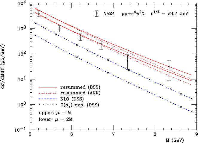
Figure 1: Comparison of the NLO (dashed) and resummed (solid (DSS) and dash-dotted (AKK)) calculations to the NA24 data [9], for two different choices of the renormalization and factorization scales, μ=M𝜇𝑀\mu=M (upper lines) and μ=2M𝜇2𝑀\mu=2M (lower lines). The crosses display the NLO 𝒪(αs)𝒪subscript𝛼𝑠{\cal O}(\alpha_{s}) expansion of the resummed cross section.
Refer to caption
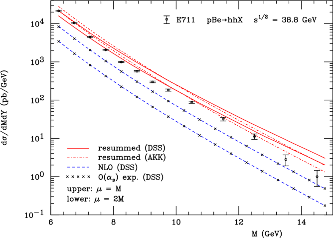
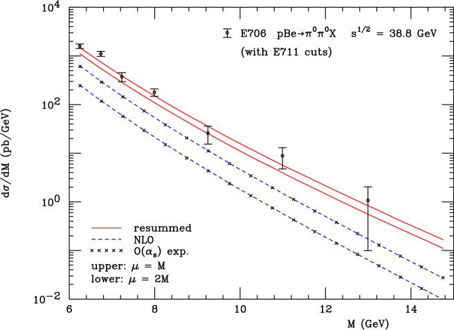
Figure 2: Same as Fig. 1, but for charged-hadron production for pp𝑝𝑝pp scattering at S=38.8𝑆38.8\sqrt{S}=38.8 GeV and with cuts appropriate for comparison to E711. The data are from [10].

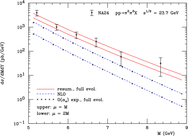
Figure 1 shows the comparison to the NA24 [9] data for ppπ0π0X𝑝𝑝superscript𝜋0superscript𝜋0𝑋pp\rightarrow\pi^{0}\pi^{0}X at S=23.7𝑆23.7\sqrt{S}=23.7 GeV. The cuts employed by NA24 are |cosθ|<0.4superscript𝜃0.4|\cos\theta^{*}|<0.4, average over |Y|<0.35𝑌0.35|Y|<0.35, and pTpair<1superscriptsubscript𝑝𝑇pair1p_{T}^{\mathrm{pair}}<1 GeV. We start by comparing the full NLO cross section to the first-order expansion of the resummed expression, that is, the last two terms in Eq. (48). This will help to gauge to what extent the soft-gluon terms constitute the dominant part of the cross section, so that their resummation is reliable. It turns out that the two terms agree to a remarkable degree. The dashed lines in Fig. 1 show the NLO cross section for scales 2M2𝑀2M (lower) and M𝑀M (upper), while the crosses give the NLO expansion of the resummed cross section. Their difference actually never exceeds 1%percent11\% for the kinematics relevant for NA24. The solid and dash-dotted lines in the figure present the full, and matched, resummed results for the DSS and AKK fragmentation sets, respectively, including “C𝐶C-coefficients” implemented as described in Sec. 3.2 (see Eq. (41)). One can see that resummation leads to a very significant enhancement of the theoretical prediction. A very good description of the NA24 data [9] is obtained for both sets, much better than for the NLO calculation which falls short of the data unless rather low renormalization and factorization scales are used. Also the scale dependence of the calculated cross section is much reduced by resummation. We note that the resummed result for the AKK set shows a somewhat steeper M𝑀M-dependence than that for the DSS set and lies lower at high M𝑀M. This may in part be due to the fact that large-N𝑁N resummation effects were included in the AKK analysis of the e+esuperscript𝑒superscript𝑒e^{+}e^{-} annihilation data, resulting probably in fragmentation functions that have an overall steeper z𝑧z-dependence. That said, given the still relatively large uncertainties of fragmentation functions overall, we also note that the different behavior of the AKK and DSS results might be just due to differing assumptions made in the respective analyses.

We next turn to the cross section for charged-hadron production, pBeh±h±X𝑝𝐵𝑒superscriptplus-or-minussuperscriptplus-or-minus𝑋pBe\rightarrow h^{\pm}h^{\pm}X, measured by E711 [10] at S=38.8𝑆38.8\sqrt{S}=38.8 GeV. We recall that we sum over the charges of the produced hadrons. The cuts applied by E711 were pT,i>2subscript𝑝𝑇𝑖2p_{T,i}>2 GeV, and average over 0.4<|Y|<0.20.4𝑌0.2-0.4<|Y|<0.2. The cut on the individual hadron transverse momenta is, in fact, irrelevant for the values of M𝑀M considered here. Furthermore, as stated in their Fig. 6 [10] for the pair mass distribution we apply pTpair<2superscriptsubscript𝑝𝑇pair2p_{T}^{\mathrm{pair}}<2 GeV, and 0.1<|cosθ|<0.250.1superscript𝜃0.250.1<|\cos\theta^{*}|<0.25. Figure 2 shows the data and our results. As before, the agreement between NLO and the NLO expansion of the resummed calculation is excellent. Again, resummation leads to an increase of the predicted cross section and a reduction of scale dependence. Even though the resummed results agree with the data much better than the NLO ones for the scales we have chosen, they tend to lie somewhat above the data, in particular at the highest values of M𝑀M. Keeping in mind the results for NA24, one may wonder if this might be in part related to the fragmentation functions for summed charged hadrons, which are probably slightly less well understood than those for pions, due to the contributions from the heavier kaons and, in particular, baryons. The trend for the resummed result to lie a bit high is, however, somewhat less pronounced for the AKK set which again produces results that are a bit steeper than the DSS ones.

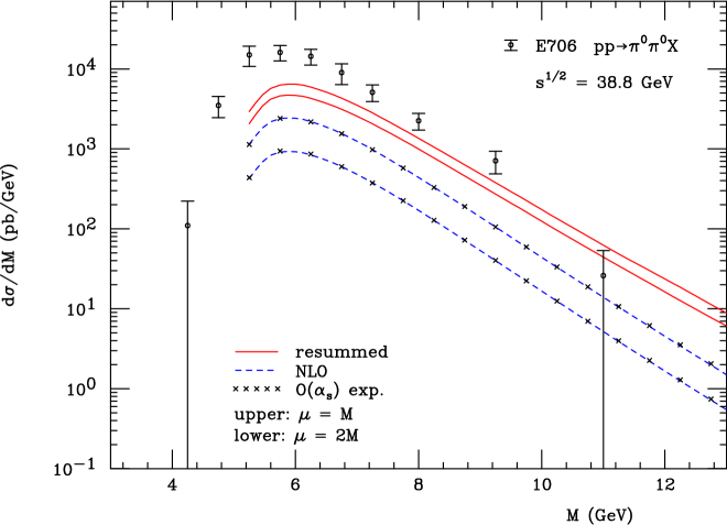
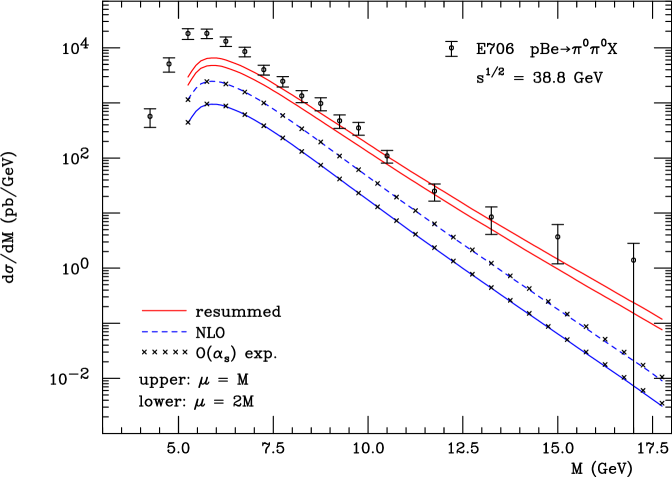
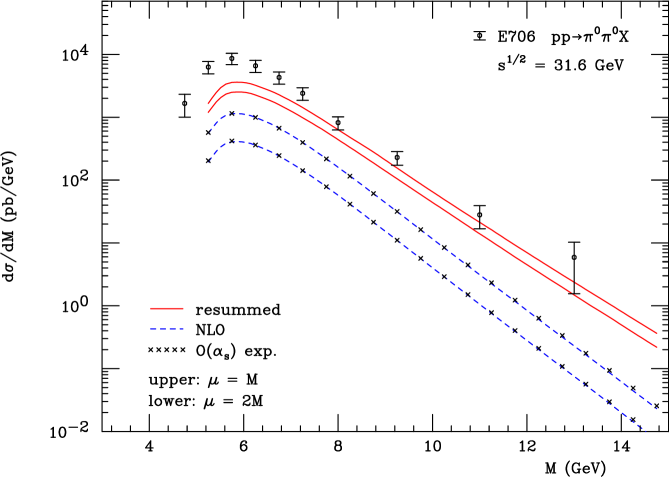
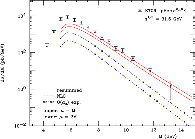
Figures 3 and 4 show the comparison of our results (for the DSS set) to the E706 data sets for neutral pion pair production in pp𝑝𝑝pp and pBe𝑝𝐵𝑒pBe scattering at S=38.8𝑆38.8\sqrt{S}=38.8 GeV (800 GeV beam energy), respectively. We do not take into account any nuclear effects for the Beryllium nucleus, except for the trivial isospin one. This has a very minor effect on the cross section, compared to pp𝑝𝑝pp. E706 used cuts fairly different from those applied in the data we have discussed so far. There were no explicit cuts on cosθsuperscript𝜃\cos\theta^{*}, pTpairsuperscriptsubscript𝑝𝑇pairp_{T}^{\mathrm{pair}} or Y𝑌Y, but instead cuts pT,i>pTcut=2.5subscript𝑝𝑇𝑖superscriptsubscript𝑝𝑇cut2.5p_{T,i}>p_{T}^{\mathrm{cut}}=2.5 GeV and either 1.05<ηi<0.551.05subscript𝜂𝑖0.55-1.05<\eta_{i}<0.55 (for the S=38.8𝑆38.8\sqrt{S}=38.8 GeV data) or 0.8<ηi<0.80.8subscript𝜂𝑖0.8-0.8<\eta_{i}<0.8 (for the S=31.6𝑆31.6\sqrt{S}=31.6 GeV data) on the transverse momenta and rapidities of the individual pions. The cut on transverse momentum, in particular, has a strong influence at the lower M𝑀M: in a rough approximation, it leads to a kinematic limit M2pT,i>5similar-to𝑀2subscript𝑝𝑇𝑖5M\sim 2p_{T,i}>5 GeV, so that the cross section has to decrease very rapidly once one decreases M𝑀M toward 5 GeV. This behavior is indeed seen in the figures.

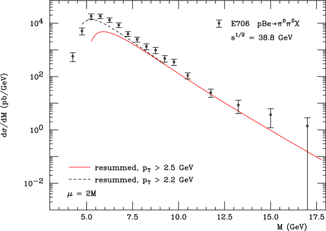
As in the previous cases, the NLO expansion of the resummed and the full NLO cross section agree extremely well, typically to better than 2%percent22\%. For the two scales we have chosen, the NLO cross sections fall well short of the data. It was noted in [14, 15] that in order for NLO to match the data, very low scales of μ=0.35M𝜇0.35𝑀\mu=0.35M have to be chosen. The resummed cross section, on the other hand, has much reduced scale dependence and describes the data very well for the more natural scales M𝑀M and 2M2𝑀2M, except at the lower M𝑀M where the cut pTcutsuperscriptsubscript𝑝𝑇cutp_{T}^{\mathrm{cut}} on the pT,isubscript𝑝𝑇𝑖p_{T,i} becomes relevant. One observes that the data extend to lower M𝑀M than the theoretical cross section, which basically cuts off at M=5𝑀5M=5 GeV as discussed above. A new scale becomes relevant here, the difference |M2pTcut|𝑀2superscriptsubscript𝑝𝑇cut|M-2p_{T}^{\mathrm{cut}}|. Higher order effects associated with this scale (which are different from the ones addressed by threshold resummation) and/or non-perturbative effects such as intrinsic transverse momenta [11] probably control the cross section here. It is also instructive to see that the cross section is very sensitive to the actual value of the cut on the pT,isubscript𝑝𝑇𝑖p_{T,i}. In Fig. 5 we show the resummed results for scale μ=2M𝜇2𝑀\mu=2M for pT,i>2.5subscript𝑝𝑇𝑖2.5p_{T,i}>2.5 GeV (as before) and pT,i>2.2subscript𝑝𝑇𝑖2.2p_{T,i}>2.2 GeV. One can see that with the lower cut the data are much better described. Experimental resolution effects might therefore have a significant influence on the comparison between data and theory here.

In order to check consistency, E706 also presented their pBe𝑝𝐵𝑒pBe data set at S=38.8𝑆38.8\sqrt{S}=38.8 GeV when the E711 cuts were applied instead of the E706 default ones. These data are found in [11]. Figure 6 shows the comparison for this case. One can see the same trends as before. Clearly, the description of the data by the resummed calculation is excellent. For this set of cuts, the cross section is not forced to turn down by kinematics at the lower M𝑀M, and theory and data agree well everywhere. Figures 7 and 8 show results corresponding to Figs. 34, but for the lower beam energy, 530 GeV, employed by E706 (S=31.6𝑆31.6\sqrt{S}=31.6 GeV).

Refer to caption
Figure 3: Comparison of the NLO (dashed) and resummed (solid) calculations (for the DSS fragmentation set) to the E706 pp𝑝𝑝pp data at S=38.8𝑆38.8\sqrt{S}=38.8 GeV [11], for two different choices of the renormalization and factorization scales, μ=M𝜇𝑀\mu=M (upper lines) and μ=2M𝜇2𝑀\mu=2M (lower lines). The crosses display the NLO 𝒪(αs)𝒪subscript𝛼𝑠{\cal O}(\alpha_{s}) expansion of the resummed cross section.
Refer to caption
Figure 4: Same as Fig. 3, but for proton-Beryllium scattering.
Refer to caption
Figure 5: Resummed cross section for scale μ=2M𝜇2𝑀\mu=2M and pT,i>2.2subscript𝑝𝑇𝑖2.2p_{T,i}>2.2 GeV (dashed), compared to the one with pT,i>2.5subscript𝑝𝑇𝑖2.5p_{T,i}>2.5 GeV shown previously in Fig. 4 (solid).
Refer to caption
Figure 6: Comparison to E706 data with a different set of cuts, corresponding to the ones applied by E711. The data with these cuts are from [11].
Refer to caption
Figure 7: Same as Fig. 3, but at S=31.6𝑆31.6\sqrt{S}=31.6 GeV.
Refer to caption
Figure 8: Same as Fig. 4, but at S=31.6𝑆31.6\sqrt{S}=31.6 GeV.

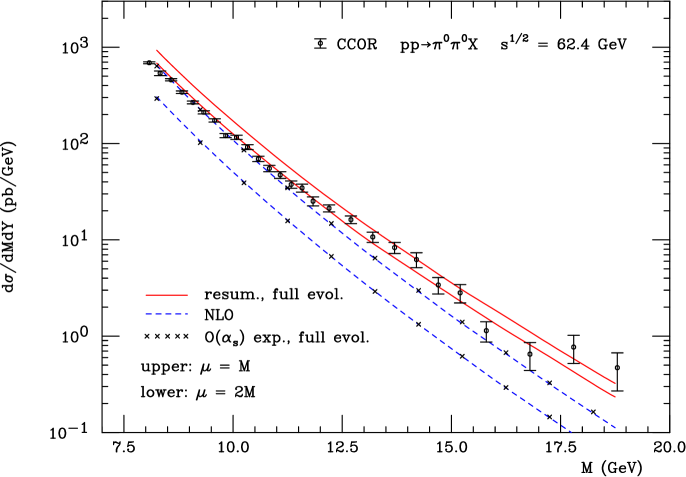
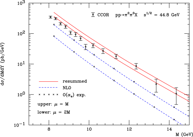
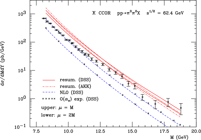
We finally turn to the data sets available at the highest energy, which are from the CCOR experiment at the ISR [12]. Two data set are available, at S=44.8𝑆44.8\sqrt{S}=44.8 GeV and 62.4 GeV. The cuts employed by CCOR were identical to those of NA24, |cosθ|<0.4superscript𝜃0.4|\cos\theta^{*}|<0.4, average over |Y|<0.35𝑌0.35|Y|<0.35, and pTpair<1superscriptsubscript𝑝𝑇pair1p_{T}^{\mathrm{pair}}<1 GeV. Figure 9 shows our results at S=44.8𝑆44.8\sqrt{S}=44.8 GeV. The resummed calculation again shows decreased scale dependence and describes the data much better than the NLO one. At the lower values of M𝑀M, it does show a tendency to lie above the data. Barring any issue with the data (which appear to have a certain unexpected “shoulder” around M=10𝑀10M=10 GeV or so), this might indicate that one gets too far from threshold for resummation to be very precise. On the other hand, the agreement between full NLO and the NLO expansion of the resummed cross section still remains very good, as can be seen from the figure. The trend for resummation to give results higher than the data becomes more pronounced at the higher energy, S=62.4𝑆62.4\sqrt{S}=62.4 GeV, as Fig. 10 shows, where we have used both the DSS and AKK sets of fragmentation functions. Although not easily seen from the figure, the NLO expansion of the resummed cross section starts to deviate more from the full NLO cross section than at the lower energies. At the lower M𝑀M shown, it can be higher by up to 7%percent77\%, which is still a relatively minor deviation, but could be indicative of the reason why the resummed result is high as well.

Clearly, any deviation between the full NLO cross section and the NLO expansion of the resummed one is due to terms that are formally suppressed by an inverse power of the Mellin moment N𝑁N near threshold. It is therefore interesting to explore the likely effects of such terms. This can be done by promoting the LO anomalous dimension in the evolution part in Eq. (42) from its diagonal form to the full one, as described in Sec. 3.2:

2Ai(1)lnN¯Bi(1)Pij(1),N,2superscriptsubscript𝐴𝑖1¯𝑁superscriptsubscript𝐵𝑖1superscriptsubscript𝑃𝑖𝑗1𝑁-2A_{i}^{(1)}\ln\bar{N}-B_{i}^{(1)}\rightarrow P_{ij}^{(1),N}\;, (52)

which includes the subleading terms in 1/N1𝑁1/N and full singlet mixing. For simplicity, we perform this modification only for the lowest order part of evolution, as indicated in Eqs. (43) and (52). The results obtained in this way are shown in Fig. 11. One can see that the resummed result obtained in this way indeed decreases significantly with respect to the one in Fig. 10 which was based on the diagonal evolution only, and is much closer to the data. At the same time, the agreement between the NLO cross section and the 𝒪(αs)𝒪subscript𝛼𝑠{\cal O}(\alpha_{s}) expanded resummed result becomes as good as what we encountered in the fixed-target case. Figure 12 presents the corresponding result for the case of NA24. Comparison with Fig. 1 shows that the effect of the subleading terms is much smaller here, as expected from the fact that one is closer to threshold in the case of NA24. Nonetheless, the effects lead to a slight further improvement between the resummed calculation and the data. In particular, they give the theoretical result a somewhat flatter behavior, which follows the trend of the data more closely overall. While the implementation of subleading terms in this way will require further study, this appears to be a promising approach for extending the applicability of threshold resummation into regimes where one is relatively far away from threshold.
Refer to caption
Figure 9: Comparison of the NLO (dashed) and resummed (solid) calculations to the CCOR data [9] at S=44.8𝑆44.8\sqrt{S}=44.8 GeV, for two different choices of the renormalization and factorization scales, μ=M𝜇𝑀\mu=M (upper lines) and μ=2M𝜇2𝑀\mu=2M (lower lines). The crosses display the NLO 𝒪(αs)𝒪subscript𝛼𝑠{\cal O}(\alpha_{s}) expansion of the resummed cross section.
Refer to caption
Figure 10: Same as Fig. 9, but for S=62.4𝑆62.4\sqrt{S}=62.4 GeV. We also show the resummed result obtained for the AKK set of fragmentation functions.
Refer to caption
Figure 11: As Fig. 10, but extending the diagonal evolution in the resummed formula to included subleading terms and singlet mixing, as shown in Eq. (52). We use the DSS set of fragmentation functions.
Refer to caption
Figure 12: Same as Fig. 11, but for the case of NA24.

That said, we remind the reader that already in the part that is leading near threshold we have made the approximation in Eq. (41) for our “C𝐶C-coefficients”. This, too, will need to be improved in the future, by taking into account the full color structure of the hard scattering function beyond LO, as we discussed in Sec. 3.2. To give a somewhat extreme example of the effects generated by the C𝐶C-coefficients, we have re-computed the resummed cross section for the case of CCOR at S=62.4𝑆62.4\sqrt{S}=62.4 GeV, but leaving out all effects of the the coefficients beyond NLO. In other words, we leave out the C𝐶C-coefficients in the first two terms on the right-hand-side of Eq. (48), keeping them of course in dσNLO𝑑superscript𝜎NLOd\sigma^{\mathrm{NLO}}. This is likely not a good approximation of the beyond-NLO hard coefficients, because the Cabcd(1)subscriptsuperscript𝐶1𝑎𝑏𝑐𝑑C^{(1)}_{ab\rightarrow cd} have π2superscript𝜋2\pi^{2} terms and logarithms in the renormalization scale μ𝜇\mu that are independent of the color channel and truly enter in the form given in Eq. (41). Some of these are in fact even known to exponentiate [17, 20, 21, 31, 40]. In any case, the result of this exercise is shown in Fig. 13, where it is also compared to our earlier calculation that included the C𝐶C-coefficients in the way discussed in Sec. 3.2. One can see that there is a sizable numerical difference, and that the scale dependence of the resummed result without the beyond-NLO C𝐶C-coefficients becomes significantly worse.

We finally turn to the distribution in cosθsuperscript𝜃\cos\theta^{*}, defined in Eq. (49), for which most of the experiments mentioned above have presented data as well. In fact, the CCOR data [12] for this observable were instrumental in establishing the QCD hard-scattering nature of pp𝑝𝑝pp interactions [41]. From the point of view of threshold resummation, the distribution in cosθsuperscript𝜃\cos\theta^{*} may appear somewhat less interesting than the pair mass one, since the threshold logarithms arise in 1τ^=1m^2/s^1^𝜏1superscript^𝑚2^𝑠1-\hat{\tau}=1-\hat{m}^{2}/\hat{s}, regardless of cosθsuperscript𝜃\cos\theta^{*}. In addition, the cosθsuperscript𝜃\cos\theta^{*} distributions are presented as normalized distributions of the form

dσ/dcosθdσ/dcosθ|cosθ=0,𝑑𝜎𝑑superscript𝜃evaluated-at𝑑𝜎𝑑superscript𝜃superscript𝜃0\frac{d\sigma/d\cos\theta^{*}}{d\sigma/d\cos\theta^{*}|_{\cos\theta^{*}=0}}\;, (53)

so that the main enhancement generated by threshold resummation is expected to cancel. Nonetheless, as we have seen in Sec. 3.2, the resummed expressions do contain additional dependence on ΔηΔ𝜂\Delta\eta beyond that present in the Born cross sections, which will affect the cosθsuperscript𝜃\cos\theta^{*} distribution at higher orders. This is visible from the soft part in Eq. (46) and also from the “C𝐶C-coefficients” in Eq. (41). Rather than going through an exhaustive comparison to all the available data, we just consider one example that is representative of the effects of threshold resummation on the cosθsuperscript𝜃\cos\theta^{*} distribution. Figure 14 shows the normalized distribution for the E711 case, where we have again summed over all charge states of the produced hadrons. The dashed lines show the NLO result calculated again with the code of [14], for scales μ=2M𝜇2𝑀\mu=2M and μ=M𝜇𝑀\mu=M. One can see that for these scales the NLO calculation is lower than the data for higher values of cosθsuperscript𝜃\cos\theta^{*}. The dot-dashed lines in Fig. 14 show the resummed results for scales μ=2M𝜇2𝑀\mu=2M and μ=M𝜇𝑀\mu=M. These show a steeper rise with cosθsuperscript𝜃\cos\theta^{*} and describe the data better than NLO for the scales shown. However, they still tend to lie below the data at higher values of cosθsuperscript𝜃\cos\theta^{*}. As was suggested in [12, 14, 15], for the cosθsuperscript𝜃\cos\theta^{*} distribution the hard scale in the partonic process will itself be a function of cosθsuperscript𝜃\cos\theta^{*}, so that it is more natural to choose a factorization/renormalization scale that reflects this feature. We therefore present our resummed results also for scales μ=2M𝜇2superscript𝑀\mu=2M^{*} and μ=M𝜇superscript𝑀\mu=M^{*}, where M=2M2(1cosθ)M^{*}{}^{2}=M^{2}(1-\cos\theta^{*}) which is proportional to the Mandelstam variable t^^𝑡\hat{t} in the partonic process. One observes that with these scale choices a very good description of the data is achieved. We note that in the NLO calculations presented in Refs. [14, 15] the scale was chosen proportional to the (average) transverse momenta of the produced hadrons, which for given M𝑀M also depend on cosθsuperscript𝜃\cos\theta^{*}. This resulted in a satisfactory description of the data, when scales effectively a factor two smaller than our Msuperscript𝑀M^{*} were used. Overall, the trend for the resummed cosθsuperscript𝜃\cos\theta^{*} distribution to lie higher than NLO and be in better agreement with the data is found to be a generic feature that occurs as well for the cases of the other experiments.
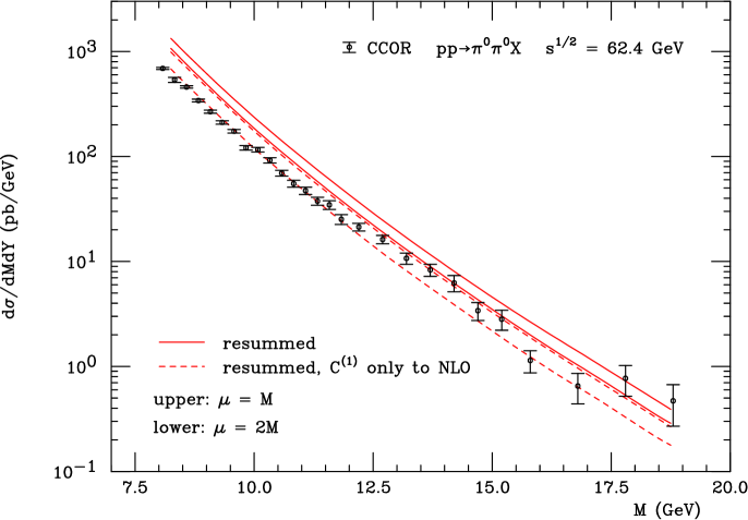
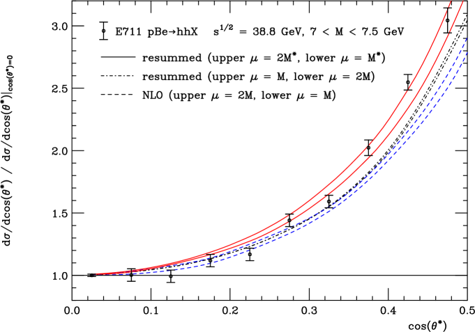
Refer to caption
Figure 13: Resummed results for the case of CCOR at S=62.4𝑆62.4\sqrt{S}=62.4 GeV. The solid lines show the results for scales M𝑀M and 2M2𝑀2M shown previously in Fig. 10, while the dashed ones were obtained by neglecting the contributions by the Cabcd(1)subscriptsuperscript𝐶1𝑎𝑏𝑐𝑑C^{(1)}_{ab\rightarrow cd} coefficients beyond NLO.
Refer to caption
Figure 14: Normalized distribution in cosθsuperscript𝜃\cos\theta^{*} (see (53)) for the case of charged-hadron production at E711. Dashed is NLO, while the dot-dashed and solid lines show resummed results. For the latter we have also used the scales μ=M𝜇superscript𝑀\mu=M^{*} and μ=2M𝜇2superscript𝑀\mu=2M^{*}, where M=2M2(1cosθ)M^{*}{}^{2}=M^{2}(1-\cos\theta^{*}).

5 Conclusions

We have investigated the effects of next-to-leading logarithmic threshold resummation on the cross section for di-hadron production in hadronic collisions, H1H2h1h2Xsubscript𝐻1subscript𝐻2subscript1subscript2𝑋H_{1}H_{2}\rightarrow h_{1}h_{2}X, for a range of invariant masses of the produced hadron pair. We have developed techniques to implement the resummation formalism at fixed rapidities for the produced hadrons and for all relevant experimental cuts. Extensions of these techniques to the level of next-to-next-lo-leading logarithms should be relatively straightforward in light of the close relation between the one- and two-loop soft anomalous dimension matrices [42].

For the fixed target and collider data studied here, the one-loop expansions of our resummed expressions approximate the corresponding exact one-loop cross sections excellently, to the level of a few percent and often less. In addition, with scales chosen to match the underlying hard scattering, the matched resummed cross sections typically explain the available data better than do NLO expressions at similar scales, with significantly reduced scale dependence.

An important extension of these methods will be in the production and fragmentation of heavy quarks and in jet cross sections, where similar resummation methods are applicable. Given the reduction in scale dependence, this could provide an improved control over Standard Model tests and backgrounds in new physics searches.

Acknowledgments

We are grateful to M. Begel and H.B. White for very helpful communications on the E706 and E711 data, respectively, and to S. Albino, B. Jäger, A. Mitov, M. Stratmann and M. Tannenbaum for useful discussions. We also thank J.F. Owens for providing his NLO code for di-hadron production, and for comments. W.V. is grateful to the U.S. Department of Energy (contract number DE-AC02-98CH10886) for providing the facilities essential for the completion of his work. This work was supported in part by the National Science Foundation, grants PHY-0354776, PHY-0354822 and PHY-0653342.

Appendix A

In this appendix we present some details for the calculation of the NLO partonic cross-sections near threshold. The virtual corrections have the 22222\rightarrow 2 kinematics of the Born terms and therefore fully contribute. They are proportional to δ(1τ^)𝛿1^𝜏\delta(1-\hat{\tau}). The real-emission 23232\rightarrow 3 contributions require more effort. We consider the reaction a(p1)+b(p2)c(k1)+d(k2)+e(k3)𝑎subscript𝑝1𝑏subscript𝑝2𝑐subscript𝑘1𝑑subscript𝑘2𝑒subscript𝑘3a(p_{1})+b(p_{2})\rightarrow c(k_{1})+d(k_{2})+e(k_{3}), where partons d𝑑d and e𝑒e fragment into the observed pair of hadrons and have pair mass m^2superscript^𝑚2\hat{m}^{2}. It is convenient to work in the c.m.s. of the observed outgoing hadrons. We can then write the three-body phase space in 42ε42𝜀4-2\varepsilon dimensions as

Φ3subscriptΦ3\displaystyle\Phi_{3} =\displaystyle= s(4π)4Γ(12ε)(4πs)2ε01𝑑τ^τ^ε(1τ^)12ε0𝑑ρρε(1+ρ)2+2ε𝑠superscript4𝜋4Γ12𝜀superscript4𝜋𝑠2𝜀superscriptsubscript01differential-d^𝜏superscript^𝜏𝜀superscript1^𝜏12𝜀superscriptsubscript0differential-d𝜌superscript𝜌𝜀superscript1𝜌22𝜀\displaystyle\frac{s}{(4\pi)^{4}\Gamma(1-2\varepsilon)}\left(\frac{4\pi}{s}\right)^{2\varepsilon}\,\int_{0}^{1}d\hat{\tau}\hat{\tau}^{-\varepsilon}(1-\hat{\tau})^{1-2\varepsilon}\int_{0}^{\infty}d\rho\rho^{-\varepsilon}(1+\rho)^{-2+2\varepsilon} (54)
×0πdψsin12εψ0πdθsin2εθ.\displaystyle\times\int_{0}^{\pi}d\psi\sin^{1-2\varepsilon}\psi\int_{0}^{\pi}d\theta\,\sin^{-2\varepsilon}\theta\;.

Here we define

ρ=(p1k2)2/(p2k2)2=e2Δη.𝜌superscriptsubscript𝑝1subscript𝑘22superscriptsubscript𝑝2subscript𝑘22superscripte2Δ𝜂\rho=(p_{1}-k_{2})^{2}/(p_{2}-k_{2})^{2}={\mathrm{e}}^{-2\Delta\eta}\;. (55)

Near threshold, the integration variables are given in terms of the Mandelstam variables of the process as follows:

(p1+p2)2=s^,(k2+k3)2=m^2=τ^s^,formulae-sequencesuperscriptsubscript𝑝1subscript𝑝22^𝑠superscriptsubscript𝑘2subscript𝑘32superscript^𝑚2^𝜏^𝑠\displaystyle(p_{1}+p_{2})^{2}=\hat{s}\;,\;\;\;(k_{2}+k_{3})^{2}=\hat{m}^{2}=\hat{\tau}\hat{s}\;,
(p1k1)2=s^(1τ^)2(1cosψ),(p2k1)2=s^(1τ^)2(1+cosψ),formulae-sequencesuperscriptsubscript𝑝1subscript𝑘12^𝑠1^𝜏21𝜓superscriptsubscript𝑝2subscript𝑘12^𝑠1^𝜏21𝜓\displaystyle(p_{1}-k_{1})^{2}=-\frac{\hat{s}(1-\hat{\tau})}{2}(1-\cos\psi)\;,\;\;\;(p_{2}-k_{1})^{2}=-\frac{\hat{s}(1-\hat{\tau})}{2}(1+\cos\psi)\;,
(p1k2)2=s^ρ1+ρ=(p2k3)2,(p2k2)2=s^1+ρ=(p1k3)2,formulae-sequencesuperscriptsubscript𝑝1subscript𝑘22^𝑠𝜌1𝜌superscriptsubscript𝑝2subscript𝑘32superscriptsubscript𝑝2subscript𝑘22^𝑠1𝜌superscriptsubscript𝑝1subscript𝑘32\displaystyle(p_{1}-k_{2})^{2}=-\frac{\hat{s}\rho}{1+\rho}=(p_{2}-k_{3})^{2}\;,\;\;\;(p_{2}-k_{2})^{2}=-\frac{\hat{s}}{1+\rho}=(p_{1}-k_{3})^{2}\;,
(k1+k2)2=s^(1τ^)2(1+sinψcosθ2ρ1+ρcosψ1ρ1+ρ),superscriptsubscript𝑘1subscript𝑘22^𝑠1^𝜏21𝜓𝜃2𝜌1𝜌𝜓1𝜌1𝜌\displaystyle(k_{1}+k_{2})^{2}=\frac{\hat{s}(1-\hat{\tau})}{2}\left(1+\sin\psi\cos\theta\,\frac{2\sqrt{\rho}}{1+\rho}-\cos\psi\,\frac{1-\rho}{1+\rho}\right)\;,
(k1+k3)2=s^(1τ^)2(1sinψcosθ2ρ1+ρ+cosψ1ρ1+ρ).superscriptsubscript𝑘1subscript𝑘32^𝑠1^𝜏21𝜓𝜃2𝜌1𝜌𝜓1𝜌1𝜌\displaystyle(k_{1}+k_{3})^{2}=\frac{\hat{s}(1-\hat{\tau})}{2}\left(1-\sin\psi\cos\theta\,\frac{2\sqrt{\rho}}{1+\rho}+\cos\psi\,\frac{1-\rho}{1+\rho}\right)\;. (56)

The phase space in Eq. (54) is used to integrate the squared 23232\rightarrow 3 matrix elements |abcde|2superscriptsubscript𝑎𝑏𝑐𝑑𝑒2|{\cal{M}}_{ab\rightarrow cde}|^{2}. For the latter one also assumes near-threshold kinematics. Since we want the partonic cross section at fixed τ^^𝜏\hat{\tau} and ΔηΔ𝜂\Delta\eta, we only need to perform the last two integrations in Eq. (54). The basic integral for these is [43]

0π𝑑ψ0π𝑑θsin12εψsin2εθ(1cosψ)j(1cosψcosχsinψcosθsinχ)ksuperscriptsubscript0𝜋differential-d𝜓superscriptsubscript0𝜋differential-d𝜃superscript12𝜀𝜓superscript2𝜀𝜃superscript1𝜓𝑗superscript1𝜓𝜒𝜓𝜃𝜒𝑘\displaystyle\int_{0}^{\pi}d\psi\int_{0}^{\pi}d\theta\,\frac{\sin^{1-2\varepsilon}\psi\sin^{-2\varepsilon}\theta}{(1-\cos\psi)^{j}(1-\cos\psi\cos\chi-\sin\psi\cos\theta\sin\chi)^{k}}
=2πΓ(12ε)Γ(1ε)2 2jkB(1εj,1εk)F12(j,k,1ε,cos2χ2),absent2𝜋Γ12𝜀Γsuperscript1𝜀2superscript2𝑗𝑘𝐵1𝜀𝑗1𝜀𝑘subscriptsubscript𝐹12𝑗𝑘1𝜀superscript2𝜒2\displaystyle\hskip 28.45274pt=2\pi\frac{\Gamma(1-2\varepsilon)}{\Gamma(1-\varepsilon)^{2}}\,2^{-j-k}\,B(1-\varepsilon-j,1-\varepsilon-k)\,{}_{2}F_{1}\left(j,k,1-\varepsilon,\cos^{2}\frac{\chi}{2}\right)\;, (57)

where F12subscriptsubscript𝐹12{}_{2}F_{1} is the Hypergeometric function. After integration over phase space and addition of the virtual corrections, infrared singularities cancel and only collinear singularities remain. These are removed by mass factorization, which we do in the MS¯¯MS{\overline{\rm MS}} scheme. Notice that since we are close to threshold only the diagonal splitting functions Pii(1)superscriptsubscript𝑃𝑖𝑖1P_{ii}^{(1)} contribute in this procedure. Combining all contributions, one arrives at the near-threshold structure of the partonic cross sections given in Eq. (17), for each subprocess that is already present at LO. The final step is to take Mellin moments in τ^^𝜏\hat{\tau} of the result, as described in Eq. (26). This gives for the partonic cross sections to NLO:

ω~abcdthr,LO+NLO(N,Δη,αs(μ),μ/m^)superscriptsubscript~𝜔𝑎𝑏𝑐𝑑thrLONLO𝑁Δ𝜂subscript𝛼𝑠𝜇𝜇^𝑚\displaystyle\tilde{\omega}_{ab\rightarrow cd}^{\mathrm{thr,LO+NLO}}\left(N,\Delta\eta,\alpha_{s}(\mu),\mu/\hat{m}\right) =\displaystyle= ωabcd(0)(Δη)superscriptsubscript𝜔𝑎𝑏𝑐𝑑0Δ𝜂\displaystyle\omega_{ab\rightarrow cd}^{(0)}(\Delta\eta) (58)
+αs(μ)π[ωabcd(1,0)(Δη,μ/m^)lnN¯ωabcd(1,1)(Δη,μ/m^)+12(ln2N¯+ζ(2))ωabcd(1,2)(Δη)],subscript𝛼𝑠𝜇𝜋delimited-[]subscriptsuperscript𝜔10𝑎𝑏𝑐𝑑Δ𝜂𝜇^𝑚¯𝑁subscriptsuperscript𝜔11𝑎𝑏𝑐𝑑Δ𝜂𝜇^𝑚12superscript2¯𝑁𝜁2subscriptsuperscript𝜔12𝑎𝑏𝑐𝑑Δ𝜂\displaystyle+\frac{\alpha_{s}(\mu)}{\pi}\left[\omega^{(1,0)}_{ab\rightarrow cd}(\Delta\eta,\mu/\hat{m})\,-\,\ln\bar{N}\;\omega^{(1,1)}_{ab\rightarrow cd}(\Delta\eta,\mu/\hat{m})+\frac{1}{2}\left(\ln^{2}\bar{N}+\zeta(2)\right)\;\omega^{(1,2)}_{ab\rightarrow cd}(\Delta\eta)\right]\;,

where terms subleading in N𝑁N have been neglected. The “C𝐶C-coefficients” defined in Eq. (41) are obtained from this as

Cabcd(1)(Δη,μ/m^)=ωabcd(1,0)(Δη,μ/m^)+12ζ(2)ωabcd(1,2)(Δη)ωabcd(0)(Δη).subscriptsuperscript𝐶1𝑎𝑏𝑐𝑑Δ𝜂𝜇^𝑚subscriptsuperscript𝜔10𝑎𝑏𝑐𝑑Δ𝜂𝜇^𝑚12𝜁2subscriptsuperscript𝜔12𝑎𝑏𝑐𝑑Δ𝜂superscriptsubscript𝜔𝑎𝑏𝑐𝑑0Δ𝜂C^{(1)}_{ab\rightarrow cd}\left(\Delta\eta,\mu/\hat{m}\right)=\frac{\omega^{(1,0)}_{ab\rightarrow cd}(\Delta\eta,\mu/\hat{m})+\frac{1}{2}\zeta(2)\,\omega^{(1,2)}_{ab\rightarrow cd}(\Delta\eta)}{\omega_{ab\rightarrow cd}^{(0)}(\Delta\eta)}\;. (59)

Appendix B

In this section we give the coefficients Cabcd(1)subscriptsuperscript𝐶1𝑎𝑏𝑐𝑑C^{(1)}_{ab\rightarrow cd} for each subprocess contributing to the production of our di-hadron final state, resulting from the calculation outlined in Appendix A. In all expressions below, μ𝜇\mu is the renormalization scale. The dependence on the factorization scale is already included in the function isubscript𝑖{\cal E}_{i} in Eq. (43). As before, we define ρe2Δη𝜌superscripte2Δ𝜂\rho\equiv{\mathrm{e}}^{-2\Delta\eta}.

qqqq𝑞superscript𝑞𝑞superscript𝑞qq^{\prime}\rightarrow qq^{\prime}:
We define:

Qqq1+(1+ρ)2.subscript𝑄𝑞superscript𝑞1superscript1𝜌2Q_{qq^{\prime}}\equiv 1+(1+\rho)^{2}\;. (60)

We then have:

Cqqqq(1)(Δη,μ/m^)superscriptsubscript𝐶𝑞superscript𝑞𝑞superscript𝑞1Δ𝜂𝜇^𝑚\displaystyle C_{qq^{\prime}\rightarrow qq^{\prime}}^{(1)}\left(\Delta\eta,\mu/\hat{m}\right) =\displaystyle= 2πb0lnμ2m^2+(56Qqq+1312)ln2ρ+(5613Qqq)ln2(1+ρ)2𝜋subscript𝑏0superscript𝜇2superscript^𝑚256subscript𝑄𝑞superscript𝑞1312superscript2𝜌5613subscript𝑄𝑞superscript𝑞superscript21𝜌\displaystyle 2\pi b_{0}\ln\frac{\mu^{2}}{\hat{m}^{2}}+\left(\frac{5}{6Q_{qq^{\prime}}}+\frac{13}{12}\right)\ln^{2}\rho+\left(\frac{5}{6}-\frac{1}{3Q_{qq^{\prime}}}\right)\ln^{2}(1+\rho) (61)
+(83+14+9ρ6Qqq)lnρ+(43+23Qqq)ln(1+ρ)lnρ83149𝜌6subscript𝑄𝑞superscript𝑞𝜌4323subscript𝑄𝑞superscript𝑞1𝜌𝜌\displaystyle+\left(-\frac{8}{3}+\frac{14+9\rho}{6Q_{qq^{\prime}}}\right)\ln\rho+\left(-\frac{4}{3}+\frac{2}{3Q_{qq^{\prime}}}\right)\ln(1+\rho)\ln\rho
ρ3Qqqln(1+ρ)+7π26Qqq+Nf3lnρ1+ρ5Nf9𝜌3subscript𝑄𝑞superscript𝑞1𝜌7superscript𝜋26subscript𝑄𝑞superscript𝑞subscript𝑁𝑓3𝜌1𝜌5subscript𝑁𝑓9\displaystyle-\frac{\rho}{3Q_{qq^{\prime}}}\ln(1+\rho)+\frac{7\pi^{2}}{6Q_{qq^{\prime}}}+\frac{N_{f}}{3}\ln\frac{\rho}{1+\rho}-\frac{5N_{f}}{9}
+83Li2(ρ1+ρ)+32ln(1+ρ)+47π236+72.83subscriptLi2𝜌1𝜌321𝜌47superscript𝜋23672\displaystyle+\frac{8}{3}\text{Li}_{2}\left(\frac{\rho}{1+\rho}\right)+\frac{3}{2}\ln(1+\rho)+\frac{47\pi^{2}}{36}+\frac{7}{2}\;.

qq¯qq¯𝑞superscript¯𝑞𝑞superscript¯𝑞q\bar{q}^{\prime}\rightarrow q\bar{q}^{\prime}:
We have:

Cqq¯qq¯(1)(Δη,μ/m^)superscriptsubscript𝐶𝑞superscript¯𝑞𝑞superscript¯𝑞1Δ𝜂𝜇^𝑚\displaystyle C_{q\bar{q}^{\prime}\rightarrow q\bar{q}^{\prime}}^{(1)}\left(\Delta\eta,\mu/\hat{m}\right) =\displaystyle= Cqqqq(1)(Δη,μ/m^)+56{(12Qqq)[(1+lnρ)lnρ+π22]\displaystyle C_{qq^{\prime}\rightarrow qq^{\prime}}^{(1)}\left(\Delta\eta,\mu/\hat{m}\right)+\frac{5}{6}\left\{\left(1-\frac{2}{Q_{qq^{\prime}}}\right)\left[(1+\ln\rho)\ln\rho+\frac{\pi^{2}}{2}\right]\right. (62)
ρQqqln(1+ρ)+(321Qqq)ln(1+ρ)ln1+ρρ22Li2(ρ1+ρ)}.\displaystyle\left.-\frac{\rho}{Q_{qq^{\prime}}}\ln(1+\rho)+\left(\frac{3}{2}-\frac{1}{Q_{qq^{\prime}}}\right)\ln(1+\rho)\ln\frac{1+\rho}{\rho^{2}}-2\text{Li}_{2}\left(\frac{\rho}{1+\rho}\right)\right\}\;.

qqqq𝑞𝑞𝑞𝑞qq\rightarrow qq:
We define:

Qqq(1ρ+ρ2)(3+5ρ+3ρ2)(1+ρ(1+ρ)).subscript𝑄𝑞𝑞1𝜌superscript𝜌235𝜌3superscript𝜌21𝜌1𝜌Q_{qq}\equiv\frac{(1-\rho+\rho^{2})(3+5\rho+3\rho^{2})}{(1+\rho(1+\rho))}\;. (63)

We then have:

Cqqqq(1)(Δη,μ/m^)superscriptsubscript𝐶𝑞𝑞𝑞𝑞1Δ𝜂𝜇^𝑚\displaystyle C_{qq\rightarrow qq}^{(1)}\left(\Delta\eta,\mu/\hat{m}\right) =\displaystyle= 2πb0lnμ2m^2+8Qqq(1ρ2)Li2(ρ1+ρ)2𝜋subscript𝑏0superscript𝜇2superscript^𝑚28subscript𝑄𝑞𝑞1superscript𝜌2subscriptLi2𝜌1𝜌\displaystyle 2\pi b_{0}\ln\frac{\mu^{2}}{\hat{m}^{2}}+\frac{8}{Q_{qq}}\left(1-\rho^{2}\right)\text{Li}_{2}\left(\frac{\rho}{1+\rho}\right) (64)
+(7659ρ48Qqq+54Qqqρ+416(3+5ρ+3ρ2))ln2ρ7659𝜌48subscript𝑄𝑞𝑞54subscript𝑄𝑞𝑞𝜌41635𝜌3superscript𝜌2superscript2𝜌\displaystyle+\left(\frac{7}{6}-\frac{59\rho}{48Q_{qq}}+\frac{5}{4\ Q_{qq}}-\frac{\rho+4}{16\left(3+5\rho+3\rho^{2}\right)}\right)\ln^{2}\rho
(12ρ2+3ρ4)2Qqqln2(1+ρ)+lnρ12Qqq(37ρ71+(178ρ)Qqq3+5ρ+3ρ2)12superscript𝜌23𝜌42subscript𝑄𝑞𝑞superscript21𝜌𝜌12subscript𝑄𝑞𝑞37𝜌71178𝜌subscript𝑄𝑞𝑞35𝜌3superscript𝜌2\displaystyle-\frac{\left(12\rho^{2}+3\rho-4\right)}{2Q_{qq}}\ln^{2}(1+\rho)+\frac{\ln\rho}{12Q_{qq}}\left(37\rho-71+\frac{(17-8\rho)\,Q_{qq}}{3+5\rho+3\rho^{2}}\right)
+(7374Qqq(65ρ)53ρ612(3+5ρ+3ρ2))ln(1+ρ)lnρ7374subscript𝑄𝑞𝑞65𝜌53𝜌61235𝜌3superscript𝜌21𝜌𝜌\displaystyle+\left(\frac{7}{3}-\frac{7}{4Q_{qq}}\left(6-5\rho\right)-\frac{53\rho-6}{12\left(3+5\rho+3\rho^{2}\right)}\right)\ln(1+\rho)\ln\rho
+(32ρ4Qqqρ4(3+5ρ+3ρ2))ln(1+ρ)32𝜌4subscript𝑄𝑞𝑞𝜌435𝜌3superscript𝜌21𝜌\displaystyle+\left(\frac{3}{2}-\frac{\rho}{4Q_{qq}}-\frac{\rho}{4\left(3+5\rho+3\rho^{2}\right)}\right)\ln(1+\rho)
+Nf(2ρ2Qqq+ρ3(3+5ρ+3ρ2))lnρ13Nfln(1+ρ)5Nf9subscript𝑁𝑓2𝜌2subscript𝑄𝑞𝑞𝜌335𝜌3superscript𝜌2𝜌13subscript𝑁𝑓1𝜌5subscript𝑁𝑓9\displaystyle+N_{f}\left(\frac{2-\rho}{2Q_{qq}}+\frac{\rho}{3\left(3+5\rho+3\rho^{2}\right)}\right)\ln\rho-\frac{1}{3}N_{f}\ln(1+\rho)-\frac{5N_{f}}{9}
+72(1+23π2)π23Qqq(4+4116ρ)71π2ρ144(3+5ρ+3ρ2).72123superscript𝜋2superscript𝜋23subscript𝑄𝑞𝑞44116𝜌71superscript𝜋2𝜌14435𝜌3superscript𝜌2\displaystyle+\frac{7}{2}\left(1+\frac{2}{3}\pi^{2}\right)-\frac{\pi^{2}}{3Q_{qq}}\left(4+\frac{41}{16}\rho\right)-\frac{71\pi^{2}\rho}{144\left(3+5\rho+3\rho^{2}\right)}\;.

qq¯qq¯𝑞¯𝑞superscript𝑞superscript¯𝑞q\bar{q}\rightarrow q^{\prime}\bar{q}^{\prime}:
We define:

Qqq¯1+ρ2.subscript𝑄superscript𝑞superscript¯𝑞1superscript𝜌2Q_{q^{\prime}\bar{q}^{\prime}}\equiv 1+\rho^{2}\;. (65)

We then have:

Cqq¯qq¯(1)(Δη,μ/m^)superscriptsubscript𝐶𝑞¯𝑞superscript𝑞superscript¯𝑞1Δ𝜂𝜇^𝑚\displaystyle C_{q\bar{q}\rightarrow q^{\prime}\bar{q}^{\prime}}^{(1)}\left(\Delta\eta,\mu/\hat{m}\right) =\displaystyle= 2πb0lnμ2m^2+74(123Qqq¯)ln2ρ512(1+2Qqq¯)ln2(1+ρ)2𝜋subscript𝑏0superscript𝜇2superscript^𝑚274123subscript𝑄superscript𝑞superscript¯𝑞superscript2𝜌51212subscript𝑄superscript𝑞superscript¯𝑞superscript21𝜌\displaystyle 2\pi b_{0}\ln\frac{\mu^{2}}{\hat{m}^{2}}+\frac{7}{4}\left(1-\frac{2}{3Q_{q^{\prime}\bar{q}^{\prime}}}\right)\ln^{2}\rho-\frac{5}{12}\left(1+\frac{2}{Q_{q^{\prime}\bar{q}^{\prime}}}\right)\ln^{2}(1+\rho) (66)
+7(1+ρ)6Qqq¯lnρ76(12Qqq¯)ln(1+ρ)lnρ13(1+5+9ρ2Qqq¯)ln(1+ρ)71𝜌6subscript𝑄superscript𝑞superscript¯𝑞𝜌7612subscript𝑄superscript𝑞superscript¯𝑞1𝜌𝜌13159𝜌2subscript𝑄superscript𝑞superscript¯𝑞1𝜌\displaystyle+\frac{7(1+\rho)}{6Q_{q^{\prime}\bar{q}^{\prime}}}\ln\rho-\frac{7}{6}\left(1-\frac{2}{Q_{q^{\prime}\bar{q}^{\prime}}}\right)\ln(1+\rho)\ln\rho-\frac{1}{3}\left(1+\frac{5+9\rho}{2Q_{q^{\prime}\bar{q}^{\prime}}}\right)\ln(1+\rho)
5Nf953Li2(ρ1+ρ)+16(21+4π2).5subscript𝑁𝑓953subscriptLi2𝜌1𝜌16214superscript𝜋2\displaystyle-\frac{5N_{f}}{9}-\frac{5}{3}\text{Li}_{2}\left(\frac{\rho}{1+\rho}\right)+\frac{1}{6}\left(21+4\pi^{2}\right)\;.

qq¯qq¯𝑞¯𝑞𝑞¯𝑞q\bar{q}\rightarrow q\bar{q}:
We define:

Qqq¯(1)3+ρ(1+ρ),subscriptsuperscript𝑄1𝑞¯𝑞3𝜌1𝜌\displaystyle Q^{(1)}_{q\bar{q}}\equiv 3+\rho(1+\rho)\;,
Qqq¯(2)1+3ρ(1+ρ).subscriptsuperscript𝑄2𝑞¯𝑞13𝜌1𝜌\displaystyle Q^{(2)}_{q\bar{q}}\equiv 1+3\rho(1+\rho)\;. (67)

We then have:

Cqq¯qq¯(1)(Δη,μ/m^)superscriptsubscript𝐶𝑞¯𝑞𝑞¯𝑞1Δ𝜂𝜇^𝑚\displaystyle C_{q\bar{q}\rightarrow q\bar{q}}^{(1)}\left(\Delta\eta,\mu/\hat{m}\right) =\displaystyle= 2πb0lnμ2m^2+Nf(16+(1+2ρ)(18Qqq¯(1)+18Qqq¯(2)))ln(ρ1+ρ)2𝜋subscript𝑏0superscript𝜇2superscript^𝑚2subscript𝑁𝑓1612𝜌18subscriptsuperscript𝑄1𝑞¯𝑞18subscriptsuperscript𝑄2𝑞¯𝑞𝜌1𝜌\displaystyle 2\pi b_{0}\ln\frac{\mu^{2}}{\hat{m}^{2}}+N_{f}\left(\frac{1}{6}+(1+2\rho)\left(\frac{1}{8Q^{(1)}_{q\bar{q}}}+\frac{1}{8Q^{(2)}_{q\bar{q}}}\right)\right)\ln\left(\frac{\rho}{1+\rho}\right) (68)
+Li2(ρ1+ρ)(5+4ρ2Qqq¯(1)+1+4ρ2Qqq¯(2)13)+π2(5(9+14ρ)96Qqq¯(1)+155+282ρ288Qqq¯(2)+4336)subscriptLi2𝜌1𝜌54𝜌2subscriptsuperscript𝑄1𝑞¯𝑞14𝜌2subscriptsuperscript𝑄2𝑞¯𝑞13superscript𝜋25914𝜌96subscriptsuperscript𝑄1𝑞¯𝑞155282𝜌288subscriptsuperscript𝑄2𝑞¯𝑞4336\displaystyle+\text{Li}_{2}\left(\frac{\rho}{1+\rho}\right)\left(\frac{5+4\rho}{2Q^{(1)}_{q\bar{q}}}+\frac{1+4\rho}{2Q^{(2)}_{q\bar{q}}}-\frac{1}{3}\right)+\pi^{2}\left(\frac{5(9+14\rho)}{96Q^{(1)}_{q\bar{q}}}+\frac{155+282\rho}{288Q^{(2)}_{q\bar{q}}}+\frac{43}{36}\right)
+(4ρ7964Qqq¯(1)+61+180ρ576Qqq¯(2)+6536)ln2ρ+(13+124ρ64Qqq¯(1)+361+972ρ576Qqq¯(2)+2936)ln2(1+ρ)4𝜌7964subscriptsuperscript𝑄1𝑞¯𝑞61180𝜌576subscriptsuperscript𝑄2𝑞¯𝑞6536superscript2𝜌13124𝜌64subscriptsuperscript𝑄1𝑞¯𝑞361972𝜌576subscriptsuperscript𝑄2𝑞¯𝑞2936superscript21𝜌\displaystyle+\left(\frac{4\rho-79}{64Q^{(1)}_{q\bar{q}}}+\frac{61+180\rho}{576Q^{(2)}_{q\bar{q}}}+\frac{65}{36}\right)\ln^{2}\rho+\left(\frac{13+124\rho}{64Q^{(1)}_{q\bar{q}}}+\frac{361+972\rho}{576Q^{(2)}_{q\bar{q}}}+\frac{29}{36}\right)\ln^{2}(1+\rho)
+(7ρ16Qqq¯(1)35+71ρ48Qqq¯(2)1112)lnρ+(6164ρ32Qqq¯(1)247+576ρ288Qqq¯(2)229)ln(1+ρ)lnρ7𝜌16subscriptsuperscript𝑄1𝑞¯𝑞3571𝜌48subscriptsuperscript𝑄2𝑞¯𝑞1112𝜌6164𝜌32subscriptsuperscript𝑄1𝑞¯𝑞247576𝜌288subscriptsuperscript𝑄2𝑞¯𝑞2291𝜌𝜌\displaystyle+\left(\frac{7-\rho}{16Q^{(1)}_{q\bar{q}}}-\frac{35+71\rho}{48Q^{(2)}_{q\bar{q}}}-\frac{11}{12}\right)\ln\rho+\left(\frac{61-64\rho}{32Q^{(1)}_{q\bar{q}}}-\frac{247+576\rho}{288Q^{(2)}_{q\bar{q}}}-\frac{22}{9}\right)\ln(1+\rho)\ln\rho
+(8+ρ16Qqq¯(1)+36+71ρ48Qqq¯(2)+712)ln(1+ρ)5Nf9+72.8𝜌16subscriptsuperscript𝑄1𝑞¯𝑞3671𝜌48subscriptsuperscript𝑄2𝑞¯𝑞7121𝜌5subscript𝑁𝑓972\displaystyle+\left(\frac{8+\rho}{16Q^{(1)}_{q\bar{q}}}+\frac{36+71\rho}{48Q^{(2)}_{q\bar{q}}}+\frac{7}{12}\right)\ln(1+\rho)-\frac{5N_{f}}{9}+\frac{7}{2}\;.

qq¯gg𝑞¯𝑞𝑔𝑔q\bar{q}\rightarrow gg:
We define:

Gqq¯(1+ρ2)(4ρ+4ρ2).subscript𝐺𝑞¯𝑞1superscript𝜌24𝜌4superscript𝜌2G_{q\bar{q}}\equiv(1+\rho^{2})(4-\rho+4\rho^{2})\;. (69)

We then have:

Cqq¯gg(1)(Δη,μ/m^)superscriptsubscript𝐶𝑞¯𝑞𝑔𝑔1Δ𝜂𝜇^𝑚\displaystyle C_{q\bar{q}\rightarrow gg}^{(1)}\left(\Delta\eta,\mu/\hat{m}\right) =\displaystyle= 2πb0lnμ2m^2272Gqq¯(1ρ4)Li2(ρ1+ρ)2𝜋subscript𝑏0superscript𝜇2superscript^𝑚2272subscript𝐺𝑞¯𝑞1superscript𝜌4subscriptLi2𝜌1𝜌\displaystyle 2\pi b_{0}\ln\frac{\mu^{2}}{\hat{m}^{2}}-\frac{27}{2G_{q\bar{q}}}\left(1-\rho^{4}\right)\text{Li}_{2}\left(\frac{\rho}{1+\rho}\right) (70)
+148(1+2ρGqq¯(133+13ρ)+124311ρ4ρ+4ρ2)ln2ρ14812𝜌subscript𝐺𝑞¯𝑞13313𝜌124311𝜌4𝜌4superscript𝜌2superscript2𝜌\displaystyle+\frac{1}{48}\left(1+\frac{2\rho}{G_{q\bar{q}}}\left(133+13\rho\right)+\frac{124-311\rho}{4-\rho+4\rho^{2}}\right)\ln^{2}\rho
+148(69+52ρ2Gqq¯ρ+6484ρ+4ρ2)ln2(1+ρ)1486952superscript𝜌2subscript𝐺𝑞¯𝑞𝜌6484𝜌4superscript𝜌2superscript21𝜌\displaystyle+\frac{1}{48}\left(69+\frac{52\rho^{2}}{G_{q\bar{q}}}-\frac{\rho+648}{4-\rho+4\rho^{2}}\right)\ln^{2}(1+\rho)
+16(ρGqq¯(3+89ρ)+48+5ρ4ρ+4ρ2)lnρ16𝜌subscript𝐺𝑞¯𝑞389𝜌485𝜌4𝜌4superscript𝜌2𝜌\displaystyle+\frac{1}{6}\left(-\frac{\rho}{G_{q\bar{q}}}\left(3+89\rho\right)+\frac{48+5\rho}{4-\rho+4\rho^{2}}\right)\ln\rho
+(89ρ23Gqq¯19ρ6(4ρ+4ρ2)2)ln(1+ρ)89superscript𝜌23subscript𝐺𝑞¯𝑞19𝜌64𝜌4superscript𝜌221𝜌\displaystyle+\left(\frac{89\rho^{2}}{3G_{q\bar{q}}}-\frac{19\rho}{6\left(4-\rho+4\rho^{2}\right)}-2\right)\ln(1+\rho)
+124(192ρGqq¯(133+13ρ)+200+149ρ4ρ+4ρ2)lnρln(1+ρ)124192𝜌subscript𝐺𝑞¯𝑞13313𝜌200149𝜌4𝜌4superscript𝜌2𝜌1𝜌\displaystyle+\frac{1}{24}\left(-19-\frac{2\rho}{G_{q\bar{q}}}\left(133+13\rho\right)+\frac{200+149\rho}{4-\rho+4\rho^{2}}\right)\ln\rho\ln(1+\rho)
154Gqq¯ρ(1ρ)2+9π2(4ρ)16(4ρ+4ρ2)+191π2144143.154subscript𝐺𝑞¯𝑞𝜌superscript1𝜌29superscript𝜋24𝜌164𝜌4superscript𝜌2191superscript𝜋2144143\displaystyle-\frac{15}{4G_{q\bar{q}}}\rho(1-\rho)^{2}+\frac{9\pi^{2}(4-\rho)}{16\left(4-\rho+4\rho^{2}\right)}+\frac{191\pi^{2}}{144}-\frac{14}{3}\;.

qgqg𝑞𝑔𝑞𝑔qg\rightarrow qg:
We define:

Qqg(1)2(1+ρ)+ρ2,subscriptsuperscript𝑄1𝑞𝑔21𝜌superscript𝜌2\displaystyle Q^{(1)}_{qg}\equiv 2(1+\rho)+\rho^{2}\;,
Qqg(2)9(1+ρ)+4ρ2.subscriptsuperscript𝑄2𝑞𝑔91𝜌4superscript𝜌2\displaystyle Q^{(2)}_{qg}\equiv 9(1+\rho)+4\rho^{2}\;. (71)

We then have:

Cqgqg(1)(Δη,μ/m^)superscriptsubscript𝐶𝑞𝑔𝑞𝑔1Δ𝜂𝜇^𝑚\displaystyle C_{qg\rightarrow qg}^{(1)}\left(\Delta\eta,\mu/\hat{m}\right) =\displaystyle= 2πb0lnμ2m^2143+15(1+ρ)(2+ρ)24Qqg(1)Qqg(2)2𝜋subscript𝑏0superscript𝜇2superscript^𝑚2143151𝜌superscript2𝜌24subscriptsuperscript𝑄1𝑞𝑔subscriptsuperscript𝑄2𝑞𝑔\displaystyle 2\pi b_{0}\ln\frac{\mu^{2}}{\hat{m}^{2}}-\frac{14}{3}+\frac{15(1+\rho)(2+\rho)^{2}}{4Q^{(1)}_{qg}Q^{(2)}_{qg}} (72)
+π2(146+13ρ24Qqg(1)3(109+13ρ)16Qqg(2)+241144)superscript𝜋214613𝜌24subscriptsuperscript𝑄1𝑞𝑔310913𝜌16subscriptsuperscript𝑄2𝑞𝑔241144\displaystyle+\pi^{2}\left(\frac{146+13\rho}{24Q^{(1)}_{qg}}-\frac{3(109+13\rho)}{16Q^{(2)}_{qg}}+\frac{241}{144}\right)
+((1+ρ)(1312Qqg(1)1516Qqg(2))+1716)ln2ρ+(1+ρ)(893Qqg(1)2312Qqg(2))lnρ1𝜌1312subscriptsuperscript𝑄1𝑞𝑔1516subscriptsuperscript𝑄2𝑞𝑔1716superscript2𝜌1𝜌893subscriptsuperscript𝑄1𝑞𝑔2312subscriptsuperscript𝑄2𝑞𝑔𝜌\displaystyle+\left((1+\rho)\left(\frac{13}{12Q^{(1)}_{qg}}-\frac{15}{16Q^{(2)}_{qg}}\right)+\frac{17}{16}\right)\ln^{2}\rho+(1+\rho)\left(\frac{89}{3Q^{(1)}_{qg}}-\frac{231}{2Q^{(2)}_{qg}}\right)\ln\rho
+(13ρ12024Qqg(1)+3(173+41ρ)16Qqg(2)2716)ln2(1+ρ)13𝜌12024subscriptsuperscript𝑄1𝑞𝑔317341𝜌16subscriptsuperscript𝑄2𝑞𝑔2716superscript21𝜌\displaystyle+\left(\frac{13\rho-120}{24Q^{(1)}_{qg}}+\frac{3(173+41\rho)}{16Q^{(2)}_{qg}}-\frac{27}{16}\right)\ln^{2}(1+\rho)
+(86+89ρ6Qqg(1)+3(43+39ρ)2Qqg(2)2)ln(1+ρ)+(3124+27(ρ3)8Qqg(2))Li2(ρ1+ρ)8689𝜌6subscriptsuperscript𝑄1𝑞𝑔34339𝜌2subscriptsuperscript𝑄2𝑞𝑔21𝜌312427𝜌38subscriptsuperscript𝑄2𝑞𝑔subscriptLi2𝜌1𝜌\displaystyle+\left(-\frac{86+89\rho}{6Q^{(1)}_{qg}}+\frac{3(43+39\rho)}{2Q^{(2)}_{qg}}-2\right)\ln(1+\rho)+\left(\frac{31}{24}+\frac{27(\rho-3)}{8Q^{(2)}_{qg}}\right)\text{Li}_{2}\left(\frac{\rho}{1+\rho}\right)
+(12013ρ12Qqg(1)3(155+23ρ)8Qqg(2)+3124)lnρln(1+ρ).12013𝜌12subscriptsuperscript𝑄1𝑞𝑔315523𝜌8subscriptsuperscript𝑄2𝑞𝑔3124𝜌1𝜌\displaystyle+\left(\frac{120-13\rho}{12Q^{(1)}_{qg}}-\frac{3(155+23\rho)}{8Q^{(2)}_{qg}}+\frac{31}{24}\right)\ln\rho\ln(1+\rho)\;.

ggqq¯𝑔𝑔𝑞¯𝑞gg\rightarrow q\bar{q}:
We have:

Cggqq¯(1)(Δη,μ/m^)superscriptsubscript𝐶𝑔𝑔𝑞¯𝑞1Δ𝜂𝜇^𝑚\displaystyle C_{gg\rightarrow q\bar{q}}^{(1)}\left(\Delta\eta,\mu/\hat{m}\right) =\displaystyle= Cqq¯gg(1)(Δη,μ/m^).superscriptsubscript𝐶𝑞¯𝑞𝑔𝑔1Δ𝜂𝜇^𝑚\displaystyle C_{q\bar{q}\rightarrow gg}^{(1)}\left(\Delta\eta,\mu/\hat{m}\right)\;. (73)

gggg𝑔𝑔𝑔𝑔gg\rightarrow gg:
We define:

Ggg1+ρ(1+ρ).subscript𝐺𝑔𝑔1𝜌1𝜌G_{gg}\equiv 1+\rho(1+\rho)\;. (74)

We then have:

Cgggg(1)(Δη,μ/m^)superscriptsubscript𝐶𝑔𝑔𝑔𝑔1Δ𝜂𝜇^𝑚\displaystyle C_{gg\rightarrow gg}^{(1)}\left(\Delta\eta,\mu/\hat{m}\right) =\displaystyle= 2πb0lnμ2m^2+Nf(59+3ρ2(1+ρ)28Ggg3+π2ρ(1+ρ2)(1+ρ)216Ggg3)2𝜋subscript𝑏0superscript𝜇2superscript^𝑚2subscript𝑁𝑓593superscript𝜌2superscript1𝜌28superscriptsubscript𝐺𝑔𝑔3superscript𝜋2𝜌1superscript𝜌2superscript1𝜌216superscriptsubscript𝐺𝑔𝑔3\displaystyle 2\pi b_{0}\ln\frac{\mu^{2}}{\hat{m}^{2}}+N_{f}\left(\frac{5}{9}+\frac{3\rho^{2}(1+\rho)^{2}}{8G_{gg}^{3}}+\frac{\pi^{2}\rho\left(1+\rho^{2}\right)(1+\rho)^{2}}{16\ G_{gg}^{3}}\right) (75)
3ρ2(1+ρ)28Ggg3(3+π2)+34((1+ρ)3Ggg3+1)ln2ρ3superscript𝜌2superscript1𝜌28superscriptsubscript𝐺𝑔𝑔33superscript𝜋234superscript1𝜌3superscriptsubscript𝐺𝑔𝑔31superscript2𝜌\displaystyle-\frac{3\rho^{2}(1+\rho)^{2}}{8\ G_{gg}^{3}}(3+\pi^{2})+\frac{3}{4}\left(\frac{(1+\rho)^{3}}{G_{gg}^{3}}+1\right)\ln^{2}\rho
+Nf16Ggg2(1+ρ)(2Ggg(1+ρ)2+ρ22(1+ρ))ln2ρsubscript𝑁𝑓16superscriptsubscript𝐺𝑔𝑔21𝜌2subscript𝐺𝑔𝑔superscript1𝜌2superscript𝜌221𝜌superscript2𝜌\displaystyle+\frac{N_{f}}{16G_{gg}^{2}}(1+\rho)\left(\frac{2}{G_{gg}}(1+\rho)^{2}+\rho^{2}-2(1+\rho)\right)\ln^{2}\rho
+Nf24Ggg2(8(1+ρ2)+5ρ)(1+ρ)2ln(1+ρ)Nf24Ggg2(1+ρ)(5ρ2+8(1+ρ))lnρsubscript𝑁𝑓24superscriptsubscript𝐺𝑔𝑔281superscript𝜌25𝜌superscript1𝜌21𝜌subscript𝑁𝑓24superscriptsubscript𝐺𝑔𝑔21𝜌5superscript𝜌281𝜌𝜌\displaystyle+\frac{N_{f}}{24G_{gg}^{2}}\left(8\left(1+\rho^{2}\right)+5\rho\right)(1+\rho)^{2}\ln(1+\rho)-\frac{N_{f}}{24G_{gg}^{2}}(1+\rho)\left(5\rho^{2}+8(1+\rho)\right)\ln\rho
+Nf16Ggg2(1+ρ)2(2Ggg(1+ρ)2ρ)ln2(1+ρ)subscript𝑁𝑓16superscriptsubscript𝐺𝑔𝑔2superscript1𝜌22subscript𝐺𝑔𝑔1𝜌2𝜌superscript21𝜌\displaystyle+\frac{N_{f}}{16G_{gg}^{2}}(1+\rho)^{2}\left(\frac{2}{G_{gg}}(1+\rho)-2-\rho\right)\ln^{2}(1+\rho)
+Nf8Ggg2(1+ρ)(2ρ+11Ggg(1+ρ)2)lnρln(1+ρ)subscript𝑁𝑓8superscriptsubscript𝐺𝑔𝑔21𝜌2𝜌11subscript𝐺𝑔𝑔superscript1𝜌2𝜌1𝜌\displaystyle+\frac{N_{f}}{8G_{gg}^{2}}(1+\rho)\left(2\rho+1-\frac{1}{G_{gg}}(1+\rho)^{2}\right)\ln\rho\ln(1+\rho)
+1Ggg2(112(1+ρ2)74ρ)(1+ρ)2ln(1+ρ)+1Ggg2(74ρ2+112(1+ρ))(1+ρ)lnρ1superscriptsubscript𝐺𝑔𝑔21121superscript𝜌274𝜌superscript1𝜌21𝜌1superscriptsubscript𝐺𝑔𝑔274superscript𝜌21121𝜌1𝜌𝜌\displaystyle+\frac{1}{G_{gg}^{2}}\left(-\frac{11}{2}\left(1+\rho^{2}\right)-\frac{7}{4}\rho\right)(1+\rho)^{2}\ln(1+\rho)+\frac{1}{G_{gg}^{2}}\left(\frac{7}{4}\rho^{2}+\frac{11}{2}(1+\rho)\right)(1+\rho)\ln\rho
+3π2(1+ρ)4Ggg2+(323(1+ρ)34Ggg3+3(2ρ+1)(1+ρ2)4Ggg2)lnρln(1+ρ)3superscript𝜋21𝜌4superscriptsubscript𝐺𝑔𝑔2323superscript1𝜌34superscriptsubscript𝐺𝑔𝑔332𝜌11superscript𝜌24superscriptsubscript𝐺𝑔𝑔2𝜌1𝜌\displaystyle+\frac{3\pi^{2}(1+\rho)}{4\ G_{gg}^{2}}+\left(\frac{3}{2}-\frac{3(1+\rho)^{3}}{4G_{gg}^{3}}+\frac{3(2\rho+1)\left(1+\rho^{2}\right)}{4G_{gg}^{2}}\right)\ln\rho\ln(1+\rho)
+(3(1+ρ)34Ggg33(2ρ+1)4Ggg23(1+ρ)2Ggg34)ln2(1+ρ)3superscript1𝜌34superscriptsubscript𝐺𝑔𝑔332𝜌14superscriptsubscript𝐺𝑔𝑔231𝜌2subscript𝐺𝑔𝑔34superscript21𝜌\displaystyle+\left(\frac{3(1+\rho)^{3}}{4\ G_{gg}^{3}}-\frac{3(2\rho+1)}{4G_{gg}^{2}}-\frac{3\ (1+\rho)}{2G_{gg}}-\frac{3}{4}\right)\ln^{2}(1+\rho)
32Ggg(1ρ2)Li2(ρ1+ρ)π2(1+ρ)2Ggg+11π24676.32subscript𝐺𝑔𝑔1superscript𝜌2subscriptLi2𝜌1𝜌superscript𝜋21𝜌2subscript𝐺𝑔𝑔11superscript𝜋24676\displaystyle-\frac{3}{2G_{gg}}\left(1-\rho^{2}\right)\ \text{Li}_{2}\left(\frac{\rho}{1+\rho}\right)-\frac{\pi^{2}(1+\rho)}{2G_{gg}}+\frac{11\pi^{2}}{4}-\frac{67}{6}\;.

References

  • [1] P. Aurenche, M. Fontannaz, J. P. Guillet, B. A. Kniehl and M. Werlen, Eur. Phys. J.  C 13, 347 (2000) [arXiv:hep-ph/9910252].
  • [2] U. Baur et al., arXiv:hep-ph/0005226.
  • [3] C. Bourrely and J. Soffer, Eur. Phys. J.  C 36, 371 (2004) [arXiv:hep-ph/0311110].
  • [4] B. A. Kniehl, G. Kramer and B. Pötter, Nucl. Phys.  B 597, 337 (2001) [arXiv:hep-ph/0011155].
  • [5] D. de Florian and W. Vogelsang, Phys. Rev.  D 71, 114004 (2005) [arXiv:hep-ph/0501258].
  • [6] A. Adare et al. [PHENIX Collaboration], Phys. Rev.  D 76, 051106 (2007) [arXiv:0704.3599 [hep-ex]]; Phys. Rev.  D 79, 012003 (2009) [arXiv:0810.0701 [hep-ex]].
  • [7] J. Adams et al. [STAR Collaboration], Phys. Rev. Lett.  97, 152302 (2006) [arXiv:nucl-ex/0602011].
  • [8] I. Arsene et al. [BRAHMS Collaboration], Phys. Rev. Lett.  98, 252001 (2007) [arXiv:hep-ex/0701041].
  • [9] C. De Marzo et al. [NA24 Collaboration], Phys. Rev.  D 42, 748 (1990).
  • [10] H. B. White et al. [E711 Collaboration], Phys. Rev.  D 48, 3996 (1993); H. B. White, A Study of angular dependence in parton-parton scattering from massive hadron pair production, PhD Thesis, FERMILAB-THESIS-1991-39, FSU-HEP-910722, UMI-92-02321, 1991.
  • [11] M. Begel [E706 Collaboration], Production of high mass pairs of direct photons and neutral mesons in a Tevatron fixed target experiment, PhD Thesis, FERMILAB-THESIS-1999-05, UMI-99-60725, 1999; see also: L. Apanasevich et al. [E706 Collaboration], Phys. Rev. Lett.  81, 2642 (1998) [arXiv:hep-ex/9711017].
  • [12] A. L. S. Angelis et al. [CCOR Collaboration], Nucl. Phys. B 209, 284 (1982).
  • [13] P. Chiappetta, R. Fergani and J. P. Guillet, Z. Phys.  C 69, 443 (1996).
  • [14] J. F. Owens, Phys. Rev.  D 65, 034011 (2002) [arXiv:hep-ph/0110036].
  • [15] T. Binoth, J. P. Guillet, E. Pilon and M. Werlen, Eur. Phys. J.  C 24, 245 (2002); Eur. Phys. J. direct C 4, 7 (2002) [arXiv:hep-ph/0203064].
  • [16] G. Sterman, Nucl. Phys. B 281, 310 (1987); S. Catani and L. Trentadue, Nucl. Phys. B 327, 323 (1989); Nucl. Phys. B 353, 183 (1991).
  • [17] N. Kidonakis and G. Sterman, Nucl. Phys. B 505, 321 (1997) [arXiv:hep-ph/9705234].
  • [18] R. Bonciani, S. Catani, M. L. Mangano and P. Nason, Phys. Lett.  B 575, 268 (2003) [arXiv:hep-ph/0307035].
  • [19] A. Idilbi, X. d. Ji and F. Yuan, Nucl. Phys.  B 753, 42 (2006) [arXiv:hep-ph/0605068]; T. Becher, M. Neubert and G. Xu, JHEP 0807, 030 (2008) [arXiv:0710.0680 [hep-ph]].
  • [20] N. Kidonakis, G. Oderda and G. Sterman, Nucl. Phys. B 525, 299 (1998) [arXiv:hep-ph/9801268]; Nucl. Phys. B 531, 365 (1998) [arXiv:hep-ph/9803241].
  • [21] N. Kidonakis and J. F. Owens, Phys. Rev.  D 63, 054019 (2001) [arXiv:hep-ph/0007268].
  • [22] E. Laenen and G. Sterman, in The Fermilab Meeting, DPF 1992 (World Scientific, Singapore, 1993) Vol. 1, p. 987.
  • [23] G. Sterman and W. Vogelsang, JHEP 0102, 016 (2001) [arXiv:hep-ph/0011289].
  • [24] A. Mukherjee and W. Vogelsang, Phys. Rev.  D 73, 074005 (2006) [arXiv:hep-ph/0601162].
  • [25] G. Bozzi, S. Catani, D. de Florian and M. Grazzini, Nucl. Phys.  B 791, 1 (2008) [arXiv:0705.3887 [hep-ph]].
  • [26] G. Sterman and W. Vogelsang, Phys. Rev.  D 74, 114002 (2006) [arXiv:hep-ph/0606211].
  • [27] M. Cacciari and S. Catani, Nucl. Phys.  B 617, 253 (2001) [arXiv:hep-ph/0107138].
  • [28] J. Kodaira and L. Trentadue, Phys. Lett. B 112, 66 (1982); Phys. Lett. B 123, 335 (1983);
    S. Catani, E. D’Emilio and L. Trentadue, Phys. Lett. B 211, 335 (1988).
  • [29] L. G. Almeida, G. Sterman and W. Vogelsang, Phys. Rev.  D 78, 014008 (2008) [arXiv:0805.1885 [hep-ph]].
  • [30] M. Sjodahl, JHEP 0909, 087 (2009) [arXiv:0906.1121 [hep-ph]].
  • [31] N. Kidonakis, E. Laenen, S. Moch and R. Vogt, Phys. Rev.  D 64, 114001 (2001) [arXiv:hep-ph/0105041].
  • [32] for related studies in heavy flavor production, see: R. Bonciani, S. Catani, M. L. Mangano and P. Nason, Nucl. Phys.  B 529, 424 (1998) [Erratum-ibid.  B 803, 234 (2008)] [arXiv:hep-ph/9801375]; S. Moch and P. Uwer, Phys. Rev.  D 78, 034003 (2008) [arXiv:0804.1476 [hep-ph]]; M. Czakon and A. Mitov, arXiv:0812.0353 [hep-ph].
  • [33] A. Kulesza, G. Sterman and W. Vogelsang, Phys. Rev.  D 66, 014011 (2002) [arXiv:hep-ph/0202251].
  • [34] S. Catani, D. de Florian and M. Grazzini, JHEP 0105, 025 (2001) [arXiv:hep-ph/0102227]; see also: M. Krämer, E. Laenen and M. Spira, Nucl. Phys.  B 511, 523 (1998) [arXiv:hep-ph/9611272]; R. V. Harlander and W. B. Kilgore, Phys. Rev.  D 64, 013015 (2001) [arXiv:hep-ph/0102241].
  • [35] S. Catani, M. L. Mangano, P. Nason and L. Trentadue, Nucl. Phys.  B 478, 273 (1996) [arXiv:hep-ph/9604351].
  • [36] W. K. Tung, H. L. Lai, A. Belyaev, J. Pumplin, D. Stump and C. P. Yuan, JHEP 0702, 053 (2007) [arXiv:hep-ph/0611254].
  • [37] D. de Florian, R. Sassot and M. Stratmann, Phys. Rev.  D 75, 114010 (2007) [arXiv:hep-ph/0703242].
  • [38] S. Albino, B. A. Kniehl and G. Kramer, Nucl. Phys.  B 803, 42 (2008) [arXiv:0803.2768 [hep-ph]].
  • [39] H. Shimizu, G. Sterman, W. Vogelsang and H. Yokoya, Phys. Rev.  D 71, 114007 (2005) [arXiv:hep-ph/0503270].
  • [40] T. O. Eynck, E. Laenen and L. Magnea, [arXiv:hep-ph/0305179]; E. Laenen and L. Magnea, Phys. Lett.  B 632, 270 (2006) [arXiv:hep-ph/0508284]; E. Laenen, G. Stavenga and C. D. White, JHEP 0903, 054 (2009) [arXiv:0811.2067 [hep-ph]]; E. Laenen, L. Magnea and G. Stavenga, Phys. Lett.  B 669, 173 (2008) [arXiv:0807.4412 [hep-ph]].
  • [41] M. J. Tannenbaum, Nucl. Phys.  A 749, 219 (2005) [arXiv:nucl-ex/0412004].
  • [42] S. M. Aybat, L. J. Dixon and G. Sterman, Phys. Rev.  D 74, 074004 (2006) [arXiv:hep-ph/0607309]; Phys. Rev. Lett.  97, 072001 (2006) [arXiv:hep-ph/0606254]; E. Gardi and L. Magnea, JHEP 0903, 079 (2009) [arXiv:0901.1091 [hep-ph]]; T. Becher and M. Neubert, JHEP 0906, 081 (2009) [arXiv:0903.1126 [hep-ph]].
  • [43] W. L. van Neerven, Nucl. Phys.  B 268, 453 (1986).