Probing Cosmology with Weak Lensing Peak Counts

Abstract

We propose counting peaks in weak lensing (WL) maps, as a function of their height, to probe models of dark energy and to constrain cosmological parameters. Because peaks can be identified in two–dimensional WL maps directly, they can provide constraints that are free from potential selection effects and biases involved in identifying and determining the masses of galaxy clusters. We have run cosmological N–body simulations to produce WL convergence maps in three models with different constant values of the dark energy equation of state parameter, $w=-0.8,-1$, and $-1.2$, with a fixed normalization of the primordial power spectrum (corresponding to present–day normalizations of $\sigma_{8}=0.742,0.798$, and $0.839$, respectively). By comparing the number of WL peaks in 8 convergence bins in the range of $-0.1<\kappa<0.4$, in multiple realizations of a single simulated $3\times 3$ degree field, we show that the first (last) pair of models can be distinguished at the 95% (85%) confidence level. A survey with depth and area (20,000 degree²), comparable to those expected from LSST, should have a factor of $\approx 50$ better parameter sensitivity. We find that relatively low–amplitude peaks ($\kappa\sim 0.03$), which typically do not correspond to a single collapsed halo along the line of sight, account for most of this sensitivity. We study a range of smoothing scales and source galaxy redshifts ($z_{s}$). With a fixed source galaxy density of 15 arcmin^-2, the best results are provided by the smallest scale we can reliably simulate, 1 arcminute, and $z_{s}=2$ provides substantially better sensitivity than $z_{s}\leq 1.5$.

I Introduction

Weak gravitational lensing (WL) has emerged as one of the most promising methods to constrain the parameters of both dark energy (DE) and dark matter (DM) Albrecht et al. (2006). This method exploits the fact that images of distant galaxies are distorted as their light is lensed by inhomogeneities in the foreground gravitational potential. DE and DM alter the expansion history of the universe, as well as the rate at which cosmic dark matter structures grow from small initial perturbations, and thereby modify the statistical features of the WL signal RefReview . Several deep astronomical surveys plan to cover large regions ($~{}\hbox to0.0pt{$>$\hss}{\lower 4.30554pt\hbox{$\sim$}}10^{3}$ degree²) of the sky in the future, detecting millions of background galaxies, and measuring their shapes precisely, in order to reveal the statistical features of the WL distortion. Examples include the Panoramic Survey Telescope And Rapid Response System (Pan-STARRS) Kaiser:1999kka , the Kilo-Degree Survey (KIDS), the Dark Energy Survey (DES), and the survey by the Large Synoptic Survey Telescope (LSST) Tyson:2002nh ; Tyson2002b covering half of the sky.

Existing theoretical studies assessing the utility of such surveys to probe the properties of DE and of DM can be roughly divided into two types. The first type analyzes the WL distortion primarily on large scales, caused by fluctuations in the foreground mass distribution on correspondingly large scales. On these scales, the fluctuations, and hence the WL distortion patterns, are linear or quasilinear, and can be readily and reliably interpreted using existing semi–analytic tools (Kaiser, 1992; Jain and Seljak, 1997; Hu, 1999, 2002; Huterer, 2002; Refregier et al., 2004; Abazajian and Dodelson, 2003; Takada and Jain, 2004; Song and Knox, 2004). These studies (for example, those computing the two–dimensional power spectrum of the shear) have, in fact, been pushed into the non–linear regime, but the dependence of the non–linear power–spectrum on cosmological parameters has not been verified in simulations, to an accuracy necessary to take full advantage of the future surveys.

The second type analyzes the distortion on smaller scales, where it is dominated by the nonlinear mass fluctuations. In the limit of extremely non–linear, high–$\sigma$ WL shear peaks, the individual peaks tend to be caused by a single, discrete, massive collapsed object – a galaxy cluster – in the foreground (White et al., 2002; Hamana:2003ts, ; Hennawi:2004ai, ). The abundance evolution and spatial distribution of galaxy clusters in different cosmologies can then be studied semi–analytically (calibrated by simulations), and has been shown to place very strong constraints on DE parameters, because it is exponentially sensitive to the growth rate of dark matter fluctuations. Several studies have explored constraints expected from samples of tens of thousands of galaxy clusters in Sunyaev–Zeldovich and X–ray surveys (e.g. (Wang and Steinhardt, 1998; Haiman et al., 2001; Weller et al., 2002)), and from the still larger samples of clusters expected to be detectable in large weak lensing surveys (SW04, ; Marian:2008fd, ; Chanta, ).

The amount of statistical information in these two regimes appears to be comparable (Fang:2006dt, ); furthermore, the information from the two approaches is complementary, and using them in combination significantly improves DE constraints compared to using either method alone (Fang:2006dt, ; Takada:2007, ).

The chief difficulty with using galaxy clusters identified in WL maps, however, is that the correspondence between peaks in WL maps and collapsed clusters is not one–to–one. A significant fraction of WL peaks are caused by chance alignments of multiple non–linear structures along the line–of–sight. Conversely, a non–negligible fraction of real clusters are missed because they do not show a significant WL peak, due to a chance cancellation of their shear signal by under-dense regions in the foreground. In principle, the statistical correspondence between WL peaks and clusters can be precisely quantified ab–initio in numerical simulations, but in practice, this remains a challenge to the required level of accuracy. In particular, the completeness and purity of cluster selection are of the order of $60-80\%$ for peaks selected to lie above a $\sim 5\sigma$ convergence threshold, and both become progressively worse for lower S/N peaks (White et al., 2002; SW04, ; Marian and Bernstein, 2006; Schirmer:2006ud, ; Dietrich:2007gi, ). Systematic selection errors are therefore likely to dominate over the statistical constraints for the majority of a WL–selected cluster sample.

A natural way to circumvent such selection effects is to study the statistics of non–linear peaks in WL maps directly. This method, however, does not lend itself to straightforward mathematical analysis – it requires numerical simulations and has been relatively much less well–explored  (e.g. (Jain and Van Waerbeke, 2000; Wang:2008hi, )). In this paper, we study WL peaks in simulated maps, and their usefulness to constrain DE properties. More specifically, we use a set of N-body simulations, combined with ray-tracing, to create convergence maps for three different values of the DE equation of state, $w=p/\rho$. We then identify peaks in such maps, and tabulate them as a function of their height. We explicitly avoid a reference to clusters, cluster masses, or mass functions – we utilize only the directly observable height of the maximum of each convergence peak. This method should therefore provide one of the most robust cosmological probes, free from potential selection effects and mass measurements biases affecting cluster identifications.

For increasingly negative values of $w$, DE starts to dominate at increasingly later cosmic epochs, and one expects an excess of high peaks in such models, compared to those with less negative $w$. In this first paper, we perform a feasibility study, to asses whether changes in $w$ indeed have a measurable effect on the number of peaks. To this end, all cosmological parameters, other than $w$, are held fixed at their fiducial values. In a follow–up paper, we will vary other cosmological parameters, thereby exploring degeneracies between parameter combinations and obtaining more realistic, marginalized constraints, on each parameter.

While the cosmological dependence of the cluster counts has been studied extensively, it is not a priori clear whether the full catalog of all WL peaks contains a comparable amount of information. A large number of peaks caused by large-scale structure, with no $w$–dependence, would constitute pure noise, and could wash out the theoretically known difference from peaks due to clusters. A strong $w$-dependence in the number of non–cluster peaks, in the sense opposite to that of the cluster peaks, could be even more detrimental, since this would explicitly cancel some of the signal contained in the cluster counts. Conversely, a strong $w$-dependence in the number of non–cluster peaks, in the same sense as the cluster counts, could significantly enhance the sensitivity. This remains a realistic possibility, since the dependence of the number of peaks caused by line of sight projections on cosmology has not yet been studied.

An intuitive expectation is that large-scale structure filaments are expected to contribute more strongly to relatively low–height peaks, and will be more prominent for source galaxies at higher redshift. This is because most filaments are likely to line up only partially, thus creating a weaker signal than those caused by massive collapsed clusters, and because the probability to find large ($\sim 100$Mpc) filaments that are lined up along the line of sight will increase significantly at larger distances. We perform our simulations at high mass–resolution (down to less than $5\times 10^{9}M_{\odot}$ per particle), allowing us to resolve relatively low significance peaks in our convergence maps, where such projections of large scale structure are more common,. We also place the source galaxies out to redshifts as high as $z_{s}=2$.

To keep the computational cost of the simulations reasonable, we sacrifice the angular size of our simulated field of view, limiting ourselves to creating WL maps covering $2.86\times 2.86$ degrees (for simplicity, we will hereafter refer to these as $3\times 3$ degree fields).

In these respects, our work differs from the recent related study by Marian:2008fd , which considered the projected mass function out to a lower redshift (to $z=0.3-0.6$), with simulations at significantly lower resolution, to demonstrate that the 2D projected mass function obeys a scaling with $\Omega_{m}$ and $\sigma_{8}$ that is similar to that of the three–dimensional halo mass function (Marian:2008fd also do not vary $w$). Our work shows that the depth of the survey (at least to $z\sim 2$) is vital for distinguishing between models with different $w$, and that the main distinguishing power comes from medium–height convergence peaks, with convergence $\kappa\sim 0.03$ (on maps with 1 arcmin smoothing).

Another recent study, Wang:2008hi explored probing cosmology with a related, simple statistic: the high tail of the one–point probability distribution of the convergence. The total area above a fixed convergence threshold includes a sum of the area of all peaks lying above this threshold, and we therefore expect it to capture less information than peak counts. Nevertheless, Wang:2008hi have found that this statistic can already place constraints on DE properties, comparable to the traditional linear two point correlation function of shear or to the limited use of the nonlinear information from counting galaxy clusters (Wang:2008hi, ). Our paper improves on this preliminary study, by employing direct simulations, rather than fitting functions, for the convergence and its dependence on cosmology, and also by examining a potentially more powerful statistic.

As our paper was being prepared for submission, we became aware of an independent preprint, addressing the dependence of WL peaks on the background cosmology Dietrich:2009jq . Their motivation is essentially identical to our own, and the conclusions reached are quite similar. However, the two studies are complementary, in that Dietrich:2009jq study the peak dependence in the $(\Omega_{m},\sigma_{8})$ plane assuming a $\Lambda$CDM cosmology, while we vary the dark energy equation of state parameter $w$ (with corresponding changes in $\sigma_{8}$). There are additional differences, such as the specifications in the simulations that were used, and the statistical analysis methods, which we briefly discuss further in § IV.6 below.

The rest of this paper is organized as follows. In § II, we describe our calculational procedure, including the set–up and analysis of the simulations. In § III, we test our computations by comparing our numerical convergence power spectrum to semi-analytic predictions. In § IV, we present and discuss our main results on the peak counts. Finally, in § V, we summarize our main conclusions and the implications of this work.

II Methodology

This section describes the procedure to create the simulated weak lensing maps, from generating the matter power spectrum with CAMB and scaling it to the starting redshift of the N-body simulation, to generating the initial conditions for the simulation, ray-tracing the weak lensing maps from the simulation output, as well as post–processing and analyzing these maps.

II.1 N-body Simulations

For this study, we generated a series of cold dark matter (CDM) N-body simulations with the code GADGET-2 Springel:2005mi , which include DM only; baryons and neutrinos are both assumed to be absent. We have modified GADGET-2 for use with arbitrary equation of state parameter $w$, but in this work, we restrict ourselves to constant $w$. As the reference model, we chose a $\Lambda$CDM model with parameters close to the best-fit values from WMAP5, i.e. with cosmological constant $\Omega_{\Lambda}=0.74$, matter density parameter $\Omega_{m}=0.26$, Hubble constant $h=0.01\times(H_{0}/{\rm km~{}s^{-1}Mpc^{-1}})=0.72$. We fix the amplitude of curvature fluctuations $\Delta_{R}^{2}=2.41\times 10^{-9}$ at the pivot scale $k=0.002\mathrm{Mpc}^{-1}$. This results in different values of the present–day normalization, $\sigma_{8}$, for the different dark energy models. In the three models we consider with $w=-0.8,-1$, and $-1.2$, the values are $\sigma_{8}=0.742,0.798$, and $0.839$, respectively.

For each of the three cosmologies, with all parameters other than $w$ and $\sigma_{8}$ fixed, we ran two independent N-body simulations, with two different random realizations of the initial particle positions and velocities. The simulations used $512^{3}$ particles, in a box with a comoving size of $200h^{-1}\mathrm{Mpc}$, starting at redshift $z=60$. This corresponds to a mass resolution of $m=4.3\times 10^{9}M_{\odot}$ per dark matter particle. The Plummer-equivalent gravitational softening of the simulations was set to $\epsilon_{Pl}=7.5h^{-1}\mathrm{kpc}$ (comoving). Fixing the softening length in physical (rather than comoving) units is not warranted, since for a pure CDM simulation without gas, no further physical scale enters.

The initial conditions (ICs) for the simulations were generated with an IC generator kindly provided by Volker Springel. The matter power spectrum at $z=60$, which is an input for the IC generator, was created with the Einstein-Boltzmann code CAMB Lewis:1999bs , a modification/extension of CMBFAST Seljak:1996is . GADGET-2 does not follow the evolution of the radiation density, which, starting with the correct power spectrum at $z=60$, would accumulate to a $\sim 2\%$ error in its normalization by $z=0$. To eliminate this small bias, we used CAMB to produce the power spectrum at $z=0$ and scaled it back to $z=60$, with our own growth factor code, with the radiation component absent. This leads to a small deviation from the true power spectrum at the starting redshift, but the match will become better at the lower redshifts which are more important for our analysis.

The output of the simulations consists of particle positions at various redshifts between $z=0$ and $z=2$. Similar to choices in most previous works (e.g. Hamana:2001vz ), the output redshifts were chosen to span comoving intervals of $70h^{-1}\mathrm{Mpc}$ along the line of sight in the $\Lambda$CDM cosmology. For simplicity, the same redshifts were used in the other cosmologies. This results in a small difference in comoving separation between the planes in these cosmologies, but this has negligible impact on our results.

Most simulations and all post–processing analysis were run on the LSST Cluster at the Brookhaven National Laboratory, an 80-CPU Linux cluster with 80 GB of memory. Some simulations were run on the Intel 64 Cluster Abe, with 9600 CPUs and 14.4 TB of memory at the National Center for Supercomputing Applications (NCSA), a part of the NSF TeraGrid facility.

II.2 Weak Lensing Maps

We use our own codes to produce and analyze weak lensing maps from the N-body simulation output. This subsection describes the procedures and algorithms, as well as the testing of the new codes.

II.2.1 Potential Planes

As mentioned above, the simulation outputs are produced at every $70h^{-1}$Mpc, which results in an $\approx 2/3$ overlap between consecutive $200h^{-1}$Mpc cubes. We prepare the N-body simulation output for ray-tracing by truncating the snapshot cubes along the line of sight in order to remove this overlap, and then project the particle density of each cube on a 2D plane $p$ perpendicular to the line of sight at the center of the plane, located at the same redshift as the original cube. We use the triangular shaped cloud (TSC) scheme Hockney-Eastwood to convert the individual particle positions in the simulations to a smoothed density field on the 2D plane. The projected density contrast field on plane $p$, $\delta_{p}^{(2D)}(\vec{x})=\int_{y_{p-1}}^{y_{p}}dy[\rho(\vec{x},y)/{\overline{\rho}}-1]$ is calculated on a 2D lattice of $2048\times 2048$ points (here $\vec{x}$ represents the coordinates in the plane perpendicular to the line of sight; $y$ is the radial coordinate, and $y_{p}$ is the position half–way between the $p^{\rm th}$ and $(p+1)^{\rm th}$ planes). We then use the 2D Poisson equation

$$\nabla^{2}\Psi^{p}(\vec{x})=\frac{3\Omega_{m}H_{0}^{2}}{c^{2}}\delta_{p}^{(2D)}(\vec{x})$$ (1)

to calculate the 2D gravitational potential $\Psi^{p}$ on plane $p$. This equation is solved easily in Fourier space, in particular since the density contrast planes have periodic boundary conditions. The resulting potential plane is then stored in FITS format FITS for further use by our ray-tracing code. This multi-step approach has proven useful to save memory, and for re–using intermediate steps of the lensing map construction.

II.2.2 Ray-Tracing

To create weak lensing maps from the N-body simulations, we implement the two-dimensional ray-tracing algorithm described in Hamana:2001vz . We follow $2048\times 2048$ light rays through a stack of potential planes, which, as mentioned above, are spaced $70h^{-1}\mathrm{Mpc}$ apart in the case of the $\Lambda$CDM cosmology. Starting at the observer, we follow the light rays backward to the source galaxies. At each lens plane $n$, we calculate the distortion tensor and the gravitational lensing deflection from the equations:

$$\mathbf{A}_{n} = \mathbf{I}-\sum_{p=1}^{n-1}\frac{f(\chi_{p})f(\chi_{n}-\chi_{p})}{a(\chi_{p})f(\chi_{n})}\mathbf{U}_{p}\mathbf{A}_{p}$$ (2)

$$\theta^{n} = \theta_{1}-\sum_{p=1}^{n-1}\frac{f(\chi_{n}-\chi_{p})}{a(\chi_{p})f(\chi_{n})}\nabla_{\bot}\Psi^{p},$$ (3)

where $\mathbf{I}$ is the identity matrix, $f(\chi)$ and $a(\chi)$ denote the comoving angular diameter distance and the scale factor, evaluated at the comoving coordinate distance $\chi$, and the so–called optical tidal matrix,

$$\mathbf{U}_{p}=\left(\begin{array}[]{cc}\Psi^{p}_{,11}&\Psi^{p}_{,12}\\ \Psi^{p}_{,21}&\Psi^{p}_{,22}\end{array}\right)$$ (4)

contains the second spatial derivatives of the gravitational potential $\Psi$ on plane $p$. The derivatives are to be evaluated at the point on plane $p$ intersected by the light ray. Starting with $\mathbf{A}_{0}=\mathbf{I}$, equation (2) can be solved to find $\mathbf{A}_{n}$ for any $n$.

The physical weak lensing quantities, the convergence $\kappa$ and the two components of the shear, $\gamma_{1}$ and $\gamma_{2}$, are extracted from the distortion tensor via

$$\mathbf{A}=\left(\begin{array}[]{cc}1-\kappa-\gamma_{1}&-\gamma_{2}-\omega\\ -\gamma_{2}+\omega&1-\kappa+\gamma_{1}\end{array}\right).$$ (5)

The observable quantities, the magnification $\mu$ and the distortion $\underline{\delta}$, are given by

$$\mu=\frac{1}{(1-\kappa)^{2}-\gamma^{2}}\hskip 56.9055pt\underline{\delta}=\frac{2\underline{g}}{1+|\underline{g}|^{2}},$$ (6)

where $\underline{g}=\underline{\gamma}/(1-\kappa)$ is the reduced shear. In the weak lensing limit these relations simplify to $\mu=1+2\kappa$ and $\underline{\delta}=2\underline{\gamma}$.

For simplicity, for the purpose of this paper, we will work directly with the maps of the theoretically predicted convergence $\kappa$. In practice, in the absence of external size or magnification information, neither the shear, nor the convergence is directly observable, but only their combination, the reduced shear $\underline{g}$. One can, in principle, convert one quantity to the other; in practice, on small scales, where lensing surveys get much of their constraining power, the errors introduced by this conversion will not be negligible, and must be taken into account when extracting cosmological parameters from actual data Dodelson:2005ir .

II.3 Source Galaxies, Smoothing and Noise

The point–particles in the N–body simulations represent lumps of matter with a finite spatial distribution. While gravitational softening is included in GADGET-2 to prevent unrealistically close encounters, the simulations still follow the assembly of point particles. As a result, several additional types of smoothing are necessary to produce weak lensing maps. The TSC scheme, which is used to place particles on the density contrast planes, generates smooth two–dimensional density contrast distributions, thus avoiding unnaturally large deflections when a light ray would otherwise pass close to an individual particle. In the ray-tracing step, as light rays pass through arbitrary points on the potential planes, we employ the same TSC kernel to compute the potential at the ray intersection points.

Since the orientation of the disks of the galaxies with respect to the observer is unknown, this intrinsic ellipticity appears as noise in the maps. Following the interpretation of VanWaerbeke:1999wv in Fang:2006dt , we take the redshift-dependent r.m.s. of the noise in one component of the shear to be Song and Knox (2004)

$$\sigma_{\gamma}(z)=0.15+0.035z$$ (7)

and perform the calculation analogously to VanWaerbeke:1999wv but with a square top-hat function representing our pixels. The resulting convergence noise correlation function for our pixelized map where $\vec{x}$ and $\vec{y}$ are the discrete 2D pixel coordinates is:

$$\langle\kappa_{\rm noise}(\vec{x})\kappa_{\rm noise}(\vec{y})\rangle=\frac{\sigma_{\gamma}^{2}}{n_{gal}A}\delta_{\vec{x}\vec{y}},$$ (8)

where $\delta_{\vec{x}\vec{y}}$ is the Kronecker symbol, $n_{gal}$ is the surface density of source galaxies, and $A$ is the solid angle of a pixel. For simplicity, in our analysis we assume that the source galaxies are located on one of three source planes, at fixed redshifts ($z_{s}=1,1.5,2$), with $n_{gal}=15~{}{\rm arcmin}^{-2}$ on each source plane. In combination, this would yield a total surface density of $n_{gal}=45~{}{\rm arcmin}^{-2}$. For comparison, we note that this is larger than the value $\approx 30~{}{\rm arcmin}^{-2}$ (with a redshift–distribution that peaks at $z_{s}\sim 1$), expected in LSST. However, we do not have sufficient simulation data to perform accurate tomography, and therefore, our results below utilize only a single source plane, with a conservative number of $n_{gal}=15~{}{\rm arcmin}^{-2}$, rather than the full $n_{gal}=45~{}{\rm arcmin}^{-2}$ (see below). Thus, we add noise to the convergence in each pixel, drawn from a Gaussian distribution with the variance given in equation (8). Note that the noise between different pixels is uncorrelated.

In order to investigate the information content in peaks defined on different scales, once noise in each pixel is added, we apply an additional level of smoothing, with a finite 2D Gaussian kernel, on scales between $\theta_{G}=0.5-10$ arcminutes (see Sec. II.4 for exact values). The Gaussian kernel has the nice property of being decomposable, thus in practice, we can equivalently make two passes through the map with 1D Gaussian kernels, oriented once in each of the two orthogonal dimensions of the map. This saves computation time, especially for large smoothing scales.

The noise in the convergence $\sigma^{2}_{noise}$ introduced by intrinsic ellipticity, after the Gaussian smoothing, becomes

$$\sigma_{noise}^{2}=\frac{\langle\sigma_{\gamma}^{2}\rangle}{2\pi\theta_{G}^{2}n_{gal}}$$ (9)

which is the equivalent of (8), but with a Gaussian smoothing instead of a top-hat function VanWaerbeke:1999wv , and depends on the redshift distribution of the source galaxies, as well as on the smoothing scale $\theta_{G}$ applied to the maps. In general, the noise level should be computed as the weighted average of the redshift–dependent shear noise (7) over the redshift distribution of the source galaxies:

$$\langle\sigma_{\gamma}^{2}\rangle=\frac{1}{n_{gal}}\int_{0}^{\infty}\sigma_{\gamma}^{2}(z)\frac{dn}{dz}dz.$$ (10)

Since in our case, for simplicity, we assume that the galaxies are located on three discrete source planes, $dn/dz$ is simply a delta function, at $z_{s}=1,1.5$, or at $z_{s}=2$ (or a sum of delta functions, for the purpose of redshift tomography).

II.4 Statistical Comparisons of Convergence Maps

The main goal of this paper is to discern between different cosmologies by counting the convergence peaks. Since the maps have been smoothed, as mentioned above, it is sufficient to identify peaks in the maps as pixels which correspond to local maxima, in the sense that all eight of their neighboring pixels have a lower value. For illustration, we show an example of the convergence maps generated in two of our cosmologies, before and after the addition of noise and smoothing, in Figure 1. The panels with $w=-1$ exhibit visibly more structure at high convergence, consistent with the expectation that DE starts to dominate later in this model, allowing more time for growth.

Figure 1: Examples of $3\times 3$ degree convergence maps from our $512^{3}$ particle N-body simulations in two different cosmologies. The left column shows maps for $w=-1$, the right column for $w=-0.8$. The top row shows the raw maps, with no smoothing or noise; the bottom row shows the maps after the addition of random ellipticity noise and 1 arcminute smoothing. The panels with $w=-1$ exhibit visibly more structure at high convergence (yellow and red in the bottom panels); voids (regions of low convergence, shown in blue) also appear more numerous in this cosmology.

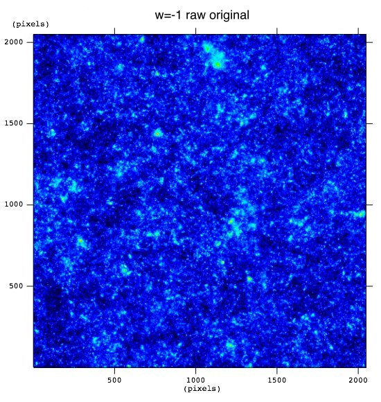
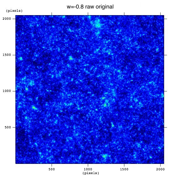
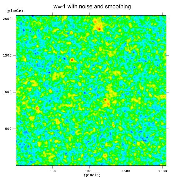
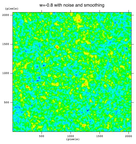
Once the peaks are identified, their heights are recorded in a histogram. This histogram is divided into a reasonable number of bins (the choice in the number of bins will be discussed below), and a vector of values is formed from these bins. We will also attempt to utilize the source galaxy redshifts for tomography, and to combine different smoothing scales, so that each peak is further associated with a value of $z_{s}$ and $\theta_{G}$. Finally, peak identification is repeated in each realization of a given cosmology. We therefore denote the number of peaks in bin $i$ with $N_{i,z_{s},\theta_{G}}^{(f;r)}$, where $f$ and $r$ indicate cosmology and realization, respectively, $z_{s}$ indicates the redshift of the sources and $\theta_{G}$ is the smoothing scale applied to the final map. To simplify notation we hereafter drop the last two lower indices and merge them into the single index $i$.

In order to assess the statistical significance of any difference in peak counts, we construct the covariance matrix $C^{(f)}$ for cosmology $f$ of the counts in the different height-, redshift–, and smoothing–scale bins $i$ and $j$,

$$C_{ij}^{(f)}=\frac{1}{R-1}\sum_{r=1}^{R}(N_{i}^{(f;r)}-\overline{N}_{i}^{(f)})(N_{j}^{(f;r)}-\overline{N}_{j}^{(f)}),$$ (11)

where $\overline{N}_{i}^{(f)}=R^{-1}\sum_{r=1}^{R}{N}_{i}^{(f;r)}$ is the average number of peaks in bin $i$ in the fiducial model $f$, and the summation in equation (11) is over the total number of realizations $R$ constructed for every cosmology.

We use 200 such realizations. However, as noted above, we have run only two strictly independent realizations of each cosmology, i.e., two different simulations with different realizations of the initial conditions. Thus we produce additional pseudo-independent realizations by the standard procedure of randomly rotating, shifting, and slicing the data in the simulation output cubes at each redshift, prior to generating the 2D density planes. Our box–size, $200h^{-1}$Mpc is much larger than the few comoving Mpc correlation length of large–scale structures. As mentioned above, the data cubes are truncated at each output, so that we utilize only a radial slice covering about 1/3rd of its length; the $2.86\times 2.86$ degree field furthermore utilizes only a fraction of this slice. As a result, at intermediate redshifts, where the lensing kernel peaks, each realization utilizes about a twelfth of the volume of the snapshot cube, allowing us to access, in each N–body run, effectively $\sim 12$ truly independent realizations of each lens plane. At the very highest redshift, the situation becomes worse, with up to a third of the volume of the data cubes used. However, due to the distance–dependence of the lensing kernel, the planes near $z_{s}=2$, with these heavily sampled boxes, do not contribute much to the final lensing signal. The random rotations and shifts will create many more than 12 essentially independent random realizations of the incidental line–ups of multiple small clusters and filaments. On the other hand, the very largest clusters – which may create a substantial lensing peak by themselves – will tend to reappear in multiple realizations, and could lead to an underestimation of the variance. Fortunately, our main results come from medium–height peaks, which typically are not caused by a single cluster, so that any such underestimation at the high–convergence end contributes relatively little to our final distinguishing power.

We use the (inverse of) the covariance matrix to compute a value of $\chi^{2}_{f^{\prime}}(r)$ for each realization $r$ of a “test” cosmology, labeled by $f^{\prime}$, against the expectations in the fiducial cosmology, labeled by $f$,

$$\chi^{2}_{f^{\prime}}(r) = \mathbf{dN}^{(f^{\prime};r)}(C^{(f)})^{-1}\mathbf{dN}^{(f^{\prime};r)}$$ (12)

$$= \sum_{ij}dN_{i}^{(f^{\prime};r)}(C^{(f)})_{ij}^{-1}dN_{j}^{(f^{\prime};r)},$$ (13)

where $dN_{i}^{(f^{\prime};r)}\equiv N_{i}^{(f^{\prime};r)}-\overline{N}_{i}^{(f)}$ is the difference between the number of peaks in bin $i$ in realization $r$ of the test cosmology, and the average number of peaks in the same bin in the fiducial cosmology.

The resulting probability distributions for $\chi^{2}_{f^{\prime}}(r)$, using 200 realizations of each cosmology, fixed source redshift $z_{s}=2$ and smoothing scale $\theta_{G}=1^{\prime}$, and 8 peak height bins, is shown in Figure 2. In the top left panel, the realizations were drawn from the simulation of the fiducial $w=-1$ model itself, which was used to compute the mean number of peaks $\overline{N}_{i}^{(f)}$. Our simulated $\chi^{2}$ distribution is very close to a genuine $\chi^{2}$ distribution with $n=8$ degrees of freedom (shown by the black curve). In the bottom left panel, the realizations were again drawn from the $w=-1$ cosmological model, but from the simulation with an independent realization of the initial conditions. The good agreement with the top left panel tests the accuracy of our covariance matrix (in particular, if the covariance had been underestimated, then this second realization would have produced larger $\chi^{2}$ values; see Appendix VI). The two right panels show $\chi^{2}$ distributions computed in the realizations of different cosmologies, with $w=-0.8$ (top right panel), and $w=-1.2$ (bottom right panel). The $w=-0.8$ and $\Lambda$CDM cosmologies are distinguished at the 68% (95%) confidence level in 84% (39%) of the realizations; the $w=-1.2$ cosmology is distinguishable from $\Lambda$CDM at the same confidence in 61% (24%) of the realizations.

For reference, the above confidence levels can be compared to a simpler estimate of the statistical distinction between the two pairs cosmologies, based on the value of $\Delta\chi^{2}_{f^{\prime},f}$, computed using the mean number of peaks in each bin (averaged over all realizations),

$$\chi^{2}_{f^{\prime},f} = \mathbf{dN}^{(f^{\prime},f)}(C^{(f)})^{-1}\mathbf{dN}^{(f^{\prime},f)}$$ (14)

$$= \sum_{ij}dN_{i}^{(f^{\prime},f)}(C^{(f)})_{ij}^{-1}dN_{j}^{(f^{\prime},f)},$$ (15)

where $dN_{i}^{(f^{\prime},f)}\equiv\overline{N}_{i}^{(f^{\prime})}-\overline{N}_{i}^{(f)}$ is the difference between the average number of peaks in bin $i$ in cosmology $f^{\prime}$ and in cosmology $f$. We find $\Delta\chi^{2}=8.35$ between $w=-0.8$ and $w=-1$ (when then same realization of the initial conditions are used in both cosmologies) and $\Delta\chi^{2}=9.54$ (when different realizations are used). The covariance matrix is calculated from the $w=-1$ cosmology in both cases. Assuming that the likelihood distributions are Gaussians, these values would correspond to a $2.8\sigma$ and $3\sigma$ difference between the two cosmologies. This is in good agreement with the 95% exclusion of the mean of the $\chi^{2}$ distribution we find from the individual realizations in the $w=-0.8$ model – indicating that interpreting the $\Delta\chi^{2}$ directly as a probability would only slightly overestimate the statistical difference between the two cosmologies. The corresponding value between the $w=-1.2$ and $w=-1$ models is $\Delta\chi 2=4.65$ (with the same realization of the initial conditions), again confirming that the true likelihood is only somewhat weaker than this simple estimate for the exclusion of the $w=-1.2$ model.

Figure 2: Normalized probability distribution of $\chi^{2}$, computed by comparing the peak counts in individual $3\times 3$ degree convergence fields to the ensemble average in the fiducial $w=-1$ model. Peaks were divided into 8 bins by height. The source galaxies were placed at redshift $z_{s}=2$, and a Gaussian smoothing of $\theta_{G}=1$ arcmin was applied after the addition of ellipticity noise. In the top left panel, the realizations were drawn from the $w=-1$ simulation, the average of which was used to construct the fiducial model. The black curve shows a genuine $\chi^{2}$ distribution with $n=8$ degrees of freedom. In the bottom left panel, the realizations were again drawn from a $w=-1$ model, but from a simulation with different random initial conditions, illustrating that these have a negligible effect on the result for most of the distribution, and testing the accuracy of our covariance matrix. The two right panels show $\chi^{2}$ distributions in different cosmologies, with $w=-0.8$ (top right panel), and $w=-1.2$ (bottom right panel). The $w=-0.8$ and $\Lambda$CDM cosmologies are distinguished at the 68% (95%) confidence level in 84% (39%) of the realizations; the $w=-1.2$ cosmology is distinguishable from $\Lambda$CDM at the same confidence in 61% (24%) of the realizations.

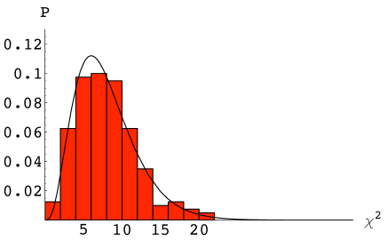
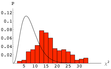
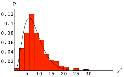
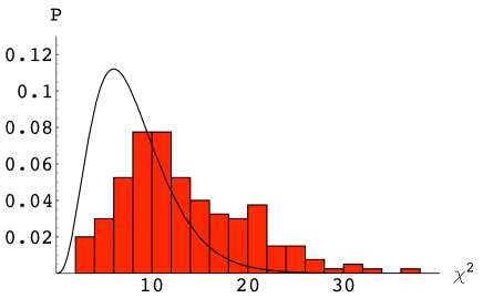
In the above analysis, we have chosen convergence bins whose width was varied, so that they contain approximately equal number of counts ($\approx 350$ peaks/bin at 1 arcmin smoothing). More specifically, the bin boundaries are located at $\kappa=-0.084,0.0022,0.015,0.024,0.032,0.041,0.052,0.068,0.41$. While equal–width bins would perhaps be a more natural choice, the number of peaks falls off exponentially with peak height, and this would have the undesirable result of having many almost empty bins, leading to large $\chi^{2}$ values excessively often (overestimate of improbability of unlikely events), and strong deviations from a true $\chi^{2}$ distribution (since the peak counts do not have a Gaussian distribution, especially for bins with low average counts).

III Weak Lensing Power Spectrum

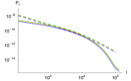
Because our pipeline to produce the WL maps is newly assembled, GADGET-2 was modified to allow $w\neq-1$, and the ray-tracing and WL map analysis codes were newly written, we performed a consistency check, by comparing the power spectrum of the convergence in our maps with the power spectrum derived from semi–analytical predictions. This comparison also determines the range of scales which is adequately represented by our simulations due to resolution and box size. In Figure 3, we show the power spectrum of convergence, averaged over 200 realizations of our simulations (solid curves), together with the theoretical expectations (dashed curves). The latter were obtained by direct line–of–sight integration using the Limber approximation Limber , and using fitting formulas for the nonlinear 3D matter power spectrum from Smith . From top to bottom, the three sets of curves correspond to $w=-1.2$ (green curves), $w=-1$ (red curves), and $w=-0.8$ (blue curves).

We find significant deviations from the theoretical power spectra on both small and large scales, as expected. On small scales, with $\ell\mathrel{\mathchoice{\lower 3.6pt\vbox{\halign{$\mathsurround=0pt\displaystyle\hfill#\hfil$\cr>\crcr\sim\crcr}}}{\lower 3.6pt\vbox{\halign{$\mathsurround=0pt\textstyle\hfill#\hfil$\cr>\crcr\sim\crcr}}}{\lower 3.6pt\vbox{\halign{$\mathsurround=0pt\scriptstyle\hfill#\hfil$\cr>\crcr\sim\crcr}}}{\lower 3.6pt\vbox{\halign{$\mathsurround=0pt\scriptscriptstyle\hfill#\hfil$\cr>\crcr\sim\crcr}}}}20,000$, we are missing power because of the finite resolution on the mass planes and on the ray-tracing grid. On large scales, with $\ell\mathrel{\mathchoice{\lower 3.6pt\vbox{\halign{$\mathsurround=0pt\displaystyle\hfill#\hfil$\cr<\crcr\sim\crcr}}}{\lower 3.6pt\vbox{\halign{$\mathsurround=0pt\textstyle\hfill#\hfil$\cr<\crcr\sim\crcr}}}{\lower 3.6pt\vbox{\halign{$\mathsurround=0pt\scriptstyle\hfill#\hfil$\cr<\crcr\sim\crcr}}}{\lower 3.6pt\vbox{\halign{$\mathsurround=0pt\scriptscriptstyle\hfill#\hfil$\cr<\crcr\sim\crcr}}}}400$, the spectrum is suppressed because of the finite size of the simulation box. These two wave numbers thus set the range, from $\sim 1$ arcmin to $\sim 1$ degree, on which the absolute value of the converge power spectrum is accurately captured.

While we can not trust our results beyond these limits in the subsequent analysis, it should be noted that the ratio of the power spectra in different cosmologies is preserved accurately, even where the simulated power spectra start to deviate from the theoretical predictions. Since we are mainly interested in the comparison between the cosmologies, this makes our results even more robust.

Figure 3: Convergence power spectrum $P(\ell)$, as a function of $\ell=2\pi/\theta$, derived in the three cosmologies (solid blue: $w=-0.8$, solid red: $w=-1$, solid green: $w=-1.2$) from the raw un-smoothed $3\times 3$ degree maps, without ellipticity noise. The simulated power spectra have been averaged over 200 realizations in each cosmology. Also shown are the corresponding semi–analytical predictions based on the matter power spectrum of Smith and using the Limber approximation Limber (dashed curves). The drop around $\ell\sim 20,000$, which corresponds to $\sim 1$ arcmin, is due to the finite resolution of the simulations. The power is also suppressed on large scales, because of finite box size. Note that the ratios of power spectra in the three cosmologies are accurate in the simulations over a wider range than the absolute power.

Another consistency check we perform is a comparison between the number of peaks above a certain threshold to the number of clusters creating lensing peaks above that same threshold. This comparison will presented in Sec. IV.1 below.

IV Results and Discussion

We have found several important quantitative and qualitative results in our study. We first discuss the difference in peak counts between the cosmologies – in the total number of peaks, as well as in the number of peaks in individual convergence bins. We then present our inferred sensitivity to distinguish these cosmologies, and extrapolate this sensitivity from our $3\times 3$ degree field to an LSST–like survey. We discuss the validity of such an extrapolation by studying the variance in peak counts as a function of angular scale. In the next subsection, we comment on correlations between peaks in different bins, with source galaxies at different redshifts, and with different angular smoothing scales, as well as cross-correlations among these. Finally, we briefly contrast our results to other predictions for an LSST–like WL survey, namely constraints from the weak lensing shear power spectrum, the PDF of $\kappa$ found in Wang:2008hi , as well as cluster number counts.

IV.1 Peak Counts

The fundamental quantity we are interested in is the number of peaks in different convergence bins. This quantity is shown in Figure 4 in the three different cosmologies, derived from convergence maps with a single source galaxy plane at $z_{s}=2$, after the addition of ellipticity noise and Gaussian smoothing with $\theta_{G}=1$ arcmin. From top to bottom (at the peak of the distribution), the three curves correspond to $w=-0.8$ (blue curves), $w=-1$ (red curves), and $w=-1.2$ (green curves).

Figure 4: Number of convergence peaks in intervals [$\kappa$, $\kappa+\Delta\kappa$], with $\Delta\kappa=0.0161$ in $3\times 3$ degree fields with source galaxy redshift $z_{s}=2$, 1 arcmin smoothing, and intrinsic ellipticity noise added. From top to bottom (at the peak of the distribution), the three curves correspond to $w=-0.8$ (blue), $w=-1$ (red), and $w=-1.2$ (green). The total number of peaks is 2477, 2432, and 2401, respectively. Notice that the lower distributions have wider wings.

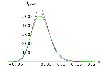
As this figure demonstrates, the distribution of peak heights becomes narrower with increasing $w$.

The total number of convergence peaks in the noisy, smoothed maps is $N_{total}=2432\pm 30$, $N_{total}=2477\pm 30$, and $N_{total}=2401\pm 34$ for $w=-1$, $w=-0.8$, and $w=-1.2$, respectively. Formally, this is a $1.5\sigma$ difference for $w=-0.8$ and a somewhat weaker difference of $1\sigma$ for $w=-1.2$. The same numbers for the smoothed noiseless maps (still with 1 arcmin smoothing) are $N_{total}=1646\pm 24$, $N_{total}=1654\pm 28$, and $N_{total}=1644\pm 24$, respectively. Interestingly, the addition of ellipticity noise boosts both the total number of peaks (by $\sim 50\%$; note that a similar increase was observed by Hamana:2003ts ), and the significance in the difference in peak counts between pairs of cosmologies. Apparently, the number of new peaks introduced by the presence of noise is, itself, $w$–dependent, in a way that helps in distinguishing the two cosmologies.

While this result may first sound surprising, the addition of noise is known boost the discriminating power of related observables. For example, scatter in the mass-observable relation generally increases the number of detectable clusters and tightens constraints from cluster number counts (e.g Haiman et al. (2001)). In our case, one can image that the number of new peaks on 1 arcmin scales, at a given peak height, introduced by the presence of noise, depends on the amplitude of the $\kappa$–fluctuations on larger angular scales, which, itself, is cosmology–dependent. The precise origin of this result will be investigated in a follow-up paper.

Most of the $\sim 2,500$ peaks, of course, have a low amplitude. In order to compare our results with previous work, it is of interest to consider the number of peaks at higher significance. As an example, above the commonly used threshold of $\kappa_{G}=4.5\sigma_{noise}$ (for a source galaxy density of $n_{gal}=15$ arcmin^-2 at redshift $z_{s}=2$, the value of this threshold corresponds to $\kappa_{G}=0.102$ [eq. 9]), the average number of peaks we identify in our 200 pseudo-independent realizations is $N_{\mathrm{peaks}>\kappa_{G}}=47.4\pm 11.8$, $N_{\mathrm{peaks}>\kappa_{G}}=36.6\pm 10.4$, and $N_{\mathrm{peaks}>\kappa_{G}}=54.5\pm 11.4$ for $w=-1$, $w=-0.8$ and $w=-1.2$ respectively, which represent $\approx 1\sigma$ differences between the $w=-1$ and the $w\neq 1$ models. These numbers are with ellipticity noise included. Without ellipticity noise, the number of peaks above the same threshold is $N_{\mathrm{peaks}>\kappa_{G}}=25.9\pm 7.3$, $N_{\mathrm{peaks}>\kappa_{G}}=14.8\pm 5.2$, and $N_{\mathrm{peaks}>\kappa_{G}}=37.0\pm 9.5$, which, again, represent a $1\sigma$ differences. Although the number of these rare high–$\sigma$ peaks is also boosted by the presence of noise, apparently this boost does not enhance the distinguishing power between cosmologies.

It is also useful to compare the number of peaks to the estimated number of clusters causing a convergence signal above the same threshold $\kappa_{G}$. To be closer to predictions in earlier work, for this comparison, we take $n_{gal}=30$ arcmin^-2, resulting in a threshold of $\kappa_{G}=0.072$ for 1 arcmin smoothing. In our noiseless maps, we obtain $N_{\mathrm{peaks}>\kappa_{G}}=99.7\pm 20.0$ and $N_{\mathrm{peaks}>\kappa_{G}}=64.6\pm 14.3$ for $w=-1$ and $w=-0.8$ respectively. To find the corresponding number of clusters, we repeat the calculation in Fang:2006dt , which is based on the fitting formula for the DM halo mass function from Jenkins , and assumes clusters follow the Navarro-Frenk-White profile NFW , but we adjust the cosmological parameters (including the $w$–dependent value of $\sigma_{8}$) to the values adopted here. We find the number of clusters is $N_{\mathrm{clusters}>\kappa_{G}}=48.8\pm 13$, and $N_{\mathrm{clusters}>\kappa_{G}}=31.7\pm 11$ for $w=-1$ and $w=-0.8$, respectively (the errors bars here are approximately twice the $\sqrt{N}$ Poisson errors, enhanced by cosmic variance, following HuKravtsov ). Apparently, there are approximately twice as many convergence peaks in the maps without ellipticity noise as there are clusters, indicating a substantial number of projections. This is roughly consistent with the results of (White et al., 2002; Hamana:2003ts, ; Hennawi:2004ai, ), which self–consistently identify halos in their simulations to quantify this correspondence more reliably, although those works find a somewhat closer correspondence between clusters and $4.5\sigma$ peaks. Adding ellipticity noise increases the number of peaks by another factor of $\sim$two, resulting in plenty of convergence peaks that are not due to a single cluster, which can carry additional information about the cosmology.

An important point to note here is that, as we emphasized earlier, we keep the primordial amplitude fixed as we vary $w$, which leads to a different $\sigma_{8}$ for each $w$. The difference in the average number of clusters (48.8 versus 31.7) quoted above arises essentially entirely from this difference in $\sigma_{8}$. We expect that the difference in peaks counts will similarly be driven primarily by $\sigma_{8}$. Tomography should break some of the degeneracy between $\sigma_{8}$ and $w$; this is an issue that will be clarified and explored in our follow-up work.

IV.2 Three Peak Types

It is instructive to next take a more detailed look at how the number of convergence peaks depends on the peak height, and, in particular, how the counts in different convergence bins vary with cosmology. In the top panel of Figure 5, we show the difference in peak numbers (averaged over the 200 realizations) in $3\times 3$ degree fields in convergence intervals $[\kappa,\kappa+\Delta\kappa]$, with $\Delta\kappa=0.0161$ between the $w=-0.8$ (blue) and the $\Lambda$CDM models, as well as $\Lambda$CDM and $w=-1.2$ (green). The middle panel in the same figure shows the standard deviation in each bin, and the bottom panel depicts the contribution to the $\chi^{2}$ and thus to the distinction power, derived from each bin (note that this bottom panel shows the unequal $\kappa$ bins that were used in our $\chi^{2}$ calculation).

Figure 5: Top Panel: the difference in average peak numbers in each convergence bin is plotted as a function of convergence $\kappa$. The $\Lambda$CDM cosmology is subtracted from $w=-0.8$ (blue) and $w=-1.2$ is subtracted from $\Lambda$CDM (green) in this plot. The height distribution of convergence peaks in $\Lambda$CDM is broader, while in $w=-0.8$ it is narrower, and more sharply peaked (and analogously for $w=-1.2$ vs. $\Lambda$CDM). The numbers plotted are averaged over 200 realizations of a $3\times 3$ degree field, with source galaxies at $z_{s}=2$, 1-arcminute smoothing and the peak heights divided into 50 equal–width convergence bins. Middle Panel: Same as the upper panel, but showing the standard deviation in the number of peaks each bin. Bottom Panel: Contribution to the total $\langle\chi\rangle^{2}$ from the peak number differences in each of the eight convergence bins used in our $\chi^{2}$ calculation. Note that the bins have unequal width, chosen such that each bin contains approximately the same number of peaks (see text). Note that this panel neglects correlations between bins, in order to illustrate the $\kappa$-dependence. There is a small contribution from low peaks, a strong one from medium peaks, and a sizable one from high peaks.

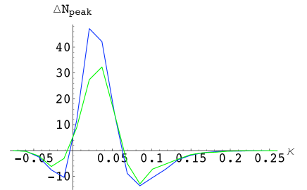
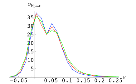
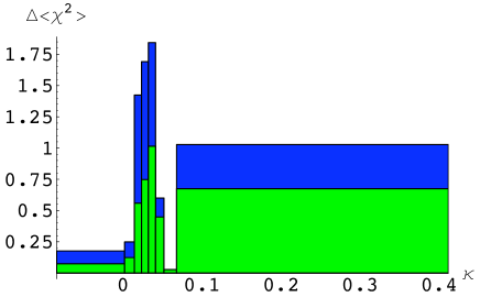
Based on the results shown in this figure, we identify three categories of peaks.

• High Peaks ($\kappa~{}\hbox to0.0pt{$>$\hss}{\lower 4.30554pt\hbox{$\sim$}}0.06$): As is known from previous work (White et al., 2002; Hamana:2003ts, ; Hennawi:2004ai, ), a significant fraction (and perhaps the majority) of these peaks are caused by individual collapsed clusters, which can cause strong peaks by themselves. These peaks are more numerous in cosmologies with more negative $w$. This is as expected: as mentioned above, the more negative $w$ is, the later dark energy starts to dominate the energy density, and the more time massive clusters had to form.

• Medium Peaks ($0.0~{}\hbox to0.0pt{$<$\hss}{\lower 4.30554pt\hbox{$\sim$}}\kappa~{}\hbox to0.0pt{$<$\hss}{\lower 4.30554pt\hbox{$\sim$}}0.06$): The number of these peaks significantly exceeds the expected number of clusters that would cause, by themselves, peaks with a similar height. We examined the contributions of individual lens planes along the line of sight (LOS) to the total convergence in these peaks. We found that for the majority of these peaks, multiple planes contribute significantly, and we therefore suspect these peaks are typically caused by projection along the LOS. In contrast with the high peaks, these medium peaks are more numerous in cosmologies with less negative $w$. This was unexpected. Furthermore, we find that the difference in the counts of these medium peaks dominates the cosmological sensitivity. Clarifying the physical nature of these peaks is important, and will be presented in a follow-up paper Yang:2009 .

• Low Peaks ($\kappa~{}\hbox to0.0pt{$<$\hss}{\lower 4.30554pt\hbox{$\sim$}}0.0$): Similarly to the high peaks, these peaks are more numerous in cosmologies with more negative $w$. However, their number difference compared to their variance is too low to make an appreciable contribution to the distinction between the cosmologies (the number difference of the low peaks is only a fifth of that of the medium peaks, yet their variance still about half). We speculate that these peaks typically reside in “convergence voids” (large areas of the map with very low values of convergence). We have indeed verified that the maps in cosmologies with more negative $w$ show a larger fraction in voids, which gives very low–amplitude peaks a larger area to reside in.

IV.3 Distinguishing $w\neq-1$ Models from $\Lambda$CDM

We use the above difference in peak numbers in bins with different values of $\kappa$ to quantify the statistical distinction between the three models with $w=-1,-0.8$, and $-1.2$. We find that the number of peak height bins used has a minor effect, as long as their number is kept between 4–9. Below this value, the binning is too coarse to capture all the information of the rich structure in the top panel of Figure 5, while higher numbers of bins show signs of over-binning, especially when several source redshifts and smoothing scales are combined (see Appendix VI).

As our fiducial set–up, we use a single source plane at $z_{s}=2$ and $\theta_{G}=1$ arcmin smoothing, as in the previous section. Redshift tomography and using different smoothing scales are addressed in Sec. IV.5 below. The $\chi^{2}$ for each of our $3\times 3$ degree convergence fields (with ellipticity noise and smoothing), compared to the reference cosmology $\Lambda$CDM, is calculated as described in § II.4. This leads to the probability distribution of the $\chi^{2}$ shown in Figure 2.

We can derive our statistical conclusions from these $\chi^{2}$ distributions. For example, the mean of the $\chi^{2}$ distribution for $w=-0.8$ lies at the 95% tail of the $\chi^{2}$ distribution for $w=-1$. This suggests that the $2\sigma$ distinction from a single $3\times 3$ degree field corresponds to $\Delta w=0.2$. The corresponding result for the case of $w=-1.2$ is an exclusion at the 85% confidence level.

IV.4 Extrapolation to an All–Sky Survey

While we are limited by computational costs to studying single $3\times 3$ degree fields, the forthcoming surveys listed in § I will cover much larger areas of the sky - up to $\approx$ 20,000 degree². Therefore, first we would like to extrapolate our results to a larger field of view – or equivalently, translate it to the tighter $2\sigma$ sensitivity to $w$ expected from larger fields.

We will use two methods of extrapolation, an optimistic and a pessimistic one. In the optimistic case, we neglect large-scale correlations and assume that, with increasing survey size, the variance per area–squared in numbers of peaks just falls off as the number of peaks, i.e. $\sigma^{2}_{N_{peak}}\propto N_{peak}$. In the pessimistic case, we extrapolate the scaling of the variance with survey size from the scaling behavior in subfields of our $3\times 3$ degree weak lensing maps. We note that correlations on large scales generally fall off faster than the Poisson–like extrapolation would suggest (Wang:2008hi, ), and in reality, both cases may therefore be conservative estimates.

We illustrate these two methods of extrapolations in Figure 6, where we plot the variance in peak numbers for progressively larger fields, starting with a $1.4\times 1.4$ arcminute field and going all the way to $3\times 3$ degrees (always obtained from our 200 pseudo-independent realizations).

Figure 6: Variance (per area squared) in the total number of convergence peaks, as function of survey area. The red dots denote the variance as measured directly from our $3\times 3$ degree convergence maps and subfields therein, for the $w=-1$ cosmology, with sources at redshift $z_{s}=2$ and 1 arcmin smoothing. The green line shows a power–law fit to the four largest subfields and an extrapolation to a 20,000 degree² field. The black line depicts the slightly more optimistic Poisson–like extrapolation ($\sigma^{2}_{N_{peak}}=N_{peak}$), which ignores long–range correlations. The difference between these two cases causes a factor of 1.3 difference in the extrapolated sensitivity to $w$ on large scales.

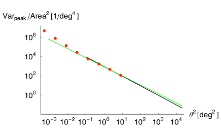
The optimistic extrapolation, shown by the black line in Figure 6, scales to a $\sqrt{20,000/2.86^{2}}=50\times$ stronger sensitivity for a 20,000 degree² field of view. The difference in the dark energy equation of state parameters in our study is $\Delta w=0.2$, which we discern at $2\sigma$. Therefore, roughly, a 20,000 degree² survey will be able to discern a difference of $\Delta w=0.2/50=0.004$ at the same $2\sigma$ level. The somewhat more pessimistic case of extrapolating from existing subfields, as depicted by the green line in Figure 6, yields a variance that is larger by a factor of 1.3. Therefore, for this case, our estimated sensitivity $w$ from an LSST size survey is $\Delta w=0.0052$.

While this is an interesting level of sensitivity, one has to keep in mind that this is a single–parameter constraint, and is not directly comparable to marginalized constraints usually quoted in the literature which fold in degeneracies with other parameters (see § IV.6 below).

IV.5 Different Redshifts and Smoothing Scales

In our fiducial set–up so far, we have used a single source plane ($z_{s}=2$) and smoothing scale ($\theta_{G}=1$ arcmin). Here we examine using other source planes and smoothing scales, including the possibility of using multiple scales in combination.

IV.5.1 Single Redshifts and Smoothing Scale Combinations

We have re–computed $\chi^{2}$ distributions, following the procedure described above, for a variety of different smoothing scales ($\theta_{G}=1,2,3,4,5,10$ arcmin) and source redshifts ($z_{s}=1,1.5,2$). We quote the results by indicating, in each case, the fraction of the realizations of the $w=-0.8$ model which can be excluded from the $w=-1$ cosmology at the 68% (95%) confidence level. These fractions are to be compared to the values of 32% and 5%, expected in the absence of any signal (i.e., for the same cosmology, compared to itself). These fractions are presented in Table 1. We list $\theta_{G}=0.5^{\prime}$ in the table as well, but we caution that, as discussed above, our simulations do not have sufficient resolution to reproduce the convergence power spectrum on these scales, and therefore these results may not be reliable. Unless noted otherwise, we exclude these values from the discussion in the rest of this paper.

% exclusion chance
@ 68 (95)% CL	$z_{s}=1$	$z_{s}=1.5$	$z_{s}=2$
$\theta_{G}=0.5^{\prime}$	48 (13) %	76 (32) %	90 (46) %
$\theta_{G}=1^{\prime}$	56 (16) %	68 (18) %	84 (34) %
$\theta_{G}=2^{\prime}$	53 (12) %	66 (13) %	50 (18) %
$\theta_{G}=3^{\prime}$	41 (10) %	48 (14) %	40 (6) %
$\theta_{G}=4^{\prime}$	39 (6) %	32 (7) %	37 (12) %
$\theta_{G}=5^{\prime}$	38 (6) %	28 (8) %	39 (10) %
$\theta_{G}=10^{\prime}$	26 (2) %	28 (5) %	25 (4) %

Table 1: The probability of distinguishing the $w=-0.8$ model from $\Lambda$CDM, based on peak counts in a single $3\times 3$ degree field, at the 68% (95%) confidence level for various source redshifts $z_{s}$ and smoothing scales $\theta_{G}$, using 8 peak height bins.

There are several trends worth noting in Table 1. First, using source galaxies at high redshift ($z_{s}=2$) provides substantial advantage over using sources at redshift $z_{s}=1.5$ or even $z_{s}=1$ (recall that the surface density is fixed in each case to be 15 arcmin^-2). Dark energy constraints from Type Ia supernovae, and from most other techniques also benefit from deep surveys and high redshifts. For weak lensing, going to higher redshifts is particularly important, as the best lensing efficiency comes from approximately halfway in distance between sources and observer.

Second, as is well known, weak lensing derives most of its power from small scales, and indeed, the smaller the smoothing scale in our maps, the stronger the distinction. This is true down to the smallest angular scales that we can reliable simulate, $\theta_{G}\approx 1$. Smoothing scales larger than $\theta_{G}=2^{\prime}$ do not provide very strong constraints by themselves, but may still be useful when combined with smaller ones (especially for real surveys with much larger fields of view – the number of peaks at these large scales becomes very small for our small $3\times 3$ degree fields).

IV.5.2 Correlations

There are several types of correlations that would be useful to investigate: i.e., correlations in the number of peaks in different height bins, identified for different source redshifts, and with different smoothing scales, as well as the cross-correlations between these quantities. In order to study the effect of these correlations, we computed the $\chi^{2}$ distributions from covariance matrices in which only diagonal elements, or diagonal blocks were retained, and the cross-terms outside these were set to zero.

We find that the peak height bins are correlated. Neglecting all correlations, by retaining only the diagonal elements of the covariance matrix, lead to $\chi^{2}$ histograms that resemble $\chi^{2}$ distributions with fewer degrees of freedom, and an excessive amount of outliers, both typical signs that the dataset contains more correlations than is assumed in the analysis. In particular, as expected, the $\chi^{2}$ distributions (analogous to those shown in Figure 2) develop wider tails toward high $\chi^{2}$ values, with their maximum moving to somewhat smaller values. The net result is that the overlap of the $\chi^{2}$ distributions between a pair of cosmologies is enhanced, and the distinction between the cosmologies is degraded. Table 2 illustrates this in numbers.

% exclusion chance
@ 68 (95)% CL	$z_{s}=1$	$z_{s}=1.5$	$z_{s}=2$
$\theta_{G}=0.5^{\prime}$	32 (1) %	46 (2) %	52 (2) %
$\theta_{G}=1^{\prime}$	34 (2) %	54 (2) %	65 (8) %
$\theta_{G}=2^{\prime}$	40 (3) %	51 (5) %	44 (8) %
$\theta_{G}=3^{\prime}$	39 (2) %	44 (6) %	38 (4) %
$\theta_{G}=4^{\prime}$	36 (2) %	30 (6) %	32 (5) %
$\theta_{G}=5^{\prime}$	32 (4) %	32 (3) %	36 (6) %
$\theta_{G}=10^{\prime}$	24 (2) %	32 (4) %	26 (3) %

Table 2: Same as Table 1, but with correlations between peak height bins neglected. The likelihood of distinguishing $w=-0.8$ from $\Lambda$CDM are much lower, and approach the no-significance values of 32 (5) %, in particular for the 95% confidence level numbers, indicating a large number of outliers.

We also attempted to study cross-correlations between different redshifts and smoothing scales. When studying several redshifts and smoothing scales simultaneously, the number of elements in the covariance matrix grows quickly. Because of the low number of realizations and the corresponding underestimation of the variance, results obtained by using more than $\approx 9$ bins become unreliable (Appendix VI). Unfortunately, this prohibits us from studying the effect of correlations between redshifts and smoothing scales reliably: the number of different peak height bins still allowed becomes too small. In particular, when multiple source redshifts or smoothing scales are simultaneously included, only 2–3 peak heights are allowed by the low number of realizations. We found that such a low number of convergence bins does not sufficiently capture the peak number difference distributions in Figure 5, and no meaningful constraints are possible. We defer a study of these cross–correlations to a follow–up paper, with a larger number of independent realizations of each cosmology.

IV.6 Comparison to Other Forecasts for LSST

It is useful to place our results in the context of constraints expected to be available from other uses of large WL maps. Three methods we will briefly mention here are (i) the shear power spectrum, (ii) cluster number counts, and (iii) the one–point function of the convergence PDF.

(i) From an 11-parameter fit to the tomographic shear power spectrum from LSST and constraints from Planck, Song and Knox (2004) obtain $\sigma(w_{0})=0.06,\sigma(w_{a})=0.09$.

(ii) From a 7-parameter fit to the number counts of $\approx$ 200,000 shear-selected clusters, combined with Planck constraints, SW04 obtain $\sigma(w_{0})=0.04,\sigma(w_{a})=0.09$.

(iii) Using the fractional area statistic of areas of high convergence, Wang:2008hi found $\sigma(w_{0})=0.043,\sigma(w_{a})=0.11$ for LSST and priors from Planck.

The above are all $1\sigma$ constraints, marginalized over a large number of parameters. We do not attempt a fair comparison of the three methods, which would require that identical assumptions are made about the survey specifications and about the set of free parameters (see Albrecht et al. (2006) for a similar exercise covering i. and ii.). Nevertheless, these numbers demonstrate, first, that the statistical information contained in the non–linear features in WL maps – captured by (ii) and (iii) – is at least roughly comparable to the information encoded in the power spectrum in (i). Second, our single–parameter sensitivity to $w$ can be compared meaningfully to those from clusters counts. In particular, as mentioned in § IV.1, the counts of clusters above the $4.5\kappa_{G}$ convergence threshold differs in the $w=-0.8$ and $w=-1$ cosmologies by $\approx 1.5\sigma$. We find that the number of convergence peaks above the same threshold differs in these two cosmologies at a similar, $\approx 1\sigma$ significance level. We find further that considering lower height peaks, with convergence well below this threshold, significantly improves the distinction. While follow-up work, with simulations that address degeneracies between $w$, $\sigma_{8}$, and other parameters is needed, these results suggest that the parameter sensitivity from WL peak counts will be competitive with those from the above three methods.

As mentioned in § I, in a recent preprint, Dietrich:2009jq independently addressed the dependence of WL peaks on the background cosmology. Dietrich:2009jq used the same simulation box size as in our work, but a smaller number of particles ($256^{3}$, rather than $512^{3}$), which allowed them to sample a 2D parameter space and initial conditions, at the cost of mass and angular resolution. They compute the aperture mass for the peaks as a weighted integral of the tangential shear, rather than the convergence. Despite these differences, the conclusions of the two papers appear to be remarkably similar. In particular, if we attribute the distinction we find between our cosmologies with different $w$ values entirely due to the differences in $\sigma_{8}$ in these cosmologies, we find a very similar sensitivity to the latter parameter as their Figure 3: $0.73~{}\hbox to0.0pt{$<$\hss}{\lower 4.30554pt\hbox{$\sim$}}\sigma_{8}~{}\hbox to0.0pt{$<$\hss}{\lower 4.30554pt\hbox{$\sim$}}0.83$ (for a fixed $\Omega_{m}=0.26$). We find, additionally, a subdominant type of peaks – low–amplitude peaks, residing in the voids – the distinction between the cosmologies is however dominated by medium peaks, with a strong contribution from high peaks.

V Summary

We propose the new method of using the counts of peaks, identified in weak gravitational lensing maps, to constrain dark energy and other cosmological parameters. The method makes no reference to cluster counts or their mass function, and so, by definition, is free from selection effects inherent in methods that target clusters.

We used N–body simulations to create theoretical convergence maps in three cosmologies with $w=-0.8$, $w=-1$, and $w=-1.2$. We identify three different peak types: high, medium, and low peaks, whose numbers depend differently on cosmology. The high ($\kappa~{}\hbox to0.0pt{$>$\hss}{\lower 4.30554pt\hbox{$\sim$}}0.6$) and low ($\kappa~{}\hbox to0.0pt{$<$\hss}{\lower 4.30554pt\hbox{$\sim$}}0$) peaks both become more numerous with increasingly negative $w$, while the opposite trend is true for the medium peaks. For the high peaks, this dependence confirms the expectation that when $w$ is more negative, dark energy begins to dominate later, and more time is allowed for the growth of non–linear structures. The opposite behavior of the medium peaks is a surprise - which is all the more important since we find that these peaks dominate the distinction between the cosmologies. The majority of these peaks are not typically caused by individual collapsed clusters, and are more likely due to projection of large scale structure along the line of sight. The low peaks form a subdominant contribution. These peaks are typically due to random ellipticity noise, and we speculate that the larger surface area of voids in cosmologies with more negative $w$, which we have detected in the maps, offers more opportunities for these small fluctuations to arise.

We have shown that based on these peak counts, cosmologies with $w=-0.8$ and $w=-1.2$ can be distinguished from $\Lambda$CDM with a single $3\times 3$ degree convergence field at a 95% and 85% confidence level, respectively. Extrapolating these results to the 20,000 degree² field of view of a large survey, such as LSST, we obtain a projected sensitivity to $w$ of $\Delta w=0.004$–$0.0052$, depending whether the extrapolation is based on the variance measured in subfields of our maps, or whether a simple Poisson–like scaling is used.

In this work, we have explored three constant values of the dark energy equation of state, $w=-0.8$, $w=-1$, and $w=-1.2$, representing variations around the best fit $\Lambda$CDM model to the 5-year WMAP data. The most significant concern is that there will be strong degeneracies between $w$ and other parameters; our results may already be driven primarily by the $\sigma_{8}$ sensitivity in the number of peaks. In a followup paper, we will study such degeneracies; it will also be necessary to perform a larger number of realizations of each cosmology, in order to study the utility of combining several source galaxy redshifts and to use information possibly contained in the angular size distribution of the peaks. In a separate publication Yang:2009 , we also plan to investigate in more detail the physical origin of the three kinds of peaks detected in this work.

VI Appendix: Initial Conditions and the Number of Realizations

In this Appendix, we show our results as a function of the number of peak height bins used, and justify the choice for the number of bins we made in the body of the paper.

Ideally – in the limit that the covariance matrix was perfectly computed – the distinguishing power would asymptotically approach a constant value as one increases the number of bins, at which point using more bins will not provide any more benefit. Unfortunately, it is computationally expensive to generate a large ensemble of initial conditions from which to construct several strictly independent realizations of a given cosmology (a single realization takes approximately 4800 CPU hours, i.e. ca. 2.5 days on 80 CPUs). This, together with the storage required for the large amount of data produced in each run, ultimately limits the number of bins we can utilize.

In particular, using too few realizations, together with too many bins, will generally result in an underestimate of the variance, and an artificial boost in the $\chi^{2}$ values. The possible concern, then, is that the differences we find in the convergence maps between two cosmologies may be caused by such an underestimation of the variance.

In order to guard against this possibility, and to verify that the differences in the convergence maps are caused by genuine differences in cosmology, we generated a second set of independent initial conditions for the cosmologies with $w=-1$ and with $w=-0.8$. The simple Ansatz we adopt for the maximum number of bins that can be safely used, without underestimating variances, is the following: when two different realizations of the same $\Lambda$CDM cosmology are compared, we should recover the $\chi^{2}$ distribution, i.e., we must not be able to rule out the fiducial model itself.

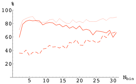
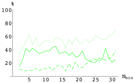
In Figure 7, we show the percentage of the realizations of the $w=-0.8$ test cosmology that lies beyond the 68% (left panel) and 95% (right panel) tail of the $\chi^{2}$ distribution (solid curves), together with the same quantities for the fiducial $\Lambda$CDM cosmology itself (dashed curves). Our Ansatz requires that the dashed curves correspond to the confidence level at which the exclusion is to be achieved (e.g. no more than 32 / 5% of maps excluded at the 68 / 95% confidence level). We see that this condition is satisfied when 4-9 bins are used, but for 10 or more bins, there is a steadily rising difference between the two realizations of the $\Lambda$CDM model. We therefore take 9 bins as the maximum acceptable total number of bins.

Figure 7 also shows that the distinction between $w=-0.8$ and the $\Lambda$CDM model is relatively steady for 4-9 bins, and is insensitive to the choice of the realization of the initial condition. However, for a larger number of bins, the distinction starts to be either less significant (when different realizations of the initial conditions are used in the two cosmologies; solid curves), or begin a modest rise in significance (when the same realizations are used; dotted curves).

While the above analysis is based only on the number of convergence bins, we find similar conclusions when the bins include multiple source galaxy redshifts and/or multiple smoothing scales. We conclude that the accuracy of our covariance matrix limits us to a total of 9 bins.

Figure 7: The solid curves show the percentage of maps in the $w=-0.8$ cosmology which can be excluded at the 68% (left panel) and 95% (right panel) confidence level from $\Lambda$CDM. In these comparisons, the maps in the $w=-0.8$ cosmology were generated from initial condition A, which were compared to the expected average in the $\Lambda$CDM cosmology with initial condition B; the covariance matrix was calculated from $\Lambda$CDM with initial condition A. The dotted curves show the same quantities, except that the maps in the $w=-0.8$ model were taken from initial condition B, and those from $\Lambda$CDM with initial conditions A. The dashed curves again show the same quantities, except maps from the $\Lambda$CDM model (with initial condition B) were compared against $\Lambda$CDM with initial condition A and covariance matrix calculated from initial condition A. If the covariance matrix was correctly estimated, the latter curve should be flat, whereas it is begin to rise systematically for 10 or more bins. Based on this result, we identify 9 as the maximum number of bins that can be safely used without underestimating variances.

References

- Albrecht et al. (2006) Albrecht, A., G. Bernstein, R. Cahn, W. L. Freedman, J. Hewitt, W. Hu, J. Huth, M. Kamionkowski, E. W. Kolb, L. Knox, J. C. Mather, S. Staggs, and N. B. Suntzeff, 2006: Report of the Dark Energy Task Force. e-prints astro-ph/0609591 (2006).
- (2) A. Refregier, Ann. Rev. Astron. Astrophys. 41, 645 (2003). [arXiv:astro-ph/0307212].
- (3) N. Kaiser, J. L. Tonry and G. A. Luppino, arXiv:astro-ph/9912181 (1999).
- (4) J. A. Tyson, D. M. Wittman, J. F. Hennawi and D. N. Spergel, Nucl. Phys. Proc. Suppl. 124, 21 (2003). [arXiv:astro-ph/0209632].
- (5) J. A. Tyson and the LSST Collaboration, Proc. SPIE Int. Soc. Opt. Eng. 4836, 10–20 (2002). See also http://www.lsst.org
- Kaiser (1992) N. Kaiser, “Weak Gravitational Lensing Of Distant Galaxies,”
- Jain and Seljak (1997) B. Jain and U. Seljak, Astrophys. J. 484, 560 (1997).
- Hu (1999) W. Hu, Astrophys. J. 522, L21 (1999).
- Hu (2002) W. Hu, Phys. Rev. D 66, 083515 (2002).
- Huterer (2002) D. Huterer, Phys. Rev. D 65, 063001 (2002).
- Refregier et al. (2004) A. Refregier et al., Astron. J. 127, 3102 (2004).
- Abazajian and Dodelson (2003) K. N. Abazajian and S. Dodelson, Phys. Rev. Lett. 91, 041301 (2003).
- Takada and Jain (2004) M. Takada and B. Jain, Mon. Not. Roy. Astron. Soc. 348, 897 (2004).
- Song and Knox (2004) Y. S. Song and L. Knox, Phys. Rev. D 70, 063510 (2004).
- White et al. (2002) M. J. . White, L. van Waerbeke and J. Mackey, Astrophys. J. 575, 640 (2002).
- (16) T. Hamana, M. Takada and N. Yoshida, Mon. Not. Roy. Astron. Soc. 350, 893 (2004).
- (17) J. F. Hennawi and D. N. Spergel, Astrophys. J. 624, 59–79 (2005).
- Wang and Steinhardt (1998) L. M. Wang and P. J. Steinhardt, Astrophys. J. 508, 483 (1998).
- Haiman et al. (2001) Z. Haiman, J. J. Mohr and G. P. Holder, Astrophys. J. 553, 545 (2001).
- Weller et al. (2002) J. Weller, R. Battye and R. Kneissl, Phys. Rev. Lett. 88, 231301 (2002).
- (21) S. Wang, J. Khoury, Z. Haiman and M. May, Phys. Rev. D 70, 123008 (2004).
- (22) L. Marian, R. E. Smith and G. M. Bernstein, Astrophys. J. 698, L33 (2009).
- (23) T. Chantavat, C. Gordon, and J. Silk, Phys. Rev. D, 79, 083508, (2009).
- (24) W. J. Fang and Z. Haiman, Phys. Rev. D 75, 043010 (2007).
- (25) M. Takada, and S. Bridle, New Journal of Physics, 9, 446 (2007).
- Marian and Bernstein (2006) L. Marian and G. M. Bernstein, Phys. Rev. D 73, 123525 (2006).
- (27) M. Schirmer, T. Erben, M. Hetterscheidt and P. Schneider, Astron. Astrophys. 462, 875 (2007).
- (28) J. P. Dietrich, T. Erben, G. Lamer, P. Schneider, A. Schwope, J. Hartlap and M. Maturi, Astron. Astrophys. 470, 821(2007).
- Jain and Van Waerbeke (2000) B. Jain and L. V. Van Waerbeke, Astrophys. J. 530, L1 (2000).
- (30) S. Wang, Z. Haiman and M. May, Astrophys. J. 691, 547 (2009).
- (31) J. P. Dietrich and J. Hartlap, e-print arXiv:0906.3512.
- (32) V. Springel, Mon. Not. Roy. Astron. Soc. 364, 1105 (2005).
- (33) A. Lewis, A. Challinor and A. Lasenby, Astrophys. J. 538, 473 (2000).
- (34) U. Seljak and M. Zaldarriaga, Astrophys. J. 469, 437 (1996).
- (35) R. W. Hockney, J. W. Eastwood, Adam Hilger, Bristol (1988).
- (36) D. C. Wells, E. W. Greisen and R. H. Harten, Astronomy and Astrophysics Supplement Series 44, 363-370 (1981).
- (37) T. Hamana and Y. Mellier, Mon. Not. Roy. Astron. Soc. 327, 169 (2001).
- (38) S. Dodelson, C. Shapiro and M. J. . White, Phys. Rev. D 73, 023009 (2006).
- (39) L. Van Waerbeke, Mon. Not. Roy. Astron. Soc. 313, 524 (2000).
- (40) D. N. Limber, Astrophys. J. 117, 134 (1953).
- (41) Smith, R. E., J. A. Peacock, A. Jenkins, S. D. M. White, C. S. Frenk, F. R. Pearce, P. A. Thomas, G. Efstathiou, and H. M. P. Couchman, MNRAS, 341, 1311 (2003).
- (42) A. Jenkins et al., Mon. Not. R. Astron. Soc. 321, 372 (2001).
- (43) J. F. Navarro, C. S. Frenk and S. D. M. White, Astrophys. J. 490, 493 (1997).
- (44) W. Hu, & A. V. Kravtsov, Astrophys. J. 584, 702 (2003).
- (45) X. Yang, J. .M. Kratochvil, Z. Haiman, M. May, in preparation.
- (46) S. Pires, J. L. Starck, A. Amara, A. Refregier and R. Teyssier, e-print arXiv:0904.2995