Absence of correlations in the QCD Dirac spectrum at high temperature

Abstract

I propose a simple model of the distribution of the small eigenvalues of the QCD Dirac operator well above the finite temperature phase transition where chiral symmetry is restored and the spectral density at zero vanishes. Assuming the absence of correlations between different regions of the low lying spectrum I derive analytic formulas for the distribution of the first two eigenvalues. I find good agreement with data obtained using the overlap Dirac operator in quenched $SU(2)$ lattice simulations. This suggests that if chiral symmetry is restored spectral correlations are not important and all the statistical properties of the spectrum are encoded in the spectral density.

Random Matrix Theory (RMT) has been rather successful in describing some universal properties of the spectrum of the QCD Dirac operator Verbaarschot:2000dy . Most of the results, however, concern the chirally broken phase of the theory. This regime is characterized by a non-zero density of eigenvalues around zero, which through the Banks-Casher relation leads to a non-vanishing chiral condensate. Using a single parameter, the value of the chiral condensate, RMT makes detailed predictions about the distribution of the smallest Dirac eigenvalues.

Above the finite temperature phase transition, $T_{c}$, the Dirac spectrum is much less understood in terms of RMT. Multicritical random matrices with fine tuning in the action might be able to describe the chirally restored phase Akemann:1997wi . Another possibility is to add a temperature dependent constant matrix to the usual chiral random matrix to mimic the lowest Matsubara mode Jackson:1995nf ; Stephanov:1996he . For comparisons with lattice staggered data above $T_{c}$ see Refs. Farchioni:1999ws . Recently there has also been renewed interest in a better understanding of the Dirac spectrum around and above $T_{c}$ with the hope of clarifying the connection between the chiral and deconfinement transition Gattringer:2006ci .

In the present paper I propose a model of the low lying Dirac spectrum that can provide a simple alternative to RMT well above $T_{c}$ . The main assumptions I make for the Dirac spectrum around zero are the following:

1. For fixed temperature the spectral density scales with the spatial volume.
   

2. The spectral density per unit spatial volume is

   $$\rho(\lambda)=C\lambda^{\alpha},$$ (1)

   where $C$ and $\alpha$ are constants.
   

3. The number of eigenvalues in any two disjoint intervals are independent random variables.

Using lattice data from quenched $SU(2)$ simulations with the overlap Dirac operator I directly verify assumptions (1) and (2). Based on (1-3) I derive analytic formulas for the statistical properties of the first two eigenvalues in terms of $C,\alpha$ and the spatial volume. Fitting $C$ and $\alpha$ to the lattice data, the analytic formulas provide several parameter-free predictions and I find perfect agreement with the numerical lattice data.

Table 1: The number of configurations $N$ generated for the different spatial box sizes $L$. $N_{Q=0}$ is the number of configurations in the trivial topological sector, the one used here.

$L$	12	14	16	18	20	22	24	32
$N$	900	850	738	400	490	326	376	42
$N_{Q=0}$	879	821	711	379	451	298	328	29

At first I summarize the details of the numerical simulations. The data is based on quenched simulations of the $SU(2)$ gauge theory with Wilson plaquette coupling $\beta=2.6$ and time extension $N_{t}=4$. This corresponds to a temperature of about $T=2.6T_{c}$, well above the finite temperature phase transition. The spatial size of the box was chosen in the range $N_{s}=12-32$, spanning more than an order of magnitude in spatial volume (see Table 1). In eight different spatial volumes I computed the 16 (or 32) eigenvalues of smallest magnitude of the overlap Dirac operator Narayanan:ss ,

$$D_{\mbox{\scriptsize ov}}=1-A\left[A^{\dagger}A\right]^{-\frac{1}{2}},\hskip 28.45274ptA=1+s-D_{0},$$ (2)

where $D_{0}$ is the Wilson Dirac operator and I use $s=0.4$ that appears to be optimal for the condition number of $A^{\dagger}A$. The spectrum of the Dirac operator is symmetric with respect to the real axis and I only consider the eigenvalues with non-negative imaginary parts. The overlap Dirac operator has an exact chiral symmetry and its spectrum lies along a circle touching the origin. The eigenvalues of smallest magnitude therefore have only small real parts and the low end of the spectrum is much like that of the continuum Dirac operator which has a purely imaginary spectrum. In the analysis I always use only the imaginary part of the eigenvalues.

The low-end of the Dirac spectrum is known to depend strongly on the temporal fermionic boundary condition which is effectively a combination of the Polyakov loop and the explicitly chosen anti-periodic boundary condition Bilgici:2009tx . In the quenched $SU(2)$ theory the Polyakov loop $Z(2)$ symmetry is spontaneously broken above the critical temperature. While in the negative Polyakov loop sector there is a non-zero density of eigenvalues around zero (as if chiral symmetry were broken), in the positive sector there seems to be a gap roughly controlled by the lowest Matsubara frequency Kovacs:2008sc . Although in the quenched theory the two sectors are equivalent, I will restrict my study to the latter, the one that survives in the high temperature phase in the presence of dynamical fermions since they explicitly break the $Z(2)$ symmetry. The boundary conditions I use for the fermions are always anti-periodic in the time direction and periodic in all the spatial directions.

In addition to the small non-zero modes, due to its exact chiral symmetry, the overlap operator can also have exact zero modes, regardless of the boundary condition or the Polyakov loop sector. I use only configurations belonging to the trivial topological sector which is the most abundant in these simulations (see Table 1).

Figure 1: The cumulative spectral density scaled by the 3-volume for all eight 3-volumes. The dashed line is the analytic prediction using the parameters fitted for the average smallest eigenvalue. The difference between Fig. (a) and (b) is that while in the former we assume no gap for the fitting, in the latter a gap $G=0.39$ is assumed.

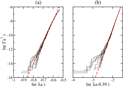
(1) Scaling of the spectral density— In Fig. 1 I plot the cumulative spectral density normalized by the spatial volume,

$$\Gamma(\lambda)=\int_{0}^{\lambda}dx\,\rho(x),$$ (3)

for different spatial box sizes. $\Gamma(\lambda)$ is the average number of eigenvalues per unit volume smaller than $\lambda$. The densities in the different volumes agree perfectly except for the very low end where the data is sparse and statistical errors are large. The scaling of the spectral density with the 3-volume is a rather non-trivial property of the interacting theory. For free fermions the level spacing is inversely proportional to the linear box size since the Dirac equation is first order. That would imply a spectral density scaling with the linear size, not the volume.

(2) Form of the spectral density— As can be seen in the log-log plot of $\Gamma$, the integrated spectral density versus $\lambda$ (Fig. 1a), the data is well described by the simple power law of Eq. (1) therefore I will assume that in what follows.

I emphasize that for the main result of the paper the particular form of the spectral density is immaterial. The whole forthcoming analysis can be carried out with any simple analytic form of the spectral density that describes the data accurately. In particular there are also expectations based partly on RMT Jackson:1995nf and lattice data Gattringer:2002tg that at high temperature, well above $T_{c}$ the spectrum develops a gap $G$ around zero. In that case the spectral density would be expected to start off from $G$ as

$$\rho(\lambda)=C(\lambda-G)^{\alpha}.$$ (4)

Later I will also discuss this possibility. Potentially the accumulation of small non-zero eigenvalues seen in Edwards:1999zm might also complicate the picture, but the temperature used here is high enough that these modes are completely absent, at least with the present statistics.

(3) No spectral correlations— i.e. the number of eigenvalues in any two disjoint intervals are independent random variables. This is the most non-trivial of the three assumptions and the demonstration of its validity is the main result of the paper. I will show that the resulting description fits the numerical data rather accurately. The absence of correlations between different regions of the spectrum immensely simplifies any model since it means that all probabilistic information about the spectrum is encoded in the spectral density. All the properties of the low eigenvalues follow from a simple few-parameter description of the spectral density like Eq. (1) or (4).

It is important to note that the absence of correlations between different regions of the spectrum is not related in any simple way to the correlations between individual eigenvalues that is often considered in random matrix models Akemann:2003tv . In particular it does not imply the absence of correlations between individual eigenvalues.

Distribution of the smallest eigenvalues— I now compute the distribution of the smallest two eigenvalues from assumptions (1-3). From the definition of the spectral density $V\rho(\lambda)d\lambda$ is the average number of eigenvalues in spatial volume $V$ in an interval of length $d\lambda$ centered around $\lambda$. If at fixed volume the length of the interval $d\lambda\rightarrow~{}0$ then the probability of having one eigenvalue in the interval is $V\rho(\lambda)d\lambda$ and the probability of no eigenvalue is $1-V\rho(\lambda)d\lambda$. This is because the probability of having more than one eigenvalue becomes negligible.

Let us first compute the probability $P_{no}(\lambda_{1},\lambda_{2})$ that there is no eigenvalue in the interval $[\lambda_{1},\lambda_{2}]$. Since correlations between the subintervals are ignored the probability of having no eigenvalue in an interval can be written as the product of probabilities of having no eigenvalue in any subinterval of its decomposition into small subintervals.

$$P_{no}(\lambda_{1},\lambda_{2})=\lim_{\Delta x\rightarrow 0}(1-V\rho(x_{1})\Delta x)\;(1-V\rho(x_{2})\Delta x)\;...$$

$$(1-V\rho(x_{N})\Delta x),$$ (5)

where $x_{1}=\lambda_{1}$, $x_{N}=\lambda_{2}$ and $x_{k+1}-x_{k}=\Delta x$. Expanding the product the terms can be organized in powers of $\Delta x$ and in the limit $\Delta x\rightarrow 0$ the order $n$ term goes to the following $n$-fold integral;

$$S_{n}=(-V)^{n}\int_{\lambda_{1}}^{\lambda_{2}}dx_{1}\rho(x_{1})\int_{x_{1}}^{\lambda_{2}}dx_{2}\rho(x_{2})\;...\;$$

$$\int_{x_{n-1}}^{\lambda_{2}}dx_{n}\rho(x_{n}).$$ (6)

Substituting the spectral density in Eq. (1) for $\rho$ the integrations can be explicitly carried out resulting in

$$S_{n}=\frac{(-CV)^{n}}{n!(\alpha+1)^{n}}\left(\lambda_{2}^{\alpha+1}-\lambda_{1}^{\alpha+1}\right)^{n}.$$ (7)

Finally the summation over $n$ is easily done giving

$$P_{no}(\lambda_{1},\lambda_{2})=\exp\left(-\frac{CV}{\alpha+1}(\lambda_{2}^{\alpha+1}-\lambda_{1}^{\alpha+1})\right)$$ (8)

for the probability of no eigenvalue in the interval $[\lambda_{1},\lambda_{2}]$.

Using again assumption (3) the probability of having the smallest eigenvalue around $\lambda$ is the product of two probabilities: having no eigenvalue in $[0,\lambda]$ and having one eigenvalue in $[\lambda,\lambda+d\lambda]$. Thus the probability density of the smallest eigenvalue is

$$\rho_{1}(\lambda)=\exp\left(-\frac{CV}{\alpha+1}\lambda^{\alpha+1}\right)CV\lambda^{\alpha}.$$ (9)

The average smallest eigenvalue is easily calculated from this as

$$\langle\lambda_{1}\rangle=\int_{0}^{\infty}\rho_{1}(x)x\;dx=(CV\mu)^{-\mu}\;\Gamma(1+\mu),$$ (10)

where I introduced the notation $\mu=(1+\alpha)^{-1}$.

The distribution and average of the second smallest eigenvalue can be calculated in a similar fashion. Again the probability of having the second eigenvalue around $\lambda$ can be decomposed as a product: having the smallest eigenvalue at $x$, having no eigenvalues between $x$ and $\lambda$ and having an eigenvalue around $\lambda$. Since $x$ (the occurrence of the first eigenvalue) can be anywhere between 0 and $\lambda$, $x$ has to be integrated and the probability density of the second eigenvalue is

$$\rho_{2}(\lambda) = \int_{0}^{\lambda}dx\;\rho_{1}(x)\;P_{no}(x,\lambda)\;\rho(\lambda)$$ (11)

$$= \frac{C^{2}V^{2}}{\alpha+1}\exp\left(-\frac{CV}{\alpha+1}\lambda^{\alpha+1}\right)\,\lambda^{2\alpha+1}.$$

Finally we obtain

$$\langle\lambda_{2}\rangle=(CV\mu)^{-\mu}\;\Gamma(2+\mu),$$ (12)

for the average second eigenvalue. The procedure can be easily continued for higher eigenvalues.

Figure 2: The average smallest and second smallest eigenvalue as a function of the spatial volume in lattice units. The solid curve is a two-parameter fit of the form Eq. (10). The dashed curve is the fitted parameter-free prediction for the average second smallest eigenvalue.

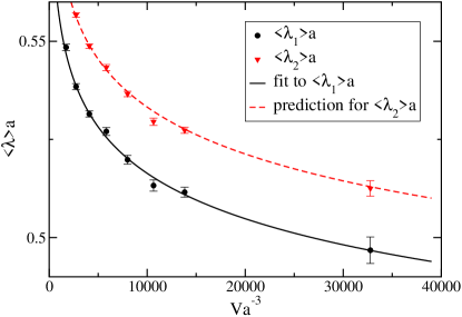
Numerical results and tests— In the remainder I compare the analytic formulas and the data. There are many different ways to proceed; one has to fit the two parameters $C$ and $\alpha$ in the spectral density using any of the analytic formulas above and then the rest of the formulas are predictions that can be tested against the data. I choose to use Eq. (10), the scaling of the average smallest eigenvalue with the 3-volume $V$ for the fit. Using a fit range of $V=14^{3}-32^{3}$ produces a good fit with $\chi^{2}$/d.o.f.$=0.89$. The parameters obtained are $C=1.07(82)\times 10^{6}$ and $\mu=\frac{1}{\alpha+1}=0.0327(12)$. In Fig. 2 I plotted the average smallest eigenvalue as a function of the 3-volume along with the fit. Also in this Figure I present the average second eigenvalue and the analytic formula of Eq. (12) using the above parameters. Notice that this is now a prediction of the model with no further parameters to be fitted and it agrees quite well with the data.

Figure 3: The distribution of the smallest and second smallest eigenvalues in a spatial volume of $V=16^{3}$. The solid lines indicate the analytic prediction of the model (Eqs. (9) and (11)).

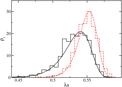
A more detailed prediction is the distribution of the smallest and second smallest eigenvalue for different spatial volumes. As an illustration, Fig. 3 shows this in a spatial volume of $V=16^{3}$ and again there is good agreement with the data. The picture is similar for the other volumes down to $V=14^{3}$ below which even the distribution of the smallest eigenvalue starts to be concentrated above the upper limit of the validity of the simple power-law of Eq. (1) for the spectral density.

Is there a spectral gap?— Coming back to the question of whether there is a spectral gap, the derivation of the distributions can be easily generalized for the spectral density of Eq. (4) yielding

$$\langle\lambda_{1}\rangle=(CV\mu)^{-\mu}\;\Gamma(1+\mu)\;+\;G$$ (13)

for the average smallest eigenvalue. Unfortunately a three-parameter fit—including $G$—to the average smallest eigenvalue is not very meaningful since in a wide range of $G$ almost equally good fits can be found for $C$ and $\alpha$. We can, however, assume that $G$ is somewhat smaller than the smallest observed eigenvalue. In our simulation data for the eight different spatial volumes comprising altogether more than 4000 configurations the smallest eigenvalue was 0.3965. If a gap of $G=0.39$ is assumed, the fit yields $C=5.4(3.6)\times 10^{3}$ and $\mu=0.1275(52)$ with $\chi^{2}/$d.o.f.$=1.03$. Comparing the predicted cumulative spectral density with the data on a log-log plot (Figs. 1a and 1b) shows that the cumulative spectral density definitely favors $G=0$ over $G=0.39$, however, a much smaller but still non-zero value of the gap cannot be ruled out based on the present data.

Discussion— We proposed a description of the low-lying Dirac spectrum at high temperature based on the assumption that there are no correlations between different regions in the spectrum. Our model provides detailed analytic predictions for the distribution of the low-lying Dirac eigenvalues and perfect agreement is found with numerical lattice data. The absence of correlations is a peculiar property of the chirally symmetric phase and is not expected to hold if chiral symmetry is broken. It would be interesting on the one hand to get a more fundamental understanding of this property and on the other hand to see whether it is shared by a wider class of chirally symmetric systems. A good testing ground could be the Schwinger model with two flavors of massless fermions Bietenholz:2009jn . The model proposed here might eventually provide a full description of the Dirac spectrum in the chirally restored phase, just like Random Matrix Theory in the chirally broken phase. Together with RMT it might also open the possibility to a better understanding of the nature of the chiral phase transition of QCD and even the conformal phase of QCD-like theories with more fermionic degrees of freedom DeGrand:2009et .

References

- (1) J. J. M. Verbaarschot and T. Wettig, Ann. Rev. Nucl. Part. Sci. 50, 343 (2000) [arXiv:hep-ph/0003017].
- (2) G. Akemann, P. H. Damgaard, U. Magnea and S. M. Nishigaki, Nucl. Phys. B 519, 682 (1998) [arXiv:hep-th/9712006].
- (3) A. D. Jackson and J. J. M. Verbaarschot, Phys. Rev. D 53, 7223 (1996) [arXiv:hep-ph/9509324].
- (4) M. A. Stephanov, Phys. Lett. B 375, 249 (1996) [arXiv:hep-lat/9601001]; M. A. Nowak, G. Papp and I. Zahed, Phys. Lett. B 389, 341 (1996) [arXiv:hep-ph/9604235].
- (5) F. Farchioni, P. de Forcrand, I. Hip, C. B. Lang and K. Splittorff, Phys. Rev. D 62, 014503 (2000) [arXiv:hep-lat/9912004]; P. H. Damgaard, U. M. Heller, R. Niclasen and K. Rummukainen, Nucl. Phys. B 583, 347 (2000) [arXiv:hep-lat/0003021].
- (6) C. Gattringer, Phys. Rev. Lett. 97, 032003 (2006) [arXiv:hep-lat/0605018]; F. Bruckmann, C. Gattringer and C. Hagen, Phys. Lett. B 647, 56 (2007) [arXiv:hep-lat/0612020].
- (7) C. Gattringer and S. Schaefer, Nucl. Phys. B 654, 30 (2003) [arXiv:hep-lat/0212029].
- (8) R. Narayanan and H. Neuberger, Phys. Rev. Lett. 71 (1993) 3251 [arXiv:hep-lat/9308011]. Nucl. Phys. B 412, 574 (1994) [arXiv:hep-lat/9307006]; Nucl. Phys. B 443, 305 (1995) [arXiv:hep-th/9411108].
- (9) E. Bilgici, F. Bruckmann, J. Danzer, C. Gattringer, C. Hagen, E. M. Ilgenfritz and A. Maas, arXiv:0906.3957 [hep-lat].
- (10) R. G. Edwards, U. M. Heller, J. E. Kiskis and R. Narayanan, Phys. Rev. D 61, 074504 (2000) [arXiv:hep-lat/9910041].
- (11) T. G. Kovacs, PoS LATTICE2008, 198 (2008) [arXiv:0810.4763 [hep-lat]].
- (12) G. Akemann and P. H. Damgaard, Phys. Lett. B 583, 199 (2004) [arXiv:hep-th/0311171].
- (13) T. DeGrand, arXiv:0906.4543 [hep-lat]; Z. Fodor, K. Holland, J. Kuti, D. Nogradi and C. Schroeder, arXiv:0908.2466 [hep-lat].
- (14) W. Bietenholz and I. Hip, arXiv:0909.2241 [hep-lat].