Competition for Popularity in Bipartite Networks

Abstract

We present a dynamical model for rewiring and attachment in bipartite networks in which edges are added between nodes that belong to catalogs that can either be fixed in size or growing in size. The model is motivated by an empirical study of data from the video rental service Netflix, which invites its users to give ratings to the videos available in its catalog. We find that the distribution of the number of ratings given by users and that of the number of ratings received by videos both follow a power law with an exponential cutoff. We also examine the activity patterns of Netflix users and find bursts of intense video-rating activity followed by long periods of inactivity. We derive ordinary differential equations to model the acquisition of edges by the nodes over time and obtain the corresponding time-dependent degree distributions. We then compare our results with the Netflix data and find good agreement. We conclude with a discussion of how catalog models can be used to study systems in which agents are forced to choose, rate, or prioritize their interactions from a very large set of options.

Human dynamics, which is concerned with the characterization of human activity in time, has been the subject of intense and exciting research over the last few years barabasi-2005-435 ; evans-2008-3 ; J.P.Onnela05012007 . In one typical problem setting, individuals are endowed with limited resources, and there are numerous activities, behaviors, and/or products that compete against each other for those resources. Although such situations admit a natural formulation using bipartite (two-mode) networks that connect individuals to activities, human dynamics has surprisingly seldom been studied from this perspective. In the present paper, we analyze bipartite networks constructed from a large data set of video ratings by the users of a video rental company over a period of six years. To analyze the time evolution of these networks, we introduce the concept of a catalog network, and we use this approach to explore the driving forces behind the video rating behavior of individuals. We believe that such a framework can be used to study many other phenomena in human dynamics that involve the allocation of and competition for scarce resources.

I Introduction

Numerous natural and man-made systems involve interactions between large numbers of entities. The structural configuration of interactions is typically rather complicated, so the study of such systems often benefits greatly from network representations albert-2002-74 ; Newman:2003 ; guido . A network is usually abstracted mathematically as a graph whose nodes represent the entities and whose edges represent the interactions between the entities HandbookGraphTheory . In many cases, edges can be weighted or directed, and more complicated frameworks such as hypergraphs can also be employed. The number of edges connected to a node in an unweighted network is known as its degree, and the degree distribution of a network is given by the collection of numbers that give the fraction of nodes that have degree $k$ (for all values of $k$) Newman:2003 . In weighted networks, one considers the weight of an edge rather than simply whether or not it exists.

Because networked systems are not static, the last decade has witnessed a particular interest in models that attempt to address their growth and evolution guido . Perhaps the best-known model of network growth was formulated by Barabási and Albert BarabasiAlbert1999 ; albert-2002-74 . Similar models were also constructed decades earlier by Simon HERBERTA.SIMON12011955 and Price Price:1965 . Barabási and Albert examined networks arising from diverse settings and found that their degree distributions often seemed to follow power laws, which are functions of the form $f(x)\sim x^{-\alpha}$ (with $\alpha>0$). They proposed a growth mechanism, which they called preferential attachment (Price had called it cumulative advantage) to try to explain their observations. One starts with a small seed network and—in the simplest form of the mechanism—iteratively adds individual nodes that each possess exactly one edge. One connects each new node to an existing one chosen at random with probability proportional to its degree. That is, the probability to choose node $m_{i}$ with degree $k_{i}$ is

$$P(m_{i})=\frac{k_{i}}{\sum_{j=1}^{N}k_{j}}\,,$$

where the total number of nodes $N$ indicates the size of the network. Because nodes with higher degrees have correspondingly higher probabilities to receive new edges, the preferential attachment growth mechanism leads naturally to a power-law degree distribution BarabasiAlbert1999 ; PhysRevLett.85.4629 .

Because of ideas like preferential attachment and the resulting insights on the origin of heavy-tailed degree distributions that one sees, e.g., in the World Wide Web or scientific collaboration networks, the study of networks has grown immensely during the last ten years Newman:2003 ; NewmanSciCol ; guido . However, most of this research has concentrated on one-mode (unipartite) networks, in which all of the nodes are of the same type. It is perhaps under-appreciated that other graph structures are also very important in many applications Latapy200831 . Even the simplest generalization, known as a two-mode or bipartite network, has been studied much more sparingly than unipartite networks. Bipartite networks contain two categories (partite sets) of nodes: $\mathcal{U}=\{u_{1},u_{2},\dots,u_{U}\}$ (with $U$ members) and $\mathcal{M}=\{m_{1},m_{2},\dots,m_{M}\}$ (with $M$ members). As shown in Fig. 1, each (undirected) edge connects a node in $\mathcal{U}$ to one in $\mathcal{M}$ HandbookGraphTheory . Bipartite networks abound in applications: They can represent affiliation networks in which people are connected to organizations or committees MasonPorter05172005 , ecological networks with links between cooperating species in an ecosystem Saavedra07532 , and more Zhang20086869 ; Guillaume04bipartitegraphs ; PhysRevE.72.036120 ; evans:056101 ; baseball .

Figure 1: (Color online) A bipartite network with nodes in the partite sets $\mathcal{U}=\{1,2,3,4\}$ and $\mathcal{M}=\{A,B,C\}$. Each edge connects a number to a letter.

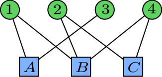
A bipartite network possesses a degree distribution for each of the two node types. We denote the adjacency matrix of a weighted bipartite network by $\mathbf{G}\in\mathbb{R}^{U\times M}$. Each matrix element $\mathbf{G}_{ij}$ has a nonzero value if and only if an edge exists between nodes $u_{i}$ and $m_{j}$. We denote the matrices that result from the two unipartite projections as $\mathbf{G}_{\mathcal{U}}=\mathbf{G}\mathbf{G}^{T}\in\mathbb{R}^{U\times U}$ and $\mathbf{G}_{\mathcal{M}}=\mathbf{G}^{T}\mathbf{G}\in\mathbb{R}^{M\times M}$. The degree of a node in a unipartite projection network is then the number of nodes of the same type with which the node shares at least one neighbor in the original bipartite network. The node strengths similarly incorporate connection strengths from the original bipartite network. (Recall that the “strength” of a node is the sum of the strengths of the edges connected to it.) For example, in an unweighted affiliation network, the two projections give the weighted connection strength (the number of common affiliations) among individuals and the interlock (the number of common people) among organizations ceo ; MasonPorter05172005 .

Many of the real-life systems that can be represented by bipartite networks are dynamic, as the existence and connectivity of both nodes and edges can change in time. For example, a person might retire or leave one organization to join another. One of the simplest types of changes is edge rewiring, in which one end of an edge is fixed to a node and the other end moves from one node to another (such as in the aforementioned change of affiliation). Because of the important insights they can offer, network rewiring models have received increasing attention WattsStrogatz ; PhysRevE.72.036120 ; evans:056101 ; Dorogovtsev2003396 ; PhysRevE.72.026131 ; fan026103 ; lind . They are closely related to abstract urn models from probability theory polya ; feller ; Godreche0953 , models of language competition Stauffer2007835 , and models of transmission of cultural artifacts Bentley2003 . More generally, they can help lead to a better understanding of any system in which the nature or existence of an interaction among agents changes over time evans-2008-3 .

The rest of our presentation is organized as follows. In Section II, we analyze a large data set of time-stamped video ratings from the video rental service Netflix that we model as a bipartite network of people and videos. In Section III, we examine the bursty behavior of individual users. In Section IV, we develop a catalog model of bipartite network growth and evolution. We then study the Netflix data using this model in Section V. Finally, we discuss our results and present directions for future research in Section VI.

II Netflix Video Ratings

Netflix is an online video rental service that encourages its users to rate the videos they rent in order to improve their personalized recommendations. As part of the Netflix Prize competition Netflixprize , in which the company challenged the public to improve their video recommendation algorithm, Netflix released a large, anonymized collection of user-assigned ratings of videos in its catalog. In this paper, we use the Netflix data to study human dynamics in the form of video ratings from a limited catalog. One can also examine the dynamics of the ratings themselves, which would complement a recent empirical study of video ratings that used data from the Internet Movie Database (IMDB) imdb . The Netflix data consist of 100,480,507 ratings of 17,770 videos. The ratings, which were given by 480,189 Netflix users between October 1998 and December 2005, were sampled uniformly at random by Netflix from the set of users who had rated at least 20 videos netflixPaper . Each entry in the data includes the video ID, user ID, rating score (an integer from 1 to 5), and submission date. To illustrate some of the temporal dynamics in the data, we show in Fig. 2 the total number of ratings for each day from July to August 2003. The number of daily ratings exhibits a weekly pattern in which Mondays and Tuesdays have the highest activity and Saturdays and Sundays have the lowest. This reflects the weekly patterns in human work–leisure habits.

Figure 2: Number of daily ratings for each day in July and August 2003. The mean number of ratings per day over this period is 30,449. The dashed vertical lines indicate Tuesdays.

Figure 3: (Color online) Number of ratings in the Netflix data versus time from the beginning of 2000 to the end of 2005. Circles indicate data from Netflix and the dashed red curve is a fit to equation (1).

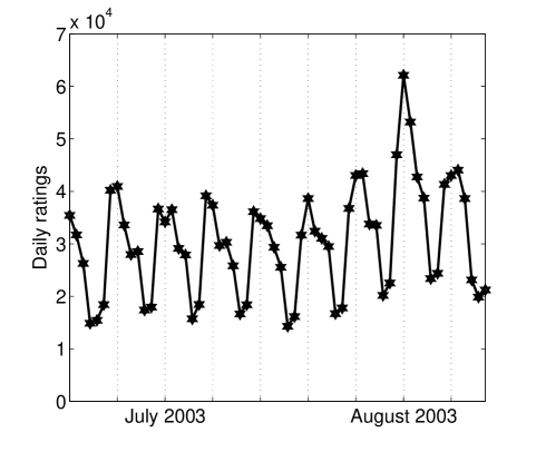
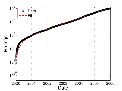
Figure 3 shows the total number of ratings from 2000 to the end of 2005. These ratings seems to grow exponentially, which we confirm by fitting the data to the function

$$r(t)=a_{r}\left(e^{b_{r}t}-1\right)$$ (1)

using nonlinear least squares. We obtain the parameter values $a_{r}\approx 6.3656\times 10^{5}$ and $b_{r}\approx 0.0024$.

Figure 4: (Color online) Number of users (top) and videos (bottom) in the Netflix data versus time from the beginning of 2000 to the end of 2005. Circles indicate data from Netflix and the dashed red curves are fits to equations (2) and (3) for users and videos, respectively.

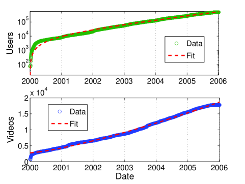
The number of users also grows exponentially, as shown on the top panel of Fig 4. The dashed curve in the plot is the fit to

$$u(t)=a_{u}(e^{b_{u}t}-1)\,,$$ (2)

where we obtain $a_{u}\approx 1.0018\times 10^{4}$ and $b_{u}\approx 0.0018$. We will need to take the exponential growth of the system into account when comparing data from dates that are far apart from each other.

In the bottom panel of Fig. 4, we show the number of videos from 2000 to 2005. The number of videos appears to grow roughly linearly as a function of time, but in fact it is better described by the relation

$$m(t)=a_{m}+b_{m}t^{c_{m}}\,,$$ (3)

where fitting yields $a_{m}\approx 2780.00$, $b_{m}\approx 0.6705$, and $c_{m}\approx 1.3097$.

II.1 Bipartite Network Formulation

The Netflix data can be represented as a bipartite network. The two types of nodes in this network are users and videos. We use $\mathcal{U}$ to denote the set of users and $\mathcal{M}$ to denote the set of videos. We ignore the rating values and consider only the presence or absence of a rating event, which corresponds to an edge between a user and a video in the unweighted bipartite network. The large size and longitudinal nature of the data provides a valuable opportunity to study video rating in the context of human dynamics, as has been done previously with mobile telephone networks J.P.Onnela05012007 ; nature06958 , book sale rankings Sornette.93.228701 , and electronic and postal mail usage patterns barabasi-2005-435 ; oliveira2005437 .

II.2 Degree Distributions

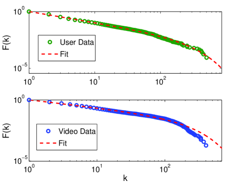
The bipartite video-rating network has one degree distribution for the user nodes and another one for the video nodes. Keeping in mind the observations in Fig. 2, we examine the cumulative degree distributions of individual days. The distributions have a similar functional form for each day in the data set. We fit them to a power law with an exponential cutoff,

$$F(k)\sim k^{-a}e^{-bk}\,,$$ (4)

using a modification of the method discussed by Clauset et al. Clauset:2007p5520 . As an example, we show in Fig. 5 the cumulative degree distributions for one day. Table 1 gives the parameter values that we found in our fits of the data to equation (4). Despite the weekly pattern of the ratings shown in Fig. 2, we did not find any significant differences between the values of $a$ and $b$ for different days of the week. Hence, although the number of daily ratings does differ significantly among weekdays, such differences seem to not have much effect on the aggregate structure of the network.

The problem setting sheds some insight into the observed functional form of the degree distribution. Users select which videos to rate from a large set of possibilities and possess time limitations on the number of videos that they are able to watch and rate. As in any market, videos must compete against each other for users’ attention. One can also anticipate that certain videos saturate their market, especially in the case of niche videos whose audience is small to begin with. Once the demand for a niche video has been met, it virtually ceases to receive further ratings. On the other hand, blockbusters might continue receiving numerous ratings for a long period of time.

Figure 5: (Color online) Cumulative degree distributions of user (top) and video (bottom) nodes for August 26, 2003 (a Tuesday). The dashed curves are the fits to equation (4) with parameters $a\approx 0.9828$, $b\approx 0.0057$ for the users and $a\approx 0.6622$, $b\approx 0.0070$ for the videos.

$a$ $b$ Mean Var Mean Var Videos 0.6580 0.0200 0.0686 0.0100 Users 0.8381 0.0573 0.0116 0.0007

Table 1: Fitting parameters of the daily video and user degree distributions from 2000 to 2005 for the power law with exponential cutoff in (4).

II.3 Clustering coefficients

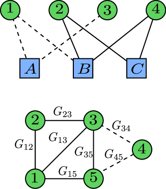
To investigate the local connectivity of nodes and examine the impact of highly-connected nodes, we calculate bipartite clustering coefficients martacluster ; Zhang20086869 . In bipartite networks, a clustering coefficient for a node can be calculated by counting the number of cycles of length 4 (i.e., the number of “squares”) that include the node and dividing the result by the total possible number of squares that could include the node. As stated by Zhang et al. in Zhang20086869 , the possible (or underlying) number of squares is calculated by adding the potential links (including existing ones) between a particular node and the neighbors of its neighbors. In Fig. 6 we show how a square occurs in a bipartite network when two neighbors of a node have another neighbor in common. Bipartite networks cannot have triangles (three mutually-connected nodes) because two nodes of the same type cannot be neighbors, so a square is the shortest possible cycle.

Figure 6: (Color online) Examples of how to calculate clustering coefficients for bipartite (top) and unipartite (bottom) networks. In the bipartite network, solid lines indicate edges that form the square that includes node $B$, whose bipartite clustering coefficient calculated according to equation (5) is $C_{4}=1/5$. One obtains this result because there are five possible squares for this node ({$1A2B$, $1C2B$, $1A4B$, $1C4B$, $2C4B$}) but only one of them ($2C4B$) actually exists. In the unipartite network, the solid lines indicate edges that form the triangles that include node $1$. If this were an unweighted network, for which $G_{ij}\in\{0,1\}$ for all $i$ and $j$, then one would obtain an unweighted clustering coefficient of $C_{3}(1)=2/3$. To calculate the value of its weighted clustering coefficient $\tilde{C}_{3}$, we use equation (6).

The definition of a clustering coefficient of node $m_{i}$ in an unweighted bipartite network is Zhang20086869 :

$$C_{4}(m_{i})=\frac{\sum_{h,j}{q_{i_{jh}}}}{\sum_{j,h}{\left[(k_{j}-\eta_{i_{jh}})+(k_{h}-\eta_{i_{jh}})+q_{i_{jh}}\right]}}\,,$$ (5)

where $q_{i_{jh}}$ is the observed number of squares containing $m_{i}$ and any two neighbors $u_{h}$ and $u_{j}$. The degrees of the neighbors are $k_{h}$ and $k_{j}$, respectively, and $\eta_{i_{jh}}=q_{i_{jh}}+1$. The possible number of squares is calculated adding the degrees of the nodes $u_{h}$ and $u_{j}$ minus the link that each shares with $m_{j}$ if the three nodes are not part of a square to avoid double-counting. If the three nodes are part of a square, then the square represented by the deleted link must be added again, hence $(k_{j}-\eta_{i_{jh}})+(k_{h}-\eta_{i_{jh}})+q_{i_{jh}}$ in the denominator of equation (5).

Figure 7: (Color online) Bipartite clustering coefficients $C_{4}(m_{i})$ for video (blue) and user nodes (inset, green) for August 12, 2003 (a Tuesday). The mean values for this day are $\langle C_{4}\rangle=\frac{1}{M}\sum_{i=1}^{M}C_{4}(m_{i})\approx 0.02606$ for the videos and $\langle C_{4}\rangle=\frac{1}{U}\sum_{i=1}^{U}C_{4}(u_{i})\approx 0.03144$ for the users.

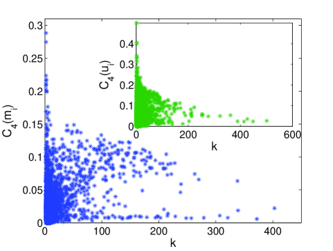
In Fig. 7, we show the values of $C_{4}(m_{i})$ for the video and user nodes for a single day (Tuesday, August 12, 2003). In Table 2, we show the mean values of the bipartite clustering coefficient of all one-day snapshots of Netflix in 2003. In spite of the weekday-dependent variation in the number of daily ratings, the values of the bipartite clustering coefficient do not vary significantly across weekdays. However, the values of $\langle C_{4}\rangle$ increase almost by 80% for both node-types on weekends. For a network constructed from a single day’s data, only about 2% of the possible squares typically exist; this is comparable to what would occur in a random network with the same degree distributions. To investigate whether the presence of blockbuster nodes (which have high degrees and increase considerably the number of possible squares) has any effect on the value of $\langle C_{4}\rangle$, we calculated the clustering coefficient after removing the top ten most rated videos. We did not find any conclusive evidence of blockbusters driving the value of the clustering coefficient; some of them caused the value of $\langle C_{4}\rangle$ to go down and others caused it to go up.

One can also examine clustering coefficients in the weighted unipartite networks given by the projected adjacency matrices $\mathbf{G}_{\mathcal{U}}$ and $\mathbf{G}_{\mathcal{M}}$. We calculate the weighted clustering coefficient for each projection using the formula PhysRevE.71.065103

$$\tilde{C}_{3}(m_{i})=\frac{2}{k_{i}(k_{i}-1)}\left[\frac{1}{G_{M}}\sum_{j,h}\left(G_{ij}G_{ih}G_{hj}\right)^{1/3}\right]\,,$$ (6)

where $k_{i}$ is again the degree of node $m_{i}$, $G_{ij}$ is the weight of the edge between $m_{i}$ and $m_{j}$, and $G_{M}=\max(G_{ij})$ denotes the maximum edge weight in the network. The geometric mean $(G_{ij}G_{ih}G_{hj})^{1/3}$ of the edge weights give the “intensity” of the $(i,j,h)$-triangle. When the network is unweighted, $(G_{ij}G_{ih}G_{hj})^{1/3}$ is $1$ if and only if all edges in the $(i,j,h)$-triangle exist and $0$ if they do not, reducing the equation to the unweighted unipartite clustering coefficient

$$C_{3}(m_{i})=\frac{2t_{i}}{k_{i}(k_{i}-1)}\,,$$ (7)

where $t_{i}$ is the number of triangles that include node $m_{i}$.

Figure 8: Weighted clustering coefficient $\tilde{C}_{3}(u_{i})$ for nodes in the unipartite projection onto users for August 4, 2003. The $x$-axis represents node degrees, and the $y$-axis represents $\tilde{C}_{3}(u_{i})$. The mean values for this day are $\langle\tilde{C}_{3}\rangle=\frac{1}{U}\sum_{i=1}^{U}\tilde{C}_{3}(u_{i})\approx 0.0013$ for the projection onto users and $\tilde{C}_{3}\approx 0.0086$ for the projection onto videos (not shown). The inset shows values of the unweighted coefficient $C_{3}(u_{i})$ from the same data.

$\langle C_{4}\rangle$ $\langle\tilde{C}_{3}\rangle$ mean var mean var Videos 0.02039 0.0007 0.0056 $10^{-6}$ Users 0.02092 0.0012 0.0044 $10^{-6}$

Table 2: Means and variances of $\langle C_{4}\rangle$ (for the bipartite network) and $\langle\tilde{C}3\rangle$ (for the projections) of videos and users on single-day snapshots of 2003, calculated using equations (5) and (6).

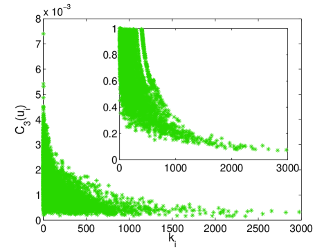
In Fig. 8, we show the $\tilde{C}_{3}(u_{i})$ values for the user projection $\mathbf{G}_{\mathcal{U}}$ (with 10,228 nodes and 814,667 edges) from Tuesday, August 4, 2003. In Table 2, we show the mean clustering-coefficient values for the projected user and video networks for all single-day snapshots of 2003. The values of $\langle\tilde{C}3\rangle$ did not vary much among weekdays, except for the videos’ $\langle\tilde{C}3\rangle$ that almost doubled its value on the weekends from an average of 0.0045 from Monday to Friday to 0.0086 on Saturday and Sunday.

Given the values of $\langle C_{4}\rangle$ in Table 2, it is unsurprising that the values of $\langle\tilde{C}_{3}\rangle$ are also typically low. In the inset of Fig. 8, we show the values of the users’ unweighted clustering coefficient $C_{3}$, which are naturally much higher. For example, about 4000 users have $C_{3}=1.0$, indicating that all potential triangles exist among these users. This differentiates one set of nodes from the rest. This feature, which we observe often in the data, arises from the dominant video of the day. For August 4, 2003, this video (which is typically a blockbuster) was Daredevil, which had 396 ratings and created many edges in the user projection among the users who rated it. Removing Daredevil from the bipartite network also removes these deviant nodes. This feature is not apparent if one calculates only the unweighted unipartite clustering coefficient ${C}_{3}$. Just as we did with $\langle C_{4}\rangle$, and given the dramatic effect observed by removing Daredevil, we calculated $\langle C_{4}\rangle$ for the projected network of users removing the ten most rated videos. We found that for every additional video removed, the value of $\langle C_{3}\rangle$ increased by 0.2%, while for $\langle\tilde{C}_{3}\rangle$ the increment was slightly larger.

III User Bursts

Figure 9: (Color online) Cumulative distribution of the inter-event time between the ratings of one Netflix user. The user signed up on April 4, 2000, and has a degree of 940 based on ratings cast over a period of almost five years. The dashed curve indicates the fit to the function $F(x)\sim x^{-\alpha}$, which yields $\alpha\approx 2.27$ in this case. The inset shows the number of days between consecutive video ratings.

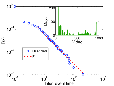
A close examination of the rating habits of individual users can also yield rich and informative insights. Recent research has shown that people tend to have bursts of e-mail and postal correspondence, in which they send and receive numerous messages within short periods of time, followed by long periods of inactivity barabasi-2005-435 ; oliveira2005437 ; burstbook . We find similar features in the Netflix data, as about 70% of the users exhibit bursty behavior by rating several videos in one go after several days of no activity. We illustrate this phenomenon in Fig. 9 by plotting the cumulative distribution of inter-event times between the ratings of one user over a period of almost five years. We fit this distribution to a power law $F(x)\sim x^{-\alpha}$ using the method discussed in Ref. Clauset:2007p5520 to determine the value of the exponent $\alpha$. We can similarly provide estimates for possible power laws (with actual power laws over roughly two decades of data) among the other bursty users, though the value of $\alpha$ depends on the final degree (i.e., the total number of rated videos) of the user. For example, bursty users with final degrees between 100 and 1000 have a mean exponent of $\alpha\approx 2.54$, whereas those with final degrees of at least 4000 have a mean exponent of $\alpha\approx 3.17$. Additionally, there are several types of users among those who do not exhibit bursty dynamics. In particular, some users rated only a very small number of videos (which may be due to the sampling done by Netflix) and others exhibit seemingly unrealistic levels of rating activity. (For example, there are 47 users who signed up in January 2004 or later and who have rated more than 4000 videos each.)

IV Catalog Networks

The above empirical investigation of the Netflix data motivates the development of an evolution model for bipartite catalog networks, which arise in a diverse set of applications. Such networks have two sets of nodes whose numbers can be fixed or dynamic, and edges are placed one at a time between previously unconnected edges that are chosen according to predefined rules. One continues to add edges until a predefined final time has been reached or the system has become saturated, at which point every node in one partite set is connected to every node in the other partite set. The Netflix network can be studied using such a catalog network framework; it starts completely disconnected (nobody has rated any videos), and the users start choosing and rating videos from the catalog. Depending on the way the data set is sampled, the catalogs can be static (e.g. a one-day snapshot) or dynamic (e.g. the full data set). Catalog models of network evolution are closely related to the network rewiring problem studied by Plato and Evans evans:056101 ; evans-2008-3 that features fixed sets of artifacts and individuals. Every individual has one affiliation (a connection) with an artifact and can reassign this connection to another node as the network evolves. In contrast, in a catalog network, any edge that has been placed between two nodes in the network is permanent. Consequently, catalog networks are suited to describing records of interactions that are assigned dynamically and then remain permanently in the system.

As before, $\mathcal{U}$ denotes the set of users and $\mathcal{M}$ denotes the set of videos. The size of $\mathcal{U}$ is $u(r)$ and the size of $\mathcal{M}$ is $m(r)$, where $r$ denotes a discrete time that is indexed by the ratings. That is, we take every rating event as a time step, so when we discuss time in this context, we are referring to “rating time” and not physical time unless we indicate otherwise. Because $m(r)$ and $u(r)$ are not always integers, we define $U(r)=\left\lfloor u(r)\right\rfloor$ and $M(r)=\left\lfloor m(r)\right\rfloor$ as the (nonnegative integer) numbers of user and video nodes, respectively. The associated time-dependent catalog vectors, $D_{\mathcal{U}}$ and $D_{\mathcal{M}}$, have components given by the degrees of each node in the catalog:

$$D_{\mathcal{U}}(r)=\begin{bmatrix}k_{u_{1}}(r)\\ k_{u_{2}}(r)\\ \vdots\\ k_{u_{U}(r)}(r)\end{bmatrix},\qquad D_{\mathcal{M}}(r)=\begin{bmatrix}k_{m_{1}}(r)\\ k_{m_{2}}(r)\\ \vdots\\ k_{m_{M}(r)}(r)\end{bmatrix}\,.$$ (8)

These vectors have size $U(r)$ and $M(r)$, respectively. We denote by $N_{\mathcal{U}}(r,k)$ (with $k\in\{0,1,\ldots,M(r)\}$) and $N_{\mathcal{M}}(r,k)$ (with $k\in\{0,1,\ldots,U(r)\}$) the numbers of users and videos, respectively, that have degree $k$ at rating time $r$. One can normalize $N_{\mathcal{U}}(r,k)$ to obtain the proportion of nodes with degree $k$ given by $\hat{N}_{\mathcal{U}}(r,k)=\frac{1}{U(r)}N_{\mathcal{U}}(r,k)$. An analogous relation holds for $\hat{N}_{\mathcal{M}}(r,k)$.

Based on our intuition about the choosing and rating of videos, we add edges to the network using a combination of linear preferential attachment and uniform attachment. On one hand, one expects the choice of a user to be driven in part by the choices made by others, as popular videos are more likely to attract further viewings and hence ratings. On the other hand, one also expects an element of idiosyncrasy on the part of each user, allowing him or her to choose any video from the catalog regardless of the choices of others. This results in two time-dependent probabilities—one for users and one for videos—each of which consists of a convex combination of preferential and uniform attachment. More specifically, each time an edge is added to the network, we select a user and a video to be connected by this new edge. The video (user) node is chosen using uniform attachment with probability $1-q$ (respectively, $1-p$) and linear preferential attachment with probability $q$ (respectively, $p$). The addition of an edge occurs during a single discrete (rating) time step, as is common in models of network evolution. Combining these ideas, a video node with degree $k_{i}$ is chosen with probability

$$P_{\mathcal{M}}(r,k_{i}) =\frac{1-q}{M(r)-N_{\mathcal{M}}(r,U(r))}$$

$$\quad+\frac{qk_{i}}{\|D_{\mathcal{M}}(r)\|_{1}-U(r)N_{\mathcal{M}}(r,U(r))}\,,$$ (9)

and a user node with degree $h_{i}$ is chosen with probability

$$P_{\mathcal{U}}(r,h_{i}) =\frac{1-p}{U(r)-N_{\mathcal{U}}(r,M(r))}$$

$$\quad+\frac{ph_{i}}{\|D_{\mathcal{U}}(r)\|_{1}-M(r)N_{\mathcal{U}}(r,M(r))}\,,$$ (10)

where the values of the parameters $p,q\in[0,1]$ are fixed, $\|D_{\mathcal{U}}(r)\|_{1}=\sum_{i=1}^{U(r)}k_{i}(r)$, and $\|D_{\mathcal{M}}(r)\|_{1}=\sum_{i=1}^{M(r)}h_{i}(r)$. The probabilities $P_{\mathcal{U}}(r,h_{i})$ and $P_{\mathcal{M}}(r,k_{i})$ change over time as the degrees of the nodes change when edges are added to the network.

The denominators in equations (9-10) contain the terms $N_{\mathcal{M}}(r,U(r))$ and $N_{\mathcal{U}}(r,M(r))$ because once a node of either type is fully connected, it is no longer eligible to receive any new connections and is effectively no longer in the catalog until a new node of the other type arrives. When $r=0$, one obtains $\|D_{m}(0)\|_{1}=\|D_{u}(0)\|_{1}=0$ and $N_{\mathcal{M}}(0,U(r))=N_{\mathcal{U}}(0,M(r))=0$, which would result in division by zero. To overcome this problem, we follow the standard procedure employed in network growth models albert-2002-74 by seeding the algorithm with an edge that connects two randomly-chosen nodes (one from each of the partite sets). This is equivalent to shifting the rating-time variable and changing the initial conditions to $\|D_{m}(0)\|_{1}=\|D_{u}(0)\|_{1}=1$.

IV.1 Rate Equations

One can use rate equations (i.e., master equations) to investigate the dynamics of the degree distributions of a catalog network. This type of approach has been used successfully to study a variety of other networks PhysRevLett.85.4629 ; evans:056101 ; evans-2008-3 ; PhysRevLett.86.3200 ; PhysRevE.71.036127 ; Newman:2003 . The analysis of the degree distribution for videos in the catalog model is identical to the one for users, as only the constants and sizes of the catalogs are different. Accordingly, we present our results for the degree distributions of the videos; one obtains the results for user distributions by changing $q$ to $p$, $M(r)$ to $U(r)$, and $P_{\mathcal{M}}(r,k)$ to $P_{\mathcal{U}}(r,k)$. For notational convenience, we also drop the subscripts in this subsection, so $N(r,k)$ denotes the number of nodes with degree $k$ at time $r$. To construct the rate equations, one must consider how many nodes pass through $N(r,k)$ (i.e. turn into nodes of degree $k$ and $k+1$) for $k\in\{0,1,2,\ldots,U(r)\}$. This yields

$$\frac{\mathrm{d}N(r,0)}{\mathrm{d}r} =m^{\prime}(r)-P_{\mathcal{M}}(r,0)N(r,0)\,,$$

$$\frac{\mathrm{d}N(r,k)}{\mathrm{d}r} =P_{\mathcal{M}}(r,k-1)N(r,k-1)$$ (11)

$$-P_{\mathcal{M}}(r,k)N(r,k)\,,\quad k>0,$$

where $m^{\prime}(r)=\frac{\mathrm{d}m(r)}{\mathrm{d}r}$. The initial conditions are

$$N(0,0) =M(0)-1\,,$$

$$N(0,1) =1\,,$$ (12)

$$N(0,k) =0\,,\quad k>1\,.$$

Equation (11) is a system of coupled nonlinear ordinary differential equations (ODEs). The positive and negative terms account, respectively, for an increase and decrease in the number of nodes of a given degree as nodes receive new edges. The equation for $N(r,0)$ has $m^{\prime}(r)$ as a positive term to indicate the entry of new nodes (with degree $0$) to the network. The time-dependent probabilities $P_{\mathcal{M}}(r,k)$ are defined in equation (9). In the case of fixed catalogs, there is a maximum value of $k$, so the final equation in (11) takes a slightly different form (see below).

IV.1.1 Fixed Catalogs

We begin by analyzing the evolution of the network with fixed catalog sizes, so $U(r)=U$, $M(r)=M$, and $m^{\prime}(r)=0$ for all $r$. Because a finite, fixed number of users and videos are available in the catalogs, the network can only evolve until time $r=UM$. At this point, the system becomes saturated (i.e., $N_{\mathcal{U}}(MU,M)=U$ and $N_{\mathcal{M}}(MU,U)=M$), and no additional edges can be added to the network. Note additionally that the equations in (11) change slightly for fixed catalogs. In particular, the last equation for nodes with degree $U$ changes to

$$\frac{\mathrm{d}N(r,U)}{\mathrm{d}r}=P_{\mathcal{M}}(r,U-1)N(r,U-1)\,,$$ (13)

which only has one positive term because nodes with degree $U$ stay that way until the end of the process.

Additionally, while the degree distribution of a network generated using the catalog model with static node sets is time-dependent, the long-time asymptotic behavior is always the same:

$$\lim_{r\to UM}N(r,k)=\left\{\begin{array}[]{lll}M\,,&\mathrm{if}&k=U\,,\\ 0\,,&\mathrm{if}&k<U\,,\end{array}\right.$$

which gives a de facto final condition to the system in (11-13). Accordingly, we examine degree distributions for $r\leq UM-1$.

Figure 10: (Color online) Degree distributions of video nodes averaged over 500 simulations of a fixed catalog network with $U=100$ users, $M=30$ videos, and $q=0.8$ at rating times $r=500$ (red diamonds) and $r=1000$ (blue squares). The solid curves are the solutions to the differential equation (11).

Figure 11: (Color online) Numbers of nodes $N(r,0)$ with degree $0$ (red triangles) and $N(r,100)$ (blue circles) with degree $100$ from 500 simulations of a fixed catalog network with $U=100$, $M=30$, and $p=0.8$. Inset: Decrease of $N(t,0)$ on a semi-logarithmic scale, which appears to decrease exponentially. The solid curves come from the solutions of (11).

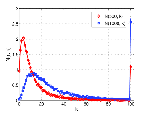
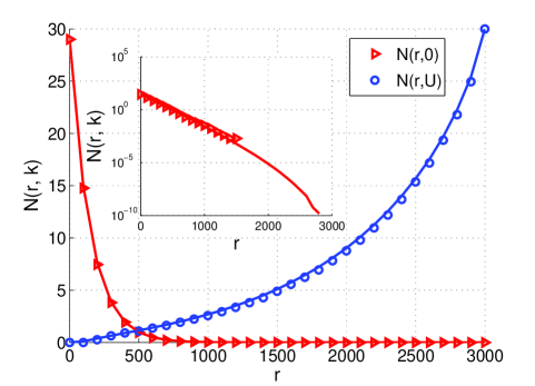
In Fig. 10, we show the degree distribution of the video nodes averaged over 500 simulations of a fixed catalog network with $U=100$ and $M=30$ at different times during its evolution. As the discrete time $r$ increases, the peaks of the functions travels towards higher values of $k$ and decrease as if they were diffusing. We also observe a jump in $N(r,k)$ at $k=U$. This occurs because there are nodes in the network that become fully connected during the edge-assignment process (see Fig. 11). Interestingly, Johnson et al. showed recently that the time-dependent degree distributions observed in some networks that undergo edge rewiring with preferential attachment follow nonlinear diffusion processes PhysRevE.79.050104 .

Figure 12: (Color online) Mean of $N(r,k)$ for user nodes in 500 simulations of a fixed catalog network with $U=100$, $M=30$, and $p=0.5$. The axes are (rating) time $r$ and degree $k$, and the color indicates the value of $\log(N(r,k)+1)$. The horizontal line at the top of the image is the discontinuity (as seen with the video nodes in Fig. 11) that corresponds to the value of $N(r,M)$ and reflects the appearance of fully-connected user nodes.

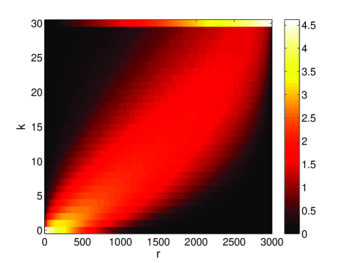
Figure 12 reveals how the user nodes achieve full connectivity between $r=0$ and $r=UM-1$. The image shows the “paths” that user nodes follow in the $(r,k)$-plane between $(0,0)$ and $(UM-1,M)$. For example, the nodes that follow a steep (high $k$ for early $r$) trajectory are the ones that receive many links early on. Their degree grows mostly from preferential attachment in the edge-assignment mechanism, and they accordingly achieve full connectivity early in the process. The nodes that acquire edges more slowly initially begin to receive edges very fast as $r$ approaches $UM$ (because other nodes have already saturated), explaining the steep climb in the upper right corner of the figure.

Figure 13: (Color online) Numerical solution of $N(r,k)$ for video nodes from equation (11) with a fixed catalog and $q=0.8$, $M=30$, and $U=100$. (We again plot $\log(N(r,k)+1)$.) The horizontal line at $k=100$ corresponds to the saturated nodes $N(r,U)$. The inset shows a plot of $N(r,U-1)$ for the same network.

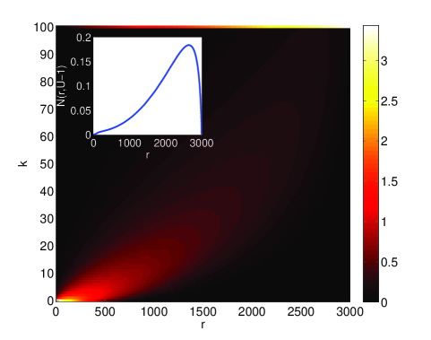
The “final” condition that $N(UM-1,U)=M$ makes the system in (11) very stiff for high values of $k$ and $r$. Fig. 13 shows the path that the video nodes follow in the $(r,k)$-plane (i.e., the same information as in Fig. 12 but for video nodes) but for the numerical solutions of (11) instead of direct network simulations. In the inset of the Fig. , we show the profile of $N(r,U-1)$ which evinces the aforementioned stiffness. Because all nodes must be fully connected at $r=UM-1$, nodes with low degrees begin to receive many edges for high values of $r$. This causes $N(r,k)$ for high $k$ to peak late in the process, and the nodes “travel” through values of $k$ rather quickly, which explains the incredibly steep slope of $N(r,U-1)$ as $r$ approaches $UM-1$.

The value of $q$ affects the width of the region (light colored) in the $(r,k)$ plane. For lower values of $q$ (e.g., $q=0.3$), uniform random attachment dominates and the region of activity becomes narrower. The nodes attain edges at roughly the same pace. For larger values of $q$, the first nodes to receive edges become more likely to continue receiving more nodes until they saturate, and the area of activity of the nodes becomes wider (see Fig. 13).

IV.1.2 Growing Catalogs

In the previous section, we described the dynamics of catalog networks when the sizes of the catalogs are fixed. While this provides a good baseline investigation, catalogs can grow in many applications—for example, Netflix gains both new subscribers and new videos almost every day. Accordingly, in this section we study the dynamics of (11) for growing catalogs for which $m^{\prime}(r)>0$.

Figure 14: (Color online) Numerical solution of $N(r,k)$ for video nodes from equation (11) with $q=0.8$, $m(r)=30+0.007r$, and $U=100+0.05r$. (We again plot $\log(N(r,k)+1)$.) The increasing diagonal line gives $U(r)$ and represents the temporarily saturated nodes. In the inset, we show a plot of $N(r,0)$ on a semilogarithmic scale. We observe a rapid initial decrease followed by a slower increase as the catalog grows.

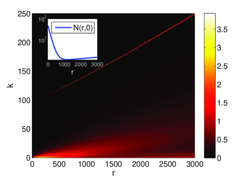
The system no longer has an obligatory final time, and the saturation level of nodes is now time-dependent. For example, a user that has degree $M(r)$ is saturated temporarily until a new video “arrives”—i.e., until time $r+\Delta r$ so that $M(r+\Delta r)-M(r)>0$ and there is a new video to rate.

In Fig. 14, we show a numerical solution to equation (11) where $m(r)$ and $u(r)$ are linear functions of $r$. Instead of the horizontal line of fully connected nodes along $k=100$ in Fig. 13, the saturation of the nodes follows the growth of $U(r)$. In the inset of Fig. 14, we show the time profile of $N(r,0)$. Initially, it has what appears to be exponential descent before it starts to grow slowly as the catalog size increases, in contrast to what we observed in Fig. 11. The early rapid decay is explained by the absence of many nodes with high degrees, so nodes with lower degrees receive edges. As $r$ increases, the better-connected nodes receive more edges (because for $q=0.8$ the dominant mechanism is linear preferential attachment) and the population of nodes with fewer edges increases slowly. In Section V, we discuss how the Netflix data displays some of these features.

V Netflix as a Catalog Network

We now investigate how well our catalog model captures the human dynamics revealed by the Netflix data. To do this, we sample the data set while keeping in mind the following considerations:

• Because of the way we have defined our catalog network growth model, we must consider the evolution of the Netflix data in “rating time”, in which every new rating (which adds an edge in the network) constitutes a time step.

• Although there might be a (physical) time difference between a node (either user or video) joining Netflix and the node receiving its first edge, this information is not included in the data. Many videos receive more than one rating on their first day, so their entry to the network is reflected by increases in the value of $N(r,k)$ for several values of $k$. We will have to take this into account when comparing our model to the data.

V.1 Growth and Dynamics

To compare our results to the data, we express the growth of the numbers of videos and users as a function of rating time $r$. Solving for $t$ in equation (1) gives

$$t=\frac{1}{b_{r}}\log{\left(\frac{r}{a_{r}}+1\right)}\,.$$ (14)

We substitute (14) into (2) to obtain the new expressionfor the users as a function of ratings:

$$u(r)=a_{u}\left[\left(\frac{r}{a_{r}}+1\right)^{b_{u}/b_{r}}-1\right]\,.$$ (15)

We follow the same procedure for the videos to obtain

$$m(r)=a_{m}+b_{m}\left\{\frac{1}{b_{r}}\log{\left(\frac{r}{a_{r}}+1\right)}\right\}^{c_{m}}\,.$$ (16)

Figure 15: (Color online) Users (top) and videos (bottom) as a function of ratings. We use circles to show the data from Netflix and dashed curves to show the predictions from equations (15) and (16). We use the parameter values obtained in Sec. II.

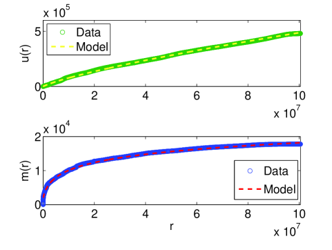
In Fig. 15, we show the numbers of users and videos versus the number of ratings in the network. Observe that the predictions from equations (15-16) agree very well with the data.

Figure 16: (Color online) Video degree distribution $N_{\mathrm{data}}(r,k)$ in the Netflix data set in 2000. (We again plot $\log(N_{\mathrm{data}}(r,k)+1)$.) We show data for videos with degrees ranging from 1 to 4794.

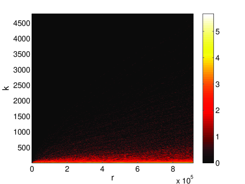
Figure 16 shows the time-dependent degree distribution of videos in the Netflix data set for the year 2000. The sample in the plot consists of 365 measurements (one for each day) of $r$ and $N(r,k)$. The highest degree in this sample is 4794; this is well below the theoretical maximum of 9289 according to the expression for $u(r)$ in equation (15), so the network is not experiencing node saturation. We can rewrite the probability that a video node receives an edge as

$$P_{\mathcal{M}}(r,k_{i})=\frac{1-q}{M(r)}+\frac{qk_{i}}{\|D_{\mathcal{M}}(r)\|_{1}}\,.$$

The rate equation for the evolution of the degree distribution is

$$\frac{\mathrm{d}N(r,1)}{\mathrm{d}r}= \delta_{1}m^{\prime}(r)-P_{\mathcal{M}}(r,1)N(r,1)\,,$$

$$\frac{\mathrm{d}N(r,k)}{\mathrm{d}r}= \delta_{k}m^{\prime}(r)+P_{\mathcal{M}}(r,k-1)N(r,k-1)$$ (17)

$$\quad-P_{\mathcal{M}}(r,k)N(r,k),\quad k>1.$$

The initial conditions are $N(0,1)=m(0)$ and $N(0,k)=0$ for $k>1$. As noted earlier, the lowest degree a node can have in the data is $1$ and the entry degree of the nodes can have any value of $k$. We denote by $\delta_{k}$ the proportion of new nodes whose entry degree is $k$, such that $\sum_{k}\delta_{k}=1$. We investigated how many ratings do videos receive on the day that they entered the system and found that over $97\%$ of the new nodes receive $3$ or fewer ratings. Consequently, we have set $\delta_{1}=0.8$, $\delta_{2}=0.15$, and $\delta_{3}=0.05$.

To see how well our model describes the Netflix video data in the year 2000, we define $N_{k}(q)$ as the $4794\times 365$ matrix obtained solving the system in (17) and $N_{\mathrm{data}}$ obtained from the data sample. These two matrices contain the values of $N(r,k)$ from the sample and from the equations for all values of $k$ and $r$. The matrices are of the given size because we sample the degree distribution once per day and the maximum degree observed is 4794. We define the error function

$$E(q)=\|N_{k}(q)-N_{\mathrm{data}}\|\,,$$ (18)

where $\|\cdot\|$ is the Euclidean matrix norm. To find the optimum value $q^{*}$, we minimize $E(q)$ using the Nelder-Mead derivative-free simplex method lagarias:112 . We found that the value of $q$ that minimizes (18) is $q^{*}\approx 0.9795$, meaning that according to the model about $98\%$ of the decisions to rate a video by users are guided by its popularity (i.e., preferential attachment).

Figure 17: (Color online) Values of $N(r,10)$ (videos with degree 10) obtained by solving (17) using $q=0.9795$ (red curve) and the data from Netflix that we report in Fig. 16 (blue dots).

Figure 18: (Color online) Values of $N(r,50)$ (videos with degree 50) obtained by solving (17) using $q=0.9795$ (red curve) and the data from Netflix that we report in Fig. 16 (blue dots).

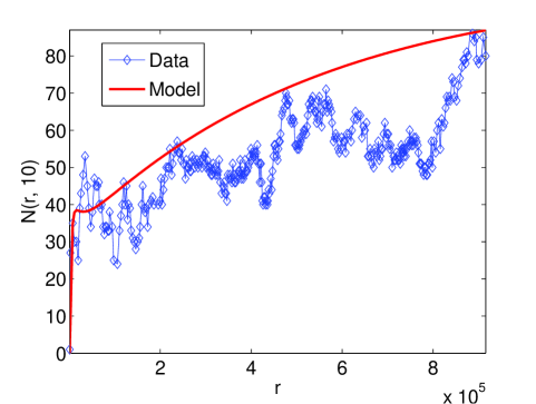
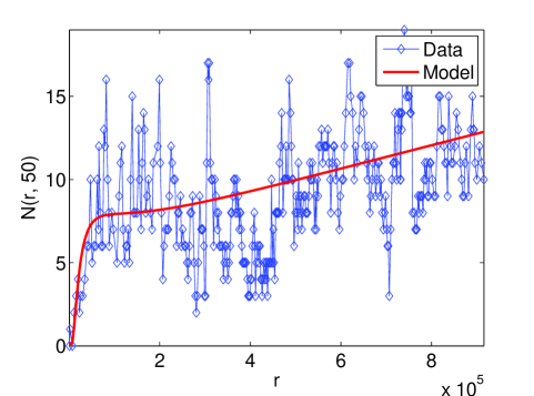
In Figs. 17 and 18, we compare the values of $N(r,k)$ that we obtained in our model to those in the data. In spite of the noise in the data, our model is able to reproduce the temporal dynamics of $N(r,k)$.

Figure 19: (Color online) Cumulative degree distribution of video nodes on the last day (915628 ratings) of the sample from year 2000. We obtained this by solving (17) using $q=0.9795$ (red curve) and directly from the data (blue dots).

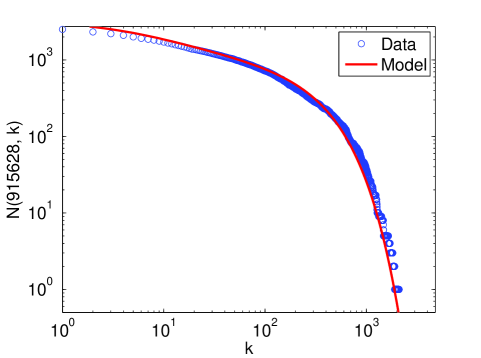
In Fig. 19, we show the approximation of our model to the cumulative degree distribution of the videos on the last day of the sample (i.e., for all values of $k$ and $r=915628$, the number of ratings at the end of year 2000), which agrees very well with the data.

Although $q^{*}\approx 0.9795$ suggests that the way the users choose to rate videos is dominated by the popularity of the films, we should stress that the model developed here is a very simple one. There are probably many other processes influencing the decisions of the users, including different external (to the user) factors, such as advertisements, press, and the underlying social network the users are embedded in.

VI Conclusions

We have analyzed a large network of video ratings given by the users of the Netflix video rental service. We studied the system using a bipartite network of videos and users and employed this perspective to reveal interesting features in the dynamics of video rating, such as weekly patterns in video ratings and bursts of activity followed by long idle periods. We calculated clustering coefficients for one-day snapshots, concluding that their low values arise from the presence of high-degree nodes (i.e., videos with a large number of ratings and users who rate many videos). We also showed that the degree distributions of both the user and video nodes resemble power laws with exponential cutoffs.

Motivated by the structural and dynamical features we observed in the Netflix data, we formulated a mechanism of network evolution in the form of “catalog networks” for bipartite systems. Such networks are initially empty (aside from a seed), and edges are created between two types of nodes based on some predefined rules. New nodes can also be added to the network during the wiring process. In our model, we considered a combination of uniform random attachment and linear preferential attachment. We derived a set of coupled ordinary differential equations that describe the time-evolution of the degree distributions of such catalog networks. Presupposing this mechanism and employing the Netflix data, we found that users seem to choose videos according to preferential attachment about 98% of the time and uniform attachment about 2% of the time. This suggests that the number of ratings for a given video is driven almost completely by its popularity (preferential attachment) and only in very small measure by the intrinsic preferences of users. While interesting, the extreme dominance of a preferential-attachment mechanism might be due in part to the simplicity of our model and the absence of information about the underlying social network of the users, which can have considerable influence over the video choices.Additionally, our model does not incorporate external influences such as media coverage and promotion campaigns that can certainly affect the popularity of videos. One can refine such insights by considering more sophisticated attachment mechanisms that incorporate the actual scores of the video ratings (not just their existence), the age of the videos, user social networks (see Refs. Asur2010 and Ratkiewicz2010 for recent interesting study), interactions among users, media presence of videos, and more. Our simple catalog model thereby serves as a good starting point for an abundance of interesting generalizations.

The Netflix data, which is both large and publicly available, provides an excellent vehicle to study many of the features that have been observed in network representations of systems in which agents exercise preferences or choices, such as citation, collaboration, and social networks Price:1965 ; albert-2002-74 ; Sornette.93.228701 ; Salganik02102006 ; Lambiotte2005 ; oliveira2005437 . In this paper, we formulated a catalog model to understand the human dynamics of video rating. In our view, catalog models are suitable in many other contexts, including studying certain electoral systems (such as the preamble to preferential voting elections) AustralianPolitics.com , professional sports drafts HockeyDraft , and retail shopping. To achieve insights in such a diverse array of settings, the catalog model presented herein can be generalized in numerous interesting ways to incorporate external agents, underlying networks or cliques of individuals, and more.

References

- (1) A.-L. Barabasi, Nature 435, 207 (2005).
- (2) T. S. Evans and A. D. K. Plato, Networks and Heterogeneous Media 3, 221 (2008).
- (3) J.-P. Onnela et al., Proceedings of the National Academy of Sciences 104, 7332 (2007).
- (4) R. Albert and A.-L. Barabási, Reviews of Modern Physics 74, 47 (2002).
- (5) M. E. J. Newman, SIAM Review 45, 167 (2003).
- (6) M. E. J. Newman, Proceedings of the National Academy of Sciences 98, 404 (2001)
- (7) G. Calderelli, Scale-Free Networks, Oxford University Press, 2007.
- (8) J. L. Gross and J. Yellen, editors, Handbook of Graph Theory, CRC Press, 2004.
- (9) A.-L. Barabási and R. Albert, Science 286, 509 (1999).
- (10) H. A. Simon, Biometrika 42, 425 (1955).
- (11) D. J. d. S. Price, Science 149, 510 (1965).
- (12) P. L. Krapivsky, S. Redner, and F. Leyvraz, Physical Review Letters 85, 4629 (2000).
- (13) M. Latapy, C. Magnien, and N. D. Vecchio, Social Networks 30, 31 (2008).
- (14) M. A. Porter, P. J. Mucha, M. E. J. Newman, and C. M. Warmbrand, Proceedings of the National Academy of Sciences 102, 7057 (2005).
- (15) S. Saavedra, F. Reed-Tsochas, and B. Uzzi, Nature 457, 463 (2009).
- (16) P. Zhang et al., Physica A 387, 6869 (2008).
- (17) J.-L. Guillaume and M. Latapy, Bipartite graphs as models of complex networks, in Aspects of Networking, pages 127–139, Springer, 2004.
- (18) J. Ohkubo, K. Tanaka, and T. Horiguchi, Physical Review E 72, 036120 (2005).
- (19) T. S. Evans and A. D. K. Plato, Physical Review E 75, 056101 (2007).
- (20) S. Saavedra et al., Physica A 389, 1131 (2010).
- (21) G. F. Davis, M. Yoo, and W. E. Baker, Strategic Organization 1, 301 (2003).
- (22) D. J. Watts and S. H. Strogatz, Nature 393, 440 (1998).
- (23) S. N. Dorogovtsev, J. F. F. Mendes, and A. N. Samukhin, Nuclear Physics B 666, 396 (2003).
- (24) K. Park, Y.-C. Lai, and N. Ye, Physical Review E 72, 026131 (2005).
- (25) H. Fan, Z. Wang, T. Ohnishi, H. Saito, and K. Aihara, Physical Review E 78, 026103 (2008).
- (26) J. Lindquist, J. Ma, P. van den Driessche, and F. H. Willeboordse, Physica D 238, 370 (2009).
- (27) G. Polya, Annalea de 1’Institut Henri Poincaré 1, 117 (1931).
- (28) W. Feller, An Introduction to Probability Theory and Its Applications, Vol. 1, John Wiley & Sons, Inc., 1957.
- (29) C. Godrèche and J. M. Luck, Journal of Physics: Condensed Matter 14, 1601 (2002).
- (30) D. Stauffer, X. Castelló, V. M. Eguíluz, and M. S. Miguel, Physica A 374, 835 (2007).
- (31) R. A. Bentley and S. J. Shennan, American Antiquity 68, 459 (2003).
- (32) Netflix-Prize, http://www.netflixprize.com.
- (33) J. Lorenz, European Physical Journal B 71, 251 (2009).
- (34) J. Bennett and S. Lanning, Proceedings of KDD Cup and Workshop 2007 (2007).
- (35) M. C. González, C. A. Hidalgo, and A.-L. Barabási, Nature 453, 779 (2008).
- (36) D. Sornette, F. Deschâtres, T. Gilbert, and Y. Ageon, Physical Review Letters 93, 228701 (2004).
- (37) J. G. Oliveira and A.-L. Barabási, Nature 437, 1251 (2005).
- (38) A.-L. Barabási, Bursts: The Hidden Pattern Behind Everything We Do, Dutton Adult, 2010.
- (39) A. Clauset, C. R. Shalizi, and M. E. J. Newman, SIAM Review 51, 661 (2009).
- (40) P. G. Lind, M. C. González, and H. J. Herrmann, Physical Review E 72, 056127 (2005).
- (41) J.-P. Onnela, J. Saramäki, J. Kertész, and K. Kaski, Physical Review E 71, 065103 (2005).
- (42) australianpolitics.com, History & features of the australian electoral system, 2008, Consulted on Feb, 10, 2009.
- (43) R. Pastor-Satorras and A. Vespignani, Physical Review Letters 86, 3200 (2001).
- (44) A. Barrat and R. Pastor-Satorras, Physical Review E 71, 036127 (2005).
- (45) S. Johnson, J. J. Torres, and J. Marro, Physical Review E 79, 050104 (2009).
- (46) J. C. Lagarias, J. A. Reeds, M. H. Wright, and P. E. Wright, SIAM Journal on Optimization 9, 112 (1998).
- (47) S. Asur and B. A. Huberman, (2010), arXiv:1003.5699.
- (48) J. Ratkiewicz, F. Menczer, S. Fortunato, A. Flammini, and A. Vespignani, (2010), arXiv:1005.2704v1.
- (49) M. J. Salganik, P. S. Dodds, and D. J. Watts, Science 311, 854 (2006).
- (50) R. Lambiotte and M. Ausloos, Phys. Rev. E 72, 066107 (2005).
- (51) A. Summers, T. Swartz, and R. Lockhart, In Statistical Thinking in Sports, chapter 15. Optimal drafting in hockey pools, pages 249–262, Chapman & Hall/CRC, 2007.