Laboratoire de Physique Nucléaire et des Hautes Énergies
Strategies for precision measurements
of the charge asymmetry of the boson mass
at the LHC within the ATLAS experiment
by
Florent Fayette
presented to the
Université de Paris VI – Pierre et Marie Curie
for the degree of Docteur de l’Université Paris VI
. This Ph.D. thesis was supervised by Dr. Mieczysław Witold Krasny at the LPNHE institute in Paris and it was eventually submitted to the Université de Paris VI - Pierre et Marie Curie to obtain the degree of Docteur de l’Université Paris VI on January 2009 in front of a committee consisting of Prof. Michael Joyce (President of the committee), Prof. Stefan Tapprogge (Referee), Prof. Fabian Zomer (Referee), Dr. Thomas LeCompte, Dr. Gavin Salam and Dr. Mieczysław Witold Krasny.
Abstract
This thesis dissertation presents a prospect for a measurement of the charge asymmetry of the boson mass () at the LHC within the ATLAS experiment. This measurement is of primordial importance for the LHC experimental program, both as a direct test of the charge sign independent coupling of the bosons to the fermions and as a mandatory preliminary step towards the precision measurement of the charge averaged boson mass. This last pragmatic point can be understood since the LHC specific collisions will provide unprecedented kinematics for the positive and negative channels while the SPS and Tevatron collider produced and on the same footing. For that reason, the study of the asymmetries between and in Drell–Yan like processes (production of single decaying into leptons), studied to extract the properties of the boson, is described thoroughly in this document.
Then, the prospect for a measurement of at the LHC is addressed in a perspective intending to decrease as much as possible the systematic errors that will inevitably comes from the misunderstanding of both phenomenological and apparatus modeling. For that matter strategies have been devised specifically for the present measurement to display robustness with respect to the main uncertainties. These strategies consist of introducing new observables along with considering specific LHC running modes and configurations of the ATLAS tracker.
Eventually we show that the present (2009) precision can be improved at the LHC by a factor of and argue that such a precision is beyond the reach of the standard measurement and calibration methods imported to the LHC from the Tevatron program.
J’en ai plein le QCD.
Remerciements, podziekowania, acknowledgements, etc.
Mes premiers remerciements s’adressent à ceux qui ont œuvré pour que j’obtienne une bourse pour réaliser ma thèse au LPNHE, à savoir Anne-Marie Cazabat, Matteo Cacciari, Jean-Eudes Augustin, Philippe Schwemling et Mieczysław Witold Krasny mon directeur de thèse. En particulier je tiens à exprimer ma reconnaissance à Pascal Debu, Philippe Schwemling et Witold Krasny pour avoir dispensé avec parcimonie toutes injonctions pour rattraper ce léger retard que j’accusais ce qui m’aura permis de parachever ma thèse en toute quiétude. Enfin je tiens à remercier Stefan Tapprogge et Fabian Zomer pour avoir accepté d’en être les rapporteurs et pour avoir studieusement pris en considération mon travail pendant leurs vacances de Noël. Cette gratitude s’adresse par ailleurs aux autres membres du jury, Michael Joyce, Tom LeCompte, Gavin Salam et mon directeur.
Je remercie ce dernier, Mieczysław Witold Krasny, pour m’avoir offert l’opportunité de faire ma thèse avec lui et surtout pour avoir su composer, à la faveur de mes capacités et de mes aspirations, un sujet de thèse idoine à ma délicate personne. Par bien des aspects travailler sous sa direction sur le présent sujet fit largement honneur au travail de recherche tel que l’on peut se le figurer dans l’idéal. Ces remerciements ne sauraient rendre justice à ce que furent ces trois dernières années en sa compagnie si je ne devais mentionner sa sympathie, sa bienveillance et pour ne m’avoir jamais mis sous pression favorisant en cela le plaisir dans le travail à la production de résultats équivoques. Enfin l’originalité du personnage, à mi-chemin entre le diable de Tasmanie et le “road-runner”, son génie ainsi que son humour ont fait de cette collaboration une expérience unique.
Just like to fire there is water, or to vodka there is miód pitny to Witold Krasny there is Wiesław Płaczek. On many aspects I consider Wiesław Płaczek as my second supervisor for all of his helps which improved the quality of my work over these last years. I learned a lot from his rigor, his infallible skills in informatics and I am indebted for all the multiple times he helped me using the WINHAC Monte Carlo. Besides I always appreciated his zen attitude and I also do not forget that most of my stays in Kraków would not have been possibly that smooth if it had not been for his attentions and his hospitality. Za wszystko dziȩkujȩ Ci polski mistrzu Zen.
I am deeply grateful to Giorgos Stavropoulos whose help and support, while fighting with Athena, allowed me to reach my first concrete results in my thesis. His broad sympathy really made of this task an agreeable moment, which, in regard of what Athena is, stands as a huge compliment.
Jestem wdziȩczny Andrzejowi Siódmokowi. Indeed, Andrzej brought equilibrium to tackle the Krasny–Płaczek doublet which would have been hard to tame all by myself (especially the M.W.K. component), besides I am grateful to him for his sympathy and his hospitality in Kraków. I also do not forget Katarzyna Rejzner whose recent arrival in our team brought additional fun and more importantly allowed to decrease the amount of krasnic activity Andrzej and I used to deal with.
Je remercie les membres du groupe ATLAS du LPNHE pour leur accueil et plus précisément Frédéric Derue pour s’être montré toujours disponible pour m’aider lors de mes confrontations non-ASCII avec Athena ainsi qu’Emmanuel Busato dont les aides, même après son départ pour Clermont–Ferrand, auront grandemement contribuer à améliorer la qualité de mon code. Je tiens aussi à rendre hommage à Emmanuel “Mini Manu” Hornero, Jérôme “Jers” Glisse et Rui Pereira pour avoir toujours pris le temps de s’intéresser aux problèmes informatiques sur lesquels je butais. Je double mes louanges à l’endroit de Rui et Jers dont les aides en Matplotlib auront contribuer à améliorer la facture de ce document. Je triple mes louanges à Mini Manu pour tout le temps qu’il m’aura accordé pour résoudre les obstacles techniques qui se sont dressés sur mon chemin. Enfin remerciements particuliers à Pietro Cavalleri, Jérémie Lellouch et Jers (une fois de plus). Pietro, gentilshomme d’Italie dedans Paris, avec qui j’ai eu l’opportunité de passer de bons moments grace à son humour et un caractère unique. Jérémie, du groupe des zéros du LPNHE, pour nos échanges désinvoltes voire ouvertement oisifs qui, à l’aune de nos travaux, s’avérèrent salutaires. Jers enfin qui, outre toutes les aides en informatiques, m’aura prodigué à maintes reprises l’occasion de rire de bon cœur.
I thank the members of the ATLAS group of the Institute of Nuclear Physics in Kraków for their hospitality during my several stays amongst them, in particular Jolanta Olszowska and Janusz Chwastowski. I am grateful to the nice fellows I met in Kraków with whom I shared nice moments especially Zofia Czyczula, Ewa Stanecka, Adam Matyja, Sebastian Sapeta, Hayk and Meri. I have also a thought for all the poles from CERN especially Justyna and Janek. Enfin de manière plus générale je rends hommage au peuple Polonais pour son accueil et son savoir-vivre. Depuis les charmantes polonaises callipyges aux vieillards voutés par les ans en passant par les vendeurs ambulants de pierogi et de vodka c’est toujours avec grande courtoisie, force délicatesse et patience non feinte que l’on m’aura considéré. Ce faisant, tous mes séjours à Cracovie, sans exception, furent autant de pauses “civilisation” qui auront émaillées les vicissitudes inhérentes à la vie parisienne.
I would like to greet the people from the CERN Standard Model forum especially, Lucia DiCiacco, Nathalie Besson, Stefan Tapprogge, Thomas Nunneneman, Maarten Boonekamp and Troels Petersen. Special thanks to Tom LeCompte for sharing his experience with a guenuine vivid and communicative enthusiasm. I am also grateful to the following people with whom I had positive exchanges : David Rousseau, Andrea Dell’Acqua, Wojciech Wojcik, Paweł Brückman de Restrom, Mike Whalley, Borut Kersevan, Kristin Lohwasser, Fred Olness, Muge Karagoz Unel, Chris Hay, Ashutosh Kotwal, Mark Lancaster and Arkadiuz Weinstein.
Je suis reconnaissant à Benoit Loiseau pour son attention quant au bon déroulement de ma thèse et je l’associe aussi à ma gratitude envers Bertrand Desplanques tous deux m’ayant permis de trouver asile scientifique à Grenoble lorsque je m’étais mis en délicatesse avec une partie du milieu académique parisien. Outre le sauvetage d’un avenir potentiel dans les sciences, les explications de Bertrand Desplanques au cours de mon stage sous sa direction m’auront apportées beaucoup dans mon approche actuelle vis-à-vis de la physique des particules.
Je remercie aussi mes collègues du LPTHE : Matteo Cacciari, gran maestro di quark pesanti, pour le stage sous sa direction et pour m’avoir toujours fait profiter des ses explications limpides pendant le début de ma thèse quand mon esprit penait à se calibrer sur le mode de pensée polonais, Gavin Salam pour ses aides efficaces et pour sa relecture de mon manuscrit enfin Bruno Machet pour sa grande bonté, son enthousiasme et toutes ces agréables discussions qui, faisant écho aux discours de mes autres mentors, m’auront permis d’élargir mon ouverture d’esprit. Enfin une mention particulière à Rédamy Perez-Ramos pour ses aides et ses encouragements.
Je m’incline devant Souad Rey, Véronique Joisin, Jocelyne Meurguey et Annick Guillotau pour leur efficacité dans l’organisation de mes déplacements comme dans d’autres taches administratives.
Jestem wdzieczny mojej małej siostrze Ani “Pani Ruda” Kaczmarska i Mariusz Bucki whose sympathy brought me a lot during these last years especially when hustling my way through krasnic mazes or when I was feeling hyper-weak rather than electroweak. I cherish all these nice moments I shared with them in Kraków and thank them for the basics in polish they learned me, short, but yet enough to get myself into trouble.
Je rends un hommage particulier à Pascal Parneix dont la passion pour la physique et l’énergie mise à son service auront marqué une partie de mes études universitaires, pour ce stage bien sympathique passé sous sa direction ainsi que pour ses conseils et ses aides dans les moments difficiles.
Je remercie Alain “Docteur Folamour” Mazeyrat pour son soutien dans les passages à vide et salue sa dextérité qui sauva une carte mère dont la perte aurait grandement fait défaut à mon travail. Merci aussi à Jean Onésippe pour son aide, son écoute et pour avoir distillé un peu de sa grande sagesse antillaise dans mon esprit inquiet. Je suis reconnaissant à Olivier Destin pour m’avoir aidé bien des fois en C++ et en LaTeX avec une efficacité hors du commun. Enfin encore plus important je le remercie pour tous nos échanges passionants, divertissants ou hilarants qui m’auront permis de m’aérer l’esprit.
Pour conclure je remercie infiniment mes parents et ma sœur pour leur soutien au cours de mes longues années d’études sans lequel je n’aurais pas pu matérialiser mes aspirations. Chciałbym także podziȩkować mojej małej i subtelnej Paulince za jej czułość i ciepło oraz za wszystkie spȩdzone razem chwile, które tak bardzo pomogły mi przetrwać trudny czas przed obrona̧ pracy.
Chapter 1 Introduction
Là trois cent mille personnes trouvèrent place et bravèrent pendant plusieurs heures une température étouffante, en attendant l’arrivé du Français. De cette foule de spectateurs, un premier tiers pouvait voir et entendre ; un second tiers voyait mal et n’entendait pas ; quant au troisième, il ne voyait rien et n’entendait pas davantage. Ce ne fut cependant pas le moins empressé à prodiguer ses applaudissements.
De la Terre à la Lune
Jules Vernes
The actual description of the fundamental building blocks of matter and the interactions ruling them is called the Standard Model. It is believed not to be the most fundamental description but rather a phenomenological approximation for energies below the TeV scale. In this model, two types of particles are to be distinguished. First are the quarks and leptons building up the matter and, second, are the bosons that mediate the interactions among them. Of all the four known fundamental interactions –the gravitation, electromagnetic, weak and strong interactions– only the last three are now implemented within the mathematical formalism supporting the Standard Model. Amid these interactions the weak one, acting on both quarks and leptons, is mediated by the exchange of the massive neutral and two charged bosons. The and , which are antiparticle of each other, are the object of interest in this dissertation.
The boson has been observed in 1973 in the Gargamelle bubble chamber at CERN while the bosons were observed in single production in 1983 in the UA1 detector of the Super Proton Synchrotron (SPS) collider, again at CERN. This discovery confirmed the Glashow–Weinberg–Salam electroweak model. Since then, the have been studied for the last decades at the Large Electron Positron (LEP) collider ( pair production) and at the Tevatron collider (single production). These two experiments allowed to measure properties such as its mass or its width . These parameters are important since they provide, when combined to other Standard Model parameters, constraints on the Standard Model. For example the masses of the and of the top quark constrain the mass of the hypothetical Higgs boson. The specific study of this work aims at improving the experimental value of the charge asymmetry of the mass by studying single production at the Large Hadron Collider (LHC). This measurement has so far not received much attention and, as a consequence, displays an accuracy 10 times larger than the one on the absolute mass . With the new possibilities that the LHC collider should offer for the next years we considered the prospect for a drastic decrease of the experimental error on the value using the ATLAS multipurpose detector capabilities. The first motivation for such a measurement is to refine the confirmation of the invariance principle through the direct measurement of the masses, to complete the accurate test made by observing charged and life time decays. Other motivations will be given later. Besides, as it will be shown, the bosons, despite the fact they will be produced with the same process as at the SPS and the Tevatron colliders, will nonetheless display original kinematics due to the nature of the colliding beams. Indeed, while and are produced on the same footing in collision, this will not be the case anymore at the LHC. The first step of this work is to understand the and kinematics in collisions. After, this first stage providing all cards in our hands to understand the properties at the LHC, the rest of this work will focus on the improvement that could be provided to the measurement using the ATLAS detector at the LHC. Here, rather than reusing Tevatron tactics, we devised new strategies specific to this measurement and to the LHC/ATLAS context. The philosophy for these strategies –as it will be detailed– aims at being as independent as possible of both phenomenological and experimental uncertainties, that cannot be fully controlled. Eventually, we argue that the proposed strategies, could enhance the actual accuracy on by a factor of .
This work represents the second stage of a series of several publications aiming at providing precision measurement strategies of the electroweak parameters for the upcoming LHC era. In the same logic, next steps will provide dedicated strategies for the measurement of the absolute mass and width of the boson.
This work is the result of three years of collaboration in a team consisting of Mieczysław Witold Krasny, Wiesław Płaczek, Andrzej Siódmok and the author. Furthermore, the technical work that took place within the ATLAS software was made possible with substantial help from Giorgos Stavropoulos.
Chapter 2 Phenomenological context and motivations
- Depuis lors, continua Aramis, je vis agréablement. J’ai commencé un poème en vers d’une syllabe ; c’est assez difficile, mais le mérite en toutes choses est dans la difficulté. La matière est galante, je vous lirai le premier chant, il a quatre cents vers et dure une minute.
- Ma foi, mon cher Aramis, dit d’Artagnan, qui détestait presque autant les vers que le latin, ajoutez au mérite de la difficulté celui de la brièveté, et vous êtes sûr au moins que votre poème aura deux mérites.Les Trois Mousquetaires
Alexandre Dumas
This Chapter introduces the background of the present work. The first part reviews in a nutshell the Standard Model which is the present paradigm to describe the elementary particles and their interactions. Then, a parenthesis is made on the experimental setting to already provide to the reader the global vision necessary to understand the rest of the Chapter. For this purpose, the hadronic production of bosons and how their properties are extracted from leptonic decays are reviewed. Next, motivations for the measurement of the mass charge asymmetry are given.
The second part introduces the notations and conventions used throughout the document.
The third part describes the phenomenological formalism used to study bosons produced in hadronic collisions and decaying into leptons, phenomenon also known as production of in Drell–Yan-like processes. This presentation, rather than being exhaustive, emphasises the relevant kinematics needed to understand the gist of physics in Drell–Yan-like processes and how, from such kinematics, the properties like its mass and its width are extracted.
Finally the Chapter closes on a presentation of the rest of the document.
2.1 The Standard Model in a nutshell
2.1.1 Overview
Based on the experience that seemingly different phenomena can eventually be interpreted with the same laws, physicists came up with only four interactions to describe all known physics processes in our Universe. They are the gravitational, electromagnetic, weak and strong interactions. The electromagnetic, weak and strong interactions are described at the subatomic level by Quantum Field Theory (QFT), the theoretical framework that emerges when encompassing the features of both Special Relativity and Quantum Mechanics. In particular the weak and electromagnetic interactions are now unified in QFT into the Glashow–Weinberg–Salam electroweak theory. The description of the three interactions in QFT is called the Standard Model of elementary particles and their interactions, or simply Standard Model (SM). The “Standard” label means that it is the present day reference, which, although not believed to be the ultimate truth, is not yet contradicted by data. This amends for the term “phenomenology” used in some applications in the SM, where phenomena are described with non fundamental models and, hence, non fundamental parameters. Gravity, on the other hand, is not yet implemented in QFT, it is described by General Relativity. It mostly concerns Cosmology, that rules the behaviour of space–time geometry under the influence of massive bodies and in non-inertial frames. It explains the structure of the Universe and its components on large scales, and eventually leads to the Big Bang theory. In the Standard Model, the effects of gravity are negligible as long as the energies stay below the Planck scale ().
| Fermions | generation | generation | generation | ||||
|---|---|---|---|---|---|---|---|
| Quarks | (up) | (charm) | (top) | ||||
| (down) | (strange) | (bottom) | |||||
| Leptons | (electron) | (muon) | (tau) | ||||
| (electron neutrino) | (muon neutrino) | (tau neutrino) | |||||
Before presenting the Standard Model in more details we present an overview of the particles properties and denominations. At this stage, we already adopt natural units where and . Table 2.1 displays the elementary (i.e. structureless) particles building the matter. They are fermions111Fermion is the generic term used to qualify all particles whose spin is a “half-value” of the Planck constant, i.e. in units of , being an integer. Boson on the other hand qualifies particles whose spin is an integer of the Planck constant. of spin and come in two types, the quarks and the leptons, both present in three generations of doublets : this leads to six different flavours of quarks or leptons. The only thing that differentiates each generation is the masses of the particles [1]. Quarks have fractional electrical charge –with respect to the charge of the electron– and are sensitive to all interactions. Charged leptons are sensitive to the weak and electromagnetic interactions, while neutral leptons (neutrinos) are only sensitive to the weak interaction. Interactions among all fermions are due to the exchange of elementary particles of boson type. The electromagnetic interaction is mediated by the exchange of neutral massless photons between all particles that have an electrical charge. The weak interaction is mediated by three massive vector bosons : the electrically charged and and the electrically neutral . All particles bearing a weak isospin charge are sensitive to the weak interaction. The strong interaction between particles having a color charge is mediated by massless colored gluons of eight different kinds.
The quarks and leptons were discovered on a time scale that span no less than a century. The electron was observed at the end of the century [2, 3, 4] while the muon and tau were observed respectively in the thirties [5] and the seventies [6]. The electron neutrino was found in the fifties [7], the ten years later [8] and the after another forty years later [9]. The up, down and strange quarks were observed in hadrons in the deep inelastic electron–nucleon and neutrino–nucleon scattering experiments [10, 11]. The discovery of the charmed quark occurred in the seventies [12, 13], the bottom was discovered a few years later [14], while the top, due to its very large mass, was discovered in the nineties at the Tevatron collider [15, 16]. Concerning the gauge bosons, the photon was discovered with the theoretical interpretation of the photo-electric effect [17] while the and bosons were isolated in collisions [18, 19, 20, 21]. The existence of gluons was deduced from the observation of hadronic jets generated in collisions at high energies [22, 23, 24].
Each particle mentioned so far has its own anti-particle with opposite quantum numbers. Anti-particles of electrically charged particles are noted with the opposite sign of the charge (e.g. is the anti-particle of ) while neutral particles are noted with a bar upon them (e.g. is the anti-particle of ). Some particles are their own anti-particles, e.g. the photon and the boson. The rest of this section presents the main features of the Standard Model. First, a glimpse at QFT is given, then we describe the electromagnetic, strong and weak interactions in QFT.
2.1.2 The theoretical background of the Standard Model : Quantum Field Theory
The beginning of the century witnessed the emergence of two revolutions in physics : Quantum Mechanics and Special Relativity. Quantum Mechanics deals with phenomena below the atomic scale while Special Relativity, based on space–time homogeneity/isotropy, describes laws of transformations between inertial frames. Exploring deeper the subatomic world, the Heisenberg principle entails that, as the length scale decreases, the momentum (energy) increases. This increase of the energy amends for the High Energy Physics (HEP) terminology used to refer to the elementary particles and their interactions. In those conditions, taking into account Special Relativity is mandatory.
The Klein–Gordon and Dirac equations were the first relativistic generalisations of the Schrödinger equation. The problem with these equations is that they have negative energies solutions which are difficult to interpret. This problem can be overcome if one considers that a negative energy solution describes an anti-particle. An anti-particle can be interpreted as a positive energy particle travelling backward in time. Besides, in this relativistic and quantum context, a solution describes a quantum field whose elementary excitations are the particles. Then, the number of particles is no longer fixed and the relativistic mass–energy equivalence accounts for the annihilation/creation of pairs of particle–anti-particle. This new framework is the Quantum Field Theory.
QFT describes local interactions of supposedly point-like particles. It bears its own difficulties, with the arising of infinities, which need to be consistently taken care of in the process of renormalisation. Taking into account local Lorentz invariant QFT with the spin–statistic theorem leads to the symmetry, i.e. the conservation the product of the charge conjugation , parity and time inversion operators in any processes. In particular, symmetry shows that .
One method to quantify a field is to use the Feynman path integral. Path integral formulation of Quantum Mechanics relies on a generalisation of the least action principle of classical mechanics. It is based on the Lagrangian density from which the equations of the dynamics can be deduced. The Lagrangian density (called hereafter Lagrangian) of the field under study contains its kinetic and potential energies. Hence, the description of the dynamics of elementary particles under the influence of fundamental forces consists to formulate the right Lagrangian with : (1) the kinetic energy of the free fields of the spin- quarks/leptons and of the spin- bosons mediators and (2) the potential term displaying their mutual interactions and –if any– the bosonic field self-interaction terms. A term of interaction is proportional to a coupling constant, say , inherent to the interaction under study. Up to the fact that this constant is small enough, the calculus of the amplitude of probability can be developed into a perturbative expansion in powers of the coupling constant . All terms proportional to in the expansion involve processes with interaction points (vertices) between quarks/leptons and bosons. We can associate to them drawings, called Feynman diagrams. Each one entangles all processes sharing the same topological representation in momentum space.
Finally let us mention that QFT is also extensively used in condensed matter physics, in particular in many-body problems, and the interplay of ideas between this domain and HEP is very rich. With the basics features of QFT presented above we now describe the electromagnetic, strong and weak interactions.
2.1.3 Quantum Electrodynamics
The theory that describes the electromagnetic interactions in QFT is called Quantum Electrodynamics (QED). The Lagrangian of QED includes the Dirac and Maxwell Lagrangians respectively to describe the kinetic energy of, say, the free electron field (its excitation are the electrons) and of the free gauge field (its excitation are the photons). It also contains an interaction term between the photon and electron fields which is proportional to , the charge of the electron. The charge is linked , the fine structure constant of QED, via . Since the expansion in power of is feasible. Still, when taking into account Feynman diagrams with loops, i.e. quantum fluctuations involving particles with arbitrary four-momenta, the calculus diverges. This reflects the conflict between the locality of the interactions inherited from Special Relativity and Quantum Mechanics that allows virtual processes to have arbitrary high energies. Divergences come from terms like , where is a temporary unphysical cut-off parameter and the mass of the electron.
The procedure to get rid of those divergences is called renormalisation. It consists in redefining the fundamental parameters of the theory by realising that the charge used so far is already the one resulting from all quantum loops. These loops affect the value of the bare charge that one would observe if there was no interaction. Expressing in a perturbative series as a function of and and, then, writing in the expression of the amplitude as a function of allows to get rid of the divergences when . The effect of these loops depends on the energy, for that reason a renormalisation scale energy is chosen close to a characteristic energy scale in the process. Since is arbitrary the charge must obeys an equation expressing the invariance of physics with respect to . This leads to the formulation of the renormalisation equations. Eventually the loops screen the bare charge. Then, the charge and mass of the electron, in our example, are no longer fundamental parameters but rather effective parameters (running coupling constants) which values depends of .
Gauge invariance is an essential tool in proving the renormalisability of a gauge theory. For QED, it appears that equations are invariant under a local transformation of the phase factor of the field . The invariance of the Lagrangian under this particular transformation directly governs the properties of the electromagnetic interaction. Group theory allows to describe these properties, in the case of QED this group is . Consequent to those developments, physicists tried to describe the remaining interactions with the help of gauge invariant theories, too.
2.1.4 Quantum Chromodynamics
The description of the strong interaction by a gauge theory became sensible when the elementary structure of the hadrons was discovered in lepton–hadron deep inelastic scattering (DIS) experiments. Those experiments shed light on the partons, the hypothetical constituents of the hadrons, which become quasi free at high energies. The partons are of two types, the quarks and the gluons [25, 26] and, at first, the structure of the hadrons was found to satisfy some scaling properties.
The observation of hadrons made quarks of the same flavour and spin hinted at the existence of a new quantum number attached to quarks that could eventually help to anti-symmetrise the wave functions of such hadrons, and save the Fermi exclusion principle. It was then postulated that the group describing the strong interaction is , where c stands for color. Indeed, in analogy with the additive mixing of primary colors, quarks hold three primitive “colors” (“red”, “green” and “blue”) that, when combined, give “white” hadrons, which justifies the term of chromo in Quantum Chromodynamics (QCD), the QFT model of the strong interaction [27, 28, 29]. This group is non-abelian which pragmatically implies that the interactions carriers, the gluons, are colored and can interact among themselves, in addition to interacting with quarks. There are eight colored gluons to which we can associate the gauge field where .
This last property implies striking differences with respect to QED. In addition to gluon–quark vertices, equivalent to photon-lepton/quark vertices in QED, there are now three and four gluons vertices. During the renormalisation of the strong interaction coupling constant , while the quarks loops screen the color charge, the gluons loops magnifies it and eventually dominate. As a consequence , or equivalently , is a decreasing function of the renormalisation energy . This justifies a posteriori the asymptotic freedom hypothesis for the partons in DIS, and also, qualitatively, the confinement of quarks in hadrons. Hence, at some point, when the energy involved in a QCD process becomes small, gets large which prohibits the use of perturbative calculations. The energy scale marking this frontier is of the order of . Below this limit, other techniques have to be employed to make calculations (e.g. lattice QCD). Note, finally, that the change of with the energy implies that the formerly observed scaling property must be violated, which was observed and formalised in particular with DGLAP equations [30, 31, 32]. Note also that the renormalisation constraints impose to have as many quarks as there are leptons which twice allowed to predict new quarks : the charm to match, with the , and , the two first leptons families and eventually the top and bottom quark doublet when the tau lepton was discovered.
2.1.5 Electroweak interactions
(a) Weak interactions and the path to the electroweak model
The weak interaction was discovered in nuclear –decay and recognised to drive as well the muon decay. The first model was a point-like interaction involving charged currents (to account for the change of flavor) and proportional to the Fermi constant . The peculiarity of this interaction is that it violates parity, leading to the vector minus axial-vector () nature of the weak currents. Hence, weak interactions couple only left-handed particles and right-handed anti-particles.
The problem of the Fermi model is that it collapses above by giving inconsistent predictions. Using unitarity constraints, one can shape the form of the more fundamental model ruling the weak interactions. First, based on the previous examples of QED and QCD, the weak interaction can be assumed to be mediated by the exchange of heavy charged vector bosons. In this new context the propagator of the boson damps the rise with energy. Assuming that the coupling strength of the to fermions is comparable to the one of QED, one finds that the mass of the must be around . Hence, due to the mass of the the range of the weak interaction is of the order of .
In addition to charged currents the theory needs neutral currents as well. Let us consider, for example, the process that occurs with an exchange of a neutrino. When the bosons are produced with longitudinal polarisation their wave functions grows linearly with the energy while the exchange of a neutrino predicts a growth quadratic with the energy. To overpass this new breakdown of unitarity a neutral boson, the , must take part in the process like with a tri-linear coupling to the and .
A consequence of this tri-linear coupling is that, now, scattering of vector bosons can be observed. In the case of the amplitude of longitudinally polarised bosons, built-up by the exchange of , grows as the fourth power of the energy in the center of mass of the collision. This leading divergence is canceled by introducing a quadri-linear coupling among the weak bosons. Still, unitarity is not yet restored for asymptotic energies since the amplitude still grows quadratically with the energy.
At this stage, two solutions can be envisaged. The scattering amplitude can be damped, either by introducing strong interactions between the bosons (technicolor model), or by introducing a new particle, the scalar Higgs boson , which interferes destructively with the exchange of weak bosons.
We have seen that the coupling strength of the weak and electromagnetic interactions are of the same order. Besides we have seen that the road to preserve unitarity is very much linked to the handling of longitudinally polarised bosons. We now give a brief presentation of the electroweak model that unifies electromagnetic and weak interactions.
(b) The electroweak model
Since weak interactions couple only left particles and right anti-particles, finding a gauge theory to cope with this implies that all elementary particles have to be considered, in a first approximation, to be massless. The path to the electroweak model can be presented in two steps. In the first step, the Glashow–Weinberg–Salam (GWS) model [33, 34, 35] unifies the weak and electromagnetic interactions up to the approximation that all quarks, leptons and vector bosons are massless, QCD can be added along to the GWS model, still with massless particles. The second step describes the mechanism that allows massive particles without explicitly breaking the gauge invariance constructed earlier. This is the Brout–Engler–Higgs–Kibble mechanism [36, 37, 38].
The fact that elementary fermions were found in doublets and the desire to unify the weak and electromagnetic interactions in a gauge invariant theory led to the gauge groups .
The takes into account the fact that left-handed fermions are found in weak isospin doublet, i.e. which, for the conventionally used third component, means , while right-handed fermions are found in singlets. Let us note also that the left-handed quarks eigenstates in weak interactions differ from the mass eigenstates ; the convention tends to write down the lower isospin states as linear combinations of the eigenstate masses , like , where and are the flavors of the quarks and the elements are the elements of the Cabibbo–Kobayashi–Maskawa (CKM) [39, 40] matrix. The non-abelian properties of the group ensures that some mediators of the interaction will have a charge and then will be assimilable to the bosons. At this stage, there are 3 fields, , and that couples to particles with a weak isospin with a coupling constant .
The group , although different from , is chosen so that, eventually, some of its components will give back QED. It governs the interaction of weakly hypercharged particles coupled to a gauge field via a coupling constant .
In this context one imposes the electric charge of a particle to be linked to the weak isospin and hypercharge via the Gell-Mann–Nishijima equation : . Things can then be recast in terms of electric charge to purposely make the bosons appear ; from the weak hypercharge and isospin terms we end up with three terms respectively displaying positively, negatively and neutrally charged currents. In this new basis the bosons fields are linear combinations of the and . We are left with a neutral term involving the gauge fields and . These fields, though, are not yet the photon and the . In fact, the latter appear to be admixtures of and . The angle that governs this mixture is called the Weinberg angle . Weak and electromagnetic interactions are now unified and described by three parameters : how they mix via and their individual coupling strength and .
Like mentioned previously QCD can be added such that three gauge theories finally account for the three interactions, i.e. . Nonetheless this model presents a few flaws. The problem of the unitarity above is partially fixed by introducing massive vector bosons but the unitarity still breaks down around in , where the are polarised longitudinally. Last but not least, some elementary particles are massive but if one enters mass terms explicitly in the equations the gauge invariance is broken. To keep the gauge invariance properties of the GWS model and take into account the masses a mechanism that spontaneously breaks the symmetry of the solutions had to be devised.
The solution was directly inspired by condensed matter physics, more precisely, from supra-conductivity where photons can become massive due to the non-symmetric fundamental state of the scalar field () describing electrons pairs. Here, the electroweak symmetry breaking (ESB) is realised by adding to the previous model a Higgs scalar field which, to respect , comes as a weak isospin doublet with an hypercharge. A part of the potential for the Higgs field is chosen so that the vacuum energy is degenerate. This complex Higgs doublet makes a total of four degrees of freedom. Three of these degrees mix with the and bosons and provide them with a third longitudinal spin state which makes them massive while the remaining one becomes the massive Higgs boson. The fermions acquire their masses via Yukawa couplings with the Higgs field. The Higgs boson is the last missing piece of the present day formulation of the Standard Model. If it exists and if it perturbatively interacts, its experimental observation will validate the Standard Model.
2.1.6 Summary
We briefly presented the quantum and relativistic framework for the dynamics of the quarks and leptons sensitive to the electromagnetic, weak and strong interactions, as well as how massive particles gain their masses dynamically by interacting with the Higgs scalar field. The Standard Model has a highly predictive power in its actual form but its main problem still lies in the understanding of the origin and nature of the masses of the particles. Although the ESB mechanism accounts for them while respecting the gauge invariance, its addition is mainly ad hoc.
This summary of the Standard Model did not had the pretension to be exhaustive. In particular, the wide variety of experiments, such as hadron–hadron, lepton–nucleon or electron–positron colliders, that provided essential results, were not credited to keep this presentation as short as possible. As a consequence the reader is invited to refer to classical textbooks with more details and references to historical papers : for QFT/SM in order of accessibility Refs. [41, 42, 43, 44, 45], for details in QCD Ref. [46] and in the Electroweak Model Ref. [47] for example.
2.2 The W mass charge asymmetry in the Standard Model
2.2.1 A first overview from the experimental point of view
The present work takes place in the context of collider physics, more specifically within the Large Hadron Collider (LHC) that should accelerate in a large ring counter-rotating hadrons –most of the time protons– and make them collide at several interaction points with an energy in the center of mass of . The observation of the particles emerging from these hadronic collisions is achieved by several detectors located in the vicinity of the interaction points. Among them is the ATLAS detector whose capabilities were used in this analysis. The LHC and the ATLAS detector will be described in more details in the next Chapter. Also, worth mentioning, is the Tevatron which, for the last decades before the LHC, has been the largest circular accelerator. The Tevatron collider accelerates counter rotating protons and anti-protons at energies in the center of mass of .
Amid all the difficulties entering such experimental analysis, two are to be noticed. The first, inherent to high energy physics, is that most of the exotic particles cannot be observed directly due to their short life time but are rather detected indirectly from the observations of their decays displaying specific kinematics. The second difficulty, specific to hadronic processes, is that from the theoretical point of view physicists speak in terms of quarks and gluons but from the experimental point of view only hadrons and their respective decays –if any– can be observed. When colliding hadrons this last problem is unavoidable due to the nature of the initial state.
In hadronic collisions the extraction of the and bosons properties are made studying their leptonic decays which display a distinguishable signal due to the high energy leptons in the final state. This, in particular, allows to get rid of the problems inherent to QCD in the final state. Let us remark the decay into the tau channel is not considered as the short life time of the latter makes it not “directly” observable in a detector.
In the case of the boson, where , things are simple as the direct observation of the two charged leptons gives access, via their invariant mass , to the invariant mass of the . In the case of the the presence of a neutrino in the final state complicates things a lot more. Indeed, because the neutrino does not interact with any part of the detector its kinematics can be only deduced from the overall missing energy for a given event, which will never be as precise as a direct measurement. Multipurpose detectors instruments are more precise in the transverse direction of the beam axis, since this is where interesting physics with high particles occur. The presence of the beam-pipe leaves the very forward region less hermetic in term of calorimetry, forbidding eventually to measure the longitudinal component of the neutrino. This leaves then only the transverse momenta of the two leptons to extract the boson mass. As it will be shown in this Chapter, the shapes of these transverse momenta depends on properties such as its mass and its width . Nonetheless, because here we cannot access any Lorentz invariant quantities, the kinematics of the boson and of the leptons in the rest frame needs to be known with accuracy to model precisely enough the observed kinematics of the leptons in the laboratory frame. Hence the extraction of the properties proves to be a real challenge from both phenomenological and experimental point of views.
2.2.2 Motivations for a measurement of the W mass charge asymmetry
As demonstrated by Gerhard Lüders and Wolfgang Pauli [48], any Lorentz-invariant quantum field theory obeying the principle of locality must be -invariant. For theories with spontaneous symmetry breaking, the requirement of the Lorentz-invariance concerns both the interactions of the fields and the vacuum properties. In -invariant quantum field theories, the masses of the particles and their antiparticles are equal.
The Standard Model is -invariant. In this model, the and bosons are constructed as each own antiparticle, which couple to leptons with precisely the same strength . The hypothesis of the exact equality of their masses is pivotal for the present understanding of the electroweak sector of the Standard Model. It is rarely put in doubt even by those who consider the invariant Standard Model as only a transient model of particle interactions. However, from a purely experimental perspective, even such a basic assumption must be checked experimentally to the highest achievable precision.
The most precise, indirect experimental constraint on equality of the and masses can be derived from the measurements of the life time asymmetries of positively and negatively charged muons [49, 50, 1]. These measurements, if interpreted within the Standard Model framework, verify the equality of the masses of the and bosons to the precision of . Such a precision cannot be reached with direct measurements of their mass difference. The experimental uncertainty of the directly measured mass difference from the first CDF run and reported by the Particle Data Group [1] is , i.e. about times higher. More recently the CDF collaboration [51] measured to be in the electron decay channel and in the muon decay channel. The Table 2.2 sums up the measured values at CDF for the last decades for both and at the time being. Note that in this thesis the experimental measurement will be focused on CDF results since up to this day it is the only collaboration that published experimental values for .
| Channel | [] | [] | Year | ||
|---|---|---|---|---|---|
| 1990,1991 [52, 53] | |||||
| 1995 [54, 55] | |||||
| 2007 [56, 51] | |||||
These measurements provide to this date the best model independent verification of the equality of the masses of the two charge states of the boson. They are compatible with the charge symmetry hypothesis. It is worth stressing, that the present precision of the direct measurement of the charge averaged mass of the boson derived from the combination of LEP and Tevatron results and under the assumption that is . It is better by a factor than the precision of the direct individual measurements of the masses of its charged states.
In top of the obligatory precision test of the -invariance of the spontaneously broken gauge theory with a priori unknown vacuum properties, we are interested to measure at the LHC for the following three reasons. Firstly, we wish to constrain the extensions of the Standard Model in which the effective coupling of the Higgs particle(s) to the boson depends upon its charge. Secondly, contrary to the Tevatron case, the measurement of the charge averaged mass at the LHC cannot be dissociated from, and must be preceded by the measurement of the masses of the boson charge states. Therefore, any effort to improve the precision of the direct measurement of the charge averaged mass of the boson and, as a consequence, the indirect constraint on the mass of the Standard Model Higgs boson, must be, in our view, preceded by a precise understanding of the boson charge asymmetries. Thirdly, we would like to measure the boson polarisation asymmetries at the LHC. Within the Standard Model framework the charge asymmetries provide an important indirect access to the polarisation asymmetries. This is a direct consequence of both the conservation in the gauge boson sector and the purely ()-type of the conjugation () and parity () violating coupling of the bosons to fermions. Any new phenomena contributing to the boson polarisation asymmetries at the LHC must thus be reflected in the observed charge asymmetries.
The optimal strategies for measuring the charge averaged mass of the boson and for measuring directly the masses of its charge eigenstates are bound to be different. Moreover, the optimal strategies are bound to be different at the LHC than at the Tevatron.
At the Tevatron, the nature of the colliding beam makes it so the production of is the same than up to a transformation. Then, producing equal numbers of the and bosons, the measurement strategy was optimised to achieve the best precision for the charge averaged mass of the boson. For example, the CDF collaboration [51] traded off the requirement of the precise relative control of the detector response to positive and negative particles over the full detector fiducial volume, for a weaker requirement of a precise relative control of charge averaged biases of the detector response in the left and right sides of the detector. Such a strategy has provided the best up to date measurement of the charge averaged boson mass, but large measurement errors of the charge dependent boson masses as seen above in Table 2.2. More detailed explanations on this experimental development are given in Chapter 3 Appendix 3.A.
If not constrained by the beam transfer systems, the best dedicated, bias-free strategy of measuring of in proton–anti-proton colliders would be rather straightforward. It would boil down to collide, for a fraction of time, the direction interchanged beams of protons and anti-protons, associated with a simultaneous change of the sign of the solenoidal -field in the detector fiducial volume. Such a measurement strategy cannot be realised at the Tevatron leaving to the LHC collider the task of improving the measurement precision.
The statistical precision of the future measurements of the boson properties at the LHC will be largely superior to the one reached at the Tevatron. Indeed, where this error was of at the Tevatron for an integrated luminosity of [51] at the LHC, for the same measurement, in just one year of collisions at low luminosity () the statistical error should approximately reach . On the other hand, it will be difficult to reach comparable or smaller systematic errors. At the Tevatron they equalise to the statistical error, i.e. while at the LHC the primary goal is, to constrain the hypothesised Higgs mass, to reach . The measurements of the boson mass and its charge asymmetry can no longer be factorised and optimised independently. The flavour structure of the LHC beam particles will have to be controlled with a significantly better precision at the LHC than at the Tevatron. While being of limited importance for the measurement at the Tevatron, the present knowledge of the momentum distribution asymmetries of : (1) the up and down valence quarks and (2) of the strange and charm quarks in the proton will limit significantly the measurement precision. The ‘standard candles’, indispensable for precise experimental control of the reconstructed lepton momentum scale – the bosons and other “onia” resonances – will be less powerful for proton–proton collisions than for the net zero charge proton–anti-proton collisions. Last but not least, the extrapolation of the strong interaction effects measured in the boson production processes to the processes of boson production will be more ambiguous due to an increased contribution of the bottom and charmed quarks.
Earlier studies of the prospects of the charge averaged boson mass measurement by the CMS [57] and by the ATLAS [58] collaborations ignored the above LHC collider specific effects and arrived at rather optimistic estimates of the achievable measurement precision at the LHC. In our view, in order to improve the precision of the Tevatron experiments, both for the average and for the charge dependent masses of the boson, some novel, dedicated strategies, adapted to the LHC environment must be developed. Such strategies will have to employ full capacities of the collider and of the detectors in the aim to reduce the impact of the theoretical, phenomenological and measurement uncertainties on the precision of the boson mass measurement at the LHC.
2.3 Notations and conventions
In this section notations and conventions used through out the rest of the document are introduced.
Let us remind to the reader that to simplify analytic expressions the natural unit convention and is adopted. In this notation energies, masses and momenta are all expressed in electron-Volt (eV). Nonetheless, although every MKSA units can be expressed in powers of eV, cross sections –noted – are expressed in powers of barns, where . Especially, unless stated otherwise, all differential cross sections for a scalar observable produced in this work are all normalised to , being the dimension of the observable .
Both Cartesian and cylindrical coordinate basis are considered in the inertia laboratory frame. They are defined already with respect to the experimental apparatus. The interaction point, located in the center of the ATLAS detector, corresponds to the origin of both coordinate systems. In the Cartesian basis, colliding hadrons move along the axis, points upward and to the center of the LHC accelerating ring. In the cylindrical basis, is the radius in the plane, the azimuthal angle with respect to the direction, and the polar angle with respect to the direction. Unit vectors along these different directions are noted where can stands for , , , or . The components of a vector observable along the axis is noted . All angles are expressed in radians unless stated otherwise.
To define the most relevant kinematics variables to collider physics we consider the example of a particle which four-momentum, energy, momentum and absolute momentum are noted respectively , , and . The four-momentum of a particle in its co-variant representation and in the Cartesian basis writes
| (2.7) |
where the energy and the momentum of the particle are related to its invariant mass by the relation . The form of Eq. (2.7) implies the same conventions for the time and space components of any other kind of four-vectors. The helicity of a particle is defined by the projection of its spin against the axis pointing in the same direction than the momentum of the particle , that is analytically
| (2.8) |
The transverse component in the plane of the vector is defined by
| (2.9) |
In that notation transverses energies and missing transverse energies are written and . In ATLAS, and other multipurpose detectors, the central tracking sub-detector bathes in a solenoidal magnetic field . In this context, the transverse curvature , defined as the projection of a particle track on the plane, is related to the particle’s transverse momentum via
| (2.10) |
A particle kinematics can be unequivocally described by its azimuth , its transverse momentum and its rapidity defined by
| (2.11) |
The rapidity is additive under Lorentz transformations along the axis. For massless/ultra-relativistic particles the rapidity equals the pseudo-rapidity which is related to the particle polar coordinate by the following relation
| (2.12) |
Finally to understand more deeply some important physics aspects it is better to consider them in the Rest Frame (RF) rather than in the laboratory frame (LAB) where fundamental dynamical patterns are blurred by the add-up of the effects of the boosts. Variables considered in the RF are labeled with a superscript while the one with no particular sign are to be considered in the laboratory frame. More details on relativistic kinematics can be found in Ref. [1].
Another useful variable that will be extensively used is the charge asymmetry, which, for a scalar , is noted and defined like
| (2.13) |
where the and refers to the electrical charge of the particle under consideration. Finally when the electrical charge is not made explicit it means we consider indifferently both positive and negative particles, i.e. hereafter and .
Different levels of understanding for the observables are considered, respectively the “true”, the “smeared” and the “reconstructed” levels. The true level, also called particle or generator level, refers to the phenomenological prediction of a model or, to be more precise, to the best emulation a given Monte Carlo simulation can produce. The smeared level refers to the true level convoluted with the finite resolution of a detector. For an observable , the link between the smeared distribution and the true one is
| (2.14) |
where is the function governing the response of the detector to an input of value for the observable . Here, the general resolution performances of a detector will be usually given using rough Gaussian parametrisation
| (2.15) |
where the variance characterises the resolution of the detector for the observable of the considered particle. Finally the collected data suffer from additional degradations coming from misalignment, miscalibration, limited accuracy of algorithms, etc. All those effects concur to give in the end a reconstructed observable deviating from the smeared value a perfect detector would provide. From the purely experimental point of view only the reconstructed level is relevant but the intermediate levels are used for both pedagogical and pragmatic purposes.
2.4 Generalities on the production of W boson in Drell–Yan like processes
This section starts with a short presentation of the decay of both unpolarised and polarised spins states of a real boson which leads to the computation of its width . These derivations will prove to be useful afterward and it allows as well to remind some basics related to the electroweak interaction. After, the whole process is presented. The goal is to give an intuitive comprehension of the kinematics relevant to the production. Among these kinematics is the charged lepton transverse momentum that is used in the present document for extracting the mass of the .
2.4.1 W decay
(a) Unpolarised bosons
The case of the leptonic decay of an unpolarised boson is considered through the example of
| (2.16) |
where , and are respectively the four-momenta of the boson, of the charged lepton and of the anti-neutrino . This process in the first perturbation order (Born level) is made of one Feynman diagram (Fig. 2.1). Here, and in all other Feynman diagrams, the time flow goes from the left to the right.
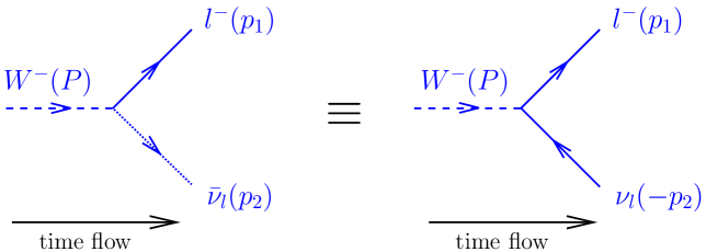
The leptonic decay can be of any type (electronic, muonic or tau) since all leptons can be considered to be massless. Indeed, in the Rest Frame (RF) each charged lepton have an energy of the order of , hence the charged leptons have a Lorentz factor of making out of them ultra-relativistic particles222In fact for the case of the , taking into account its mass eventually leads after computation to affect the width at the level of , but we consider this to be negligible in the context of our discussion.. The amplitude of probability of this process is
| (2.17) |
In this last equation, the weak force is embedded in the strength that couples particles sensible to the weak interaction and by the nature of this coupling represented by the co-variant bi-linear term of Vector–Axial () form. The coupling constant is usually expressed as a function of the Fermi constant that was formerly used when modeling weak interactions as contact interactions when occurring at energies scales much lower than . For historical reasons they are linked through the relation
| (2.18) |
The polarisation state of helicity is represented by the four-vector , is the spinor of and that of . We use here the convention which tends to consider that anti-fermions going forward in time can be treated on the algebraic level as fermions going backward in time. The spinors of backward traveling time fermions are noted for convenience. Let us note in the term the operator which, applied to a spinor , projects only its left-handed component
| (2.19) |
while the operator projects the right component of the latter
| (2.20) |
In other words, the presence of the term in the current couples only left-handed fermions and right-handed anti-fermions in electroweak interactions.
Usual “diracologic” calculus techniques allow to calculate , which corresponds to the Lorentz co-variant expression of the squared amplitude summed and averaged with respect to all possibles spins states for the and leptons. The differential decay rate writes in the RF
| (2.21) |
where , the Lorentz invariant phase space assuring energy-momentum conservation, can be reduced here to
| (2.22) |
where the energy and solid angle are those of the charged lepton. After the integration over the whole accessible phase space to the particles, the partial width of this process reads
| (2.23) | |||||
| (2.24) |
which is a Lorentz scalar. The result is the same when considering the case of the decay. The reader willing to have further details on the previous development or how to undergo such perturbative calculation, can go to classic references in particle physics/quantum field theory such as Refs. [59, 45].
This first order expression for the partial width allows to calculate the total width of the or the . The can decay into leptons or into a pair of quark–anti-quark that in turn decay to observable hadrons with a probability of one
| (2.25) |
For the leptonic decay, in the ultra-relativistic approximation assumed so far, the width is simply
| (2.26) | |||||
| (2.27) |
For the hadronic decay, the calculus is similar to the one for the leptons except that here : (1) CKM matrix element intervene and mix the quarks flavors and (2) in top of summing/averaging on the quarks spin states the sum and average on their color charge states need to be done as well. The can decay into all quarks flavors but the top which is forbidden by energy conservation since . The quarks possess masses such that they can be treated like the charged leptons as ultra-relativistic particles. Then studying gives for the partial width
| (2.28) |
where is the color number, the element of the CKM matrix governing the mixing angle between flavors and . Summing over all quarks flavors in Eq. (2.28) gives
| (2.29) |
where the sum on of the squared CKM elements translates the unitary of the CKM matrix and where is restricted to and flavors since the decay to the top is forbidden. Then in this context
| (2.30) |
Adding both leptonic and hadronic parts gives eventually in the Born level approximation
| (2.31) |
where has been replaced by its explicit form. Adding QCD corrections in quarks decays transforms the latter expression to
| (2.32) |
where is evaluated at the energy scale imposed by the mass. Following those developments it is assumed in the rest of this thesis that .
(b) Polarised bosons
Considering the leptonic decay of a real boson with a specific polarisation state proves to be very helpful to understand the angular decay behaviour of the quarks or leptons. The polarisation states of the two transverses () and the one longitudinal mode of a of momentum can be expressed in the laboratory frame like
| (2.41) |
Transverse polarisation states.
The example of the leptonic decay of a is again considered, for a polarisation state of . Substituting the expression of in Eq. (2.17) gives the probability amplitude for . This amplitude squared and averaged on the leptons spins, gives the term from which the differential decay width, in the RF is
| (2.42) |
Developing that expression gives, in the end, an angular dependency of
| (2.43) |
where the angle is defined like
| (2.44) |
The angular dependency in Eq. (2.43) is an important key for understanding the leptons kinematics in the decay. It can actually be understood without going to refined calculations but using only the helicity conservation rules in the high energy limit imposed on the leptons by the mass of the . As it was seen previously the electroweak interactions couples only left-handed fermions and right-handed anti-fermions. In the high energy limit chirality and helicity becomes the same, which means that the helicity is a conserved quantum number and only negative (positive) helicity fermions (anti-fermions) are involved. This explain why sometime in the literature, as a shortcut, but only in the high energy limit, negative helicities states are referred to as “left” and positive states as “right”.
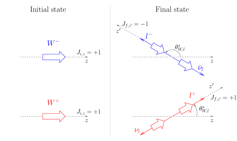
Now the previous example is treated from the helicity conservation point of view. The decay is depicted in the RF in the upper part of Fig. 2.2. The convention for the axis is the following. In the initial state the direction is parallel to the direction of the momentum of the in the laboratory frame while the direction points to the direction of the decaying charged lepton in the final state. In that context, the decay proceeds from an initial state with to a final leptonic state with and in both cases the system holds a total spin of , thus the amplitudes are proportional to the rotation matrices, it reads
| (2.45) |
which expressions for commonly used spins are tabulated in many places, e.g. Ref. [1], then
| (2.46) | |||||
| (2.47) |
Thus the most privileged configuration is the one where the initial and final spin projection and are aligned, while on the other hand the configuration where the would be emitted such that would be totally forbidden by helicity conservation.
The case of the decay of the can be deduced using the same kind of argument except this time the charged lepton is “right” and the neutrino is “left” as shown in the lower part of Fig. 2.2, the angular dependency is then
| (2.48) | |||||
| (2.49) |
Longitudinal polarisations state.
For the decay of a possessing a longitudinal polarisation state a detailed calculus can be carried out using the expression of with and in the RF. Instead of doing so the angular dependency, that really matters, can be unraveled using again rotations matrices
| (2.50) | |||||
| (2.51) |
In this equation in the case of a decay and for the one of a . Here there are no differences in the angular decay between the positive and negative channels.
Sum up for the decay of polarised W.
The previous derivations can be generalised to include in the formulae both the boson charge and helicity
| (2.52) | |||||
| (2.53) |
The sign in front of can be deduced easily each time by deducing which direction is privileged for the charged lepton from helicity conservation arguments point of view.
2.4.2 W in Drell–Yan-like processes at the LHC
The Drell–Yan [60] processes were originally defined, in hadron–hadron collisions within the parton model, before identifying partons with quarks and later on, with gluons. In these processes, a pair of partons, the hypothesised building blocks of nucleons, collide and annihilate giving in the final state a high invariant mass lepton pair . Within QCD, this partonic reaction proved to be achieved at first order, by the quark–anti-quark annihilation via . The main features of the formalism describing Drell–Yan survived to the rise of the QCD up to a few refinements. Still, for historical reasons even though the whole present discussion takes place within QCD the term parton is still used and refers to quarks or gluons.
By extension the production of high invariant mass pair through the production of an intermediate boson is referred to as “Drell–Yan like processes”, or –for convenience– Drell–Yan. Below reminders of the treatment of boson production in Drell–Yan is given. Let us remark that the formalism described is applicable to the original Drell–Yan and to a wide variety of over hard scattering processes including jet and heavy flavour production. Further general details on this topic can be found in Refs. [61, 46, 62].
(a) Overview
The production of a in Drell–Yan can be written
| (2.54) |
The associated Feynman like representation of this process is shown in Fig. 2.3, where and are hadrons of four-momenta and accelerated by the collider bringing a total energy in the center of mass. The collision produces a pair of leptons of four-momenta and . The other particles produced in this collision noted are not considered at all. The derivations that follow are applicable to the decay in the channel, nonetheless the analysis being restricted to the electronic and muonic decays, throughout the whole document unless stated otherwise.
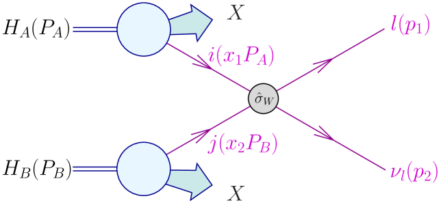
The hadronic cross section for a given point of the quarks and leptons phase space, , and for a particular collision of partons and can be expressed using the factorisation “theorem” like
| (2.55) |
that is as the product of the partonic cross section and the parton distributions functions (PDFs) and .
The PDFs are the density probabilities and for two partons and , to carry before their hard scatter fractions and () of the four-momenta of the hadrons they respectively income from. Purely theoretical derivation of PDFs are not computable as their description falls in the non perturbative regime of QCD where is too large, therefore they are extracted from global fits to data from processes such deep inelastic scattering, Drell–Yan and jet production at the available energy range fixed by colliders. The implementation of QED and QCD radiative corrections from quarks in the initial state are universal, i.e. independent from the process. These corrections contain mass singularities that can be factorised and absorbed in a redefinition (renormalisation) of the PDFs. The singularities are removed in the observable cross section while the PDFs becomes dependent of a factorisation scale controlled by the DGLAP evolution equations [30, 31, 32]. This scale is to be identified –for example– to a typical scale of the process, like the transverse momentum or in the present case by the mass of the resonance .
The partonic cross section corresponds to the probability that the partons and , of four-momenta and , collide and create a resonance of mass which in turn decays into leptons and respectively of four-momenta and . The hard scattering occurs at such energies that partons can be seen as free, i.e. is small. This allows to calculate the cross section using perturbation theory. Up to a given energy scale higher order Feynman diagrams are not directly computed but accounted by factorising their effect in the value of the constant . This renormalisation scale is the one of the virtual resonance, which means here . The total partonic cross section is then developed in power of
| (2.56) |
In this equation the first term of this series is the leading-order (LO), usually called the Born level, the second the next-to-leading order (NLO) correction of order and so on the third term adds up next-to-next-to-leading order (NNLO) corrections of order . The last term contains all corrections above . In practice only the first corrections are brought to a calculus as the number of Feynman diagrams increase rapidly when going to higher order corrections. Let us remark that a correction term of order is to be implicitly apprehended as where
The total hadronic cross section is then deduced by embracing all available corrections to the partonic cross section and by successively integrating Eq. (2.55) over the accessible phase space to the leptons and partons. This means in the latter case integrating over all possibles and , but also by summing over all possible partonic collisions, which gives eventually
| (2.57) |
From the experimentalist pragmatic point of view the matter of importance is to understand the kinematics of the leptons and how the properties can be extracted from them. Hence, in what follows, basics on the partonic cross section and on the PDFs are reminded with emphasis on the kinematics aspects rather than the dynamical issues. After that, an overview of the relevant kinematics in production is given.
(b) Partonic level
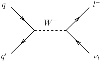
The production of a at the Born level is made through quark–anti-quark annihilation, which is illustrated here for the case of a and noted
| (2.58) |
where the four-momenta of the particles have been put into brackets. This process, described by one Feynman diagram (Fig. 2.4), has an amplitude of probability expressed as
| (2.59) |
The pending expression for the process is obtained by doing the substitution and in this last equation. Let us note that in the case where , that is for a low energy in the collision, the propagator of order makes us rediscover the historical coupling constant from the Fermi model.
At Born level all partons have a purely longitudinal motion, which means that in the present convention, the quark and anti-quark momenta are expressed in the Cartesian coordinate basis like
| (2.68) |
The total partonic cross section deduced from Eq. 2.59 reads
| (2.69) |
where and are the spins of the quark and of the anti-quark. The previous formula is correct as well in the case of a production. The variable belongs to a set of three others invariant Lorentz scalars, known as the Mandelstam variables, and is defined by
| (2.70) | |||||
| (2.71) |
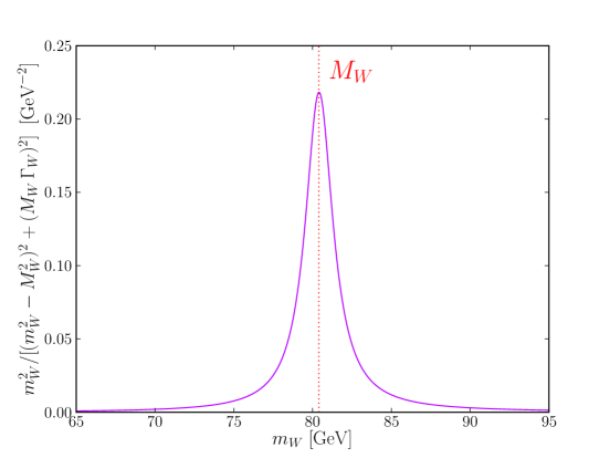
where the last line makes the link with the invariant mass of the off-shell . The fraction in Eq. (2.69) depending of reveals the Breit-Wigner resonant behaviour of the , that is a peaked distribution centered on and whose width is controlled by . It means a can be produced at any mass, as high or low as possible, but the probability this happens gets smaller and smaller as is far from the central value of the peak like as shown on Fig. 2.5.
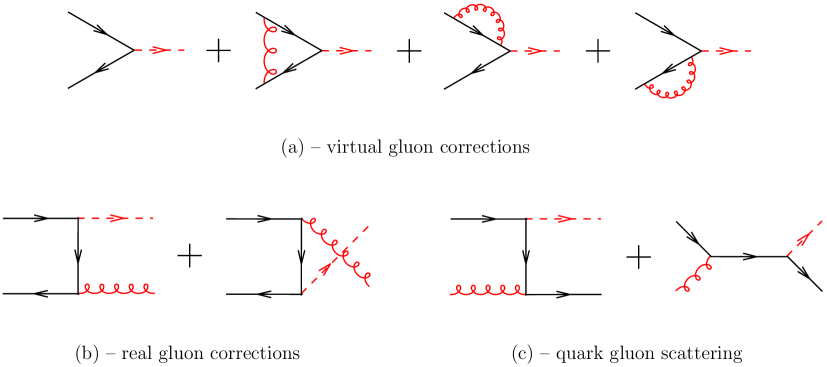
The NLO corrections of comes from the three following contributions in which represents a virtual photon : (a) virtual gluon corrections to the LO , (b) real gluon corrections and (c) quark/anti-quark gluon scattering , or . The Feynman diagrams associated to these corrections are displayed in Fig. 2.6 (a), (b) and in (c) for the case of quark gluon scattering only.
In top of QCD corrections are electroweak radiative corrections briefly mentioned below. The EW radiative corrections to the in Drell–Yan can be divided in a gauge invariant way into three parts : the initial state radiation (ISR), the initial-final state interferences (non factorisable corrections) and the final state radiation (FSR). The leading ISR (mass singular) QED corrections can be absorbed as stated previously into the PDFs. The non factorisable corrections are negligible in resonant boson production [63]. On the contrary, the FSR corrections affect considerably various observables among which is the transverse momentum of the charged lepton whose shape is primordial for the extraction of the . For example in Ref. [64], the final state photonic correction was approximated and lead to a shift in the value of of for the Tevatron collisions at that time. The development of these electroweak NLO corrections is beyond the scope of our discussion, the reader interested to have more details on this particular topic can look at Refs. [63, 65].
Coming back to the LO, before the phase space integration the differential partonic cross section can be written as a function of ,
| (2.72) |
the angular dependency can be traced back from the derivations made in Eq. (2.52), and where in the present context the polarisation of the is ruled by the following inequality between the fractions of momenta and the partons bears before the collision
| (2.73) | |||||
| (2.74) |
Note that at the LO there are no production of of longitudinal polarisation state due to the absence of a transverse momentum of the and in the massless quark approximation. Nonetheless, from the algebraic point of view, rather than the , the quarks and leptons are the objects we manipulate, hence in the continuity of the present calculus Eq. (2.72) writes in function of –the angle between the charged lepton and the quark momenta– like
| (2.75) |
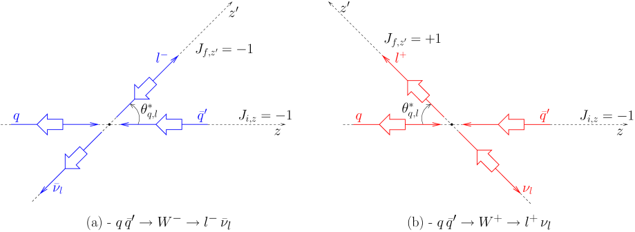
The angular dependency can be found out quickly using the rotations matrices techniques. Figure 2.7 actually gives the hint for the privileged angular decay configuration constrained by helicity conservation, for both and cases. For example in the case of , using rotation matrices techniques with the help Fig. 2.7.(a) gives
| (2.76) | |||||
| (2.77) |

Based on Eq. (2.75) the partonic cross section can be expressed as a function of the transverse momentum of the charged lepton in the RF . This function will be be useful later to understand the behaviour of the charged lepton in the laboratory frame. The change of variable is done by summing the two angular configurations giving the same as shown on Fig. 2.8. The analytical derivation writes
| (2.78) |
which gives finally
| (2.79) |
From the jacobian arise a term whose denominator shows a singularity when . This singularity is visible in Fig. 2.9 that represents the distribution and for that reason it is called the jacobian peak.
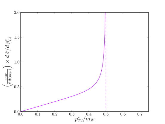
This means this peak will eventually be visible at the hadronic level but will be smoothed when integrating over all possible masses for the . Still, because the distribution is weighted by only the contributions for which the invariant mass is such that will be preponderant (cf. Fig. 2.5). Therefore a peak is to be expected around its smoothness being a direct consequence of the width .
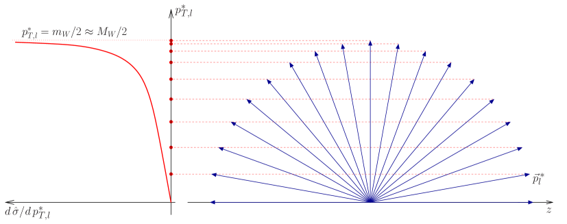
The jacobian peak in the distribution can be understood from a more intuitive geometric point of view that consists to project the momenta of the charged lepton on the transverse plane like shown in Fig. 2.10 where an isotropic decay of the charged lepton has been adopted for representation practicability. As as can be seen the rise of the is a direct consequence of the function entering the projection .
(c) Behaviour of the parton distribution functions
Here the PDFs behaviour in function of are reminded because of their strong influence on the kinematics of the and in consequence on the leptons. The quantity represents the probability to have a parton of type in a proton having a fraction of the four-momentum of the latter comprised between and . Figure 2.11 represents the PDFs extracted from the set CTEQ6.1M [66] used in this analysis.
Two type of partons can be distinguished in a proton, the valence (v) quarks and the sea (s) quarks. The valence quarks –bound by the strong interaction– are the elementary particles conferring to the proton its properties. The sea quarks arise as a consequence of the short-time fluctuation of the wave function of the proton. As described in relativistic quantum physics particles can create and annihilate, which translates in the present case that valence quarks/gluons radiate gluons which in turn can split again in gluon or pairs of quark–anti-quark. A way to look at those distributions is to consider that a probing particle impinging on the proton can resolve in the transverse direction its smaller building blocks as better as it possess a high energy. Indeed, using optics vocabulary, to a probe of momentum we can associate an intrinsic wave-length which is most likely to diffract with pattern of the same wave-length. Bearing this fictitious probe in mind the behaviour of each flavours are recaptured.
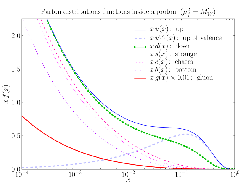
The up and down quarks are predominant compared to any other flavors which means that as we would expect a probe will most likely hit a or a in proton. Near the bumps reflect the high probability to hit a valence or quarks. In Fig. 2.11 the valence contribution for the case of the up quark is shown. Thus, the rise of the probability at low is due to the sea contributions starting from 0 at and increases as . The behaviour at small- is the consequence that probe starts to resolve more and more of de-localised sea quarks. The and behaviour can be directly deduced from the removal of the valence bump present for the and flavors. Let us stress than even though the masses of the and quarks are very close for we observe that .
The patterns in the strange, charm and bottom quarks can be understood from the previous explanations for the up and down quarks of the sea. For a given the probability to observe a given flavour decreases as the quark mass increase. Indeed, it is harder to create virtual pairs of heavy quarks compared to lighter quarks given the same amount of energy explaining why . Concerning the top flavour the energies scales we are working with are far too small to resolve any top quarks hence, . The distributions of the , and are exactly the same in a first approximation. For example, only very recently the strange quark asymmetry has been implemented in some PDF set. Such corrections are not present in the CTEQ6.1M set that was used in this work, then later on .
Finally there is the gluon contribution that needed to be divided to a factor of to be scaled to the frame.
(d) Hadronic level at the improved leading order
Higher order corrections are necessary to get rid in the cross section as much as possible of the dependency from the unphysical renormalisation and factorisation scales due to the perturbation expansion truncation. Nonetheless, the comprehension of the main features of the and leptons kinematics can be done studying just an improved leading-order description of the phenomenon, and when necessary, use higher order corrections to pin-point a particular effect in a given phase-space domain.
This improved LO, considered in the rest of this Chapter, is defined by taking the LO expressions of the partonic cross section convoluted with the remormalised PDFs and by taking part of the radiation of the partons in the initial state. Due to momentum conservation, the radiation of gluons and photons off partons provide a realistic picture in which quarks produce a with a non zero transverse motion. Note that by “part of the radiation” we mean that emission of real gluons and photons are taken into account but without embracing all other virtual loop corrections belonging to the same order in or . In this scheme, Fig. 2.12 represents an example of such initial state radiation for a particular event.
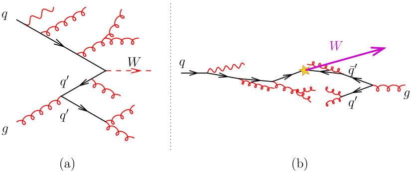
Before going any further common variables and conventions are reminded. Usually, switching to a second set of variables equivalent to proves to be useful. This change of variables is defined by
| (2.80) | |||||
| (2.81) |
At leading order, using the expressions of the quark and anti-quark momenta from Eqs. (2.68) gives for the rapidity the expression
| (2.82) |
which for and when expressed in function of and give the following expressions
| (2.83) | |||||
| (2.84) |
To get rough estimations, in top of relying on LO expressions, the “narrow width approximation” is commonly used, it is defined assuming , the consequences for the mass and being then
| (2.85) | |||||
| (2.86) |
where for reminder in the case of collisions at the LHC. The numerical value in the last equality gives an idea of the percentage of the total energy needed to produce a . In this approximation the partonic cross section at LO can be expressed with a Dirac function. The Breit–Wigner term in Eq. (2.69) becomes333For reminder the Cauchy-Lorentz function tends to a Dirac distribution as reaches zero with positive values.
| (2.87) |
that is any dependency from vanishes, the partonic cross section is a constant which is non null only if the energy of the partons in the center of mass exactly equals .
The gist of the and leptons kinematics are illustrated below with the process , that is merging both positive and negative channels and looking at the and leptons kinematics. The Monte Carlo used to produce these preliminaries pedagogical histograms is WINHAC which will be described with more details in Chapter 4. All Monte Carlo predictions in this document are, unless stated otherwise, produced using WINHAC. The derivations presented below will serves as a base to understand later on with more refinement the production of for each electrical charge channel separately.
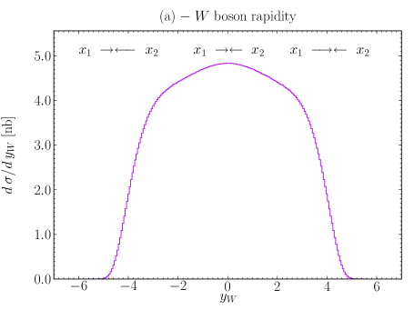
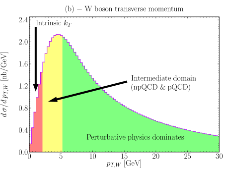
Rapidity of the W boson.
In the improved LO picture the rapidity approximately equals the LO expression Eq. (2.82), that is . This form translates an unbalance between the fractions and , and explains why the rapidity is strongly correlated to the PDFs. To the leading order approximation we add the one of the narrow width, in that context the and fractions entering the PDFs now reads
| (2.88) |
The pattern of the rapidity distribution can be devised only from the previous expression, the weight from the partonic cross section being just a multiplicative factor.
The range for the rapidity can be deduced using the constraints on and
| (2.89) |
which means a higher energy in the collision provides more kinematic energy to the while its mass reduces this kinematic energy. Replacing in Eq. (2.89) and by their values one find that at the LHC the rapidity range is approximately as displayed in Fig. 2.13.
The rapidity distribution tends to zero when because one of the fraction is necessarily tending to and as seen previously . Considering, in a first approximation, that fractions are of the order of one find that in average while for the Tevatron energies . This shows how the energy in the LHC collisions will make small- contributions predominant with respect to the one of the Tevatron.
In the region , the form of the rapidity seen in Eq. (2.82) indicates that , which happens for sea quarks most of the time. Indeed, substituting in Eqs. (2.83–2.84) and gives . For these values of the probability of having a valence quark is small, most contributions comes from sea quarks.
On the other hand, in the forward rapidity region, there must be an important unbalance between and . In an extreme case scenario, this condition is fulfilled when a quark bears an important fraction while the other one possesses a very small fraction , which is most probably occurring when a valence quark and a low energy sea quark collide. This can be shown using rough values, substituting again in Eqs. (2.83–2.84) and gives, and . The fall of the rapidity, occurring at , is then a consequence of the fall of the valence quarks PDFs densities as .
Let us remark that the impossibility to measure the neutrino longitudinal component implies that while trying to resolve it using the other measurable kinematics one ends up with an equation of second degree in with two solutions leading in turn to two ambiguous solutions for . Nonetheless, even if the problem is not solvable on an event-per-event basis, some solution based on the whole data event allows to partly overpass the problem in the narrow-width approximation [67].
Transverse momentum of W boson.
The distribution of (Fig. 2.13.(b)) in this improved LO picture is the consequence of three main effects. First is the perturbative emission of real gluons and quark/anti-quark gluon scattering (Fig. 2.6.(b,c)) which dominates at high . As decreases the spectrum is governed by the re-summation of leading-logs, then finally below the intrinsic transverse momentum of partons inside the proton dominates.
Since the intrinsic of partons modeling enters our analysis more details are given below. This intrinsic can be initially apprehended as the consequence of the Heisenberg uncertainty principle applied to the confinement of the partons in a finite volume of the order of a Fermi. Still, a quick calculus shows this effect cannot totally account for the observed data and this initial is nowadays depending on the energy involved in the collider. Assuming a simple factorisation of this effect from the longitudinal motion ruled by the PDFs the expression of the latter necessary to the cross section calculus can be accounted doing the following substitution
| (2.90) |
where is the density of probability for a parton to have a transverse momentum of . Modeled with a Gaussian distribution it can reads :
| (2.91) |
where the average value of noted is . This values needs to be estimated for a particular collider to match to the data. In the case of the Tevatron energies it is estimated to be of and should be higher at the LHC.
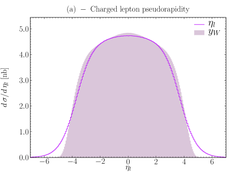
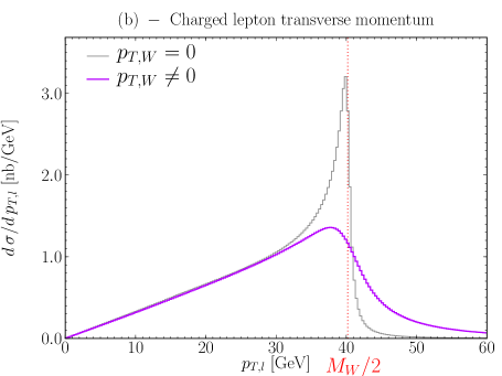
Pseudo-rapidity of the charged lepton.
The pseudo-rapidity of the charged lepton is obtained by adding to its intrinsic rapidity in the RF the rapidity of the , it reads at LO
| (2.92) |
The rapidity of the , as shown previously, is related to the energy in the collision and the mass of the while the intrinsic rapidity is a consequence of the angular decay governed by the coupling. Indeed, still at LO, takes the form
| (2.93) |
The estimation of the contribution of the intrinsic rapidity of the lepton to the total pseudo-rapidity can be evaluated roughly. We make the assumption that in average there is as much charged leptons spreading the fundamental distribution that narrowing it, which can be formalised stating there is as much than . Substituting these averaged values of in Eq. (2.93) gives , i.e. . Then, the main pattern of the distribution is mostly inherited from the one present in the distribution. This explains why distribution covers sensibly the same range than as can be seen in Fig. 2.14.(c). Because the rapidity cannot be measured the distribution is used as a substitute and proves particularly useful in the PDFs study. More details on that topic in the context of the ATLAS experiment can be found in Ref. [68].
To be completely honest here, and tease the reader’s curiosity, the assumption that spreading and narrowing behaviour of the distribution occurs in the same proportions is more or less verified at the Tevatron but it will not be the case at the LHC. In the latter case the tends to narrow the inner spectrum while the spreads the latter. Then, the previous calculus is justified since both charge being merged the narrowing and spreading compensate each other and also because .
Transverse momentum of the charged lepton.
The distribution for the transverse momentum of the charged lepton at the hadronic level is directly linked to the one at the partonic level. At leading order, which implies . Then a jacobian peak around is visible, its smearing coming from contributions in which . Contributions displaying a value too far from the central value are, as it was shown in Eq.(2.79) highly improbable. Then, the distribution which is observable in a detector presents a jacobian peak which position allows to deduce the value of .
Things gets more complicated when going to a more realistic scenario where the possesses a transverse motion. To understand that the relative angle between and in the plane noted is considered. The sign of give rise to ambivalent behaviour for . In the first case, where , is such that the total Lorentz boost based from increase the value of . In such events then are shifted to higher values, to the right of the Jacobian peak. On the contrary, in -cases are decreased, that is shifted to the left of the Jacobian peak.
Figure 2.14.(b) shows how much the transverse momentum of the smears the sharpness of the Jacobian peak. That means that the extraction, from the bare distribution, of with a Monte Carlo imply a refined implementation of the .
Transverse momentum of the neutrino.
The transverse momentum distribution of the neutrino displays the very same features than the one of the charged lepton. Still from the experimental point of view, it is very different as can be deduced only from the missing transverse energy given by the entire response of the calorimetry of a detector. For that reason is preferentially noted or . The calibration of the missing transverse energy needs at least a few years, and even after that it cannot compete with the study of the charged lepton, indeed as can be seen in Table 2.3 the CDF II results [51] shows large systematic errors on when using the distribution.
Transverse mass of the lepton pair.
The transverse mass was suggested in Refs. [69, 70] to provide an alternative to measure the mass and width of the boson. It consists of calculating the invariant mass the lepton pair would have if and would be null. For that reason it is called the transverse mass444This definition of the transverse mass should not be confused with the one introduced sometimes in relativistic kinematics and defined as , like for example in the Kinematic review in Ref. [1]. is defined like
| (2.94) | |||||
| (2.95) |
Now since the transverse momenta of both leptons enter as a product the influence of upon is counterbalanced by the opposite effect upon . At LO in the RF both leptons transverse momenta are equal, a purely longitudinal boost does not affect these values, hence and which gives for the transverse mass the , explaining why in this case the jacobian peak is located at .
Figure 2.15 represents the and distributions for three different steps in the simulation of in Drell–Yan inside ATLAS [71]. Note that in each step trigger and acceptance cuts were made according to the ATLAS requirements, in particular and cuts can be clearly distinguished looking at the low region of the histograms, for further details see Ref. [71]. The first case considered is the true level, that is the prediction from the Monte Carlo at pure leading order where . Both and jacobian peaks are sharp. When adding up QCD corrections in the initial state the jacobian peak of is very smeared by , while still displays a sharp jacobian peak. The last step consists to pass the latter event generations to a simulation of the ATLAS detector. The good resolution for the charged lepton does not change a lot, while the bad resolution for smears a lot the jacobian peak of .
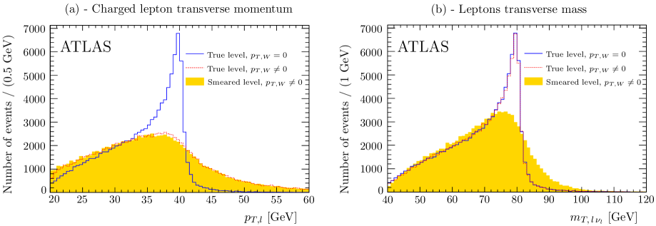
| Distribution | [] | ||
|---|---|---|---|
2.5 An invitation to the rest of the document
Up to now, the motivation and the general context for a measurement of the charge asymmetry within the Standard Model paradigm have been described. Now the outline of the rest of the document is presented through a short description of each Chapter aims and content.
Chapter 3 presents the experimental context in which this measurement can be achieved, that is at the LHC and more precisely with the ATLAS detector. Especially, the emphasis is made on the ATLAS tracker since the analysis was restricted using this sub-detector capabilities. Some highlights are made on the deformations of the tracker that should increase the systematic errors on .
Chapter 4 presents the tools that were used or implemented to carry out our analysis to evaluate the ATLAS potential to measure . It almost exclusively treats about the Monte Carlo event generator WINHAC. The physics inside it is described along with the tools implemented downstream for the stand-alone analysis that was made. The Chapter describes as well the work done to include this Monte Carlo event generator inside the ATLAS software environment.
Chapter 5 presents the detailed work that was done to understand the kinematics of the and at the LHC made necessary for the prospect of the measurement of but as well as for our other ongoing effort made on properties extraction such as [72, 73] or [74]. Actually we consider this Chapter to be of interest for every physicist working on the production in Drell–Yan at the LHC, for ATLAS, CMS and even LHC detectors.
Chapter 6 presents dedicated strategies to measure and their qualitative evaluation. After a short introduction of the general experimental context (trigger, acceptance, background, etc.) the analysis strategies devised to measure the boson mass charge asymmetry. The strategies were specifically designed for this measurement to get rid as much as possible of the dependency from both Monte Carlo and apparatus imperfections to decrease the impact of systematic errors on .
A Conclusion closes the document by summing up the results obtained with the proposed methods and, by taking a step backward, localise the importance of the present work amid the ongoing effort on precision measurements of the boson properties at the LHC.
Chapter 3 The ATLAS experiment
Atlas : “Where is he ? Where is your titan ?! I will show him sorrow! I will show him pain ! I will show him Atlas ! I am the champion this city, this land, this orb needs.”
Superman #677 - In The SHADOW Of ATLAS (August 2008)
The Large Hadron Collider (LHC) [75, 76, 77, 78, 79] will be the largest circular accelerator of hadrons ever build providing unprecedented energy and luminosity. It is buried underground within the CERN [80] facility near Geneva. This accelerator was designed to fulfill the increasing needs to probe ever smaller lengths scales to unravel the nature of the interactions of elementary particles. For that purpose the LHC accelerates in its ring counter rotating bunches of hadrons at ultra relativistic speed and collide them in four distinct points. The particles produced during these collisions are studied using one or several detectors built in the vicinity of each of the four interaction points. Among them is ATLAS [81, 82] a general purpose detector.
In this chapter, two of the most fundamentals collider parameters from the physicist point of view, i.e. the energy in the center of mass and the luminosity, are reminded in the LHC context. Then, the ATLAS detector is presented by reviewing the geometry and technology implemented within each of its sub-detectors : the tracker, the calorimeters and the muon spectrometer. Especially the tracker, which performances are used in this work, is described with more details. Some emphasis are made on the aspects relevant to the measurement of through the observation of the process where for reminder stands for .
3.1 The Large Hadron Collider
3.1.1 The collider
The need to produce physics resonances of ever higher masses at noticeable rates within colliders requires higher energy in the center of mass of the collision as well as higher luminosity . The importance of synchrotron radiation in collisions is such that it proved to be prohibitive above LEP [83] energies to use circular collider. Then, the idea of studying non collisions using the LEP tunnel began to be studied in 1984 [84] and at the time the LEP collider shutdown in 2000, the project of colliding hadrons was decided [75]. So far hadron–hadron colliders were designed for collisions like at the SPS or the Tevatron colliders. Above the cross sections for and collisions are comparable but for the latter case the luminosity would have been inferior to a factor at the LHC due to the difficulty to produce anti-protons. On the other hand collisions of particles holding the same charge impose a priori to have two independent rings having magnets of opposite polarity with separate cryostat which would have turned out to be more expensive. For the LHC a special two-in-one dipole magnet was conceived in the aim to be more economic and compact. Thus, collisions being more easily achievable and less costly it was the chosen option. The LHC will as well make collisions of heavy positively charged ions.
From the physics point of view the most striking difference between hadron–hadron and collisions is that in the primer case the colliding particles are composite and gives for each inelastic process of interest to the physicists an important number of other particles. Hence, the LHC is primarily designed for discoveries rather than for precision measurements, still, its high center of mass energy and luminosity combined to the detectors performances should allow precision measurements. Another consequence of the hadrons composition is that partons participating in an inelastic scattering borrow only part of the whole disposable energy . For the case of production in Drell–Yan we have seen in Eq. (2.86) that in average of is used.
Fig. 3.1 shows the different parts entering each superconducting magnet dipole that were assembled along the 27 km circumference of the LHC ring. Each proton beams are moving in opposite directions inside each of the two main dipole aperture beam-pipe. The dipole generates a magnetic field of to maintain the protons beams along the ring circumference, other magnets are present to focus and correct any deviations of the beams.
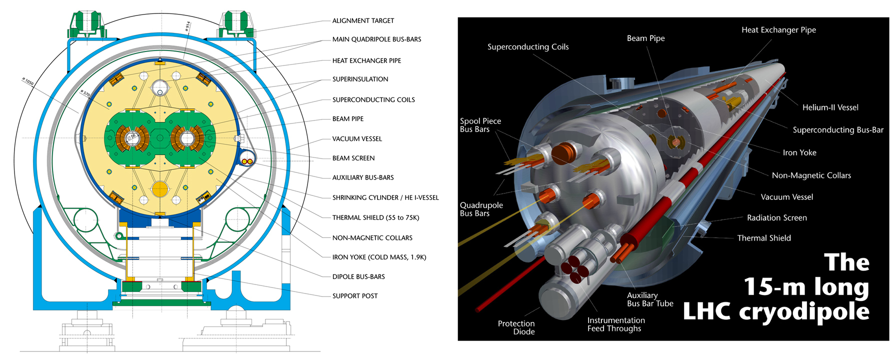

The different steps of the protons acceleration and injection inside the LHC ring are shown in Fig. 3.2. The proton beams, split in bunches of oblate volume, are successively accelerated by the LINAC2, the BOOSTER, the PS and the SPS accelerators. The SPS injects proton bunches of in the LHC superconducting magnet, half moving in one direction and the over half in the opposite direction. Each proton in a bunch has an energy of providing a total energy in the center of mass of . The total cross section and its inelastic part are approximately equals to
| (3.1) | |||||
| (3.2) |
The volume of a proton bunch can be defined using Gaussian functions which full widths at half maximum are, with respect to the -axis along which protons move, of in the transverse direction and in the longitudinal direction. Each bunch, composed of an order of protons, are separated by a time lapse of ().
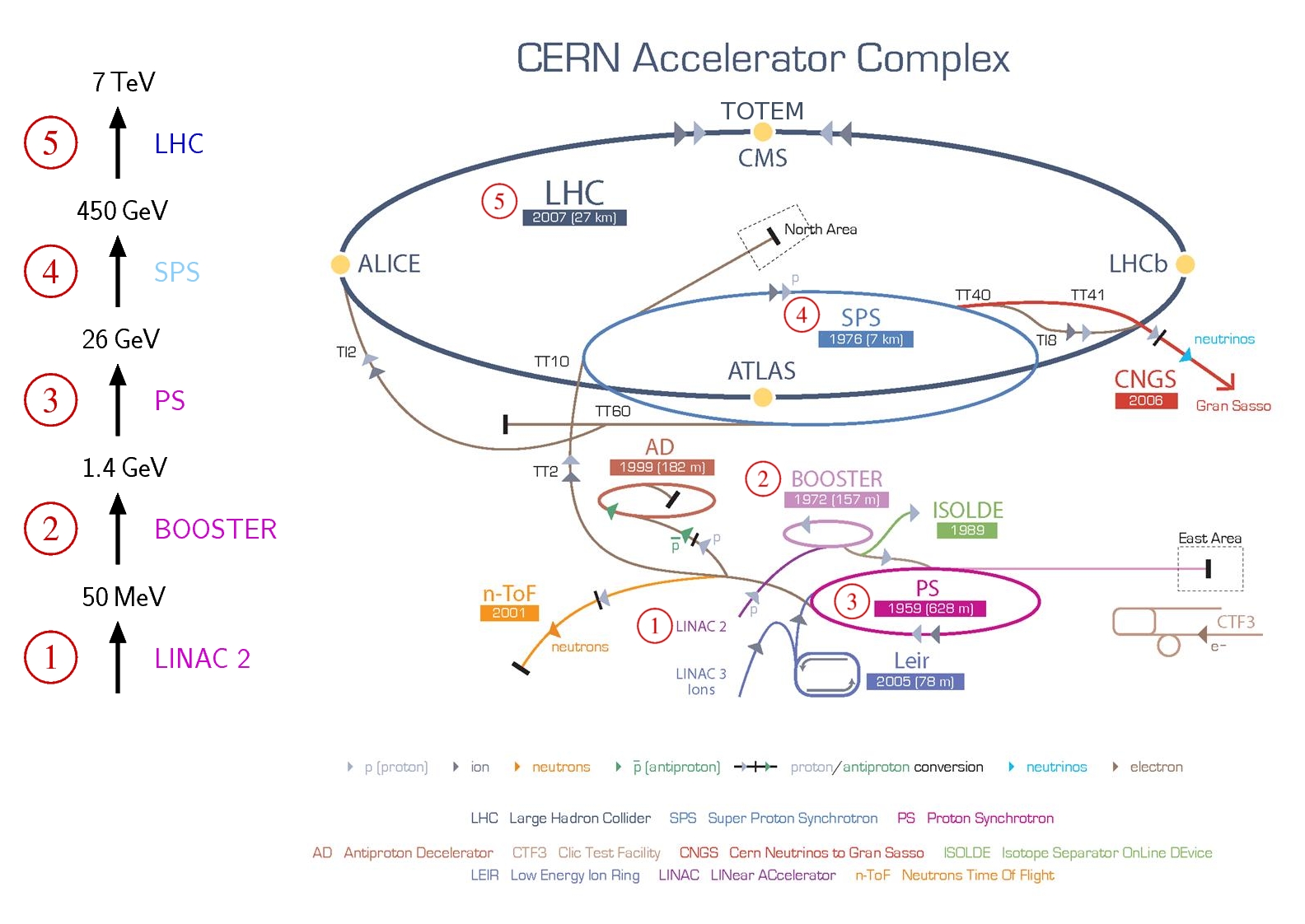
The luminosity is defined at the LHC like
| (3.3) |
where is the number of protons per bunch, the number of bunches, the revolution frequency around the ring, the relativistic Lorentz factor related to the proton velocity (), the normalised emittance and the beta function at the interaction point. The factor accounts for the reduction of interaction numbers due to the full crossing angle and other characteristics of the beam configuration, it reads :
| (3.4) |
The number of produced inclusive events for a process with an inclusive cross section over a time lapse is related to the integrated luminosity over via
| (3.5) |
The nominal luminosity of the LHC, expressed in several convenient unit should reach :
| (3.6) |
Based on Eqs (3.1,3.2), this gives a frequency of of produced events among which inelastic events occur at the rate of . This will eventually lead each event of interest to be accompanied by an average of inelastic events also referred to as the “pile-up”. For this reason the LHC will use during the first three years a lower luminosity for which the smaller pile-up ( events) will allow physicists to understand first the detectors before exploiting them at the design luminosity.
Most of the analysis in this work are considered for one year of LHC data taking at low luminosity, which, due to technical reasons, was assumed to be of the order of . Thus, one year of data taking in ATLAS at low luminosity implies an integrated low luminosity of
| (3.7) |
the choice for unit being cast on nb as the inclusive/cut cross sections are of this order.
The LHC ring is planed to accelerate and collide heavy ions as well. For the purpose of our measurement strategy the possibility of having run programs with light ions have been considered. In such a context the total energy of for the accelerated hadron is shared between the different nucleons building it. The energy of a nucleon belonging to an hadron of mass and charge is
| (3.8) |
Considering the collision of two hadrons and respectively of masses and the nucleon–nucleon () center of mass energy is where the energies and of each nucleon are computed using Eq. (3.8). Concerning the luminosity, it should be possible in the most optimistic case scenario to reach , corresponding to the standard integrated luminosity for collisions. In the present study, using these rules for the case of collisions that were occasionally considered, gives
| (3.9) | |||||
| (3.10) |
To sum up for and collisions, the nucleons energies and the integrated luminosity for one year at low luminosity are
| (3.11) | |||||
| (3.12) |
A number of produced events related to a process is computed using Eq. (3.5).
3.1.2 The LHC experiments
The detectors layout around the LHC ring is shown in Fig. 3.2. The actual approved experiments are : Alice, ATLAS, CMS, LHC, LHCf and TOTEM.
ATLAS (A Toroidal LHC ApparatuS) and CMS [85] (Compact Muon Solenoid) are two detectors made for general studies of the physics at the LHC, i.e. refine the Standard Model parameters, confirm/infirm the existence of the Higgs boson and study new physics signatures (hypothesised BSM models, new signatures). Both can measure the signatures of high objects such as , , , , jets, -jets, missing transverse energy , etc.
Alice [86] (A Large Ion Collider Experiment) has been created to study lead ions collisions to possibly materialise a state of matter known as quark–gluon plasma, which may have existed soon after the Big Bang.
LHC [87] (Large Hadron Collider beauty) is dedicated to the study of quarks decays in hadrons to understand the mechanism of violation that could explain the matter/anti-matter asymmetry in the Universe.
The LHCf [88] (Large Hadron Collider forward) experiment uses forward particles created in collisions as a source to simulate cosmic rays in laboratory conditions.
TOTEM [89] (TOTal Elastic and diffractive cross section Measurement) will measure the general properties of collisions such as the total cross section and the luminosity.
3.2 The ATLAS detector
3.2.1 Detector requirements
The ATLAS detector was designed in function of the expected physics signatures, the high energies involved in the hadrons collisions and the high luminosity context present at the LHC. This imposed high constraints over the detector performances, size and trigger system. Assuming an operation life of ten years or so the detecting devices and their associated electronics must stand high radiation due to the important particles fluxes. The other problem is that in average each inelastic scattering of interest that triggers the apparatus is accompanied by usually other non-interesting inelastic events. To decrease as much as possible this pile-up impact the detector needs, using a highly efficient trigger, to provide a precise and fast detector response. Also the detector needs a high granularity to lift as much as possible overlapping ambiguities between the processes of interest and the pile-up.
The size of the ATLAS detector is directly related to the energy scale of the produced particles which needs to be contained. For example, electrons of are absorbed by radiation length (), pions of by absorption length () and measuring momenta of muons of needs bending power of several . Another reason for the size of the ATLAS detector is the choice made for the magnetic field which, contrary to CMS, is separated in two pieces. The first one (solenoid) used by the inner tracking detector allows a good charged particle momentum resolution and reconstruction efficiency while the muons –not stopped by the calorimetry– have their momenta resolved by large magnets generating a toroidal over a large range of momenta.
Turning now to the events signatures, ATLAS needs to identify extremely rare events, some as low as representing of the total cross section. In the LHC context, lepton identification is challenging due to the high QCD background (e.g. the electrons jet ratio is ) and Higgs/BSM hypothesised signatures constrained strongly each sub-detectors performances.
These general requirements reminded, we give an overview of the ATLAS detector.
3.2.2 Overview of the ATLAS detector
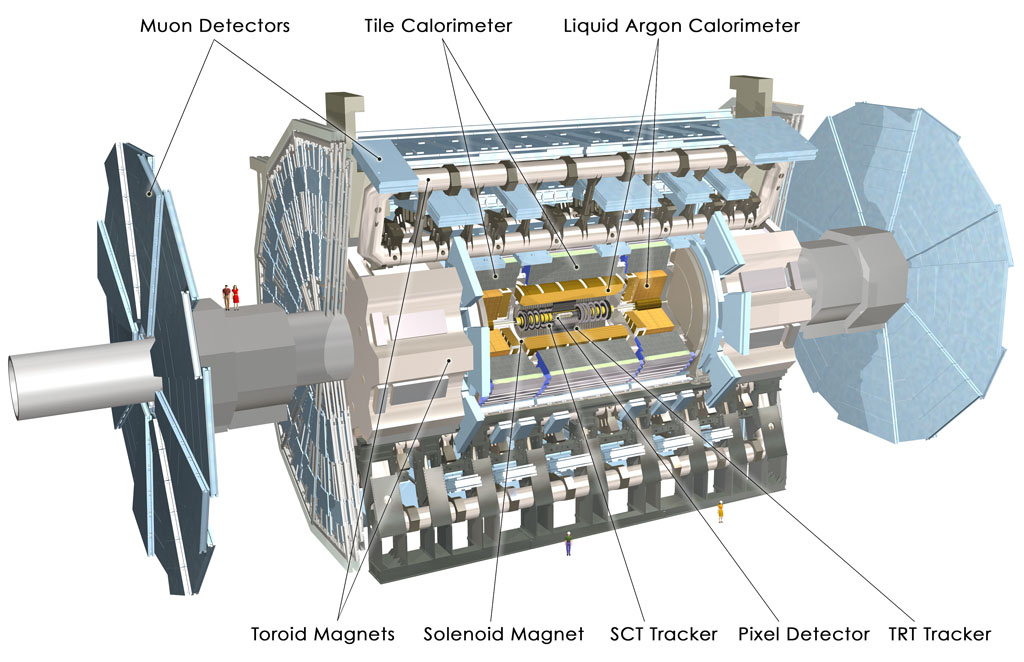
Detector.
The ATLAS detector is nominally forward-backward symmetric with respect to the interaction point. The sub-detectors layout follows basics rules common to all hadronic colliders. Starting from the beam-pipe one can find a tracking device, then electromagnetic and hadronic calorimeters and finally a detector for muons. The inner tracker and the muon spectrometer are immersed in magnetic fields generated respectively by a thin superconducting solenoid and three large superconducting toroidal magnets. This general setup can be seen in Fig. 3.3.
Each sub-detector is composed mainly of three pieces, a barrel for high particles and two end-caps located symmetrically from the interaction point to optimise the solid angle coverage. Usually, the transition regions between the barrels and the end-caps, also called the transition region, are used to pass the power cables and the readout cables of the devices.
First, the tracker, also referred to as the Inner Detector (ID), bathes in a magnetic field generated by a surrounding solenoidal magnet. It is made of semi-conductor silicon vertex detectors in the inner layers (pixel and semi-conductor tracker) and of straws trackers in its outer part. Charged particles, as they pass each layer, leave measurable hits that allow to reconstruct their trajectories and creation points (vertex) while their transverse momenta are deduced from their tracks deflection by the magnetic field.
After comes the sampling calorimeters made of alternate layers of absorbers and active detector medium. First is the electromagnetic (EM) calorimeter made of lead (absorber) and liquid argon (LAr) for the active medium. It measures with a high granularity and excellent performances in energy and position resolution the electrons and photons. The hadronic calorimeter measures the energy of hadrons and QCD jets. It is made in the barrel of steel plates (absorber) and scintillator-tiles (active detector medium), in the end-cap both tile and LAr calorimeters are used.
Around the hadronic calorimeter is the muon spectrometer bathing in the air-core toroid magnetic field. The high bending power of the magnetic field provides an excellent muon momentum resolution using three layers of high precision tracking chambers to detect the muon passage. Muons properties are measured using drift tubes and multiwire chambers. The spectrometer uses as well other chambers relying on cathode-plate and multi-wire chambers to trigger for high muons events. The muon detector defines the overall size of ATLAS which is of diameter and long. The total weight of the detector reaches tons.
Trigger.
The harvest of the data measured by those sub-detectors is achieved using a fast trigger. The trigger system selects events displaying interesting signatures among the plethora of events produced at the rate of at nominal luminosity. For the first time the collected statistic for large scale processes such as or production will be limited by the bandwidth and read out systems rather than by the produced events. The trigger is split into three Levels (L), L1, L2 and the event filter, the two last one being referred to as the high-level trigger. Each level refines the decision outgoing from the precedent level and, if necessary, apply additional selection criteria.
The L1 trigger treats subsets from each sub-detector information, it scans for high transverse momentum muons, electrons, photons, jets, leptons decaying into hadrons as well as large missing and total transverse energies. It also spots in each event to regions of interests defined as regions within the detector displaying interesting features. The decision to accept/reject an event is made within and decreases the rate of incoming events to . The L2 trigger reduces within the events rate to based on full data information within the regions of interested input by L1. The last stage of the event selection, made by the event filter, reduces the rate of events to . This step, lasting , is carried out offline using analysis procedure and supply an event of size Megabyte.
Already at this point we mention few trigger information relevant for both selection and analysis of properties from Drell–Yan production. More details will be given on these topics later on. Among few other requirements, the trigger should be activated for isolated electrons/muons with high threshold of the order of while the data from such events should be studied in the range .
Forward detectors.
Also worth mentioning are three smaller detectors in the forward region associated to ATLAS.
From the interaction point, at is
LUCID (LUminosity measurement using Čerenkov Integrating Detector),
at is ZDC (Zero-Degree Calorimeter)
and at is ALFA (Absolute Luminosity For ATLAS)
LUCID and ALFA roles are to determine the luminosity delivered to ATLAS and
ZDC to have a key role to determine the centrality of heavy ions collisions.
Figure 3.4 concludes this overview by recapturing the interactions of some particles with the different sub-detectors.
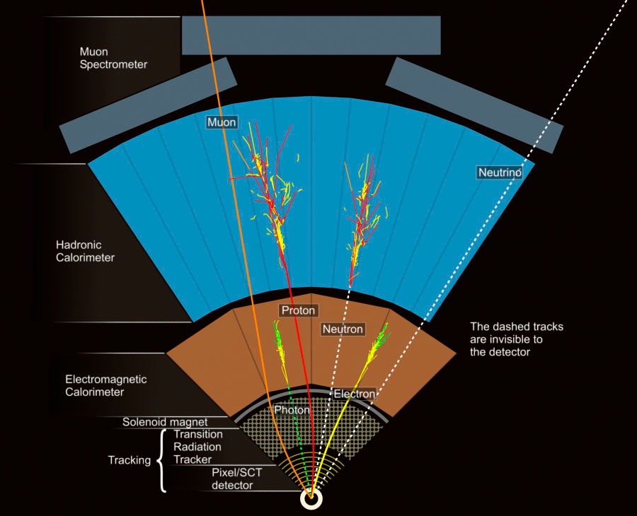
The rest of the Chapter presents the technology and geometry of each ATLAS sub-detectors. First the calorimeters and muon spectrometer are presented. In top of a general description, the link of their role on the measurement of in Drell–Yan is mentioned mostly from the trigger point of view since the tracker, so far, does not have any trigger on its own. Hence the electromagnetic calorimeter and muon spectrometer trigger efficiencies for events displaying respectively isolated high electrons and muons are cited. These kind of studies associates as well due to the final state neutrino. However, since in the present analysis the latter is not taken into account, the trigger is not considered to be relevant although its influence on the results was controlled. More details will be given in Chapter 6. In the second and final part, a detailed description of the inner detector is given. In what follows, dimensions of devices are given by their radial(longitudinal) extensions () and their absolute pseudo-rapidity acceptance .
3.2.3 Calorimetry
Both electromagnetic calorimeter (EMC) and hadronic calorimeter (HC) geometry, technology and performances are reviewed. Their set up can be seen in Figs. 3.5 and 3.8.
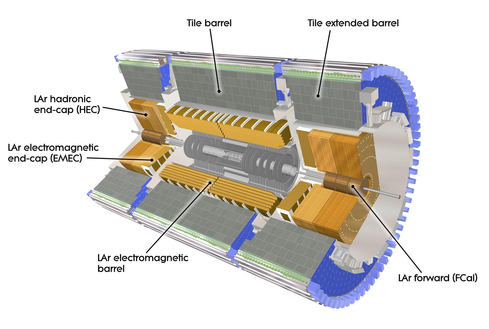
(a) Electromagnetic calorimeter
Technology.
The EMC [90, 91] is made of accordion shaped layers of lead plates-kapton electrodes bathing in liquid argon as depicted in Fig. 3.6. The accordion geometry, symmetric in , presents a full and crack-free azimuthal coverage. The readout of the high voltage electrodes are maintained at equal distance from two lead sheets using honeycomb spacers. A high energy electron or photon as it passes through an absorber looses energy respectively via bremsstrahlung or pair production . These produced particles in their turn interact with the other absorbers creating a shower of particles. Particles from this shower excite liquid argon from which ionised electrons –as they drift to the electrode– allow to find eventually the shape and the total energy yielded by the incoming electron/photon.
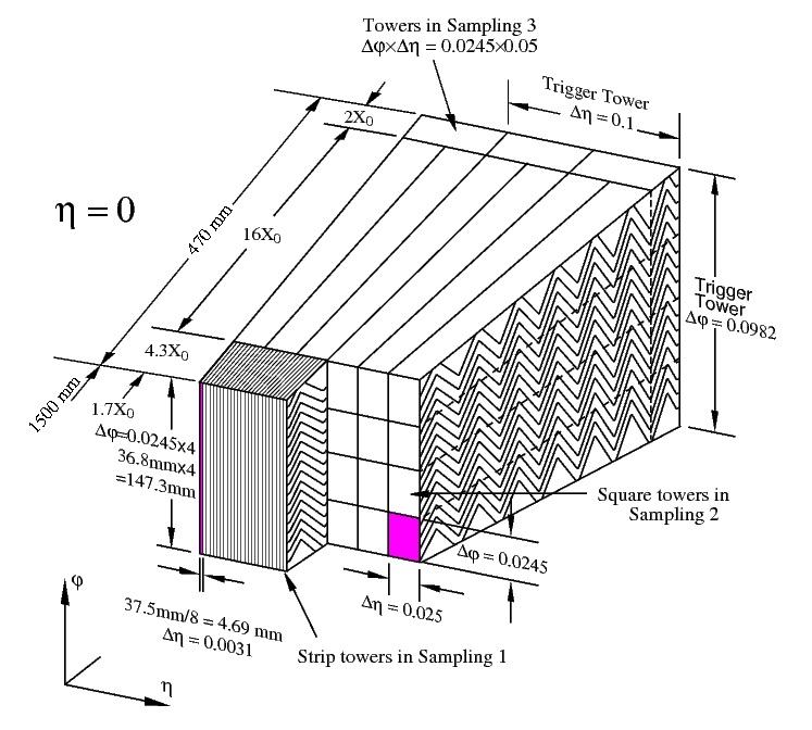
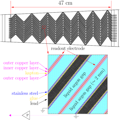

Geometry.
The barrel (, , , ) is made of two identical half-barrels with the accordion waves running in the axis. Both are stored with the solenoid in the same cryostat.
The two end-caps (, , , ) are stored with the hadronic end-caps and forward calorimeters in the same cryostat. Here the waves of the accordion are parallel to the axis. Each end-caps are mechanically split into two coaxial wheels in an approximately projective geometry at . The external wheel end-cap () together with the barrel provide precision measurements with a granularity of the cells of the order of . Liquid argon presamplers are implemented upstream of both the barrel and external wheel end-cap in the aim to correct for the loss of energy of the electrons and photons before they enter the calorimetry.
Performances.
For tracker based studies the energy of electrons measured in the EMC enters as references to tracker measurement through the ratio . The intrinsic energy resolution in the barrel was found, using test-beams [92], to be for a Gaussian fit resolution
| (3.13) |
In the previous equation is expressed in GeV, the (true) labels refers to the true level and the symbol means that the two terms are added in quadrature.
Trigger on electrons.
The trigger on electrons should not affect the data used in the analysis. Indeed, simulation (Fig. 3.7) shows that the efficiency for electrons with a threshold of reach the Efficiency=1 plateau already for where the data enters our analysis. This behaviour is expected to be the same for separated positrons and electrons selection.
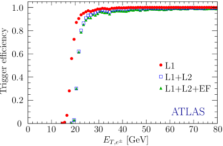
(b) Hadronic calorimeter
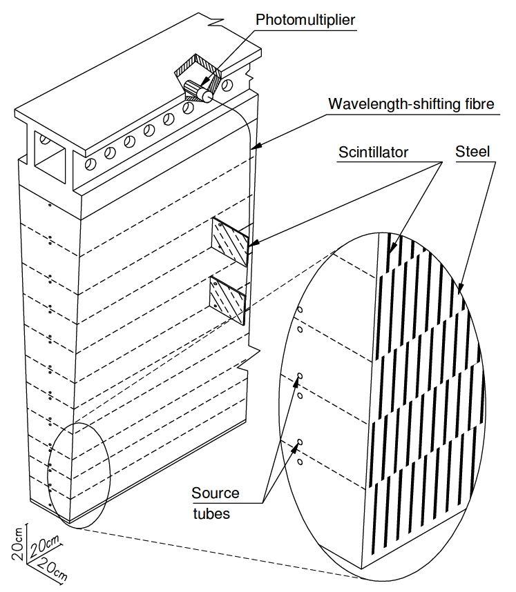
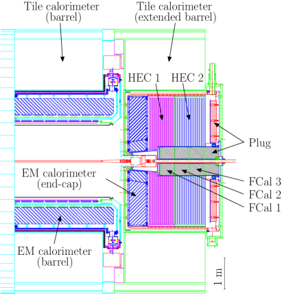

Technology.
The tile calorimeter is used in the barrel. It is a sampling calorimeter made of alternate layers of steel plates (absorbers) and scintillating tiles (active medium) orthogonal to the axis (Fig. 3.8.(a)). Ionising objects (hadrons or jets) as they pass through the tiles induce the production of ultra-violet scintillation light which is converted to visible light by wavelength-shifting fibres. The fibres are grouped together and coupled to photo-multipliers. Just like for the EM calorimeter the shape and energy of the object is measured as the object yields all its energy in form a shower.
Sampling calorimeter made of flat copper plates (absorber) and LAr (active medium) are used for the end-cap calorimeter while the forward calorimeter uses both LAr in association with copper and tungsten (absorbers).
Geometry.
The tile calorimeter (, , ) is made of one barrel (, ) and two extended barrels (, ).
In the forward pseudo-rapidity the hadronic end-cap (HEC) and forward calorimeter (FCal) are implemented to enhance the hermetic confinement of the produced particles to refine the measurement of (Fig. 3.8.b). The end-cap calorimeter (, , ) is split in a front wheel (HEC 1 : ) and a rear wheel (HEC 2 : ).
The forward calorimeter () measures the energy of the intense particles flux in this forward region, it is divided in three layers of equal length, first an electromagnetic and then two hadronic calorimeters. It relies on copper–LAr in the first layer (FCal 1) for electromagnetic calorimetry and on tungsten-LAr in the two last hadronic calorimeters (FCal 2 & 3).
The granularity in the barrel and extended barrels is of the order of and of in the forward calorimeters.
3.2.4 Muon system
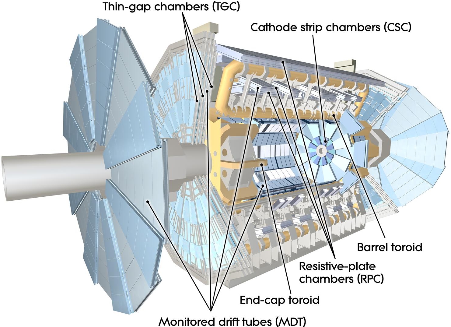
The muon precision tracking instruments and the toroidal magnet are reviewed. Information on the muon triggering relevant to the present analysis is given as well. An overview of the muon spectrometer can be seen in Fig. 3.9.
Technology.
The bending of the muons is done in the plan by a toroidal field which strength can reach in the barrel and in the end-cap. Nonetheless, the magnetic field bending power is characterised rather by its integral over the track length inside the tracking volume , where is an infinitesimal track portion. Large values of are necessary to make precise measurements of muon tracks.
Over most of the pseudo-rapidity range, precise measurement of the track coordinates in the principal bending direction is provided by Monitored Drift Tubes (MDT). As muons pass through a pressurized gas mixture filling the tubes, ionised electrons drift to the anode wire. The radius of the particle passage in the tube is deduced using space drift–time relation. Eventually, all collected radii give the muon track as shown in Fig. 3.10.(a).
For larger pseudo-rapidity, Cathode Strip Chambers (CSC), which are multiwire proportional chambers with cathodes segmented into strips, are used due to their higher rate capability and time resolution. Both cathodes are segmented. The one with strips orthogonal to the direction of the wires measure the precision coordinate, while the other with strips parallels to the wires provides the transverse coordinate. The position of the track is deduced by interpolating the charged induced among adjacent strips (Fig. 3.10.(b)).
The trigger chambers use Resistive Plate Chambers (RPC) in the barrel and Thin Gap Chambers (TGC) in the end-cap. In top of their triggering primer role, these chambers provides second coordinate measures in the bending plane to cross check the ones from the MDTs.
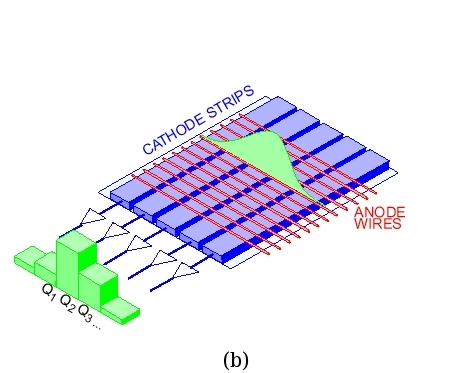
Geometry.
The magnetic field is generated in the barrel using three large air-core toroidal magnet (, , , ), each of them composed by eight coils arranged radially and symmetrically around the axis. In the end-cap two smaller magnets (, , , ) are inserted into both ends of the barrel toroid. In the transition region (), tracks deflection are done by a combination of both barrel and end-caps magnet field.
MDTs configuration follow a projective geometry and display a orientation of the wires in both barrel and end-cap. In the barrel, MDT chambers are arranged in three concentric cylindrical shells () around the beam axis at radii of approximately , and . In the end-cap they are confined inside large wheels () perpendicular to the axis at and . CSCs () are arranged in wheels with approximate radial orientation of the wires. RPCs and TGCs are respectively used in the barrel () and in the end-caps (), their implementation based on the one of the MDT and CSC modules. There are in total three layers of RPCs in the barrel and three layers of TGCs in the end-cap.
Trigger on muons.
Again, like for the electron the muon trigger efficiencies has already reached a plateau at where the data starts to enter the analysis (Fig. 3.11). Still here, contrary to the EMC, some asymmetries can arise between and due to the toroidal topology of the magnetic field which, for a given side of the detector, is in-bending for a charge and out-bending for the opposite charge. Nonetheless such effect should be mostly insignificant with respect to other apparatus limitations.
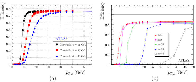
3.3 The ATLAS inner detector
3.3.1 Description of the inner detector
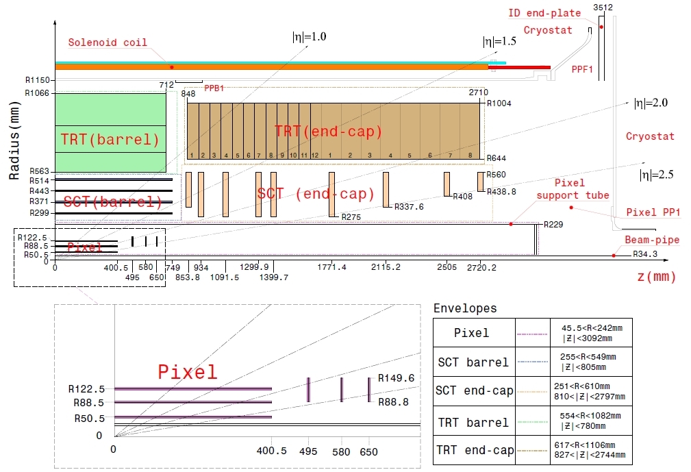
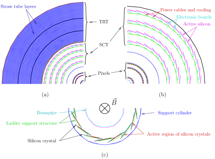
The ATLAS inner detector [96, 97, 98] pixel, SCT and TRT elements along with the central solenoid are described below. Their implementation is displayed with details on Figs. 3.12 and 3.13. Since the analysis strategy to decrease systematic errors relies on the possibility to invert the magnetic field of the solenoid, mentions on the drift of charge carriers in the modules were found worth to be noticed.
The Inner Detector is designed to provide a fine pattern recognition, an excellent momentum resolution and both primary and secondary vertex measurements for charged particles tracks displaying and within the pseudo-rapidity range . This is achieved by using three independent but complementary sub-detectors. At inner radii, high-resolution pattern recognition performances are done by discrete space-points from silicon pixel layers and stereo pairs of silicon micro-strip (SCT) layers. At larger radii the Transition Radiation Tracker (TRT), made of gaseous proportional counters embedded in radiator material, allows continuous track following. Each track leaves at least 7 hits in the precision tracking (pixel and SCT) and an average of hits in the TRT.
The central solenoid with the pixel, SCT and TRT detectors are now described.
(a) Central solenoid

The solenoid coil, surrounding the tracker, generates a magnetic field to bend the tracks of charged particles emerging from the interaction point allowing, with the tracker instruments, to identify and measure their transverse momenta.
The solenoid coil [100] (, ) provides a magnetic field
| (3.14) |
In that equation, is the main component of the field and the radial component , optimally null at , grows with due to border effects and the influence of iron in the tile calorimeter (Fig. 3.14). Charged particles are bent predominantly in the plane with bending powers of at decreasing to at . Besides, since the solenoid length is shorter than the tracker the field inhomogeneities in the forward region need to be accounted using a field map in both simulation and reconstruction.
One aspect in the present study relies on the capability of inverting the magnetic field of the solenoid which, although not programmed so far, is possible as stated in Ref. [100]. The consequences of this operation, from the physics analysis point of view, will be discussed in the analysis in Chapter 6.
(b) Pixel detector
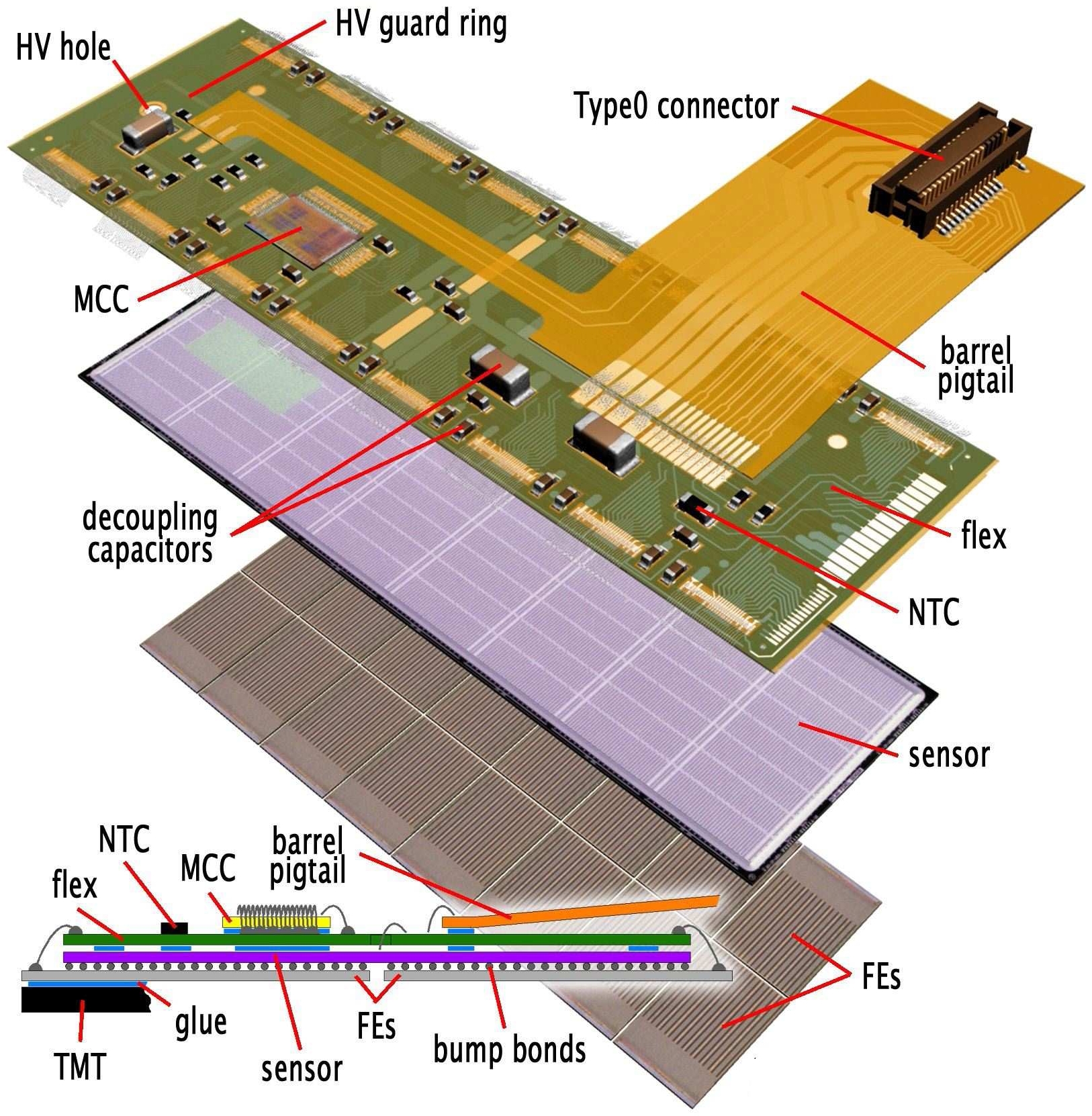
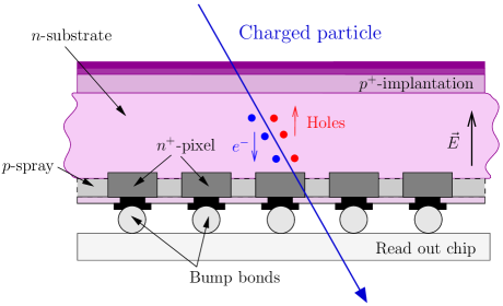

The measurements from the pixel detector [97] are fundamental as they provide information on charged particles before they yield energy to the apparatus. Silicon detectors are used to provide fine vertexes information with high granularity [101]. The cells are made, as shown on Fig. 3.15.(a), using silicon sensor layers of size segmented in both width and length to provide the pixel information. Incoming charged particles ionise pairs of electrons/holes in the silicon. The bias voltage applied in the silicon makes electrons drift to the -side readouts. Bump bonds transmit the collected charge to the front end electronic allowing to decipher which pixel was hit (Fig. 3.15.(b)).
Pixels modules –all identical in design– are dispatched between a central and two forwards parts. The central part is made of three concentric cylinders and the forward one are made each of three disks orthogonal to the axis. This provide for each particle track 3 hits.
In the central barrel, as can be seen in Fig. 3.13.(b), modules are tilted in with respect to the tangent position. This tilt provides an overlap of the active area of the modules in the -direction which enhance the hermetic confinement of particles. It also ensures a better spatial resolution via the alignment of the effective charge drift –induced by the field via Lorentz force– direction with the particle trajectory [102] as seen in Fig. 3.16.
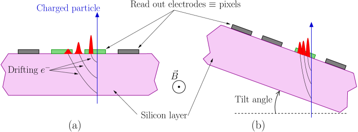
Layers are segmented like . In the forward barrel, that same segmentation correspondence is .
(c) Semi-Conductor tracker
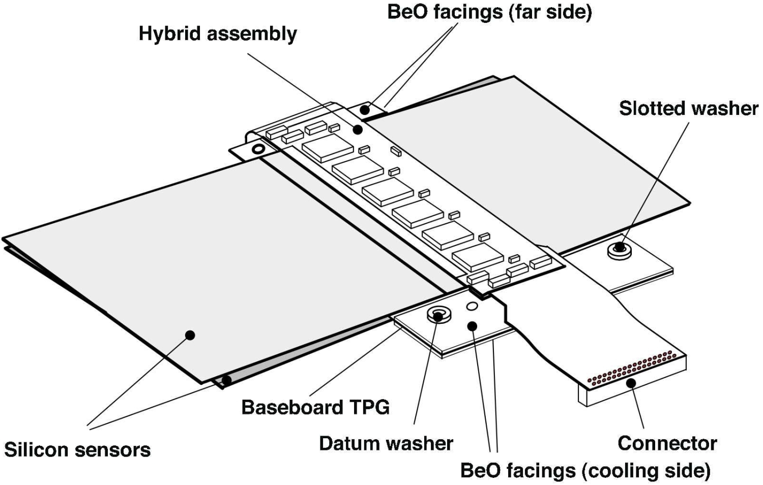
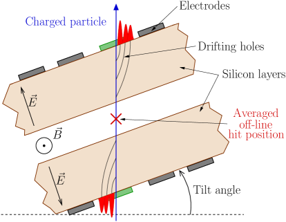

The SCT [97, 103] is based upon silicon micro-strip detector. Each module is made of two silicon sensor layers segmented in strips put back to back and rotated by 40 mrad to enhance the measurement (Fig. 3.17.(a)). The principle of operation is similar to pixel detector modules. Here the holes drift to the strips while the electrons drift to the back of the sensor. The strips are read out by a front-end chip, which measures the induction signal of the drifting holes/electrons pairs. Especially as shown on Fig. 3.17.(b) the Lorentz drift in each layer are working in opposite directions. The position of the hit is averaged offline from the two sides hit positions. The active area is and the modules are segmented in both width and length.
The layout is made of four layers in the barrel and of nine disks in the end-cap orthogonal to the direction. In the barrel modules are slightly tilted from the tangent position (Fig. 3.13.(b)) for the same reasons than for the pixel detector. The segmentation in the barrel is . In the end-cap, modules are also mounted to display some overlap and the corresponding segmentation is of .
(d) Transition radiation tracker
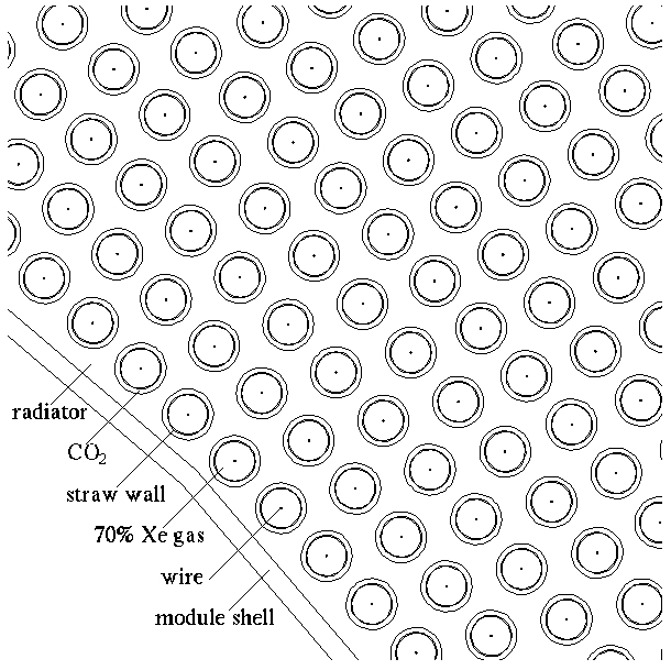
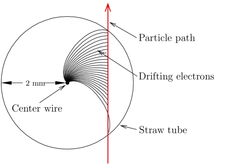

The TRT [97] assures continuous tracking as well as electrons identification. Even if it is not as precise as the silicon trackers its long lever arm plays an important role in the momentum resolution.
The TRT is made of layers of gas filled straws interleaved with transition radiation material. A charged particle passing through the straw ionise the electrons of the gas mixture (Fig. 3.18.(b)). A large potential difference is applied between the straw wall and the wire. The anode wire collects the energy of the ionised electrons (Fig. 3.18.(b)). Also, charged particles as they pass trough materials of different dielectric constant (radiator straw) radiate photons proportionally to their Lorentz factor. Part of the gas mixture in the straw is sensitive to photons and in consequence this ionisation energy adds up to the collection of the one induced by the incoming particle. The threshold for a significant radiation (), depends then on the mass of the particle and help to identify electrons amid other heavier charged particles. The TRT only provides information in with an accuracy of .
In the barrel the straws are parallel to the axis and arranged in three cylindrical rings. In each end-cap the wires are aligned to the radial direction and arranged in three sets of identical and independent wheels. Again the precise dimensions and pseudo-rapidity coverage can be seen in Figs. 3.12.
3.3.2 Track fitting and general performances
The track fitting is realised in three stages. First the raw data from the pixel/SCT and TRT detectors are respectively converted into clusters and calibrated circles. The SCT clusters are converted to space-points using a combination of the cluster from both sides of SCT modules (cf. Fig. 3.17.(b)). Then comes the track finding stage where algorithms [104, 96] essentially follow pattern recognition starting from the innermost pixel layers and goes outwards to the TRT. These algorithms, based on Kalman filter techniques [105] and Global- [106], perform recognition of helices among the hits in the tracker. In the final stage primary vertexes are resolved. Also tracking information from the muon spectrometer is used as well to enhance the data on muons. In the present work the expected stand-alone performances of the tracker are used exclusively.
The ID performances in , and can be parametrised using Gaussian functions (cf. Ref. [99] § 3.3.1.6) where, up to the approximation the material and the solenoid field are uniform in writes
| (3.15) | |||||
| (3.16) | |||||
| (3.17) |
where are in GeV and (true) superscript means a kinematic is considered at the generator level.
3.4 The weak modes affecting the inner detector
3.4.1 Misalignment and definition of the weak modes
The tracker is build into an a priori perfect “blue-print” configuration, but in reality modules assembly differs from such an ideal picture due to mounting limitations, mechanical stress, temperature variations, sagging due to gravity, etc. Since the tracker relies on the relative hits positions to measure the particles momenta and vertexes these small misalignment spoil the relevancy of reconstructed tracks. Since the module positions cannot be touched after their assembly modules misalignment are accounted by performing a mapping of the detector shape and module positions to correct the collected data. This procedure is called the alignment. Since some of the constraints on the tracker are time dependent this alignment survey must be continually updated.
The alignment of the tracker is realised using two kind of methods : hardware-based and track-based methods. Hardware methods make in situ measurement of the shape of the support structure and its change over time. Track based alignment requires, using the least squares principle, that the measurements in the detector are consistent with the assumed track model, i.e. follows the expected track trajectory in the given field and the scattering is consistent with the known amount of material.
Still, despite these surveys some deformations are such that the fitted track even if being relevant from the tracking algorithm point of view –i.e. an helix is recognised– nonetheless deviates from the real track. These deformations can be –in a first approximation– represented by a set of 9 simple and independent distortions called the weak modes [107], parametrised using global deformations on the tracker. Due to the symmetry of the problem, the parametrisation is made in the cylindrical coordinate system, hence the combination of deformations in , and directions folded with , and variations gives 9 weak modes. The total misalignment of the tracker is a combination of these 9 modes gathered in Fig. 3.19.
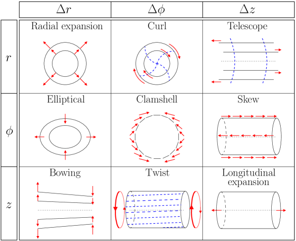
3.4.2 Consequences of the weak modes on the error on the W boson mass measurement
Curl and twists modes are responsible for limitations on the precision on the mass determination at CDF II [109]. In CDF II systematic errors on are of the same order than the statistical errors, i.e. while at the LHC statistical errors will be of the order of already for one year at low luminosity. For that reason the weak modes have to be addressed more thoroughly within ATLAS in regard of the difficulties encountered in the CDF II tracker (cf. Appendix 3.A). For example, considering again our interest in production, a requested precision of for the measurement of the constrains track parameters and momentum uncertainties. For that purpose the degradation of the high tracks parameters due to misalignment have to be smaller than while the systematic uncertainty on the momentum resolution needs to be smaller than [99, 110].
Here the focus is made on the predominant modes increasing the error of . Like it will be explained thoroughly in Chapter 5 the present work is based on the knowledge of the transverse momenta of charged leptons decaying from single bosons. Hence the attention is cast on modes affecting the reconstruction of positive and negative transverse tracks. Modes involving deformations are not considered as they do not degrade the resolution of , this leaves and modes which are discussed below. Two kind of biases are considered, the ones biasing the positive and negative charged particles tracks curvatures in the same direction (coherent biases) and the one affecting them in opposite directions (incoherent biases) the latter being the most important source of errors for . In what follows no values are estimated, only the relative qualitative amplitudes between coherent and incoherent biases.
The modes amplitudes biases are noted and tagged using the matrix form displayed in Fig. 3.19, i.e. using the notation or , or and or . The sign of a scalar is noted .

(a) modes
: radial.
The radial expansion () and contraction () infer coherent biases. This is shown in Fig. 3.20.(a) in the case of a radial expansion while starting with smeared curvatures of the same values . The reconstructed curvatures can be written in the first order of a perturbation expansion in the parameter that governs the radial expansion/contraction amplitude :
| (3.18) | |||||
| (3.19) |
: elliptical.
For this mode, the effect of the gravity will most likely flatten the tracker as depicted in Fig. 3.19. In the region where the nominal radius of the tracker is larger () positive and negative particle tracks curvature are overestimated. On the contrary tracks are getting more straight in regions where the tracker’s nominal radius decreases (). Eventually these two effects should compensate each other and leave a residual coherent bias such that .
: bowing.
Here, for a given coordinate positive and negative reconstructed tracks will be more straight (bent) if the tracker is expanding (contracting) with respect to its nominal radius. Biases coming from expansions are counter balanced by the one arising from contractions. The final bias from the bowing should be a residue from the averaging of these two opposite constraints. In any of those cases, again, the coherent bias should verify .
(b) modes
: curling.
The curling of the tracker gives incoherent biases. Figure 3.20.(b) shows it in the case where and with smeared curvatures are of the same values . The curling acts on the curvature like where is the bias induced by the curl. For small enough values of we assume –to keep the same parametrisation used up to now– that the reconstructed curvatures can be written in the first order of a perturbation expansion in the parameter governing the curl amplitude :
| (3.20) | |||||
| (3.21) |
: clam-shell.
This mode is unlikely to affect any component of the inner tracker [111].
: twist.
To illustrate the twist, a rotation of the tracker of the left side and of on the right side are considered. Based on the understanding of the curl mode, on the left side positive tracks are believed to be more bent while negative tracks are believed to be more straight. On the right side this effect is reversed. Just like for the bowing, antagonists modes of the same amplitudes cancel each other. Eventually the most important twist should contribute with a term like .
(c) Global effect of the 6 previous modes
In conclusion, the reconstructed positively and negatively charged tracks should be biased like
| (3.22) | |||||
| (3.23) |
where and are respectively the global coherent bias from and modes, i.e.
| (3.24) | |||||
| (3.25) |
Again, let us repeat that only qualitative estimations are made here. This is justified as in our work these biases will be implemented with large worst case scenario values to improve the robustness of our proposed analysis scheme.
Appendix 3.A W mass charge asymmetry and tracker misalignment in CDF II
(About the difficulties to measure because of tracker misalignment)
“You all remember how during your studies you were taught a solid could be described by only six degrees of freedom. Well. Forget about it. It’s crap.”CTEQ-MCnet Summer School 2008 - Standard Model lectures
Tom LeCompte
3.A.1 Context of the measurement of the W mass at CDF
The CDF detector used in Tevatron Run II, labeled CDF II [109], is a multipurpose detector nominally forward-backward symmetric with respect to the interaction point where protons and anti-protons collide at a center of mass energy of . It is made, starting from the beam-pipe, of an inner tracker bathing in a solenoidal magnetic field, an electromagnetic calorimeter followed by a hadronic calorimeter to contain and measure respectively the energies of electrons/photons and hadrons. Finally a muon spectrometer surrounds the previous apparatus to measure the properties of muons. The data is read-out on-line using the decisions of a three level trigger system.
The measurement of [51, 56] in CDF II is achieved using the tracker data for the muons and both tracker and electromagnetic calorimeter data for electrons. The acceptance and resolutions for central electrons and muons are the same which means both channels enter with the same weight in the analysis.
The extraction of is addressed via the usual observables such as , and and via muon and electronic decays of the . Along all these information the difference between the masses of the positive and negative bosons is estimated as a mean of consistency check. Actually this last measurement is not to be apprehended as a real attempt to measure . Rather than that is has to be understood that the measurement is entirely focused on and that the effects responsible for the low precision on were at no time addressed by the authors as long at it does not have a major role for the determination of . Both and CDF results for these last years, as seen in Table 2.2, are recaptured here :
| Channel | [] | [] | Year | ||
|---|---|---|---|---|---|
| 1990,1991 [52, 53] | |||||
| 1995 [54, 55] | |||||
| 2007 [56, 51] | |||||
The question one might ask is how come the absolute mass is measured with an error of then ? The trick is that incoherent biases are at work between the positively and negatively charged particle tracks and they get drastically reduced when both charges are merged.
The next subsection describes briefly the CDF II central outer tracker used for the measurement. After that a recapitulation of how the tracker misalignment affects charged particles curvature is made. This shows how the experience from Tevatron physicists guided us to address, aware of the LHC/ATLAS original features, the relevant weak modes for a future dedicated measurement of in ATLAS. It also explains why so far all experimental measurements of display such a low accuracy.
3.A.2 Description of the CDF Central Outer Tracker
The CDF configuration is such that we borrow for its description the same conventions adopted for ATLAS (cf. § 2.3). The CDF II uses silicon at lower radii and drift tubes technologies afterward. The silicon detector is not detailed since its data was not used for the determination of .
Around the silicon tracker is an open-cell drift chamber, the COT [112] which span the radial range and extend longitudinally for ().
The COT, as displayed in Fig. 3.21.(a) is made of eight concentric “super-layers” separated in azimuth into cells. Each cell, as shown in Fig. 3.21.(b), is made of sense wires and potential wires immersed in an ambient gas mixture. Ionised electrons from the passage of high energy charged particles drift under the influence of the electrostatic field to the sense wires and yield their energy which allow to decipher the particle hit position. The sense wires are attached at each extremities to end-plates which hold them into a string position. The tilt angle of the cells aims to make it so the ionised electrons travels approximately in azimuth to the sense wires under the combined influence of the solenoid magnetic field and of the local electrostatic field. Let us note that the cells move from their nominal geometry under the influence of gravity which makes field sheets and wires sag. This eventually implies that the sense wires deflect toward a particular field sheet. To decrease this effect a support rod at connects the sense wires at the center of the detector.

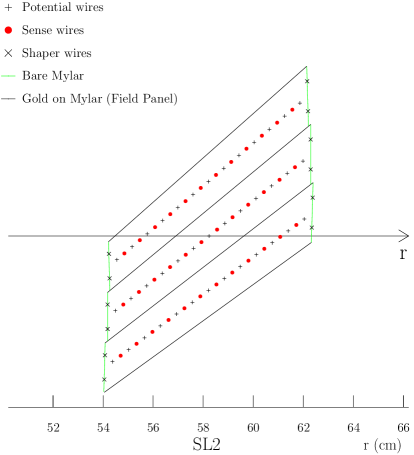

3.A.3 Influence of tracker misalignment on the W mass charge asymmetry
We adopt in the rest of this Appendix the conventions of Ref. [51] to address the curvature of a charged particle track in the plane. It is defined like
| (3.26) |
where is the charge of the particle and is the radius of the track in the plan. Charged leptons have their transverse momenta deduced from which is measured by the hits left in the COT. For that purpose the position of the cells needs to be determined precisely to have a good accuracy for the momentum scale. The calibration of this momentum scale is determined starting with the a priori position of the cells. Then in situ measures correct for the electrostatic and gravity sag biases, cosmic ray muon data allow to add up in situ corrections and finally track based corrections are applied using data calibration. For these last corrections first comes the study to reduce relative curvatures biases between positive and negative particles and finally absolute scale data calibration using , and bosons decays to .
The reconstructed track curvature can be expressed as a function of the true curvature in a Taylor expansion around zero which is justified by the high of the charged leptons of interest (). It reads
| (3.27) |
which now allows us to consider the case of two positively and negatively charged leptons respectively of curvatures and , having the same true transverse momentum (i.e. ). Their reconstructed tracks are written
| (3.28) | |||||
| (3.29) |
Now, remembering the goal is to eventually merge positive and negative channels for the extraction of , flipping the sign of the curvature in Eq. (3.29) (i.e. ) to get rid of the charge sign and averaging this new expression with Eq. (3.28) gives an average track curvature
| (3.30) |
With that development we see all terms of even power of are cancelled when averaging, the term linear in scales the true curvature and is deduced from momentum calibration. The term is the first one to affect the determination of but it can be neglected because of the high transverse momentum of the leptons. On the other hand, the direct average of the signed curvatures (Eqs. (3.28–3.29)) that should ideally be equal to zero, leads to constraints on , indeed
| (3.31) | |||||
| (3.32) |
where in the last line higher order terms are neglected compared to and because as we saw they are not worth to be considered for a measurement of . Then, is constrained using data calibration since the relative difference between should be zero in the absence of misalignment. The parametrisation of Eq. (3.32) can be written like
| (3.33) |
where the terms , and can be interpreted as distortions of the COT.
Figure 3.22 illustrates these distortions as a function of the more intuitive observable. Using the vocabulary of weak modes (cf. § 3.4), the term in corresponds to a curl of the tracker while the term corresponds to a twist between the left and right end-plates. The term proportional to goes beyond the first order approximation of the weak modes and is characteristic of the COT construction, it corresponds to a curl of second order where the left and right end-plates are being rotated in the same direction but the center of the tracker is maintained to its original position by the support rod. The terms in and corresponds to mis-measurements of the beam position.
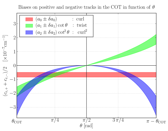
Figure 3.23 shows now the tracker misalignment consequences on before and after corrections in function of .
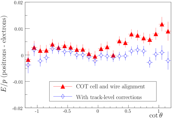
In conclusion, this measurement dedicated to extract merges both and measurement which gives data where half of the tracks are biased in one direction and the over half of the same amount but in the opposite direction. Eventually all those corrections lead to a precision on tracker momentum resolution of which in turn leads for all , and fits to a systematic error of for the measurement of . But, when performing fit analysis for separated and the curl distortion ( and ) give rise as it was seen in the core the Chapter to incoherent biases between the positively and negatively charged tracks curvature responsible for the important difference of the order of . From that experience we can state that the LHC capabilities and a dedicated measurement strategy should considerably improve the accuracy on the value .
Chapter 4 The Monte Carlo event generator WINHAC
veillant
doutant
roulant
brillant et méditant
avant de s’arrêter
à quelque point dernier qui le sacre
Toute Pensée emets un Coup de DésUn coup de dés jamais n’abolira le hasard
Stéphane Mallarmé
So far a description of the theoretical and experimental context in which the prospect for a measurement of have been given. This Chapter describes the tools that were used for that purpose, which consist mostly of a description of the Monte Carlo event generator WINHAC used to simulate the production of bosons in Drell–Yan. The other tools entering in the generation and the analysis steps are also described briefly.
This Chapter is divided into three parts. The first one, after reminding the gist of Monte Carlo methods, describes the physics implemented inside WINHAC. The second part presents the work done within this thesis to implement WINHAC inside the ATLAS software. The reader interested only in the physics thread can skip this technical part in a first reading. Indeed, to the use of the full and refine ATLAS software, a lighter framework was preferred to make the studies presented in Chapter 5 and 6. This personal framework is eventually presented in the third part of the Chapter.
4.1 The Monte Carlo event generator WINHAC
4.1.1 Monte Carlo methods
Monte Carlo (MC) methods [113] provide in high energy physics efficient solutions to deal with numerical integration and, due to their very stochastic nature, to simulate inelastic scatterings for both phenomenological and experimental specific needs. The principles of MC procedure is reviewed in a nutshell.
(a) Principle of Monte Carlo methods.
Starting with one dimension, the numerical integration of a function between and can be recast as the product of the integration range by the average of the integrand over it, that is
| (4.1) | |||||
| (4.2) |
This last expression can be approximated using a discrete number of points within the range , giving then
| (4.3) |
Two types of methods can be distinguished to evaluate . The first one consists essentially to slice regularly the integration range, these are called numerical quadratures. A broad range of refinements exist to increase the accuracy and convergence speed of the result (see e.g. [114]). Among them let us mention the trapezium and the Simpson rules which accuracies in one dimension are respectively converging like and . The second approach consists to pick up random points in to approximate . This is the principle of Monte Carlo procedure, which in the one dimension case display a convergence .
When the dimension of the integral increases to a higher dimension, say , quadrature integration methods become very cumbersome as the integration volume, or phase space to already adopt physics vocabulary, needs to be split into bits. Thus, the trapezium and Simpson methods converge now like and whereas for the MC integration by still picking up random points in the phase space keeps a convergence . Then, Monte Carlo may be slow but their speed convergence is independent of the dimension of the integral.
Since at the LHC the typical number of produced particles in an inelastic scattering is of the order of it implies a dimension where the subtraction of to the degrees of freedom is a consequence of the energy/momentum conservation.
(b) Monte Carlo in High Energy Physics.
Coming back to high energy physics, estimating the probability of occurrence of a LHC reaction demands the computation of its cross section which can be roughly written
| (4.4) |
where is an infinitesimal element of the phase space of the process and is calculated with perturbative QCD/EW/BSM along with the relevant and available higher corrections depending on the nature of the process. Let us emphasise that here, picking up a random element corresponds to a particular physical configuration for the event, that is four-momenta of the colliding partons, of the decaying particles as well as other partons and photons which have been radiated. Hence, the record of these random elements, in top of helping to compute , represents a collection of events which can be kept and used to plot afterward any desired distribution for an observable in the form . Note this would not be possible with quadrature procedures where from the start the calculus should be aimed to resolve a particular distribution. This collected events are referred to as “weighted events” as they are indeed weighted by the theoretical prediction associated to their production.
Nonetheless, these weighted events are not a simulation of real physics processes. Indeed in nature a physical event do not come with the information whether it is frequent or rare, only harvesting large enough data allows to see it. Still, from the simulation of weighted events a simple trick can be used to emulate the outcome of unweighted events, that is events with a weight of . The principle is the following. In a local region of phase space a maximum is determined for the integrand, i.e. . When a weighted event is generated a random number is draw in the range then
-
-
If the event is accepted with a weight of .
-
-
If the event is simply rejected.
This rejection method allows to produce events with the same frequency of occurrence than in reality. Histograms produced with weighted and unweighted events are the same in the asymptotic limit (in practice when is large enough so the Central Limit Theorem can be applied). Let us note this trick is possible because the integrand is positive definite which is true only at LO in QCD, the QCD NLO treatment becomes then very delicate , e.g. Ref. [115].
Monte Carlo event generators opens, from the experimentalist point of view, a wide range of possibilities. During the generation, acceptance cuts as well as detector smearing on the generator predictions can be applied which justify their extensive use in both R&D prospects and real data analysis.
Also, worth mentioning is the generation of random numbers. It is impossible for an algorithm to generate random numbers since, by definition, its behaviour is deterministic by essence. Hence random numbers are in fact sequence of pseudo-random numbers outgoing small algorithms. The quality of these sequence of number comes from their periodicity –the time it takes to repeat the series– and some short-range correlations between the generated numbers (see e.g. Ref. [116]). To better emulate the non correlation between several simulated data, different long sequences can be generated using different seeds in the algorithm initialisation. In the rest, for convenience, the term random is used instead of pseudo-random.
We can distinguish two types of Monte Carlo, the one using the MC technique only for integration and the other which profit of MC properties to simulate physics processes. The latter are referred to as “event generator” or simply “generators”.
Another way to classify Monte Carlo, from the physics point of view this times, is to look at their domain of applications. On the one hand stands a few general purpose MC that possess a wide range of inelastic scattering ( or ) implemented for both SM and some BSM processes. They also provide the radiation of photons from leptons and photons/gluons from quarks (called in that context QCD “parton shower”), the hadronisation of jets, decays of unstable particles and the underlying event. The most frequently used general purpose MC are Pythia [117, 118, 119], Herwig++ [120, 121] and Sherpa [122, 123]. The other category are MC focused on specific processes but that embrace more corrections at the level of the hard process () compared to the general purpose MC. To obtain eventually physical events just like the one we observe in experiments they are interfaced to general purpose MC. These tools are quite numerous and span large domains of physics, this can go from standard processes with higher QCD/EW corrections to the supply of corrections to existing MC events such as higher QED radiation in the final state like PHOTOS [124, 125, 126] or management of or Higgs decays done respectively by TAUOLA [127, 128, 129] and HDECAY [130].
The refinements brought to the art of MC integration and event generation in High Energy Physics goes far beyond the short overview made here. Among them is the variance reduction to improve convergence speed, the handling of singularities in the integrand, and the delicate issue to generate events at NLO in QCD. All those points and many others are addressed in dedicated documents.
There is, so far, no classic textbooks on the use of MC techniques in high energy physics. Nonetheless, the reader eager to learn more on the subject is invited to look at the thesis of Michael Seymour [131] where one chapter provides a short yet thorough description of the matter. Other relevant sources are the presentations given by Monte Carlo experts in conferences (see e.g. [132, 133, 134, 135, 136]).
(c) Weakness of Monte Carlo methods.
So far Monte Carlo methods have been promoted as the best tools one can work with in experimental high energy physics. Nonetheless, to be completely objective some light is cast on a few of their weaknesses.
The use of Monte Carlo simulation are safe when it comes to pragmatic application. To illustrate this let us consider the example of nuclear safety where the control of the behaviour of a nuclear facility relies on Monte Carlo simulations. In no case the underlying model implemented have to be perfect, as long as it sticks to physical measurements. Then, using phenomenological models altogether with empirical laws are correct as long as the intended goal –the control of the facility– is assured.
In high energy physics the aim is different. MC generators are introduced to simulate known processes but as well to help unravel possible deviations in paradigm models or even discover brand new processes. Now the actual models are far from being perfect, large parts describing inelastic scatterings are modeled by non perturbative QCD, which relies on complex –and sometime empirical– parametrisation (e.g. hadronisation). This poses a problem for the relevancy of an experimental analysis.
The awareness of these imperfection’s acted as an incentive in the present work to come up with analysis strategies which had to adapt to a given measurement to get as much as independent from MC imperfections. Also, in a first step, rather than using several Monte Carlo the choice for a deeper understanding of the used tool, WINHAC was adopted this being justified by the latter strategy to make an analysis.
To conclude with this parenthesis, some quotations on this particular topic. The first one is extracted from a talk by J.D. Bjorken [137] as noted by Torbjörn Sjöstrand in [115]
“The Monte Carlo simulation has become the major means of visualization of not only detector performance but also of physics phenomena. So far so good. But it often happens that the physics simulations provided by the Monte Carlo generators carry the authority of data itself. They look like data and feel like data, and if one is not careful they are accepted as if they were data.”
The second one is from the authors of Pythia who warn the users about the traps one can fall into
You must be very careful when you formulate the questions : any ambiguities will corrupt the reply you get. And you must be even more careful not to misinterpret the answers ; in particular not to pick the interpretation that suits you before considering the alternatives. Finally […] the current authors might unwittingly let a bug free in the program Pythia.
In conclusion a warning from the authors of Ref. [138]
Monte Carlo event generators are complicated programs that will almost inevitably contain bugs, incorrect assumptions and ill-chosen parameters. It is therefore vital that a user does not take any results at face value. As a minimum at least two completely independent programs should be used in any physics studies.
4.1.2 The Monte Carlo event generator WINHAC
The main tool that used in the present study is the Monte Carlo event generator WINHAC [139, 140, 141, 142]. It has been developed in FORTRAN 77 (F77) by Wiesław Płaczek and Stanisław Jadach from the Cracow theoretical group which holds a leading role in term of electroweak radiative corrections in Monte Carlo.
WINHAC is dedicated to precision description of the charged-current Drell–Yan process. It has been thoroughly tested and cross-checked with independent calculations [139, 140, 143, 142]. This MC program has already been used in previous studies of experimental prospects for exploring the electroweak symmetry breaking mechanism [144], in our ongoing effort for precision measurement of the Standard Model parameters at the LHC within the ATLAS experiment [145, 146, 72, 74].
At the time of the redaction of this dissertation, the most recent version of WINHAC is release 1.30 [147]. It features the exclusive Yennie–Frautschi–Suura exponentiation [148] of QED effects, i.e. the radiation of photons in the final state
| (4.5) |
with , also referred to as multi-photon radiation. It also includes electroweak corrections for the full charged-current Drell–Yan process at the parton level, for more details see Ref. [142]. This parton-level process is convoluted with the parton distribution functions (PDFs) provided by the LHAPDF package [149] which includes a large set of recent PDF parametrisation by several groups. WINHAC is also interfaced with the Pythia 6.4 [117] MC event generator for the QCD/QED initial-state parton shower as well as for the hadronisation. Technical detail, Pythia and WINHAC are accessing to LHAPDF density functions through the LHAGLUE interface –present in LHAPDF– which mimics the procedure that was used formerly to use PDFLIB [150] the ancestor of LHAPDF. Several type of collisions are made available : proton–proton, proton–anti-proton, proton–ion, ion–ion, where each ion beam is defined by its charge number , atomic number and energy in the center of mass. For , the nuclear shadowing effects from Refs. [151, 152] can be optionally switched on.
The parton-level matrix elements are calculated numerically from spin amplitudes [139]. This allows for studies of any spin effects in the charged-current Drell–Yan process. In fact, WINHAC provides options for generation of processes with pure transversely or pure longitudinally polarised bosons at the Born level.
In addition to the charged-current Drell–Yan process, WINHAC includes the neutral-current Drell–Yan process (with bosons in the intermediate state), however at the Born level only. For precision description of this latter process, similar to the former one, a dedicated MC event generator called ZINHAC [153] is being developed in C++ by Wiesław Płaczek and Andrzej Siódmok. In the future, these twin MC generators can be used for precision studies/analyses of the Drell–Yan processes including the QED/EW corrections.
The generation of random numbers in WINHAC is achieved using different classic algorithms. The one used for our work is RANMAR [154, 155] which displays a periodicity of .
For this study version 1.23 of WINHAC has been used which for all aspects investigated and adopted strategies is equivalent to the latest version. They differ in description of QED/EW corrections but these have not been included in the present work. In Appendix 4.A an example of a WINHAC summary event is given.
As conclusion, in Table 4.1 we stress the place of WINHAC with respect to multi-purpose and a few specialised Monte Carlo that can produce or in Drell–Yan. In this table MC event generator (Event Gen.) are distinguished from the one using only MC as a mean of integration (Histograms). As it can be seen there is up to this date (2009) no Monte Carlo which hold QCD and EW corrections at the same level of detail.
| Monte Carlo | Refs. | Process | QCD | EW | Type |
|---|---|---|---|---|---|
| WINHAC | [139, 147] | , impr. LO | +QED FSR | Event Gen. | |
| HORACE | [156, 157] | , | , impr. LO | +QED PS | Event Gen. |
| Pythia | [117, 119] | , | , impr. LO | LO | Event Gen. |
| HERWIG | [158, 159] | , | , impr. LO | LO | Event Gen. |
| Herwig++ | [120, 121] | , | , NLO | LO | Event Gen. |
| Sherpa | [122, 123] | , | , impr. LO | LO | Event Gen. |
| MC@NLO | [160, 161] | , | parton shower, NLO | LO | Event Gen. |
| AcerMC | [162, 163] | , | , LO | LO | Event Gen. |
| ResBos-A | [164, 165] | , | , NLO | FS | Histograms |
| ResBos | [166, 167] | , | , NLO | LO | Histograms |
| WGRAD | [63, 168] | , LO | Histograms | ||
| ZGRAD2 | [169, 170] | , LO | Histograms | ||
| SANC | [171, 172] | , | , LO | Histograms |
Hence so far, Monte Carlo are usually combined to simulate with the closest possible accuracy the physics observables needed to be confronted to the data. For example the extraction of for the CDF II run [51] is made using the following Monte Carlo
- -
-
-
The photon radiation corrections in the final state are made by WGRAD [63] and correct the , and distributions from ResBos.
-
-
The background to ( and ) and to ( and ) are simulated using Pythia v 6.129 and passed to a GEANT-based full simulation of the detector.
4.2 Implementation of WINHAC in the ATLAS software
4.2.1 Introduction
This part of the Chapter covers the work achieved in the context of this thesis to implement WINHAC in the ATLAS software environment.
As seen previously each detector needs, for both R&D and data analysis, to have at its disposition different Monte Carlo event generators to simulate the physics to be studied. Their implementation needs to follow codified rules, just like any other tools in the experiment software, for clarity’s sake. On the one hand most event generators obey to custom rules and conventions and can be implemented in any programming language like F77, C/C++, etc. On the other, for convenience reasons, experiments software environment relies on automated skeletons that treat all the present generators with the same manner. For instance, Monte Carlo events needs, among many other things, to be smeared to simulate the particle interactions with the material of the detector. This simulation takes as input a standard data format which is completely blind to the generator that produced it. This example gives an idea of how a generator needs to fulfill a few requirements imposed by the experiment.
This section is divided as follow. After an overview of the main features of Athena [174], the software environment of ATLAS, follows a description of the context in which WINHAC was introduced, that is in the simulation and reconstruction chain of the Monte Carlo events inside ATLAS. The section ends on the implementation of WINHAC and the validation of this work.
4.2.2 Software environment of the ATLAS experiment
To better visualise the context of our discussion a brief overview of the software environment ATLAS relies on is given.
First of all, let us note the quantity of events selected by ATLAS together with the data outgoing their analysis should represents each year a volume of information of the order of Peta-byte111.. Hence to overcome this challenge ATLAS had to aim for a highly decentralised storage and data management. This system obeys to a certain hierarchy where tasks are split into facilities called Tiers which principal activities are recaptured below.
Although it will not be emphasised later on let us note that one of the philosophy in the use of Tiers prescribes, for obvious safety reasons, to make a least one back up of each data batch. The first data processing occurs at CERN in the unique Tier-0 facility where raw data are saved and reconstructed into ESD, AOD and TAG formats which description are gathered at the end of § 4.2.3. This first data batch are shared among Tiers-1, of the order of ten all other the world. The tenth of these raw data are stored to give new ESD, AOD and TAG. Tiers-1 need to provide good accessibility for the data they store as well as the necessary capacity to analyse them. Tiers-2 provide work related to the calibration, the simulation and the analysis. Finally Tiers-3 are made of local sources in each institute necessary to store custom data (e.g. ntuple) and act as well as access points to upstream Tiers. More details on the precise role of each Tier are given in Ref. [174]. This decentralisation of data processing and storage is provided by the Grid which allows to make out of the ATLAS software a virtual facility split between several calculators spread throughout the world.
The informatics environment of ATLAS is called Athena [174, 175]. Athena is an evolved version of the Gaudi [176, 177] framework developed initially by the LHC [87] experiment and is now common to both ATLAS and LHC projects. Amid the important features of Athena is the clear separation between the data and the algorithms as well as between transient data (in memory) and persistent (in file) data. The processing of the data for data selection, event simulation, reconstruction and analysis is governed by Athena. Athena is object oriented (OO). Its structure is build mainly in C++, uses extensively the ROOT System[178, 179] with some tools written in FORTRAN 77 or Java while the user interacts with Athena via Python.
4.2.3 Simulation and reconstruction of Monte Carlo events within ATLAS
Here we give a description of the different steps that allow, starting from Monte Carlo events or from real data, to reach reconstructed data. The first overview and the details that follow can be grasped looking at Fig. 4.1. Let us remind more details on the data type mentioned are compiled at the end of this section.
(a) Overview of the simulation and of the reconstruction
Starting with the real data. The event filter –the last process of the ATLAS trigger– provides as outputs raw data in byte stream format, i.e. sequence of /. These information are then converted to objects, the Raw Data Object (RDO) transmitted in turn to reconstruction algorithms. Before describing the reconstruction chain, let us come back to the stages the simulated data must follow. In the first step physical events are produced by Monte Carlo event generators, at this stage acceptance cuts can be applied on some observables such as , , , etc. These events, as seen previously in § 2.3, are labelled “truth events” or “generator level” data. They are transmitted to algorithms that simulate their passage in the ATLAS detector. This step is by far the most CPU time consuming. The output are hits, that can be merged with pile-up events, the latter receiving a special treatment. After comes the digitisation which goal is to emulate the electronic read-out chain of the several sub-detectors of ATLAS. This gives eventually simulated RDO. The simulation step finished the reconstruction chain is over-viewed.
Even though RDO are oriented object they are nonetheless raw data. Also the goal of the reconstruction, as its name indicates, consists to reconstruct objects containing only relevant information for a physic analysis.
Finally let us mention the fast simulation of the detector. Since the simulation part is very time consuming most experiments have tools with an approximated but faster simulation of the detector. In ATLAS, this fast simulation is called Atlfast [180, 181, 182]. It shortcuts all simulation chain steps, that is from the particles four-momentum outgoing the generator it directly gives reconstructed data.
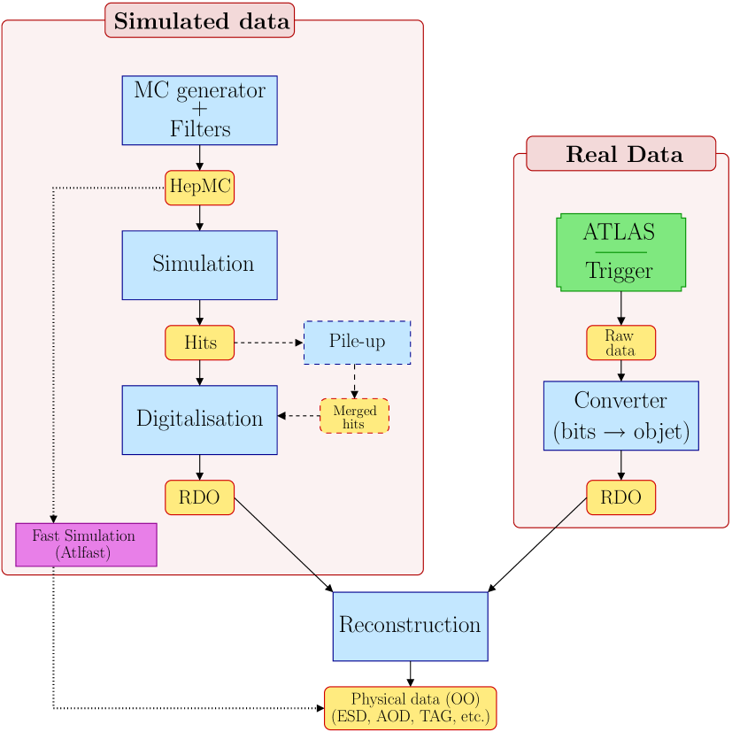
In the rest complementary information on the simulation and reconstruction chains are given. For each step the emphasis is made first on physics aspects and then on technical aspects. For further details on all technical aspects related to the Athena framework the reader is sent back to the ATLAS Computing TDR [174] and to the on-line workbook [175].
(b) The simulation chain
Generation.
The physics motivation being already known we move on directly to technical aspects with more emphasis with respect to other steps since the work for implementing WINHAC occurred at this stage.
Inserting a MC within ATLAS consists to write inside Athena a C++ interface calling the algorithms of the generator within its original libraries. Those instances are roughly :
-
-
The initialisation, which essentially switches on the MC generator algorithms, read the input parameters, etc.
-
-
The event loop in which the MC generate events.
-
-
The finalisation where algorithms are shut down and the data are saved.
These three steps are realised for all the generators within Athena via the inheritance of the methods of the class GenzModule.
Concerning the libraries of the stand-alone code they are stored outside of the Athena framework in AFS or in the GENSER (GENerator SERvice) repository. The goal would be eventually to maintain all generators libraries by the GENSER LCG project [183] which would provide validated libraries for the needs of both theoreticians and experiments associated to the LHC.
The random numbers in Athena are provided by the use of the Athena Random Generator Service which uses RanecuEngine [154] maintained by CLHEP [184].
The parton distributions functions are provided by the LHAPDF package [149].
The output for the events is in the HepMC [185] format that records information related to each event. The HepMC format possess an infinite number of entries, the storage of the matrix density in each vertexes, the flow pattern (e.g. color) and their follow up, the record of the used random numbers along with an arbitrary number of statistical weight that can be associated to each event. This tool developed in C++ by ATLAS members has become the standard for the record of high energy event and is now maintained by CLHEP.
Simulation.
The goal of the simulation stage is to simulate the passage of particles generated by the MC within the sub-detectors of ATLAS, i.e. energy deposit in the calorimetry and tracks left in both inner tracker and muon spectrometer.
This task is made by GEANT 4 [186, 187]. GEANT model the geometry and composition of the ATLAS detector, and simulate the physical process occurring as particles pass through each cells. Hits record information related to the position, yielded energies, identifications of activated elements, etc. For the pile-up Athena provides a stock of simulated pile-up and select for each event one random set and optionally merges it to the process simulated upstream.
Digitisation.
Hits need to be converted into an output of the same format with the one provided by the ATLAS detector for real data. For that purpose matters such as the propagation of charges (e.g. in the tracker or in the LAr) and of light (e.g. in the tiles of the hadronic calorimeter) as well as the response of the read out electronic needs to be emulated.
Contrary to the previous steps these tasks are very specific to the detector and cannot be accomplished without the physicist directly involved with the assembly and testing of each ATLAS specific sub-detectors. This step provides output in RDO format. Let us note all Monte Carlo truth information, kept so far for cross check, are removed from simulated RDO so that they exactly look like the format of the real data selected by the ATLAS trigger.
(c) Reconstruction of physic events
The goal of the reconstruction is to devise from raw data the vital information necessary to perform an analysis. To be more specific information related to photons, electrons, muons, taus, , jets, , primary vertexes, etc. These collected data from each sub-detector are combined to optimally reconstruct four-momenta for the widest range of momentum, pseudo-rapidity and whatever value of the luminosity, all of that with the less background for particle identification.
The reconstruction is split in several steps depicted in Fig. 4.2. In a first stage is the individual reconstruction of the data outgoing the sub-detectors (tracking and calorimetry) then comes the combined reconstruction which corresponds to the beginning of particle identification. An example of this step has been given for the case of the inner detector tracks reconstruction in Chapter 3 § 3.3.2. The output of this procedure are in ESD format.
In the second stage the preparation to the analysis starts with more complex reconstructed objects (e.g. -tagging) and with a reduction of the data to the AOD format.
Finally data are tagged with the use of TAG files created from the AOD.

(d) Sum up of the different data format
As seen previously different data format exist at different stages of the simulation and reconstruction chain. The list below makes a summary of the one mentioned earlier.
Raw data.
These are the data provided by the event filter, the last stage of the ATLAS trigger, and are written in byte stream format. Each file contains the information related to a run and each event, delivered at a frequency of , should weight . This data format, contrary to the one that follow, is not object oriented.
Raw Data Object (RDO).
The RDO is essentially an oriented object (C++) representation of the byte stream information from the raw data.
HepMC.
Format holding generator level information coming from MC generators, that is a purely theoretical information.
Hits.
Format carrying recording real interactions of simulated particles with the detector. Hits carry information like position, energy deposit, identifier of the active element, etc. after simulating the theoretical events in the ATLAS detector.
Event Summary Data (ESD).
These files contain reconstructed information necessary to deduce the identification of particles, the track refitting, the jet calibration, etc. The goal of this format is to avoid to access to raw data for every study out of the calibration context or of the re-reconstruction. Those files are written in POOL ROOT format [178, 179] with an average size of per event.
Analysis Object Data (AOD).
These POOL ROOT files are derived from ESD. They contain physical objects with information relevant to an analysis. It is on this format that in the long run most physical studies should be based upon. Each even takes a size on disk of the order of .
TAG.
These files are created in the goal to identify and select produced data. They contain information on the data batches, each event occupy a size of .
For conclusion several tests that were carried in this work to validate the implementation of the WINHAC interface are based on the CBNT (ComBined NTuple) format which hold data in Trees and leaves ROOT format.
4.2.4 Implementation of WINHAC inside Athena
(a) The Winhac_i interface
In this part we present Winhac_i, the interface between WINHAC and Athena. This work has been made in collaboration with Giorgos Stavropoulos to make of WINHAC an ATLAS approved Monte Carlo event generator used for the production of event samples as reported in Ref. [71].
The requirements from the Athena framework imposed to switch to its own random generator and to the use of the LHAPDF libraries since in the version of WINHAC used at that time (v 1.21) PDFLIB was still use. The feedback to the authors allowed the code to evolve in later releases to use of LHAPDF as the default option (v 1.22 and upper). Finally always at the time of this implementation the LHAPDF package did not provided nuclear corrections necessary when studying ion-ion collisions. Again to fulfill our needs the maintainer of the LHAPDF code included nuclear corrections (LHAPDF v5r2 and above) in the same way they were called so far via the LHAGLUE interface.
WINHAC is an event generator dedicated to a particular process. Nonetheless it was not implemented like many others MC using the “Les Houches” format [188] whose procedure consists to provide to a general purpose Monte Carlo a hard process to dress-up its kinematics with the QED/parton showers, hadronisation, decays, etc. As specified before, WINHAC uses Pythia parton shower and hadronisation scheme for its purpose and this specificity was kept in the interface. This is justified for example by the fact that the parton shower in the initial state should eventually be replaced by one made by the authors. To stick with the ATLAS standards an additional interface was written to overwrite the hard-coded Pythia options in WINHAC by the default values imposed in Athena.
(b) Validation of the implementation
This section describes essential results obtained to validate Winhac_i. In what follows all Monte Carlo which are referred to are used within the Athena framework. First, tuned comparisons at the generator level were achieved with well validated MC. The goal of these tests were to improve the interfacing of WINHAC from both technical and physical point of view. Complements on this work are available through the reports brought to the CERN forum [189, 190].
Tuned comparisons at the generator level.
Tuned comparisons were achieved, i.e. using the same input parameters in the Monte Carlo, successively to confront WINHAC to Pythia and then to Pythia+PHOTOS for with a statistic of events. Pythia parameters were tuned with the one used to the WINHAC default this being justified since at that time overwriting the hard-coded Pythia parameters used in WINHAC by the Athena defaults had not yet been though through.
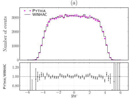
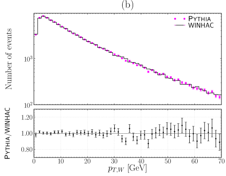
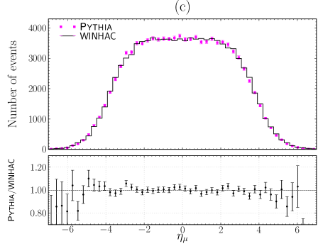
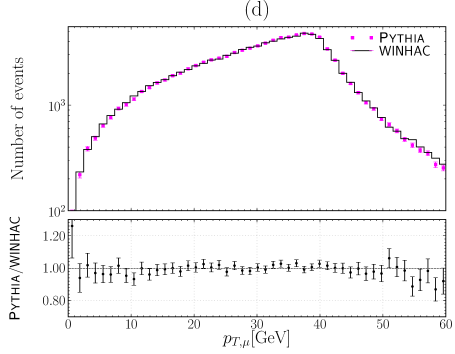
The first test, versus Pythia, is set up at the Born level with, for only higher corrections, the QCD and QED parton shower in the initial state. This imply that both data due to the structure of WINHAC are perfectly similar from both physical/technical point of view, indeed in both cases the parton shower was done by Pythia 6.403.
In Fig. 4.3 are respectively represented the rapidity and transverse momentum of the and the pseudo-rapidity and transverse momentum of the charged leptons. The validation using is important as its distribution turns out to be very sensible from the parton shower and from the intrinsic of partons (cf. Chapter 2 and Fig. 2.13.(b)). In Pythia this meant to take for these runs a Gaussian distribution for which corresponds to use the value MSTP(91)=1 with that latter corresponding to the switch PARP(91)=1. Another point, no multiple interactions were used (MSTP(81)=0). For further details on the physical and technical aspects of these parameters see Ref. [117]. As expected the data from both generator agree within the statistical limit.
For the second test WINHAC was used by adding up to the previous setting QED multi-photon radiation. On the other side to emulate higher QED radiation in Pythia the former set up was plugged to the PHOTOS [124, 125, 126] generator which added QED corrections in the final state of the events. In both cases, WINHAC and Pythia+PHOTOS, a common value was used to cut on the energies of soft photons at the level of the analysis, that is . In Fig. 4.4, the number of radiated photons are represented with the total energy of these photons. Below are represented the transverse momenta of the hardest and second hardest photons defined respectively as, for a given event, the photon with the highest and the second highest . Although the statistic is quite small for the histograms related to photons one can see there is a good agreement within the statistical error.
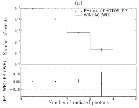
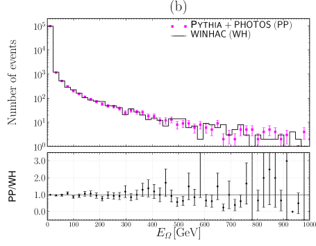
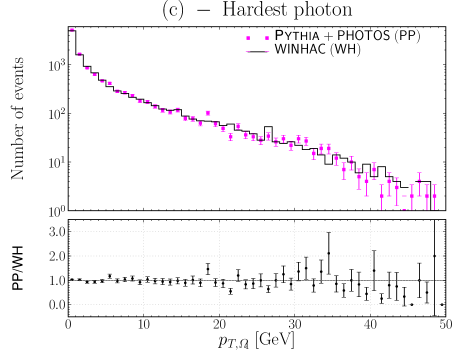
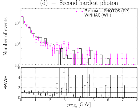
Some discrepancies were observed though while looking at the transverse mass. In Fig. 4.5 the distribution is represented for both the first validation set up and the present one. One can see in the latter case from the ratio frame that after the jacobian peak WINHAC displays a slight shift to higher with respect to Pythia(+PHOTOS). These discrepancies can be amended by the fact that here WINHAC and PHOTOS do not treat QED radiation on the same footing. Indeed, PHOTOS do not take into account cases where the one or several photon are emitted by the boson as well as the interference this creates with other diagrams where the charged lepton radiates photon(s).
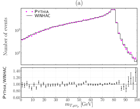
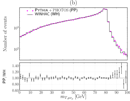
| Pythia+PHOTOS | WINHAC | |
|---|---|---|
| 0 | 88374 | 88440 |
| 1 | 10927 | 10874 |
| 2 | 677 | 664 |
| 3 | 21 | 22 |
Simulation and reconstruction tests.
The last test consisted to pass WINHAC events through the whole simulation and reconstruction chain. Tests were passed with success respectively for each time with a statistic of events using acceptance cuts of and . The low statistic is justified because of the long time it takes to simulate events. In each case the data was obtained in ESD, AOD and CBNT format.
Fig. 4.6 presents respectively comparisons between the generator and reconstructed data for the transverse momentum and pseudo-rapidity of the muon. The reconstruction was made using the MOORE algorithm [191] that reconstructs tracks in the muon spectrometer.
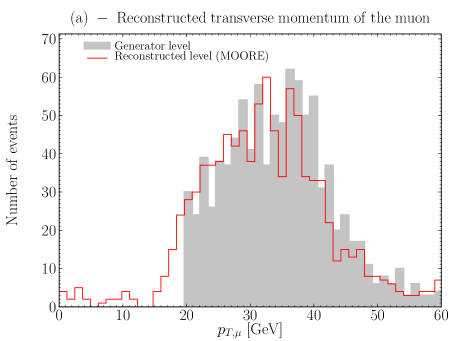
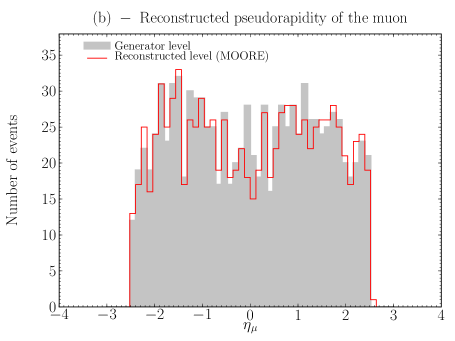
4.3 Framework of the analysis
Like explained in the introduction of this Chapter, rather than going to the refined –but heavy– framework described above a simpler and more pragmatic approach was adopted. In this approach, the simulation of the detector for the analysis is achieved using Gaussian resolution to emulate the inner detector resolution. The reason for that is that the statistic that needed to be generated is too huge to be passed through the whole simulation and reconstruction chain of the ATLAS detector. Actually, analysis with real data are based on the same principle where instead of taking the whole simulation for the detector a tuned fast simulation is used for all Monte Carlo simulation. This is for example the strategy used by CDF II for the measurement of [51].
The last argument becomes more tangible when looking quantitatively at the present analysis requirements. Studies were made for an integrated luminosity of which means an order of and . In order to optimise the strategy to measure their masses, generation and simulation of event samples was required. These samples correspond to specific biases in the detector response, or in the theoretical (phenomenological) modeling of the -boson production processes. In addition, a large number of unbiased event samples, for variable values of the masses of the and bosons, was simulated. For an assessment of the impact of the systematic biases on the overall measurement precision each of the above event sample must contains at least events in order to match the systematic and the statistical measurement precision.
The presented analysis is then based on a total sample of boson events. Generating, simulating and handling such a large event sample within reasonable limits of the storage space and computing power is challenging. Indeed, if we consider in the simplest case scenario where the gist of the event222 That is the four-momenta, types and genealogy of each particle entering in the hard process ( particles per event). would be recorded in double precision, this should require bytes for each event summaries, which leads eventually to store a Terabyte of data on disk. Besides, even though one can compute an accurate experimental simulation using GEANT, the treatment of hundreds of millions of events would be prohibitive. The computing of the desired histograms on a dedicated farm, using a fast simulation, takes 1–2 days to get all the necessary event samples.
A short descriptions of both generation and analysis framework are given below.
4.3.1 Generation framework
In that state of mind, the generation is made using the WINHAC event generator in stand-alone mode. An overview of the main features of the generation framework is represented in Fig. 4.7. For convenience the generation framework interfaced to WINHAC was also written in FORTRAN 77. This framework takes as input the physics parameters necessary for the initialisation and the running of WINHAC. During this initialisation the observables of interest are booked. Then in the generation loop, for each event, standard calling instances to WINHAC implemented by its authors allow to access basics quantities such as four-momentum, particles type, etc. from which observables of interest can be calculated. For practical reasons all analysis were made using weighted events since it is faster. At this stage, cuts or smearing to emulate the ATLAS detector resolution can be optionally applied. Eventually each observable fills the corresponding histogram and at the end of the generation the histograms are written in ASCII files along with the cross section of the process. Already at this stage histograms are normalised to according to the conventions stated in Chapter 2 § 2.3.
On our road to an experimental investigation a preliminary step consisted to look only at the generator level predictions with only optional phase-space cuts to put the spot on a particular behaviour. This is presented in the next Chapter. Then the more realistic experimental analysis for was made using some acceptance cuts related to the ATLAS performances and the smearing of the data was computed according to Eqs. (3.15–3.16) from § 3.3.2. This step us presented in Chapter 6.
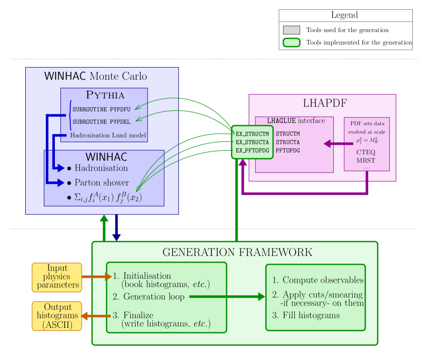
Let us note that in both cases, sometimes, changes of the original PDFs predictions needed to be done. Still, for both security and practical reasons the LHAPDF package was not touched. Instead an interface was written which lures WINHAC and Pythia to use custom values instead of the original ones. The subroutines that needed to be substituted to the use of the original ones are of the number of three and belong to the LHAGLUE interface written to mimic the old-fashion way to call PDFs from the PDFLIB package. These three subroutines which Pythia and WINHAC depend on are briefly described. The first one –the most fundamental– is STRUCTM which gives for a given PDF set at fraction and scale the parton density functions in the output form , where is such that
with, for reminder, , where (s) means sea for , and flavors. The two other subroutines, used exclusively by WINHAC, are PFTOPDG and STRUCTA and both rely on the output from STRUCTM. PFTOPDG provides the flavors in a one dimensional array which indexes, ranging from -6 to 6, are associated to the conventional ID number given to partons (see Ref. [1], Monte Carlo particle numbering scheme section). STRUCTA adds to the predictions of STRUCTM nuclear shadowing effects in the aim to compute the PDFs for a hadron of mass .
To these subroutines are substituted our custom copies
-
-
EX_STRUCTM
-
-
EX_PFTOPDG
-
-
EX_STRUCTA
the structure of the two last one are unchanged, they are just relying on EX_STRUCTM instead of the original subroutine. Then, any changes in the density functions are made by playing with the output values of EX_STRUCTM.
Let us remark that in Fig. 4.7 only the main features are given and in no case the whole chain of subroutine calling concatenation as it will eventually become obsolete as both F77 versions of WINHAC and Pythia will be replaced to C++ versions. Slight details where given for only Pythia since this Monte Carlo being extensively used its subroutines are more familiar in the high energy physics community.
4.3.2 Analysis framework
Here we describe the methods that were used to perform all kind of histograms and/or analysis from the WINHAC event generations present in this document and in our ongoing studies [72, 74]. This histograms/analysis framework is represented schematically on Fig. 4.8.
The framework is made of a central set of functions written in C++ and gathered in one *.cxx file and its associated header file *.h. This framework relies on C++ and STL (Standard Template Libraries) classes and also on ROOT classes [178, 179] from version 5.14. The ROOT classes and methods that are used essentially to handle one-dimensional double precision histograms containers TH1D and other methods inherent to this class which allow the user to perform basic operations on and between histograms. ROOT is also called to display histograms and related analysis results using the class TApp. Histograms are then displayed using the canvas class TCanvas, stored inside *.root files (using the TFile class) and postscript files for later browsing. Each step of the histograms/analysis consists always to the same principle which is to write a C++ program to reach a given goal with the help of calls of functions from our framework.
Now, further details are given on the treatment of data in a chronological order. In a first step, all the ASCII histograms obtained from the generation and sharing the same input parameters are converted to TH1D objects and stored in *.root files whose names are based on the main physical input parameters.
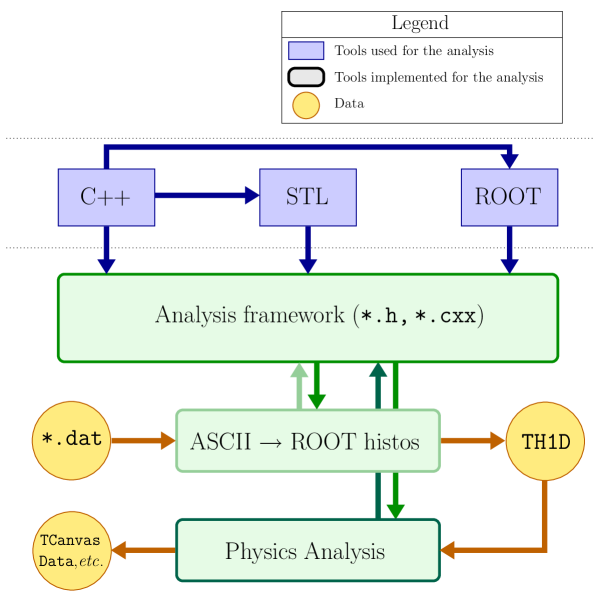
In a second intermediate step –not represented in Fig. 4.8– the newly created histograms are read from the *.root files they are stored in and displayed as TCanvas for visual cross-check. Those canvas are saved in *.root and postscript files to allow visual control for safety.
Finally the last step consists to produce the desired results that is fine histograms or an analysis. The first procedure was used extensively to understand the asymmetries in the mechanisms of production between and . For that purpose in top of drawing the two and distributions related to the observable , another frame was drawn in the canvas to display discrepancies between them. Optionally the difference, the ratio, or the charge asymmetry (Eq. (2.13)) of the two distributions was computed the latter being preferred due to the nature of the present work. This kind of analysis are presented in the next Chapter.
Concerning the physics analysis it involved to perform likelihood studies between a main () and -templates event samples distributions which template is labeled . This will be explained thoroughly in Chapter 6 here only the technical principle is described. It is very basic though, the main/templates distributions are read out from their respective *.root files and using dedicated functions of the framework a likelihood analysis is performed between each couple couple. The main histograms and all templates are displayed along with the likelihood results in canvas and saved in *.root.
Appendix 4.A Example of a WINHAC summary event
Et toi mon code pourquoi bogues tu
Comme un prompteur stroboscopique
Je scanne les nigtlies et les logsLe prompteur stroboscopique
Guillaume Apollinaire
The two columns below represent a WINHAC event displayed using a Pythia routine. This allows the reader to familiarise, if necessary, to a summary event of a high energy particle collisions from a Monte Carlo point of view. In each line are shown :
-
•
I : index of particle.
-
•
particle/jet : particle name or string (see Ref. [117] for a definition of a string in the Pythia Lund fragmentation model).
-
•
KS : gives the current status of the parton/particle. Codes from 1 to 10 correspond to currently existing partons/particles, while larger codes contain partons/particles which no longer exist, or other kinds of event information. For further details see Ref. [117], § 5.2 Event Record section.
-
•
KF : particle ID according to the convention used for the Monte Carlo numbering scheme [1].
-
•
orig : I-wise origin of the particle
-
•
p_x, p_y, p_z : Respectively the momentum components , and of the particle in the Cartesian basis attached to the laboratory inertia frame.
-
•
E, m : Energy of the particle in the Cartesian attached to the laboratory inertia frame and its invariant mass .
Event listing (summary)
I particle/jet KS KF orig p_x p_y p_z E m
1 !p+! 21 2212 0 0.000 0.000 7000.000 7000.000 0.938
2 !p+! 21 2212 0 0.000 0.000-7000.000 7000.000 0.938
==============================================================================
3 !dbar! 21 -1 1 -0.524 0.462 163.022 163.024 0.000
4 !g! 21 21 2 -0.434 -0.604 -341.373 341.374 0.000
5 !dbar! 21 -1 3 -1.249 -1.638 145.551 145.566 0.000
6 !u! 21 2 4 -2.833 -4.851 -10.211 11.654 0.000
7 !W+! 21 24 0 -4.082 -6.489 135.340 157.219 79.638
8 !mu+! 21 -13 7 -27.004 -12.899 129.225 132.645 0.106
9 !nu_mu! 21 14 7 22.922 6.410 6.115 24.575 0.000
==============================================================================
10 (W+) 11 24 7 -4.082 -6.489 135.340 157.219 79.638
11 mu+ 1 -13 8 -27.004 -12.899 129.225 132.645 0.106
12 nu_mu 1 14 9 22.922 6.410 6.115 24.575 0.000
13 n0 1 2112 1 0.612 -0.125 5009.478 5009.478 0.940
14 (ubar) A 12 -2 4 1.858 0.212 -15.901 16.014 0.330
15 (g) I 12 21 4 -0.881 0.443 0.500 1.106 0.000
16 (d) V 11 1 2 0.285 0.502-1095.905 1095.905 0.330
17 (sbar) A 12 -3 4 6.255 3.150 -145.886 146.054 0.500
18 (g) I 12 21 4 -0.621 -0.442 -9.154 9.186 0.000
19 (g) I 12 21 4 -1.436 0.954 -1.378 2.207 0.000
20 (g) I 12 21 3 0.721 2.086 15.208 15.367 0.000
21 (u) V 11 2 1 -0.088 -0.336 1827.499 1827.499 0.330
22 (s) A 12 3 4 -0.651 -0.457 -101.017 101.021 0.500
23 (g) I 12 21 4 -1.165 1.421 -36.632 36.678 0.000
24 (g) I 12 21 4 -1.146 -0.715 -18.439 18.488 0.000
25 (g) I 12 21 4 0.189 -0.306 -0.994 1.057 0.000
26 (uu_1) V 11 2203 2 0.149 0.102-5562.721 5562.721 0.771
==============================================================================
27 (string) 11 92 14 1.262 1.157-1111.306 1113.025 61.825
28 pbar- 1 -2212 27 1.512 0.037 -11.182 11.323 0.938
29 n0 1 2112 27 -0.200 0.205 -2.283 2.485 0.940
30 (pi0) 11 111 27 -0.080 -0.029 -1.056 1.068 0.135
31 pi+ 1 211 27 0.146 0.009 -1.183 1.200 0.140
32 (K*-) 11 -323 27 -0.072 0.091 -1.373 1.620 0.852
33 (Sigma*bar-) 11 -3224 27 0.007 0.183 -0.680 1.553 1.384
34 (eta) 11 221 27 -0.145 0.187 -1.360 1.485 0.547
35 (Delta++) 11 2224 27 -0.652 0.380 -26.507 26.547 1.233
36 (pi0) 11 111 27 0.501 -0.255 -7.725 7.747 0.135
37 (eta) 11 221 27 -0.640 -0.258 -43.671 43.680 0.547
38 pbar- 1 -2212 27 0.872 0.582 -50.855 50.875 0.938
39 pi- 1 -211 27 0.019 -0.425 -24.915 24.919 0.140
40 (Delta+) 11 2214 27 -0.079 -0.222 -124.802 124.808 1.287
41 (eta) 11 221 27 -0.090 -0.070 -228.547 228.548 0.547
42 (eta’) 11 331 27 0.162 0.741 -585.166 585.167 0.958
43 (string) 11 92 17 4.831 5.411 1686.290 2000.313 1075.931
44 (K0) 11 311 43 1.405 0.574 -31.106 31.147 0.498
45 pi+ 1 211 43 3.304 2.070 -95.006 95.086 0.140
46 (rho-) 11 -213 43 1.103 0.392 -20.498 20.543 0.672
47 (pi0) 11 111 43 0.057 -0.097 -0.566 0.593 0.135
48 (K*bar0) 11 -313 43 0.055 -0.031 -4.070 4.170 0.902
49 (K*+) 11 323 43 -1.041 0.270 -4.085 4.325 0.930
50 pi- 1 -211 43 0.280 0.659 -0.408 0.836 0.140
51 (omega) 11 223 43 -0.670 0.038 -0.036 1.032 0.783
52 (rho+) 11 213 43 0.102 0.550 5.466 5.530 0.623
53 pbar- 1 -2212 43 -0.106 0.362 2.722 2.904 0.938
54 p+ 1 2212 43 0.158 -0.143 6.122 6.197 0.938
55 (pi0) 11 111 43 -0.156 -0.089 3.386 3.393 0.135
56 (rho0) 11 113 43 -0.054 0.502 3.075 3.205 0.747
57 (omega) 11 223 43 0.571 -0.169 12.120 12.158 0.766
58 (pi0) 11 111 43 0.254 0.584 16.962 16.974 0.135
59 (rho0) 11 113 43 0.125 0.010 82.982 82.986 0.796
60 pbar- 1 -2212 43 -0.852 0.086 544.959 544.961 0.938
61 pi- 1 -211 43 0.370 -0.202 43.855 43.858 0.140
62 (Delta++) 11 2224 43 -0.075 0.044 1120.417 1120.417 1.172
63 (string) 11 92 22 -2.623 0.046-5719.802 5719.965 43.080
64 (Sigma*0) 11 3214 63 -0.973 0.427 -81.646 81.665 1.393
65 pi+ 1 211 63 0.002 0.040 -1.701 1.707 0.140
66 pbar- 1 -2212 63 -1.037 -0.226 -30.461 30.494 0.938
67 (K0) 11 311 63 0.026 -0.234 -25.968 25.974 0.498
68 (phi) 11 333 63 -0.227 0.399 -13.698 13.744 1.023
69 (phi) 11 333 63 -0.725 0.035 -18.106 18.149 1.019
70 (eta) 11 221 63 0.478 -0.677 -76.891 76.898 0.547
71 K- 1 -321 63 -0.332 0.361 -119.187 119.189 0.494
72 (eta’) 11 331 63 0.028 -0.076 -324.691 324.692 0.958
73 (Delta+) 11 2214 63 -0.042 -0.024-4353.561 4353.561 1.255
74 pi+ 1 211 63 0.180 0.020 -673.892 673.892 0.140
75 gamma 1 22 30 -0.016 0.026 -0.050 0.059 0.000
76 gamma 1 22 30 -0.063 -0.054 -1.005 1.009 0.000
77 K- 1 -321 32 0.144 -0.102 -0.695 0.871 0.494
78 (pi0) 11 111 32 -0.216 0.194 -0.677 0.749 0.135
79 (Lambdabar0) 11 -3122 33 -0.107 0.325 -0.576 1.301 1.116
80 pi- 1 -211 33 0.114 -0.142 -0.104 0.252 0.140
81 (pi0) 11 111 34 -0.027 -0.021 -0.422 0.444 0.135
82 (pi0) 11 111 34 -0.095 -0.013 -0.208 0.266 0.135
83 (pi0) 11 111 34 -0.023 0.221 -0.730 0.775 0.135
84 p+ 1 2212 35 -0.728 0.292 -24.709 24.740 0.938
85 pi+ 1 211 35 0.076 0.088 -1.798 1.807 0.140
86 gamma 1 22 36 0.014 -0.035 -0.288 0.290 0.000
87 gamma 1 22 36 0.487 -0.220 -7.437 7.457 0.000
88 (pi0) 11 111 37 -0.072 0.017 -4.828 4.830 0.135
89 (pi0) 11 111 37 -0.226 -0.159 -13.516 13.520 0.135
90 (pi0) 11 111 37 -0.342 -0.117 -25.327 25.330 0.135
91 p+ 1 2212 40 -0.286 -0.151 -111.230 111.235 0.938
92 (pi0) 11 111 40 0.207 -0.071 -13.571 13.574 0.135
93 (pi0) 11 111 41 -0.113 -0.013 -43.560 43.560 0.135
94 (pi0) 11 111 41 -0.082 0.017 -94.359 94.359 0.135
95 (pi0) 11 111 41 0.105 -0.074 -90.628 90.629 0.135
96 pi+ 1 211 42 -0.059 0.227 -99.601 99.602 0.140
97 pi- 1 -211 42 0.179 0.111 -118.078 118.078 0.140
98 (eta) 11 221 42 0.043 0.403 -367.487 367.488 0.547
99 K_L0 1 130 44 1.405 0.574 -31.106 31.147 0.498
100 pi- 1 -211 46 0.893 0.545 -15.636 15.672 0.140
101 (pi0) 11 111 46 0.210 -0.153 -4.862 4.871 0.135
102 gamma 1 22 47 -0.016 0.018 -0.027 0.037 0.000
103 gamma 1 22 47 0.074 -0.115 -0.539 0.556 0.000
104 (Kbar0) 11 -311 48 -0.240 -0.103 -2.248 2.317 0.498
105 (pi0) 11 111 48 0.295 0.072 -1.823 1.853 0.135
106 K+ 1 321 49 -0.294 0.117 -1.161 1.301 0.494
107 (pi0) 11 111 49 -0.747 0.153 -2.924 3.025 0.135
108 pi- 1 -211 51 -0.155 -0.163 -0.109 0.286 0.140
109 pi+ 1 211 51 -0.448 -0.020 0.006 0.470 0.140
110 (pi0) 11 111 51 -0.067 0.220 0.067 0.275 0.135
111 pi+ 1 211 52 -0.135 -0.024 1.032 1.050 0.140
112 (pi0) 11 111 52 0.237 0.574 4.434 4.479 0.135
113 gamma 1 22 55 -0.166 -0.084 3.357 3.362 0.000
114 gamma 1 22 55 0.010 -0.005 0.028 0.031 0.000
115 pi+ 1 211 56 -0.192 0.081 2.198 2.212 0.140
116 pi- 1 -211 56 0.137 0.421 0.878 0.993 0.140
117 pi+ 1 211 57 -0.085 -0.066 1.508 1.519 0.140
118 pi- 1 -211 57 0.333 0.078 6.207 6.218 0.140
119 (pi0) 11 111 57 0.323 -0.181 4.405 4.422 0.135
120 gamma 1 22 58 0.046 0.033 2.242 2.243 0.000
121 gamma 1 22 58 0.208 0.551 14.720 14.732 0.000
122 pi+ 1 211 59 -0.118 -0.322 36.308 36.310 0.140
123 pi- 1 -211 59 0.243 0.333 46.674 46.676 0.140
124 p+ 1 2212 62 0.085 0.068 828.515 828.516 0.938
125 pi+ 1 211 62 -0.160 -0.023 291.902 291.902 0.140
126 (Lambda0) 11 3122 64 -0.739 0.123 -61.419 61.434 1.116
127 (pi0) 11 111 64 -0.234 0.304 -20.227 20.231 0.135
128 (K_S0) 11 310 67 0.026 -0.234 -25.968 25.974 0.498
129 K_L0 1 130 68 -0.116 0.221 -8.379 8.397 0.498
130 (K_S0) 11 310 68 -0.111 0.178 -5.319 5.346 0.498
131 K- 1 -321 69 -0.226 -0.026 -7.284 7.305 0.494
132 K+ 1 321 69 -0.500 0.061 -10.821 10.844 0.494
133 (pi0) 11 111 70 0.080 -0.021 -16.763 16.764 0.135
134 (pi0) 11 111 70 0.127 -0.169 -19.715 19.717 0.135
135 (pi0) 11 111 70 0.270 -0.488 -40.412 40.417 0.135
136 pi+ 1 211 72 0.058 -0.015 -25.415 25.416 0.140
137 pi- 1 -211 72 0.046 0.109 -69.547 69.547 0.140
138 (eta) 11 221 72 -0.077 -0.169 -229.728 229.729 0.547
139 p+ 1 2212 73 0.154 0.148-3338.310 3338.310 0.938
140 (pi0) 11 111 73 -0.197 -0.171-1015.251 1015.251 0.135
141 gamma 1 22 78 -0.045 0.117 -0.198 0.235 0.000
142 gamma 1 22 78 -0.171 0.076 -0.479 0.514 0.000
143 nbar0 1 -2112 79 -0.145 0.351 -0.561 1.158 0.940
144 (pi0) 11 111 79 0.038 -0.026 -0.015 0.143 0.135
145 gamma 1 22 81 -0.025 -0.060 -0.386 0.392 0.000
146 gamma 1 22 81 -0.002 0.039 -0.035 0.052 0.000
147 gamma 1 22 82 -0.054 -0.071 -0.145 0.170 0.000
148 gamma 1 22 82 -0.041 0.059 -0.063 0.096 0.000
149 gamma 1 22 83 -0.069 0.149 -0.368 0.403 0.000
150 gamma 1 22 83 0.046 0.072 -0.362 0.372 0.000
151 gamma 1 22 88 0.003 0.064 -2.343 2.344 0.000
152 gamma 1 22 88 -0.075 -0.047 -2.485 2.486 0.000
153 gamma 1 22 89 -0.100 -0.104 -9.627 9.628 0.000
154 gamma 1 22 89 -0.125 -0.055 -3.889 3.892 0.000
155 gamma 1 22 90 -0.035 -0.055 -2.797 2.798 0.000
156 gamma 1 22 90 -0.307 -0.061 -22.530 22.532 0.000
157 gamma 1 22 92 0.145 -0.059 -12.182 12.183 0.000
158 gamma 1 22 92 0.062 -0.012 -1.390 1.391 0.000
159 gamma 1 22 93 0.008 -0.042 -5.984 5.985 0.000
160 gamma 1 22 93 -0.121 0.029 -37.575 37.576 0.000
161 gamma 1 22 94 -0.117 0.030 -75.044 75.044 0.000
162 gamma 1 22 94 0.035 -0.013 -19.315 19.315 0.000
163 gamma 1 22 95 0.007 -0.034 -4.705 4.705 0.000
164 gamma 1 22 95 0.098 -0.040 -85.923 85.923 0.000
165 gamma 1 22 98 -0.038 0.501 -336.480 336.481 0.000
166 gamma 1 22 98 0.080 -0.097 -31.007 31.007 0.000
167 gamma 1 22 101 0.022 -0.008 -1.605 1.605 0.000
168 gamma 1 22 101 0.187 -0.145 -3.257 3.266 0.000
169 K_L0 1 130 104 -0.240 -0.103 -2.248 2.317 0.498
170 gamma 1 22 105 -0.001 0.023 -0.292 0.293 0.000
171 gamma 1 22 105 0.296 0.049 -1.531 1.560 0.000
172 gamma 1 22 107 -0.045 0.045 -0.209 0.218 0.000
173 gamma 1 22 107 -0.702 0.109 -2.715 2.806 0.000
174 gamma 1 22 110 -0.019 -0.015 -0.006 0.025 0.000
175 gamma 1 22 110 -0.048 0.235 0.073 0.251 0.000
176 gamma 1 22 112 0.088 0.092 1.106 1.113 0.000
177 gamma 1 22 112 0.149 0.482 3.328 3.366 0.000
178 gamma 1 22 119 0.278 -0.171 4.193 4.205 0.000
179 gamma 1 22 119 0.045 -0.009 0.212 0.217 0.000
180 n0 1 2112 126 -0.554 0.177 -48.857 48.870 0.940
181 (pi0) 11 111 126 -0.185 -0.054 -12.562 12.564 0.135
182 gamma 1 22 127 -0.081 0.191 -8.389 8.392 0.000
183 gamma 1 22 127 -0.153 0.114 -11.838 11.839 0.000
184 (pi0) 11 111 128 -0.086 0.005 -3.284 3.288 0.135
185 (pi0) 11 111 128 0.112 -0.239 -22.684 22.686 0.135
186 (pi0) 11 111 130 0.149 0.008 -1.913 1.923 0.135
187 (pi0) 11 111 130 -0.260 0.171 -3.406 3.423 0.135
188 gamma 1 22 133 0.049 -0.066 -5.428 5.429 0.000
189 gamma 1 22 133 0.031 0.045 -11.335 11.335 0.000
190 gamma 1 22 134 0.118 -0.192 -17.526 17.528 0.000
191 gamma 1 22 134 0.009 0.023 -2.189 2.189 0.000
192 gamma 1 22 135 0.137 -0.370 -29.014 29.017 0.000
193 gamma 1 22 135 0.134 -0.118 -11.398 11.400 0.000
194 gamma 1 22 138 0.000 -0.042 -214.479 214.479 0.000
195 gamma 1 22 138 -0.077 -0.127 -15.250 15.250 0.000
196 gamma 1 22 140 -0.142 -0.183 -725.604 725.604 0.000
197 gamma 1 22 140 -0.054 0.012 -289.647 289.647 0.000
198 gamma 1 22 144 0.079 0.006 -0.036 0.087 0.000
199 gamma 1 22 144 -0.042 -0.032 0.021 0.056 0.000
200 gamma 1 22 181 -0.137 0.004 -10.352 10.353 0.000
201 gamma 1 22 181 -0.048 -0.059 -2.211 2.212 0.000
202 gamma 1 22 184 -0.004 -0.046 -1.886 1.887 0.000
203 gamma 1 22 184 -0.082 0.051 -1.397 1.401 0.000
204 gamma 1 22 185 0.019 0.010 -0.734 0.734 0.000
205 gamma 1 22 185 0.092 -0.249 -21.950 21.952 0.000
206 gamma 1 22 186 0.078 0.070 -1.148 1.153 0.000
207 gamma 1 22 186 0.071 -0.062 -0.765 0.771 0.000
208 gamma 1 22 187 -0.067 0.060 -1.702 1.705 0.000
209 gamma 1 22 187 -0.193 0.111 -1.704 1.718 0.000
sum: 2.00 0.00 0.00 0.00 14000.00 14000.00
Chapter 5 Phenomenology of and in Drell–Yan like processes at the LHC
Super Skrull Warrior : “I have trained my entire life to face you.”
Black Panther : “Then you have already lost. For I have trained my entire life to face the unknown.”Black Panther #39 - See Wakanda and Die (September 2008)
This Chapter presents the phenomenology of the and bosons production in Drell–Yan processes at the LHC. This preliminary work is mandatory before addressing any kind of study related to the extraction of the boson properties. Indeed, the LHC in top of supplying unprecedented luminosity and energy in collisions will provide –due to the nature of the colliding beams– original kinematics with respect to the one inherent to collisions studied exhaustively for these last decades at the SPS and Tevatron colliders. These original LHC features demand to start with basics understanding before addressing a more complete analysis prospect.
The Chapter is divided as follow. In a short introduction the context of the studies is described from both physics and technical point of view. Then comes the phenomenological understanding of the and bosons production in Drell–Yan, first by looking at the production of and then at the whole process by studying the properties of the decaying charged leptons.
Let us stress that before reaching the refined understanding presented here more thorough analysis were done using complementary distributions, different physical input parameters, for specific domains of the phase-space, etc. Nonetheless, to keep the discussion as clear as possible in the core of the Chapter all these exhaustive studies are compiled in Appendix 5.A.
5.1 Context of these studies
The most relevant kinematics to the in Drell–Yan are reviewed at the generator level, that is looking only at the purely phenomenological level.
Among all the observables/pseudo-observables that entered in our study only a few were kept in the core of the Chapter. They are of two categories. First are the pseudo-observables characterising the boson properties, its rapidity and transverse momentum . Then are the observables characterising the charged lepton properties, its pseudo-rapidity and transverse momentum that allows to study the whole process. The definitions of these quantities and the information they hold for in Drell–Yan have been over-viewed in Chapter 2 § 2.4.2.(d) for the case of a charge blind study. Here, based on this previous overview a fine study of the positive and negative channel is considered.
The type of collisions considered are : , and . The collision scheme is considered as a reference since in that case the production of and are on the same footing and the characteristics of the kinematics are well known from the experience gathered from SPS and Tevatron colliders. Standard LHC collisions are analysed as well with isoscalar beams collisions on the example of deuteron–deuteron () targets which is justified for both pedagogical means and because the strategy prospect in the next Chapter relies on such a scheme. The nucleon–nucleon center of mass energy is of for and collisions and of for collisions according to the expected LHC capabilities (cf. Eqs. (3.11–3.12)). The choice of in the center of mass energy for is justified by the wish to put the energy scales and accessible phase space to the particles on the same footing as the one for collisions to stress the differences between these two collision schemes. The total hadronic cross sections corresponding to these collisions and computed by WINHAC are gathered in Table 5.1.
| Collider | [nb] | [nb] | [nb] |
|---|---|---|---|
Now details are given on the material presented below from a more technical point of view. All the histograms were produced using the WINHAC Monte Carlo event generator at the truth level within improved leading order defined from the physics point of view in Chapter 2 § 2.4.2.(d) and from a Monte Carlo point of view in Chapter 4 § 4.1.2. A common statistic of millions weighted events were used for each and channel and for all type of collisions. The decay of the bosons was opened to both electronic and muonic channels. Every histograms were generated with 200 bins and for visual convenience this former binning was reduced later on at the analysis level when necessarily. The remaining input parameters of importance for the generation are :
Let us remind the conventions used for the coordinate systems and the definitions of the common kinematics are gathered in Chapter 2 § 2.3. In this context, collisions are defined in the Cartesian basis, with the proton moving in the direction while the anti-proton moves in the direction. In what follows the discrepancies between the positive and negative channels predictions are scrutinised using the charge asymmetry (Eq. (2.13)).
5.2 Production of and bosons
In this Section the boson production mechanism is discussed via the analysis of the boson rapidity and transverse momentum . Figure 5.1 presents the latter distributions for and bosons, as well as their associated charge asymmetries in and collisions.
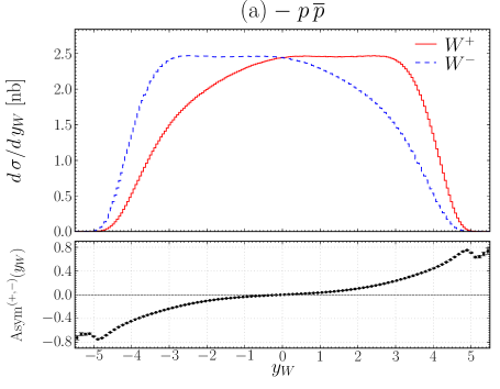
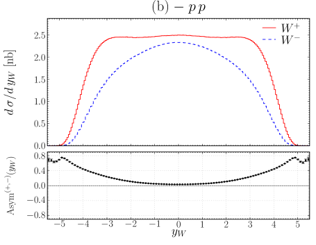
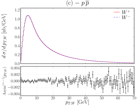
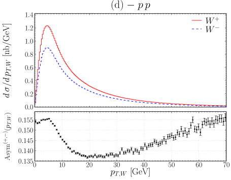
Our observation starts with the well known kinematics. Let us remind the and bosons are produced with the same dynamics due to the nature of the colliding beams. Indeed, the same amount of matter and antimatter are available to produce a or a . The most visible difference between the two processes occurs at the spatial level because the proton and anti-protons are always impinging respectively from the and directions. Thus the kinematics between the and event samples differ only from a mirror reflection with respect to the plane passing by the origin. More explicitly, to each phase space configuration of amplitude of probability for the boson corresponds another phase space configuration for the in which and that has the exact same amplitude. The evidence for this behaviour can be seen already for the bosons longitudinal component when looking at the rapidity (Fig. 5.1.(a)) where one can see the and distributions are the same up to a vertical flip with respect to the origin. Concerning the and transverse momenta the symmetry is such that it makes no differences between the two channels when projecting on the plane as shown in Fig. 5.1.(c). From the point of view of a extraction the important thing is that distributions are independent of the boson charge which means the leptons, as it will be confirmed, undergo the same boosts.
Now Figures 5.1.(b) and (d) show the corresponding distributions for collisions. Here both rapidity distributions are symmetric with respect to which is the consequence of the identical nature of the colliding targets. The shapes of the spectra are different for the and bosons which reflects the difference in the valence and quark content and properties in a proton. The distribution for the boson is higher and wider with respect to the one for the boson. First let us note there are twice as many valence quarks as valence quarks explaining the higher differential cross section for . Besides, quarks carry, in average, a higher fraction of the parent proton momentum (cf. Fig. 2.11), which, assuming respects to a good approximation the LO expression of Eq. (2.82), implies that are more likely to have a higher absolute values rapidity. This explains the wider behaviour of compared to .
The charge asymmetry in the distribution reflects both the differences in the relative cross sections but also, what will be crucial for the studies presented in this Chapter, in the shape of their distributions. The nontrivial shape of is due to the flavour asymmetries in the distributions of quarks producing and bosons. The latter are predominantly driven by the – quark asymmetries. Then the CKM mixing involves the other , and flavours among which –as it will be shown– the non equality of the and quark masses add up to the main – charge asymmetries. This can be analysed with the flavour structure of the bosons charge asymmetries by writing explicitly the simplified Born level formulæof the total cross section charge asymmetries for and collisions
| (5.1) | |||||
| (5.2) | |||||
where in these expressions and on the right hand side denote the PDFs of the corresponding quark flavours and the superscript stands for valence quarks, is the CKM matrix element for the and flavours, while is the “CKM matrix element stripped” partonic cross section for the boson production with . Let us stress that the above expressions are over simplified for pedagogical reasons and do not reflect the physics implemented in the WINHAC event generation. We have omitted the explicit dependence of the PDFs on the factorisation scheme, on the transverse momenta of annihilating partons present both in the “-non integrated” PDFs, and in the partonic cross sections (via dependence of ). All the above effects are present in WINHAC. In our analysis partons have both the primordial transverse momenta and the perturbative generated ones as modeled by the initial state parton shower of the Pythia generator. Their transverse momenta depend on the Bjorken of the annihilating (anti-)quark and, for heavy quarks (here and ), also on their masses (see Ref. [117] for more details).
As one can see in Eq. (5.1), the charge asymmetry disappears for the collision mode if, as assumed in the presented studies . Let us note that this equality holds no matter the level of the corrections embraced in the calculus. Therefore, this collision scheme would be, on a theoretical level, the optimal one for measuring . Any deviation from the equality of the masses would result in non zero asymmetries regardless of the level of understanding of the flavour and momentum structure of the beam particles. For collisions several effects, reflecting the present understanding of the partonic content of the beam particles –in particular, the understanding of the momentum distribution of valence quarks– contribute to the charge asymmetry of the distribution and may mimic effects.
The asymmetries in collisions can be really reduced when going to isoscalar collisions. For example in collisions the asymmetries in the quark flavour can be deduced easily from Eq. (5.2) by considering here . We obtain then
| (5.3) |
where here the PDFs have to be understood as the parton distributions functions inside a deuteron contrary to Eqs. (5.1–5.2) where they were the one related to the proton. This was omitted on purpose not to overload the expressions. Here then, the asymmetry is driven by the Cabibbo suppressed difference of the distribution of the strange and charm quarks, weighted by the distributions of the valence quarks. The collision scheme is introduced at this point in order to analyse the relative importance of the valence quark and “” effects.
In what follows the numerical importance of the various terms appearing in the above equations is studied. For that purpose, to visualise the size coming from certain quarks contributions we reject all the contributions which we are not interested in (basically weight these events by zero) and in some occasions we modify the predictions of the PDFs by hand using the framework described in Fig. 4.7 of § 4.3.1. The results are presented in Fig. 5.2 by looking each time at .
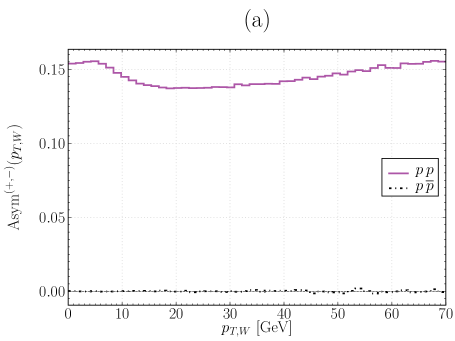
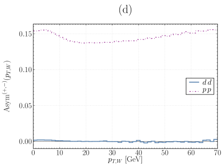
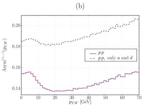
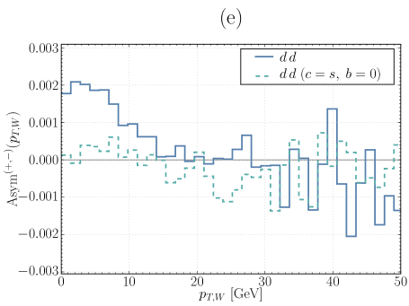
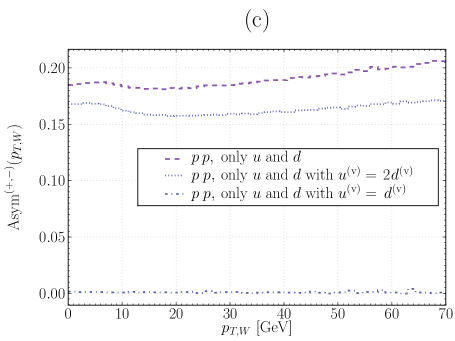
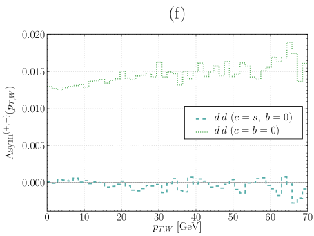
The first frame (a) compares collisions with the charge asymmetry free collisions. The charge asymmetry for collisions is large and is varying with .
The next frame, (b), shows the comparison of the asymmetry from the previous plot with the case where only the “” contributions ( for production and for production) have been kept. The small gap between the two curves, compared to the size of the latter, reflects the small overall influence of , and flavours in the asymmetry compared to the contribution of the and quarks.
Frame (c) demonstrates this asymmetry is slightly reduced when in top of having only and quarks we have , i.e. when the and valence quark PDFs are assumed to have the same shape and differ only by the normalisation factor corresponding to their number in the proton. In addition, let us note that the asymmetry becomes flatter as a function of indicating the role of the relative -shape of the and quarks PDFs. Finally, the asymmetry is reduced drastically when adding to the previous constraints , as it would be the case when colliding isoscalar beams. This shows the consequences of for , which was found to be of the order of . In the rest of the plots the simplest isoscalar beam collision scheme, , is considered.
The frame (d) shows that the charge asymmetry for is much smaller than the one for with only small discrepancies mainly at low . This results from the two following facts : (1) now all the terms contributing to the charge asymmetry include only off-diagonal CKM matrix elements and (2) contributions of the , and quark PDFs are smaller than the ones coming from sea and quark PDFs. Hence this shows how in collisions the bulk of the charge asymmetries comes from the term in Eq. (5.2).
The remaining charge asymmetry is at the level of as can be seen in the zoomed frame (e) and it can be reduced to a statistically negligible level when setting and rejecting quarks contributions. The first constraint, because , assures to cancel the two first terms in the bracket of the RHS of Eq. (5.3) while the second finalise the rise of any asymmetry.
Finally the frame (f) shows the effect of the deviation of the charge asymmetry due to the difference of the masses and of the momentum distributions of the strange and charm quarks in the extreme case where the contributions are rejected as well with the collisions involving . In that case, the obtained asymmetry is significantly higher, at a level of . It is a factor of bigger than the asymmetry for the collisions assuming the present understanding of the relative asymmetry in the distribution of the strange and charm quarks.
In the analysis presented so far the distribution is inclusive, in other words it has been integrated over the full range of allowed and . In order to optimise the measurement strategy of the mass charge asymmetry, we now discuss the charge asymmetry distributions restricted to selected kinematics regions. The most obvious method to reduce the contributions of the valence quarks is to restrict the analysis to the region, where , i.e. where the valence quarks are largely outnumbered by the sea quarks.
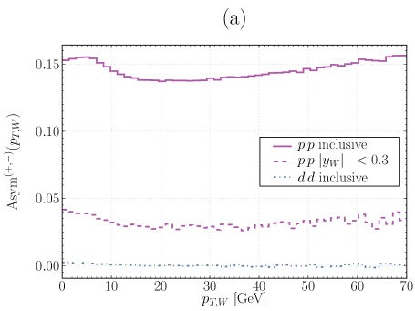
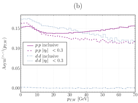
Figure 5.3 presents the asymmetries for and collisions for the narrow central bins in the rapidity (a), and in the lepton pseudo-rapidity (b). In the frame (a) the charge asymmetry is reduced and flattened by more than a factor of for the range of the boson rapidity . Now since cannot be measured directly it is natural to check if a comparable reduction can be obtained using the variable which is correlated with . Unfortunately, this is not the case, as shown in frame (b). The variable has thus significantly lower discriminative power to reduce the valence quark contribution with respect to the variable. For the collisions the asymmetry restricted to the narrow bin increases considerably. This observation draws our attention to the fact that the asymmetry in the decay mechanism of the and bosons will have an important impact on the asymmetry of leptonic observables. This will be discussed in detail in the next section.
Let us conclude by noticing there can also be a contribution to the charge asymmetry coming from the QED radiation from quarks, as upper and lower components of quark doublets have different electric charges. However, it was found with the Pythia parton shower model to be of the order of , which is insignificant compared to the other previous contributions to the asymmetries for and .
5.3 Decays of and bosons
In this section the boson decay mechanism and its influence on the charge asymmetries are studied in both and collisions by looking at the charged lepton pseudo-rapidity and transverse momentum spectra.
First, in an overview, we see why in collisions we continue to observe perfectly symmetric features while in collisions we observe larger charge asymmetries than in the initial state due to the decay properties of the leptons. After that, to emphasise the arguments delivered in the previous overview a detailed description of the and decays in specific regions of -space is presented.
5.3.1 Overview in proton–anti-proton and proton–proton collisions
Figure 5.4 presents the charged lepton and distributions along with their associated charge asymmetries. Let us start by noticing that when studying the pattern of the spectra the influence of can be neglected in the discussion since . More qualitatively, the improved LO affects the LO differential cross sections only to maximum, thus –just in those cases– we can consider .
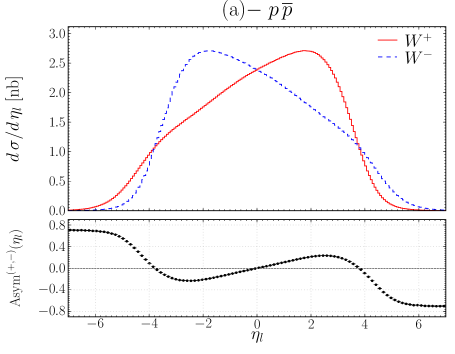
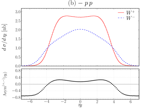
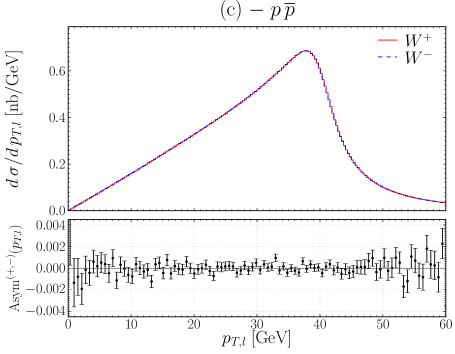
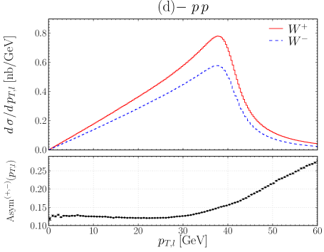
Proton–anti-proton collisions.
Starting with collisions one can see the distributions (Fig. 5.4.(a)) are each other mirror reflection with respect to this being a consequence of the symmetry of the problem as discussed in the previous section. Here it simply translates into that the whole event generation is exactly the same than the one of the up to the transformation .
Once again this symmetry implies that projecting the charged leptons momenta on the plane gives identical distributions for positive and negative charges which is shown in Fig. 5.4.(c).
Proton–proton collisions.
For collisions, on the other hand, at first sight the positively and negatively charged leptons display highly non symmetric behaviour between each other. The pseudo-rapidity distributions indicates that leptons decay preferentially in the opposite direction of while leptons display the inverse behaviour (Fig. 5.4.(b)). The size of the charge asymmetry in is much larger than the one in and further investigations proved it is explained by the privileged decay of leptons in the direction of while leptons decay in most cases in the opposite direction of (Fig. 5.4.(d)). The reason for these two behaviours in and finds its fundamental origin in the coupling of the leptons to the bosons. Indeed, as seen in Chapter 2, at the level of the differential partonic cross section the angular distribution in the RF of the final state charged lepton decaying from a boson of a given polarisation state can be expressed
| (5.4) | |||||
| (5.5) |
where, for reminders, is the charged lepton polar angle with respect to the direction of the momentum in the laboratory frame (Eq. (2.44)), is the boson electric charge in units of and is the boson helicity. As can be seen, the angular distributions of and for longitudinally polarised bosons ( for ) are the same while for the transversely polarised bosons ( for ), they depend upon the boson helicity. To simplify the rest of the argumentation we will not consider the decay of longitudinally polarised . This leaves us with transversely polarised bosons which, due to the excess of matter from valence quarks111From another point of view the charge asymmetries can be seen as the consequence of a lack of anti-matter (valence anti-quarks) that cannot match this excess of matter from valence quarks. in LHC collisions, are produced in larger proportions with negative helicities, i.e. .
The consequences of this excess of accounts for the behaviour of the pseudo-rapidity distributions illustrated in Fig. 5.5 in both RF and laboratory frame (LAB) : access larger pseudo-rapidity than the . Note this behaviour is already observed at leading order where and is only slightly affected by in the improved LO. The features observed in the longitudinal direction being understood we now turn our attention to the asymmetric pattern present in the transverse direction.

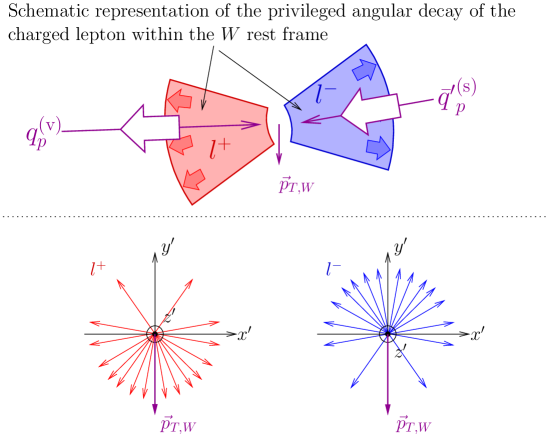
As explained above a deeper investigation shows the leptons decay preferentially in the direction of while the lepton display the inverse behaviour. This effect is the result of the coupling properties folded to the transverse motion of the or, more precisely, the relative size of the valence and sea (anti-)quarks in the collision. Indeed, in a collision involving a valence quark the sea anti-quark carries in general a higher transverse motion (cf. § 5.A.6) which, as can be understood using kinematic momentum conservation rules of thumb, constrains the charged lepton to privilege a certain azimuthal direction depending on the helicity it is holding. Figure 5.6 illustrates these effects, since the leptons have a positive helicity, aligning it on the one of the sea quarks constrains it to decay in the same direction of the anti-quark and by extension, since the latter carries most of the transverse motion, with the one of . On the other hand negative helicity leptons, under the same kinematics, are constrained to prefer a decay in the opposite direction of the anti-quark/. Eventually it turns out the leptons intrinsic transverse momentum are amplified by while in the case of the leptons they are reduced by . Let us emphasise that even though this effect is ignited by the coupling attribute its amplitude depends of the relative unbalance in the transverse motion of the colliding valence quark and sea anti-quark, which is governed by the colliding energy in the center of mass. Also worth noticing is that even at the leading order there are already charge asymmetries in the spectra, still, due to their smaller size with respect to the one discussed above, their study is treated in § 5.A.4.
In the rest of this section the previous distributions are reviewed for two narrow absolute rapidity regions, respectively in a central domain () and in a forward domain (). In the central region, the bosons are produced from quark–anti-quark pairs having leading to small valence quarks contributions, and as a consequence, the assumed isospin symmetry in sea quarks flavours cannot produce charge asymmetries. On the other hand, in the forward region the production of bosons involve most of the time a a valence (anti-)quark in collisions and a valence quark in collisions.
5.3.2 Proton–anti-protons collisions
The explanations in this subsection can be followed looking at Fig. 5.7 showing the , and distributions in and rapidity regions.
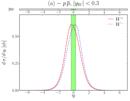
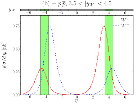
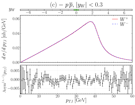
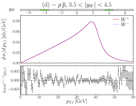
and pseudo-rapidity distributions.
In the narrow central rapidity region as it has been established valence (anti-)quark contributions are rather small, then and leptons display in a first approximation the same behaviour. The discrepancies come from the small influence of valence (anti-)quarks.
In the forward rapidity region the valence (anti-)quarks influence creates large local asymmetries in both and distributions. Those behaviours can be understood looking at the pseudo-rapidity. Using the LO approximation from Eq. (2.92) gives
| (5.6) | |||||
| (5.7) |
where and are respectively the intrinsic rapidity of the positively and negatively charged leptons. The rapidity of the is much larger than the intrinsic (cf. § 2.4.2), also the pattern of the distributions in Fig. 5.7.(b) can be seen as the consequence of : (1) the high longitudinal component of the boost that fixes roughly the center of the spectrum at and (2) the polar decay of the lepton –ruled by the coupling– which smears the distribution from the central “-induced” value. Let us look at the case of the lepton . In the region , bosons are produced mainly via pair collision, where for reminder stands for valence and for sea. In other words we have mostly which, combined to the coupling constrain the decaying to be preferentially emitted in the opposite direction to . This can be seen as most of the distribution tends to shift to lower values of . On the other side, where , bosons are produced mainly via annihilation which gives . Here the decaying lepton prefers to be emitted following the direction. Let us note the difference of height between two opposite bumps comes from the fact that . The same ideas can be applied to the case of the lepton decay, this time the opposite behaviour is observed with the exact same proportions
and transverse momenta distributions.
The forward rapidity region is exclusively addressed as we know the issues related to the valence contributions are more important there. In the RF, the spectrum of the relative angle between the and the in is exactly the same than the one between the and the in as shown in Fig. 5.7.(b). This is true independently of the relative unbalance in the colliding quark–anti-quark , thus the boost are identical and give eventually the same kinematics –up to a vertical flip– for the and from these opposite -space domains. The same idea can be used to account for the equality of the distribution in with the distribution in . Then, as long the rapidity selection is achieved on the absolute value the positive and negative leptons transverse momenta show no asymmetries as displayed in Fig. 5.7.(d). This property is obviously conserved when integrating over the whole phase space.
5.3.3 Proton–proton collisions
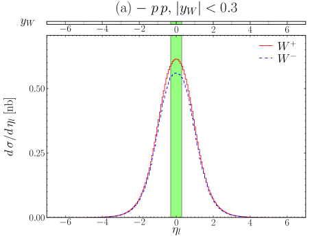
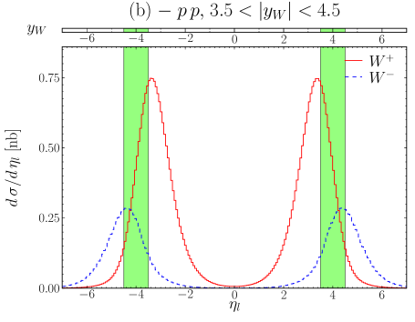
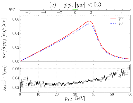
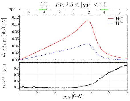
Considering now the case of collisions we repeat the same path of reasoning followed for the case. The and distributions in collisions for the narrow central and forward rapidity regions are shown in Fig. 5.8.
Pseudo-rapidity distributions.
Once again going to allows to get rid of most of the valence quarks which, as it was found out in the overview is the source of the asymmetries in collisions (Fig. 5.8.(a)). The small discrepancies are due to non negligible contributions from valence quarks.
Now moving to the region (Fig. 5.8.(b)) the general pattern can be understood using Eqs. (5.6–5.7). Both and distributions are found in the vicinity of and the deviations from this central value are due to lepton decay in ruled by the coupling, i.e. only positive helicity and negative helicity can couple to bosons.
We start by analysing the positively charge lepton . Here, in both positive () and negative () rapidity domains the are produced most likely from a annihilation providing to the boson a negative helicity. Then the preferentially decay in the opposite direction of . This explains why the spectrum is slightly shifted to smaller absolute values. The same idea can be applied to the other charged lepton. One finds eventually that this time the decays in most cases in the same direction of which translates here that the spectrum is slightly shifted to higher absolute values of . This explains why we observed in Fig. 5.4.(b) a widening of the pseudo-rapidity distribution from while the pseudo-rapidity tends to narrow from the inner spectrum. The relative size of the peaks is explained to the light that, as said previously, in a proton there are more than .
Let us stress that the differences between the -bands width and the associated spread distributions demonstrates that has a significantly weaker resolution power for the momenta of annihilating quarks than , and, as a consequence, weaker resolving power of the boson polarisation. This gives already an idea of the loss of information one has to accept when trading the knowledge of the rapidity with the charged lepton pseudo-rapidity.
Transverse momenta distributions in forward rapidity region.
The behaviour of the charged lepton transverse momenta are discussed exclusively in the forward rapidity region (Fig. 5.8.(d)). For , in the RF the relative angle between the and the is different from the one of and the due to the larger value of the sea quark transverse momentum with respect to the one of the valence quark. The coupling as shown in Fig. 5.6, by forcing the and to decay in opposite direction induce the to follow the transverse motion held mostly by the sea quark while the decays in the opposite direction of the latter. Taking into consideration the negative rapidity stripe concurs to roughly double the size of the asymmetry. The consequences of this effect on the pattern of the transverse momenta of the and has dramatic effects.
Figure 5.9 quantifies this important aspect at the inclusive level by displaying the spectra which is defined as the azimuthal angle of the charged lepton in the RF with respect to the direction of the transverse momentum of the boson in the laboratory frame, that is
| (5.8) |
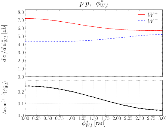
In conclusion the absence of valence anti-quarks makes the production of and at the LHC irretrievably different. The increase of the transverse momenta of the bosons produced at high absolute rapidity amplifies the impact of the boson polarisation asymmetry on the charge asymmetry of its decay products. These effects will give rise to important measurement biases which were not present in the collision mode but will show up in the measurement of the boson properties in the LHC collision mode.
In order to illustrate a little bit more the charge asymmetry in Figure 5.10.(a) shows the imperfect match between the and histograms when normalised to unit. This demonstrates that the difference of scale being removed the discrepancies are important enough to be noticed by the eye. Especially frame (b) shows a zoom on the jacobian peak which shape is of crucial importance for the extraction of the boson mass. In particular we can distinguish a particular feature, that is at the LHC energies we are to expect :
| (5.9) |
where is the average of the charged lepton . To be more precise, using the WINHAC Monte Carlo event generator for a statistic of inclusive events we find
| (5.10) | |||||
| (5.11) |
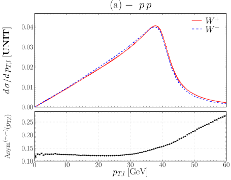
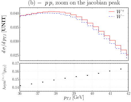
5.3.4 More details on the leptons transverse momenta charge asymmetry in collisions
To analyse a little bit more the relative position of the jacobian peaks between the two channels, distributions were studied for narrow central and forward and , respectively and selections as shown in Fig. 5.11. The selection in being justified to show how the ambiguity becomes large when making a selection with the latter. This gives complements on the low -selection resolution one have to deal when relying on rather than .
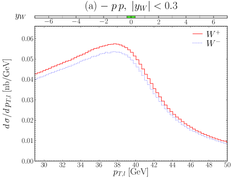
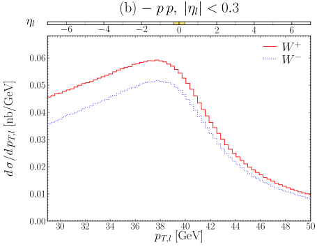
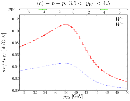
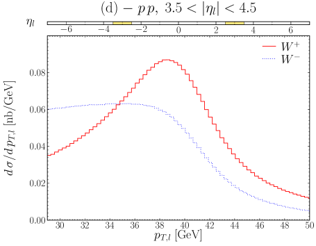
To quantify the impact on the jacobian peak position we applied an empirical procedure consisting into fitting and spectra by a polynomial of second order in the vicinity of the peak. This range was taken to be . The value corresponding to the two parabolas are noted for and for the one of . The difference between these two position is considered to quantify the variation of the peaks position. The results are gathered in the table below
| phase space domain | [MeV] |
|---|---|
| Inclusive | |
As can be seen the difference are varying a lot depending on the cut compared to the “reference” from the inclusive case. Nonetheless let us remind those results correspond only to purely empirical attempt to quantify the shapes relative variations observed in Fig. 5.11.
5.3.5 Summary on the sources of charge asymmetries in proton–proton collisions
To summarise, at the LHC, the difference between the positive and negative kinematics of the charged leptons result from the interplay of the three following effects :
-
(1)
the coupling of the boson to fermions in electroweak interactions, i.e. only positive helicity and negative helicity couples to the bosons,
-
(2)
the absence of valence anti-quarks to perfectly match via the charge asymmetries induced by the valence quarks,
-
(3)
the non-zero transverse momentum of the boson or, more precisely, the fact that in a collision the sea quarks carries most of the time the higher transverse motion with respect to the valence quark.
These asymmetries will depend strongly on the choice of the kinematic region used in the analysis. If expressed in terms of leptonic variables, the differences are amplified due to induced biases in the effective -regions of partons producing positively and negatively charged bosons. As these differences could mimic the asymmetry in the masses of positively and negatively charged boson, all these effects must be controlled to a high precision and/or, as advocated in our work, eliminated by using LHC dedicated measurement strategy.
Finally let us remind the reader the above presentation is addressing only the essential points to understand the original LHC features. The Appendix that follows takes back from the beginning this presentation in a more pedestrian manner and provide much more details to understand thoroughly all effects participating to this charge asymmetries.
Appendix 5.A Detailed description of W in Drell–Yan for , and collisions
Mister Fantastic : “This device apparently caused sub-atomic particle dissociation, reducing us, as we entered, to proto-matter, which it stored until it teleported us here, to pre-set coordinates in space where it reassembled us inside a self generated life-support environment !”
The Hulk : “That’s obvious Richards !”
Iron Man : “Obvious ? What’d he say ?”
The Torch : “Just hang out Iron man ! Reed will get tired of talking in five dollar words in a minute, and then he’ll explain in English ! Then he’ll explain it again to the Thing in one-syllable words !”
The Thing : “Hey Torch– why don’tcha just shut up and look awestruck like the rest of us ?”Marvel Superheroes Secret Wars #1 - The War begins (May 1984)
This Appendix presents with more details the studies carried out to understand thoroughly the asymmetries between the and production in Drell–Yan for , and collisions. To reach this goal a few observables related to the boson and the charged leptons were considered, each allowing to comprehend both dynamic and kinematic issues from different point of views. Although some histograms below were not addressed in the core of the Chapter it has to be realised that the material presented here is the bulk of the work achieved which allowed to present previously the gist of physics features in Drell–Yan at the LHC.
5.A.1 Observables and context of the discussion
The study the boson properties is made looking at its invariant mass defined like
| (5.12) |
its rapidity and its transverse momentum .
The study of the charged lepton properties are made by analysing its pseudo-rapidity and its transverse momentum . The study of the charged lepton angular decay in the RF relatively to the motion is quantified with the angle defined as the opening angle between the charged lepton in the RF and the direction of the boson in the laboratory frame, which analytically reads
| (5.13) |
Due to the importance of the transverse direction for the extraction of the properties we consider as well the angle corresponding to the opening angle of the charged lepton transverse momentum in the RF with the direction of the transverse momentum in the laboratory frame, which analytically translates to
| (5.14) |
Some of the previous variables are studied in bins of and to emphasise the variation of the charge asymmetries in function of the phase space region considered. Not to overload the discussion all those observables will not be discussed for each case but rather the most important one to draw relevant conclusions.
These variables being reminded we state a few conventions adopted throughout the rest of the Appendix. First, let us remind the notation indifferently stands for or and that respectively stands for or .
Now, for convenience, the production of bosons is considered to be the addition of two type of contributions : (1) the contributions involving at least one valence (anti-)quark and (2) the contributions involving only sea quarks. Due to the isospin symmetry assumed in our model (CTEQ6.1M) the observed charged asymmetries are, as we will see, to be charged to the contributions of type (1). In top of that, for argumentation, we will always consider regions of the phase space where these valence (anti-)quarks asymmetries contribute the most, i.e. we will always implicitly assume in our examples the most probable cases where the valence (anti-)quark has a more larger longitudinal momentum than the one of the sea (anti-)quark it enters in collisions with : . In the case of protons–anti-protons collisions valence quark and valence anti-quarks collisions happen too but they can be neglected in the discussion. Indeed, at , if one of the valence (anti-)quark possesses a high fraction of the longitudinal momentum of the hadron it belongs to, say , then the other valence (anti-)quark in the collision must carry, due to the rough constrain , a fraction of momentum verifying . As Figure 2.11 shows it, finding a valence (anti-)quark at such low is negligible. Hence, in or LHC collisions, when addressing issues centered on valence (anti-)quark, we will always discuss valence–sea collisions that hereafter will be mentioned as “valence” collisions/contributions.
Another important aspect in the upcoming discussion consists to address the decaying angle of the charged leptons with respect to the motion. For that matter the emphasis will be given to the transverse polarisation states of the which gives different decaying angle between the positively and negatively charged lepton as seen in Eq. (5.4). For the longitudinal bosons (Eq. (5.5)) the decays of the leptons are charge independent, hence the charge discrepancies that can be observed are only due to the difference between the kinematics of the and the specific to the collision mode under consideration. These charge asymmetries are of lesser importance compared to the one consequent to the decay of transversely polarised bosons and will maybe studied in future works.
Also let us stress that some of the plots and explanations below are already present in the core of the Chapter but, for convenience, they were reviewed to make this Appendix fully understandable and complete by itself.
In what follows the description of hadron–hadron collisions are considered for the cases of :
-
-
Hadron–hadron collisions with no valence quark inside the hadrons with .
-
-
collisions with .
-
-
collisions with .
-
-
collisions with .
where each time refers to the energy in the nucleon–nucleon center of mass inertia frame. After those points a discussion on the relative transverse motion of the quarks and anti-quark is provided.
5.A.2 A study of the purely sea contributions
We start this discussion by looking at the fictitious case where there is no valence (anti-)quarks in the hadrons entering in collision. This illustrates that in the assumed isospin symmetry there are absolutely no charge asymmetries. For that matter we remove manually the valence terms from the CTEQ6.1M previsions and run collisions which, in the present context, is equivalent to the mode, explaining the notation afterward. We obtain for the observables , , and the histograms shown in Fig. 5.12.
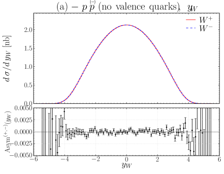
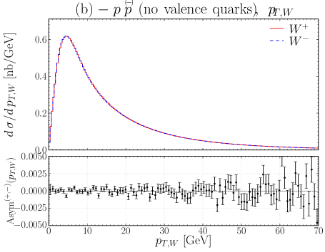
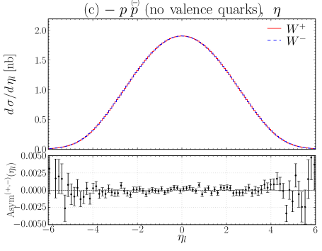
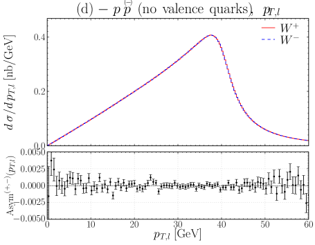
Here let us emphasise the charge symmetry is perfect, by that we mean that in a given point of the phase space the associated infinitesimal cross sections and are exactly equal. This allows us to get rid in the rest of the discussion.
Nonetheless, let us mention that the difference in the PDFs distributions induce an asymmetry between the left and right polarisation states of the . Indeed, as can be seen in Fig. 5.13 the leptons preferentially decay in the direction of the momentum of the which means –using helicity conversation rule of thumb– that and . This can be understood by considering the four main contributions to the production. If we ignore the negligible contributions involving the flavour we are left with : , , , . In the case the quark possesses in general a higher longitudinal momentum than the quark it enters in collision with which means . On the other hand in the cases , and , it is the other way around222To a good approximation for we have except for where ., i.e. which means now . This hypothesis is proved when looking at the individual behaviour of these four contributions in Fig. 5.13.(b), where, to fit the present range in coordinate, the and contributions are respectively multiplied by factors and . Actually this shows the predominance of right is essentially the consequence of the dominating -terms that overrule the other ones.
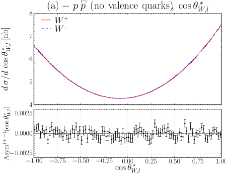
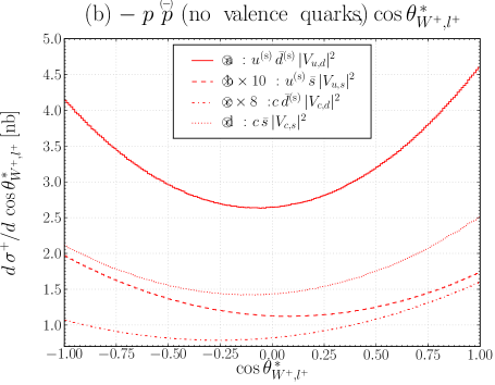
Also worth mentioning is the angle which is not, as displayed by Fig. 5.14, flat along the whole range. The reasons for that comes from the coupling of the leptons to the and to the presence of non-zero and asymmetric of the colliding quarks. Still the explanations to amend this pattern is reported to the study of the and collisions since in those cases the effects are much higher and then easier to explain (note the important zoom in coordinates show the distribution is actually quite flat). The important point here is that just like for there are no charge asymmetries which means no impact for a study of .
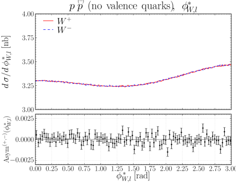
5.A.3 Proton–anti-proton collisions
Now we review the collisions mode reminding the features that makes it perfectly symmetric between the production of and . Let us remind that in our conventions the proton impinges in the direction while the anti-proton does from the direction.
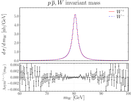
First we turn our attention to the invariant mass of the positively and negatively charged as shown in Fig. 5.15. Note these invariant masses are to be understood as the result of the production of bosons as Breit–Wigner resonances weighted by the PDFs, which adds up to the former behaviour the probability of occurrence of a given mass . Hence, even if here such an equality is non trivial and has to be seen as the consequence that and are produced with the same dynamics in the very particular case of collisions.
The observables , , and are shown in Fig. 5.16. In collisions the production of the and of the are produced with the same dynamics since to every element of the phase-space of, say the , exists the perfect match in an other phase-space point of . This symmetry translates in coordinate space into that the and kinematics are the same up to a vertical flip with respect to the interaction point. This behaviour can be seen in the and distributions but is no longer decipherable when projecting the or the charged lepton transverse momenta on the transverse plane. Note in the and distributions the labels and attached to the data. Focusing on the main “valence” term , in each of these regions the are produced respectively via and for which the inequality materialises the fact that since we have
| (5.15) |
This last inequality explains the presence of the exact same asymmetry for the case of the production.
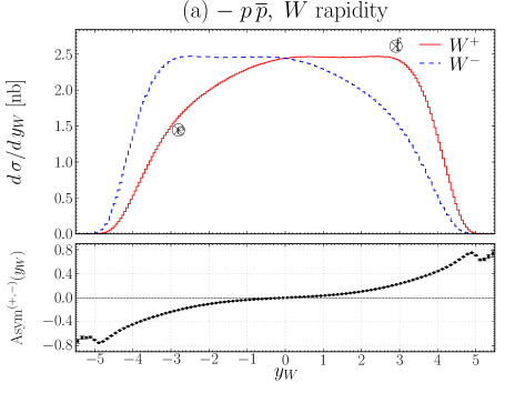
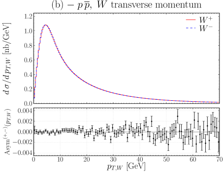
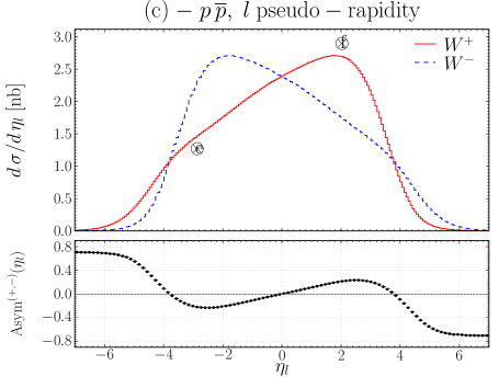
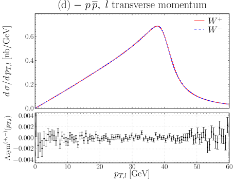
The angular distributions of and are shown in Fig. 5.17. We start by looking at . Both and distributions are superimposed and display a small asymmetry with respect to the origin. This pattern can be explained by focusing on the and the two labels and attached to it in Fig. 5.17.(b). The configurations where the are produced via are such that the will decay preferentially in the opposite direction of the momentum. In the cases where the boson is produced like the will decay preferentially in the same direction of the momentum. Then, the pattern shares the same origin than the asymmetries seen in the and distributions and written in Eq. (5.15). Previously, while studying the pure sea contributions, the inverse unbalance was observed, but now the main “valence” term overrules the latter.
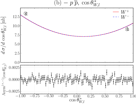
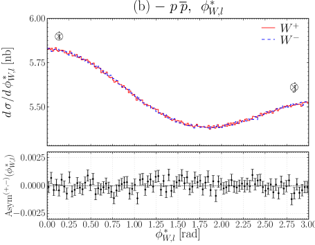
Now even more interesting is the fact that Fig. 5.17 shows and preferentially decays in the same direction of which, as we know, must have dramatic consequences on the smearing of the distributions. Before explaining what happens we take a step back to the LO order and understand how the lack of transverse motion in this approximation induce no asymmetry in the azimuthal decay of the leptons. Figure 5.18 shows the collinear quark–anti-quark collisions of (left) and (right). In both cases the valence quarks hold most of the longitudinal momentum and the privileged direction of decays of the positively and negatively charged leptons (symbolised in the RF) which, even if opposite with each other, do not induce any anisotropic behaviour in .
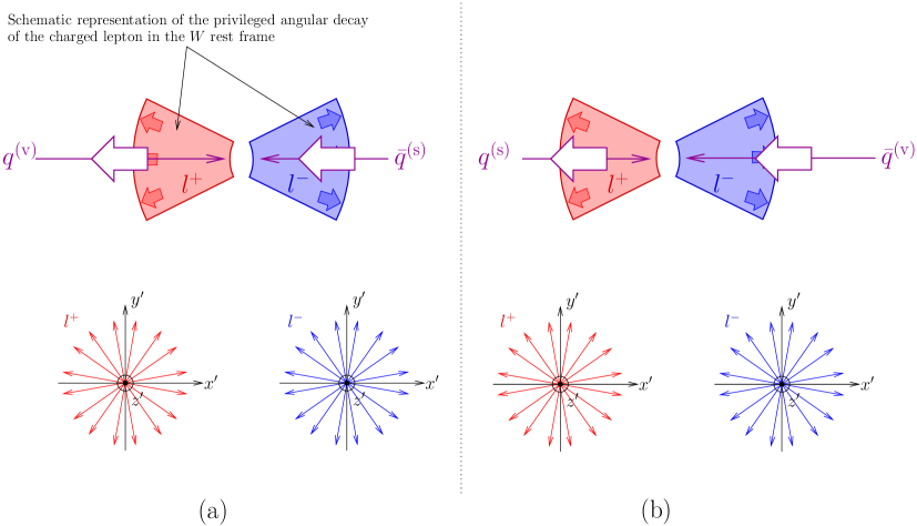
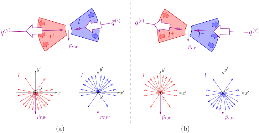
Moving to the improved leading order picture, now quarks and anti-quarks possess a transverse initial motion and radiate gluons and photons on their way to the collision. We end up this time with “valence” cases with the valence (anti-)quark that bears most of the longitudinal momentum and on the other side the sea (anti-)quark which bears most of the transverse motion. In this context the higher transverse momentum of the sea (anti-)quark constrain the leptons to modify their privileged decaying angle to satisfy the kinematic momentum conservation as shown in Fig. 5.18 Hence for events the decays preferentially along the direction of while the decays preferentially in the opposite direction of . In the case of it is the exact opposite. Now, in the context of the production, focusing again on the main “valence” term Figure 5.19.(a) translates to while (b) translates to . Because of the inequality (Eq. (5.15)) (a)-cases overrule (b)-cases and the prefers, in general, to decay in the direction of . The same argument can explain the asymmetry observed in the negative channel. So far, while the fact the valence (anti-)quark hold most of the longitudinal momentum is well known, we did not justified the fact that the sea (anti-)quark hold most of the transverse motion. The very last section of this Appendix address this issue. For now we can justify it heuristically by stating that the sea (anti-)quark having a small fraction is the result of the loss of energy on the way to the collision by gluon/photon emission which confers to the (anti-)quark more transverse motion than the valence (anti-)quark.
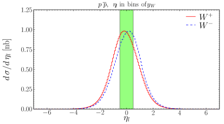
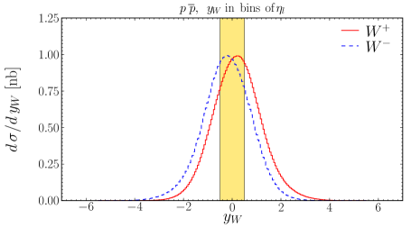
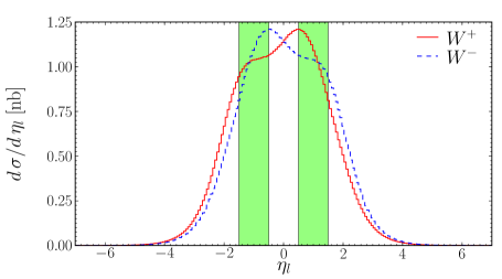
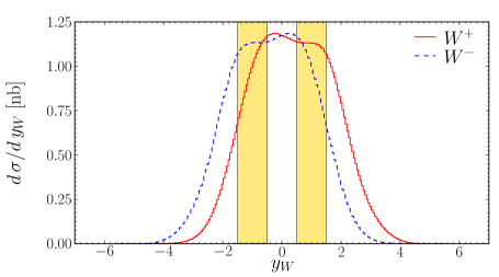
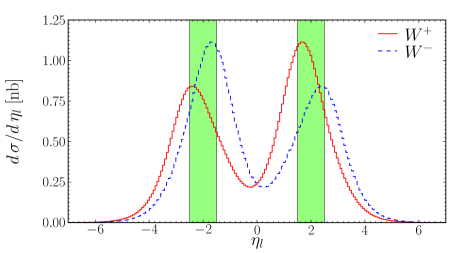
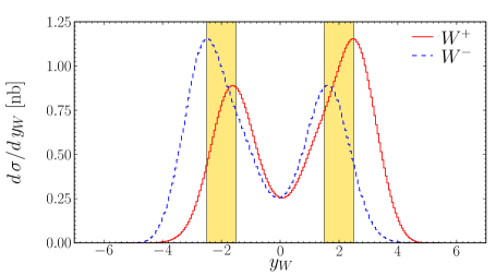
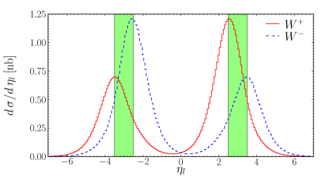
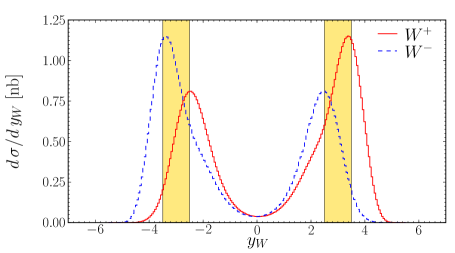
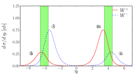
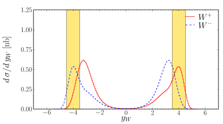
Figure 5.20 by showing the distribution in bins of and vice versa illustrates the importance of the “valence” contributions in function of the fraction of momentum . Starting with in bins of (left) we see the pseudo-rapidity distribution is the addition of two quantities : (1) the rapidity inherited from the boost and that confers to the charged lepton most of its longitudinal motion and (2) the decay of the charged lepton governed by the coupling of leptons to which eventually gives this bump representing the angular coverage of the charged leptons . Let us remind participates in the shape of (2) but can be neglected in this discussion since . In the narrow central bin region where all events verify the small charge asymmetry is due to non-negligible “valence” quark contributions. As the selection in rapidity increases, the “valence” contributions rise displaying in consequence large charge asymmetries in the lepton decay for a local value of . Turning to , for the negative values of the “valence” contributions give bosons while give bosons. The “valence” terms contribute then in both cases to produce right bosons, which imply the decays preferentially in the same(opposite) direction of the momentum. Going to the positive value of is achieved by taking the transformation of the previous example, this time we have giving bosons and bosons. Note that considering at the same time those two opposite -phase space regions completely reestablish the equivalence in the dynamic production of the and the bosons which, using the label notation, would write .
On the right of Fig. 5.20 the distributions in bins of hold more or less the same information than the previous plots. Here though, looking at the variable allows to look at the smearing of the distributions from the boost point of view while earlier the smearing was essentially the one arising from the coupling of the charged leptons to the . Also now we can see that a given slice of receives contributions from an important range of different rapidity. Although it is not important here as no collisions can be made at the LHC it will give insight for LHC collisions at which level the narrow selection in our analysis are contaminated by high rapidity region and hence from “valence” contributions.
Finally we show the behaviour of the “valence” contribution in bins of from the point of view of and in Fig. 5.21 where both charged channels show the same behaviour with almost no asymmetries in because of the negligible “valence” contributions. As the “valence” contributions increases with the selection in rapidity we see that the supremacy of left(right) which was observed inclusively with is back in Fig. 5.17.
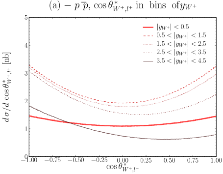
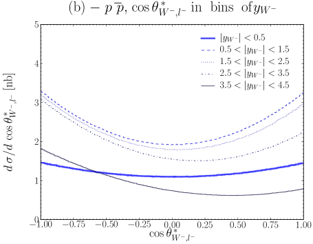
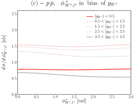
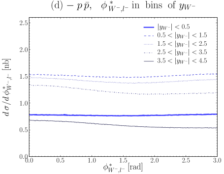
5.A.4 Proton–proton collisions
As we have seen previously even in the case of the collisions there are different asymmetries appearing in the decay of the lepton but eventually no charge asymmetries are observed. Here in collisions, the absence of anti-quarks of valence will open the door to the previous asymmetries to fully express themselves and create important asymmetries between the positive and negative kinematics, especially in the final state.
First of all, before looking at the boson and charged leptons kinematics in specific domain of the phase-space we quantify the global charge asymmetry at the inclusive level due to the fact that in overall we produce more than . Taking the numerical values of the inclusive cross sections for collision (Table 5.1) and writing the global charge asymmetry we evaluate it like
| (5.16) | |||||
| (5.17) |
Then, when looking further one at the discrepancies between the two charged channels in the observable via , all deviations from the horizontal axis have to be understood as the result –in the considered point of phase space– of dynamic issues creating noticeable differences between the positive and negative kinematics in top of the global larger production of with respect to .
This remark can be applied to the very first example in Fig. 5.22 where we can see the peak of the invariant mass of the is slightly centered to a higher mass than the one of the . We observe . Let us emphasise this behaviour is already present at LO. We explain this effect heuristically with the following idea. In the quark–anti-quark collision the more energy is brought, the more the mass of the can take its share for its mass . The cases which fall under this category are the one involving a valence quark, for a , and a valence quark for a . Since in general quarks carry more longitudinal momentum than the quarks it turns out they have more opportunities to participate to the production of a high mass . Hence, eventually, at the hadronic level are produced with higher masses with respect to the .
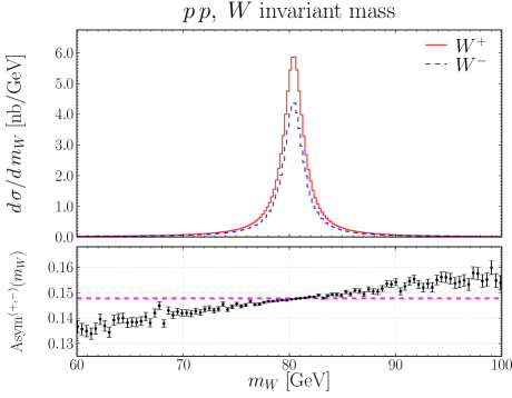
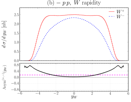
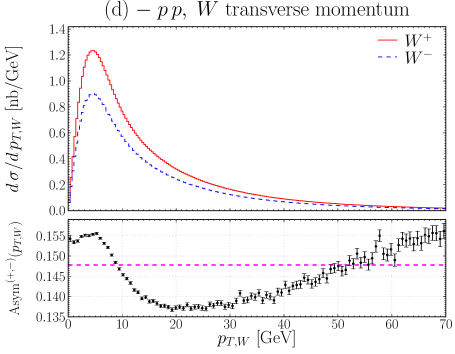
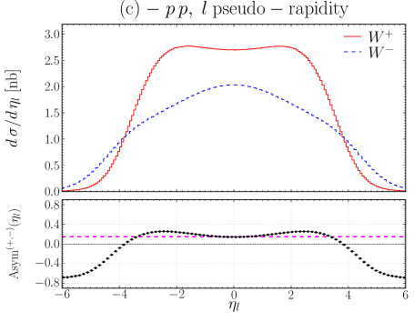
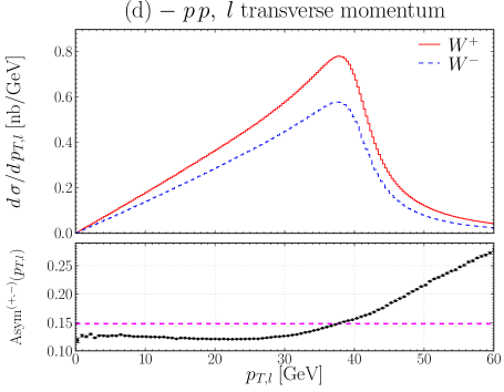
Figure 5.23 shows now the kinematics of the bosons and of the charged leptons. The rapidity displays two striking features, the first and most trivial, is a difference in the scale which simply relates that we have roughly twice many than in collisions. The second feature shows the rapidity extends to a wider range than the which means the can gain a more important longitudinal motion than the which is the consequence than the quarks carry most of the proton momentum. The charge asymmetries in comes from the difference in the production of the and . Because of the important implications in terms of systematic errors in the study of this specific topic was discussed in the core of the Chapter (cf. § 5.2). Turning now to the charged lepton kinematics we observe that the pseudo-rapidity distribution follows roughly the pattern of the rapidity with the particular feature that the tends to decay in the direction of the momentum direction while it is the inverse behaviour for the . This pattern will be detailed further while looking at the distributions in bins, at this stage we can already understand that the excess of matter in collisions implies
| (5.18) |
To the light of the known behaviour of the charged lepton in their decay under the constrain of the coupling in EW interactions, this explains respectively the narrowing and flattening of the and distributions. This can be seen more directly in Fig. 5.25.(a) looking at the distributions. To the purely sea pattern seen in Fig. 5.13.(a), we add up the “valence” terms but consider for simplicity in the discussion only the main term for the and for the . Events such as give bosons from which the leptons decay preferentially in the opposite direction of materialising eventually as in the Figure. For bosons, this time create bosons from which the leptons decay most of the time in the direction of . Eventually the inequality in the gaps “” “” is explained once again by , i.e. from the common pattern of the purely sea contribution the predominance of quarks in the collision adds up a larger asymmetry in relatively to the one for .
Coming back to the charged lepton kinematics the transverse momentum of the charged lepton shows very important charge asymmetries. The sources for those are : (1) , (2) and (3) the non isotropic azimuthal decay of the charged leptons with respect to the direction of feature which has been already discussed in the case of collisions. The first source cannot be the one responsible for the size of these effects. Figure 5.24 proves it by showing at LO where is already present while (2) and (3) are not, and at the improved LO where all three effects are present.
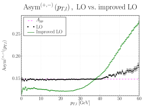
The reason for these large asymmetries in the distributions is explained by the predisposition of the leptons to decay preferentially in the direction of while it is the over way around for the leptons. This can be seen directly in Fig. 5.25.(b) showing the distribution. The explanations of this effect can be followed looking at Fig. 5.19, where this time the total absence of the (b) contribution involving valence anti-quarks open the door to effects (a) to fully express their charge dependent discrepancies. We start by addressing the case of the through the main “valence” term where, the higher transverse motion held by the forces the to decay most of the time so that . The case of the is identical but this time the opposite helicity of the makes it so it decays preferentially in the opposite direction of , i.e. . Once again the relative size of the “” and “” gaps is justified by .
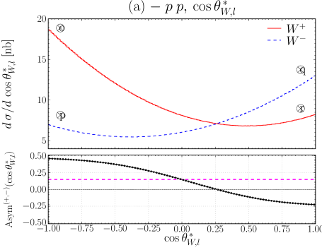
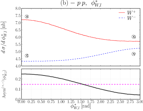
Figure 5.26.(left) allows now to see the difference in the behaviour of the decaying leptons in bins of through their pseudo-rapidity. Just like in collisions the asymmetry due to the “valence” contributions is almost negligible in the central narrow selection and then rise with the rapidity except that this time the asymmetries are not matched between and when summing the two opposite slices contributions but rather magnified. In the case of , the excess of is such that in average most of the leptons decay in the opposite direction of as shown by the bumps in and . On the other hand the , due to the excess of , follow the bosons momentum direction as displayed by the and bumps.
This large influence of the valence quarks in the high rapidity region suggests that for a measurement of , selecting charged leptons emitted from low rapidity would at least allow to reduce the systematics uncertainties related to the valence or sea quarks. By going to the narrow region one can see the size of the “valence” contamination in this region is non negligible. This is the reason why in the core of the Chapter the narrow selection was made rather to since it was found to be the best compromise for a realistic measurement prospect in Chapter 6.
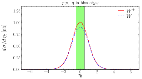
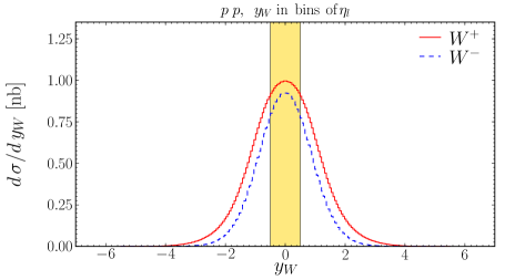
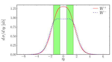
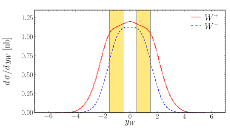
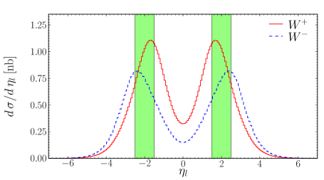
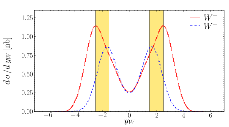
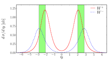
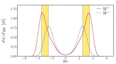
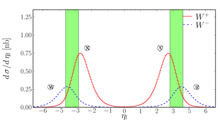
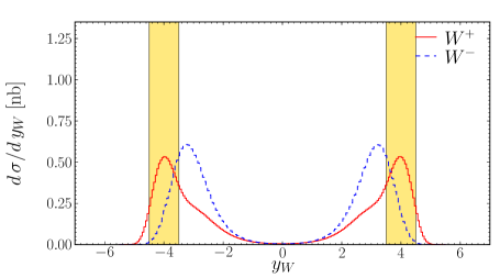
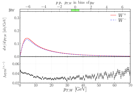
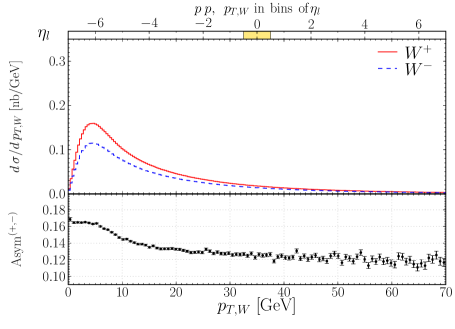
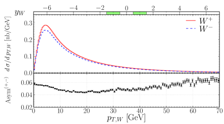
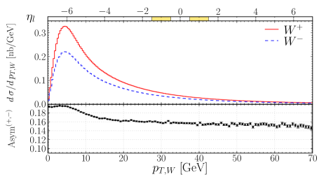
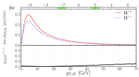
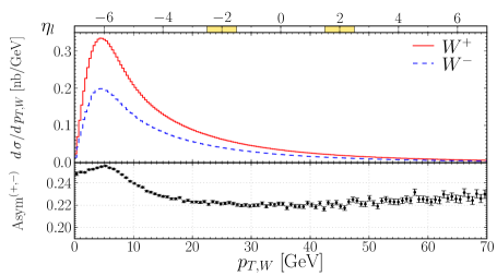
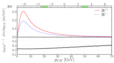
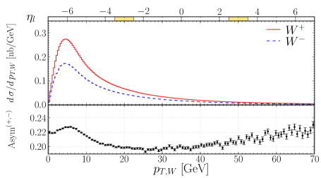
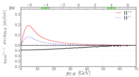
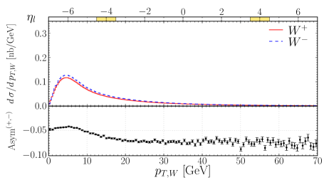
Figure 5.27 shows the size of the initial state charge asymmetries by looking at the transverse momentum of the boson.
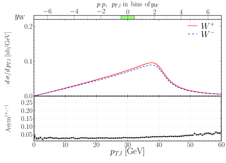
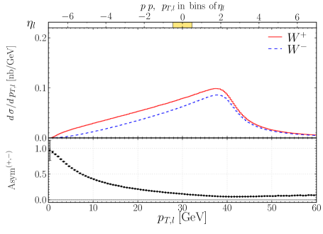
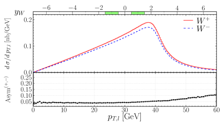
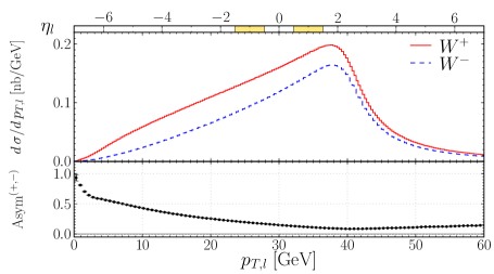
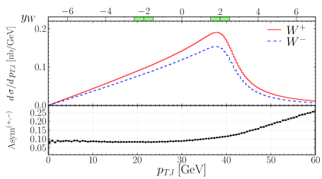
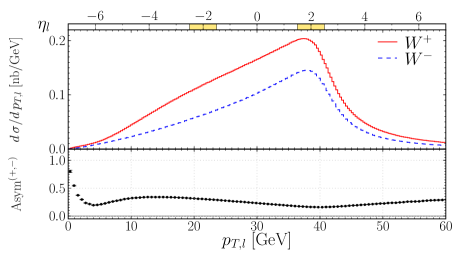
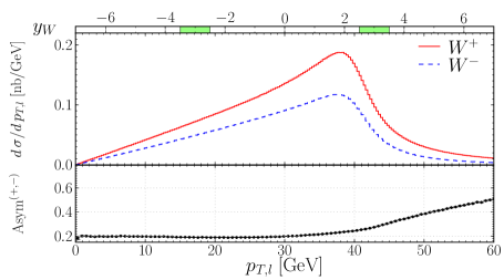
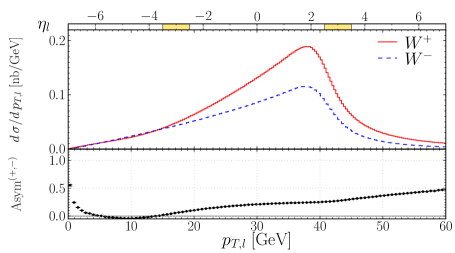
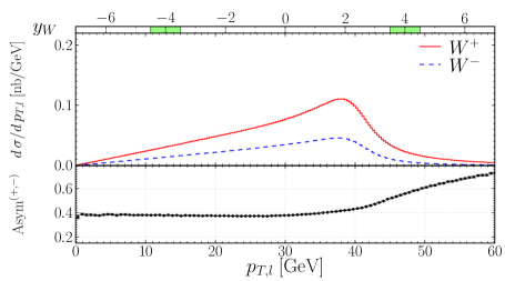
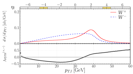
Figure 5.28 shows the increase of the final state charge asymmetry in bins of and .
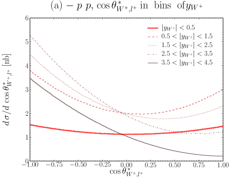
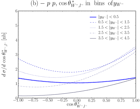
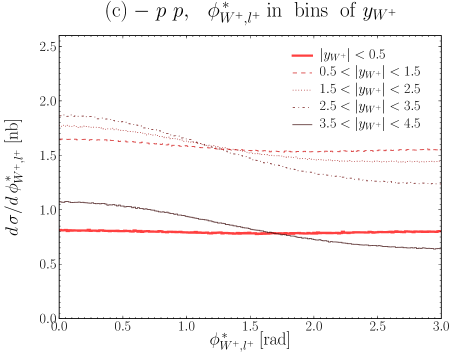
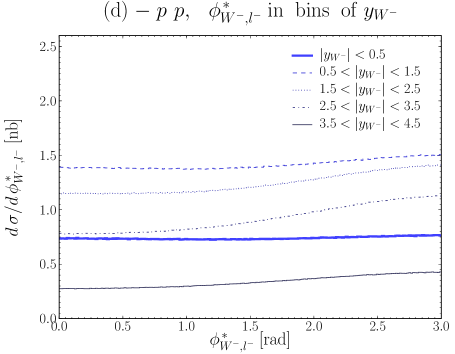
Another vision of the growth of the “valence” contributions in function of can be made looking at the and distributions in bins of (Fig. 5.29). In the central region the asymmetry between left and right is hardly decipherable (contrary to the same phenomenon seen in -space).
5.A.5 Deuteron–deuteron collisions
Here, the overall charge asymmetry based on the inclusive cross sections from Table 5.1 gives
| (5.19) |
The predictions for collisions can be understood from the previous study of collisions. Indeed, here the novelty is that reaching the equality allows to cancel out the most important differences between the and at the level of the production.
The invariant masses of the and in Fig. 5.30 are now superimposed up to the very small offset. Hence here the and masses occur with almost the same probabilities, we find .
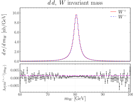
Concerning the main kinematics , , and shown in Fig. 5.31 the most striking feature is the gain of charge symmetry in the initial state with respect to collisions. Because now the production of the and is almost the same in proportions the rapidity and transverse momentum distributions almost perfectly match each other. On the other hand in the final state the effect folded to the issues related to the transverse motion of the gives unchanged features such as : (1) the flattening of the and narrowing of the distributions with respect to and (2) the privileged decay of the () in the same(opposite) direction of . These two effects can be seen respectively more directly from the angular point of view with and in Fig. 5.25. Let us note as well the size of which is different from collisions. This is due to the energy in the collision which, being lower here, gives more importance to the valence quarks while at the latter are drowned in the large purely sea contributions. This variation of as a function of is treated in the next sub-section.
Figure 5.33 shows the distributions in bins of and vice versa. Note the charged leptons behaviour are the same than in collisions but now the proportions of and are the same, which is particularly noticeable in the last two lines where the positive and negative -pieces of the plots do not interpenetrate each other. Figure 5.34 shows the transverse momentum of the in bins of and . As can be seen, even if here the discrepancies are induced by the , and flavours since they are weighted by the valence quarks (Eq. (5.3)) it is in the forward rapidity region they are the most important. Figure 5.35 displays the charge asymmetry of the charged leptons transverse momenta in bins of (left) and (right). Again we observe the growth of the charge asymmetry as increases and in general using a crude selection we witness a rather poor correlation with respect to the reference selection results. The and distributions in bins of are presented in Fig. 5.36.
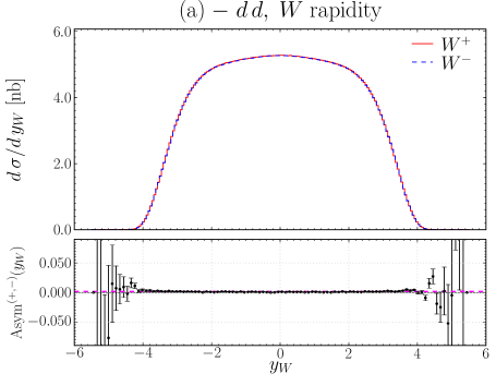
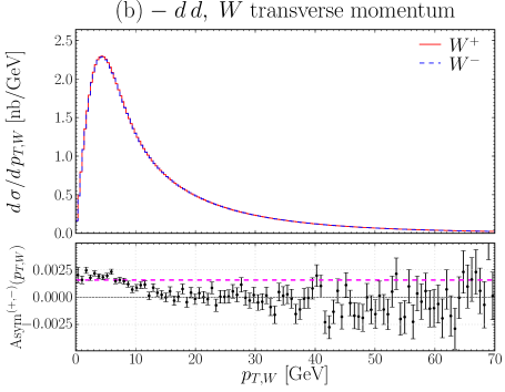
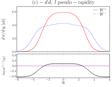
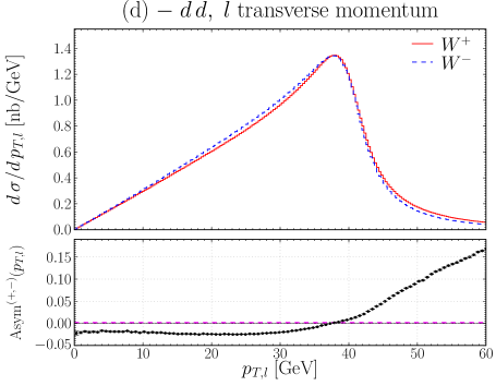
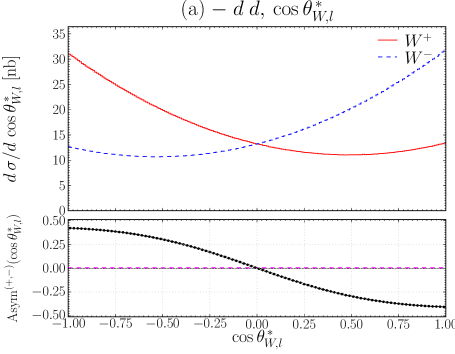
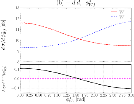
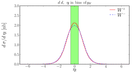
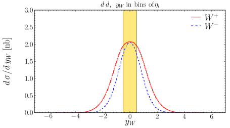
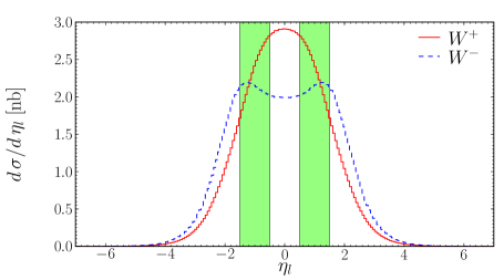
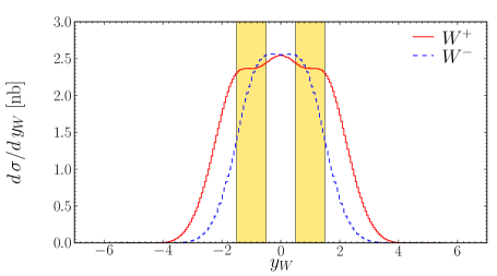
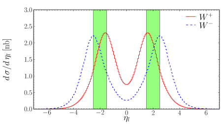
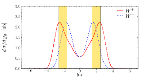
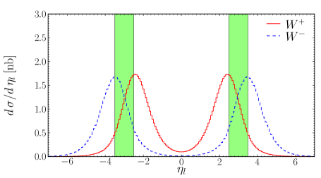
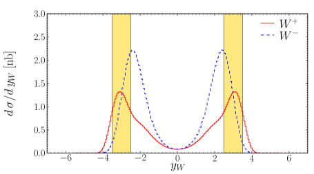
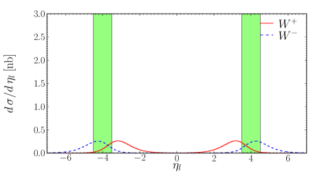
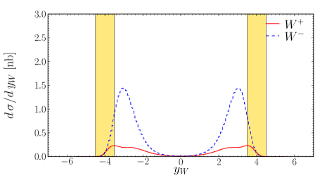
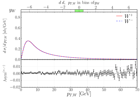
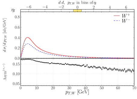
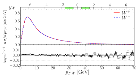
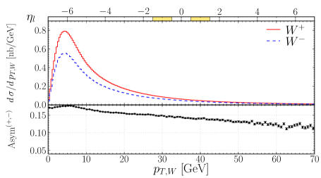
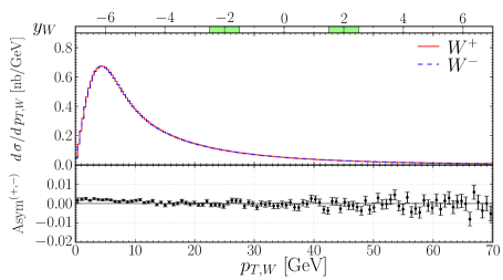
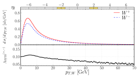
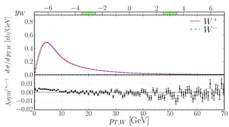
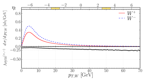
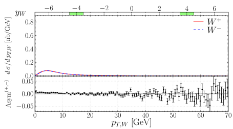
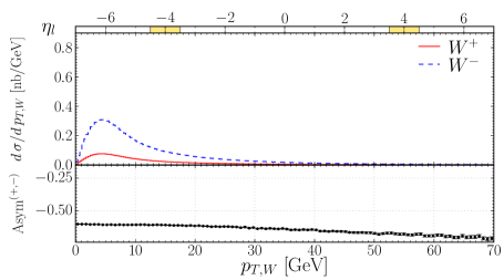
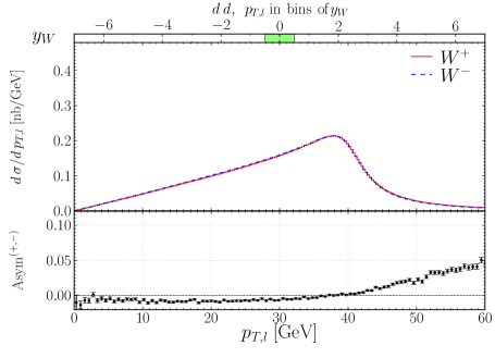
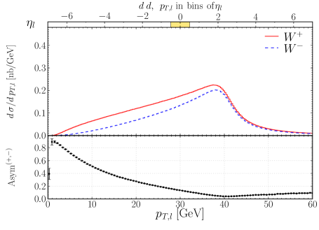
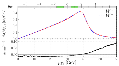
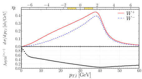
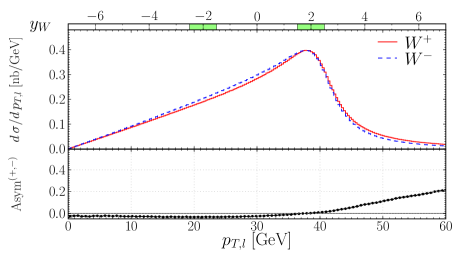
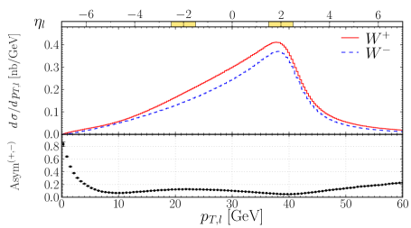
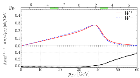
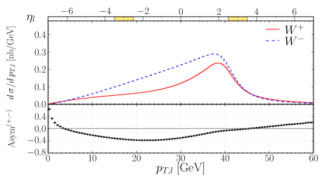
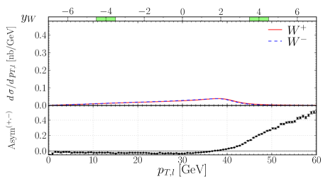
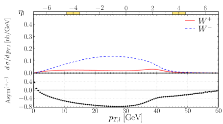
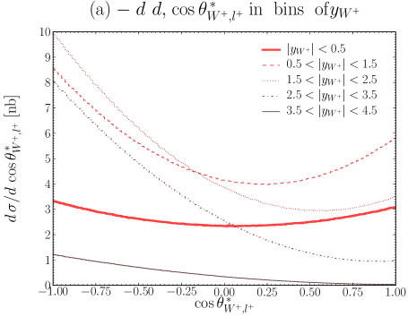
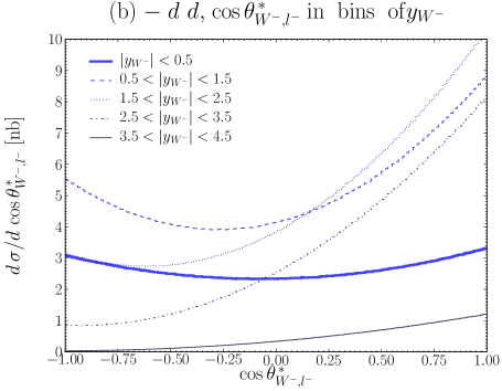
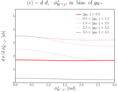
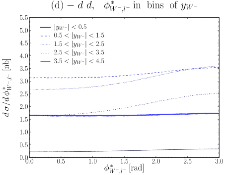
5.A.6 Transverse momentum of the (anti-)quarks for in Drell–Yan
This sub-section presents more explanations on the transverse momenta unbalance between the valence quark and the sea anti-quark.
In most cases the valence quarks brings most of the energy in the collision. These configurations with high for the valence quark and low for the sea anti-quark are already well know. Now the thing is that a parton with a small will have in general a higher transverse motion gained on its way to the collision by radiating gluons and photons (note also the low (anti-)quark can be as well the product of the radiation of a gluon via ).
Finally because of the CKM missing angles the other flavours such as , and have their transverse motion influenced as well. To emphasise this aspect let us note that in the case of the production of bosons since the previous flavours create bosons only via annihilation we observe in those specific cases (we used for that the generator WINHAC which as said earlier can produce bosons, cf. § 4.1.2).
The previous ideas are illustrated in Fig. 5.37 with the histograms of the inclusive transverse momenta of the and flavours in the production (a) and the one of the and flavours in the production (b). In both cases the sea quark show larger probability to hold a high while the valence quark hold a low . These histograms were obtained, like the others, for a statistic of millions of weighted events.
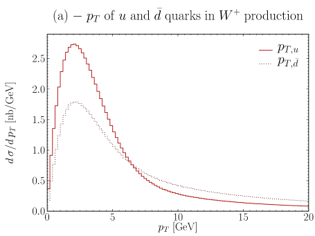
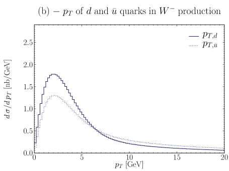
The corresponding estimation of the average of the and quarks are
| (5.20) | |||||
| (5.21) |
Anyhow in the previous values and values intervene, to factorise in a better way the asymmetries induced by the cases where there is a valence quark involved in the collisions we repeat the previous study putting to zero the sea contributions and , in that context, the average of the quarks in “valence” contributions for production of
| (5.25) |
and for “valence” contributions in production of
| (5.28) |
In both cases we observe that the valence quark holds a very low transverse motion with respect to the anti-quark. Note also that the transverse motion of the sea anti-quark increases with the mass of the quark.
Now these average of the quarks for purely sea contribution are :
| (5.32) |
for the production. Because for we observe while it was the other way around for “valence” contributions. Also let us remark again that the higher the mass of a quark is the higher its transverse motion is. In the case of the production we have
| (5.35) |
Let us remark that averaging the “valence” and purely sea contributions does not give exactly the values estimated when taking all contributions. This can be explained by the fact the proton’s integrity cannot be exactly factorised into “valence” and purely sea contributions.
5.A.7 Amplitude of the final state charge asymmetries in function of the energy in the collision
As observed in the study of deuteron–deuteron collisions the final state charge asymmetries in the observable is larger than for the case of proton–proton collisions. The energy in the collision is the parameter responsible for those effects. To see how this works we study as a function of the energy in the center of mass frame (Fig. 5.38.(a)). As increases we witness the decrease of the charge asymmetry. Knowing the charge asymmetry comes from “valence” contributions as the energy rise the charge symmetric purely sea contributions increases and we end up with a lower and lower proportion of asymmetry due to “valence” terms. Nonetheless, the asymmetry in the quarks for “valence” contributions increases with . We find for example in the two extreme cases and the nominal collision mode :
| (5.36) | |||||
| (5.37) | |||||
| (5.38) |
To emphasise the increase of the asymmetry in absolute as grows we look at the bare difference of the positively and negatively charged histograms. This is shown in Fig. 5.38.(b), the purely sea contributions giving exactly the same contributions we are left with the difference between the “valence” terms only.
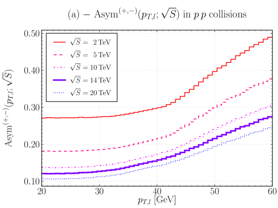
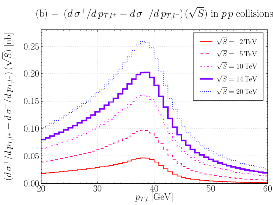
Anyhow, the important idea here is to understand that the energy in the collision which is lower in the hypothetical case of collisions runs at the LHC forces us to deal with larger charge asymmetries with respect to the seen in collisions runs. This will explain the different behaviour of the systematic analysis prospect between and collisions in the next and final Chapter.
Chapter 6 Strategy for a reduction of the systematic errors on
“But then …” I venture to remark, “you are still far from the solution. …”
“I am very close to one,” William said, “but I don’t know which.”
“Therefore you don’t have a single answer to your questions ?”
“Adso, if I did I would teach theology in Paris.”
“In Paris do they always have the true answer ?”
“Never,” William said, “but they are very sure of their errors.”The Name of the Rose
Umberto Ecco
Here we finally present the dedicated strategies that were devised –based on the knowledge built throughout Chapter 5– to prepare a measurement of at the LHC. As already mentioned in the first Chapter while at the Tevatron the statistical and systematic errors where of the same order at the LHC the first one will drop to for just one year of harvesting data at low luminosity. On the other hand the systematic error will be still important and we show how using the LHC and ATLAS detector capabilities we could eventually decrease those systematic errors and thus enhance by a factor the actual precision on . The most important results below were presented in Ref. [146].
The Chapter is divided as follow. The first Section presents the strategies and observables developed in our collaboration which, according to us, should be more robust to address this particular measurement at the LHC. Following that a presentation of the general context for studying in Drell–Yan is briefly reminded. The second Section describes the principle of the analysis to extract the mass parameter for both the classic and the new suggested methods. The third Section addresses the sources of theoretical and experimental systematic errors that should be taken into account in the estimation of the error on this measurement. Finally in the last Section our strategies robustness with respect to both theoretical and apparatus unknowns addressed in our analysis are improved on the example of the simulation of one year of data taking at low luminosity.
6.1 Measurement strategies
6.1.1 Event selection
As mentioned earlier the extraction of the and bosons properties is achieved by studying their electronic and muonic decays, that is respectively and . The choice for leptonic decays is motivated by the fact the di-jet background is of several orders of magnitude more important than the and signals we would be interested in while the leptonic decays provide clean processes (i.e. absence of QCD in the final state) with large cross sections. The decays to the tau channel is not considered though because the mass of the charged is such that it decays within , which leads to at least two neutrinos to deal with for the detection of the final state.
The particular study of the and bosons is made by splitting the data collected for the bosons into positively and negatively charged leptons in the final state to get the corresponding and data. The main criteria used in hadronic collider to study bosons are to have a high energy charged lepton in the high precision detector volume of the detector associated with high transverse missing energy that betrays the presence of the neutrino. Also, to reduce the background, rejection are made using constraints on the recoil defined as the sum of all momenta recoiling against the system
| (6.1) | |||||
| (6.2) |
but again, due to the non possibility to measure the longitudinal component of the particles escaping the beam-pipe, its transverse component is considered instead.
From the total number of events produced inclusively (Eq. (3.5)) now must be taken into account the effects of the acceptance selection, the reconstruction efficiency and the background processes whose kinematics can lure the trigger to recognise them as lepton pair decaying from single . Taking that into account, eventually the number of candidates from Drell–Yan are
| (6.3) |
where is the number of accepted events by the cuts and is the number of background events. The expression of reads
| (6.4) |
where the integrated luminosity, the cross section that the events fulfill the selection requirements and is the efficiency reconstruction for the signal in the given fiducial region. The number of background events can be expressed like
| (6.5) |
where is the cut cross section of all the processes that displays kinematics in their final state that mimic the features of the final state leptons from Drell–Yan and is the contribution term due to the electronic noise, the cavern background, etc. Below, more details on these criteria are given for the case of CDF, ATLAS and finally for our stand-alone analysis prospect.
Event selection in CDF.
In CDF II [51] a Drell–Yan is recognised by having at least one lepton candidate in the central region () and by applying the following narrowing selection on the kinematics :
-
-
The charged lepton must verify : .
-
-
The neutrino , deduced from the measurement of , must verify : .
-
-
The leptons transverse mass must verify :
-
-
The transverse recoil must verify : .
Additional cuts are made to reject background from leptonic decays. Eventually the measurement of the properties in Ref. [51] based on these selection criteria provided candidates events for () and candidates events for ().
Expected event selection in ATLAS.
In ATLAS, although no data is there yet to confirm which criteria would fit the best the LHC context the adopted requirements taken from Ref. [71] are :
-
-
Have a charged muon or isolated electron with in the precision physics acceptance volume ().
-
-
Have a missing transverse energy of .
-
-
No jets in the event with to reject backgrounds from jets and events.
-
-
A recoil to avoid to much the influence of the smearing on the leptons. observables
In ATLAS, these constraints should be such that from the millions of bosons produced for an integrated luminosity of only millions should be accepted (no matter the charge or the decay channel).
Event selection for the present study.
The boson production events used in our studies are selected by requiring that the simulated decaying charged electron or muon satisfy the following requirements :
| (6.6) |
We assume that by using a suitable cut the impact of the uncertainty in the background contribution on the measurement of the charge asymmetry of the boson mass at the LHC can be made negligible. This allows us to skip the generation and simulation of the background event samples for our studies. It has to be stressed that the above assumption is weaker for the measurement of the charge asymmetry than for the measurement of the average boson mass [57, 58] because, to a good approximation, only the difference of the background for the positive and negative lepton samples will bias the measurement. The presentation of the results of our studies is largely simplified by noticing that they are insensitive to the presence of the cut in the signal samples. Therefore, the results are based on selection of events purely on the basis of the reconstructed charged lepton kinematics variables as shown in Eq. (6.6). Studies have shown that these results will remain valid whatever cut will be used at the LHC to diminish the impact of the background contamination at the required level of precision. To be more precise, in our simple model this cut was emulated by a direct cut. Nonetheless, in the specific purpose of a cut, this approximation is believed to be fully justified.
The detector response is based on the ATLAS tracker which, for reminder, was emulated using Gaussian resolutions for and of the charged electron and muons according to Eqs. (3.15–3.16).
Concerning the statistic, in absence of background and imperfect reconstruction efficiencies, we simply have
| (6.7) |
The cut cross section corresponding to the requirements of Eq. (6.6) and for the expected LHC energies for (Eq. (3.11)) and (Eq. (3.12)) collisions are compiled in Table 6.1. Table 6.2 gives the correspondence in terms of number of events obtained by using the respective integrated luminosities for and collisions (Eqs. (3.11–3.12)) in Eq. (6.7).
| Collisions | [nb] | [nb] | [nb] | [nb] | [nb] | [nb] |
|---|---|---|---|---|---|---|
| Collisions | ||||||
|---|---|---|---|---|---|---|
6.1.2 Observables
The values of the and boson masses can be unfolded from the measured lepton charge distributions , and from the transverse mass . We discuss only the methods based on the measurement of . These methods are almost insensitive to the detector and modeling biases in the reconstructed values of the neutrino transverse momentum . We are aware that, for the measurement of the average mass of the boson, this merit is outbalanced by the drawback of their large sensitivity to the precise understanding of the distribution of the boson transverse momentum (Fig. 2.15). However, for the measurement of the charge asymmetry of the masses this is no longer the case because QCD radiation –which drives the shape of the distribution– is independent of the charge of the produced boson. In our view the based methods will be superior with respect to the based ones, in particular for the first measurements of the mass charge asymmetries at the LHC.
(a) Commonly used observables
In the context of a based method for the extraction of , the most natural method is to analyse separately the and event samples and determine independently the masses of the and bosons. This method, that will be investigated, is based on independent measurements of the and distributions. It will be called hereafter the classic method and actually corresponds to what physicists did at with the CDF detector to provide measurements of .
(b) The charge asymmetry
A new method proposed and evaluated in our collaboration is based on the measurement of the charge asymmetry (Eq. (2.13)) of the distribution. This method will be called hereafter the charge asymmetry method. The distribution of is, by definition, robust with respect to those of systematic measurement effects and those of model dependent effects that are independent of the lepton charge. The acceptance, and the lepton selection efficiency corrections for this observable will, in the leading order approximation, reflect only their lepton charge dependent asymmetries. In addition, the observable is expected to be robust with respect to the modeling uncertainty of the QCD and QED radiation processes.
If extrapolated from the experience gained at the Tevatron (cf. Appendix 3.A), the precision of the charge asymmetry method will be limited by the understanding of relative biases in the reconstructed transverse momenta for positively and negatively charged particles (cf. § 3.4). These biases, contrary to the lepton charge averaged biases, cannot be controlled using the , and “standard candles” that helps only to correct for the absolute energy scale. This problem leads us to the third and final observable for our study : the double charge asymmetry.
(c) The double charge asymmetry
The double charge asymmetry is defined like
| (6.8) |
where the variable defined like (cf. § 2.3), represents the radius of the track curvature at the boson production vertex in the plane perpendicular to the beam collision axis and is the strength of the solenoidal magnetic field bathing the inner tracker. The choice on was cast to follow the notation adopted in our former work [145]. The measurement method using the distribution will be called hereafter the double charge asymmetry method.
The distribution is expected to be robust with respect to the charge dependent track measurement biases if the following two conditions are fulfilled : (1) the inversion of the -component of the magnetic field in the tracker volume can be controlled to a requisite precision and (2) the Lorentz drift relative corrections to the reconstructed hit positions for the two magnetic field configurations, in the silicon tracker could be determined to a requisite precision. Discussing these two conditions in details is beyond the scope of this work. Nonetheless the second point, in view of the ATLAS detector design was considered qualitatively in our work [111] with regard to the specificity of the pixel, SCT and TRT barrel modules.
First, the inversion of the magnetic field should a priori have no influence on the TRT intrinsic capabilities since the measurement of the hit is based solely on the time it takes for electrons to drift to the center wire as shown in Fig. 3.18.(b). Then, reverting the magnetic field should reverse the drift paths of the electron but not affect the drift time. Concerning the SCT barrel modules the tilt angle for the invert magnetic field configuration is now worsening the nominal hit resolution as depicted in Fig. 6.1. In the best case scenario the Lorentz drift angle made by the drifting electrons is well under control and the resolution of the SCT for the inverted magnetic field should be well accounted. If that would not be the case then the resolution of the SCT modules will change. Nonetheless the double layer feature of silicon wafers, by providing an average offline hit position, should help to tackle such problems.
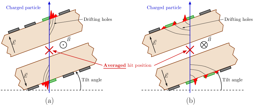
This is no longer the case for the pixel detector whose modules posses only one layer. As seen previously the pixel hits are important as they provide data on the particles before they start to loose energy to the apparatus and also because of the important lever arm they have for the track fitting reconstruction procedure. Here, to each event, looking at the origins of the other particles tracks should help for a possible correction of the production vertex of the leptonic decay.
To conclude, in Fig. 6.2 we show the distributions of and for : (1) the generated and unselected sample of events, (2) the generated and selected sample of events and (3) the unbiased simulated detector response and selected sample of events. The corresponding histograms in -space can be in seen in Figs. 6.7.(a), (b) and (c) of Appendix 6.A. The analysis of the systematic biases affecting these distributions allows to evaluate the precision of the measurement methods discussed in this section.
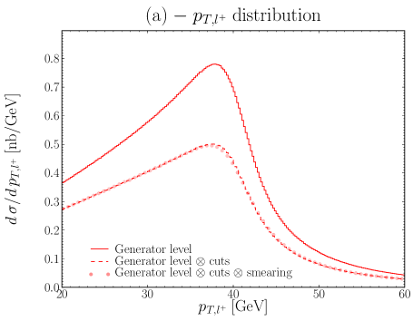
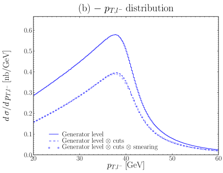
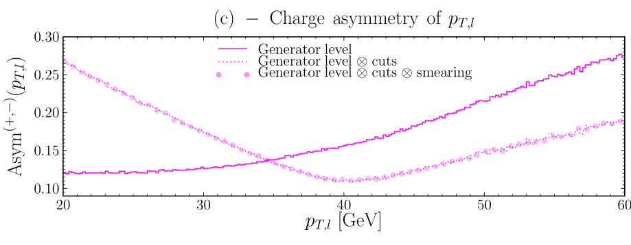
6.1.3 The machine and the detector settings
The primary goal of the ATLAS and other LHC experiments is to search for new phenomena at the highest possible collision energy and machine luminosity. It is obvious that, initially, the machine and the detector operation modes will be optimised for the above research program. The main target presented here is to evaluate the precision of the measurement of the mass charge asymmetry which is achievable in such a phase of the detector and machine operation.
A natural extension of this work is to go further and investigate if, and to which extent, the precision of measurement of the Standard Model parameters could be improved in dedicated machine and detector setting runs. In our first work [145] we discussed the role of : (1) dedicated runs with reduced beam collision energies, (2) dedicated runs with isoscalar beams and (3) runs with dedicated detector magnetic field settings ; in optimising the use of the boson production processes as a “standard candle” for the boson processes. Here some of these dedicate settings were found to be of interest but the most important ones were devised in the particular context of this measurement of . More precisely, we discuss the possible improvement in the measurement precision of the charge asymmetry of the boson mass which can be achieved (1) by replacing the proton beams with light isoscalar–ion beams and (2) by running the detector for a fraction of time with the inverse direction of the solenoidal magnetic field. These and other dedicated operation modes could be tried in the advanced “dedicated measurement phase” of the LHC experimental program. Such a phase, if ever happens, could start following the running period when the collected luminosity will become a linear function of the running time and the gains/cost ratio of its further increase will be counterbalanced by the gains/cost ratio of running dedicated machine and detector operation modes.
6.2 The analysis method
In this section we present the technical aspects of the analysis method used in the evaluation of the achievable precision of the measurement of the charge asymmetry of the boson masses, , denoted sometimes for a matter of convenience .
The shapes of the experimental distribution (generator level cuts smearing) shown in Fig. 6.2 are sensitive to : (1) the assumed values of and , (2) the values of the other parameters of the Standard Model, (3) the modeling parameters of the boson production processes and (4) the systematic measurement biases. Our task is to evaluate the impact of the uncertainties of (2), (3) and (4) on the extracted values of and for each of the proposed measurement methods. It is done using a likelihood analysis of the distributions for the pseudo-data () event samples and those for the mass template () event samples. Each sample represents a specific measurement or modeling bias, implemented respectively in the event simulation or event generation process. Each sample was generated by assuming a specific () value or a value of their charge asymmetry . The samples are simulated using the unbiased detector response and fixed values of all the parameters used in the modeling of the boson production and decays except for the mass parameters. The likelihood analysis, explained below in more detail, allows us : (1) to find out which of the systematic measurement and modeling errors, could be falsely absorbed into the measured value of the boson masses and (2) to evaluate quantitatively the corresponding measurement biases.
6.2.1 Likelihood analysis
Let us consider, as an example, the impact of a systematic effect on the bias in the measured value of the mass determined from the likelihood analysis of the distributions. Since some of the upcoming results were carried based on observable as well we mention already the correspondence in terms of resolution and range.
The simulation of the pseudo-data event sample, , representing a given systematic bias , is carried out for a fixed value of the mass . Subsequently, a set of the unbiased (i.e. ) template data samples is simulated. Each sample of the set corresponds to a given value of
| (6.9) |
with and where for the rest of the document . The likelihood between the binned distributions for the sample and the -dependent sample is quantified in terms of the value :
| (6.10) |
where is the content of the bin of the histogram entering in the analysis and is the corresponding statistical error. In total, bins enters in the analysis, it represents the degrees of freedom (dof), . The bulk of the results presented has been obtained using a bin size corresponding to (respectively ) which is approximately the anticipated measurement resolution of the track curvature [96] and the summation range satisfying the following condition for ()
| (6.11) |
which corresponds to degrees of freedom of (). This choice is justified as the CDF II measurements were realised for the observable in the range to get rid as much of the background by focusing on the jacobian peak region.
The dependence upon is fitted by a polynomial of second order. The position of the minimum, , of the fitted function determines the systematic mass shift due to the systematic effect . If the systematic effect under study can be fully absorbed by a shifted value of , then the expectation value of is and the error on the estimated value of the mass shift, , can be determined from the condition (see Ref. [1] for further details on this topic).
Of course, not all the systematic and modeling effects can be absorbed into the variation of a single parameter, even if the likelihood is estimated in a narrow bin-range, purposely chosen to have the highest sensitivity to the mass parameters. In such cases the value of can be substantially larger than , and looses its statistical meaning. This can partially be recovered by introducing additional degrees of freedom (the renormalisation of the samples, discussed later on in § 6.2.3, is an example of such a procedure). However, even in such a case the estimated value of will remain slightly dependent upon the number of the samples, more precisely their spacing in the vicinity of the minimum and the functional form of the fit. Varying these parameters in our analysis procedure in a -dependent manner would explode the PC farm CPU time and was abandoned. Instead, we calibrated the propagation of statistical bin-by-bin errors into the error, and checked the biases of all the aspects of the above method using the statistically independent “-calibration samples” in which, instead of varying the effects, we varied the values of .
6.2.2 The and event samples
(a) Classic method
In the classic method the bias of resulting from the systematic effects is determined in the following three steps :
-
1.
Determine using .
-
2.
Determine using .
-
3.
Combine these results and derive respectively the central error for and the associated error by adding up quadratically the errors on each charged channel
(6.12) (6.13)
In the generation of the samples we assumed . The samples have been generated for with and for with . In total samples, corresponding to , have been generated. Table 6.3 recaptures in the left column the shifted values from the used to generate both positive and negatively bosons .
This procedure is illustrated in Fig. 6.3 where, for convenience, and just for this specific figure, the extreme mass templates where generated with to make it possible to see the difference between the three distributions. As expected since there is no bias the parabola fit is centered on , more precisely with . The same procedure applied for the negatively charged channel gives the result with . These two results, once combined, give
| (6.14) |
It shows that no systematic biases are introduced by the proposed analysis method and give an idea on the size of the statistical errors.
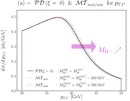
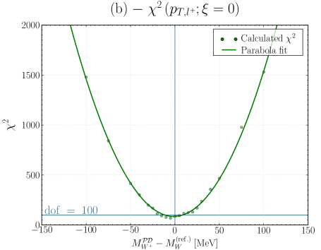
(b) Charge asymmetry method
In this method the biases resulting from the systematic effects are determined by a direct analysis of the distributions for the and event samples. For the samples, combining the event sample and produced shifts for the parameter as shown in the second column of Table 6.3. Even though the basics allowed us to spread the range of the analysis to , most of the values for the systematic errors are such that it proved to be reasonable to stay in the range.
| [MeV] | [MeV] | |
|---|---|---|
In preliminary studies the charge asymmetry method was first verified using two charge symmetric procedures. In the first one the variation of was made by fixing and by changing . In the second one we inverted the role of and . The results obtained with these two charge symmetric methods were found to agree within the statistical errors.
The first measurement of the charge asymmetry of the boson masses at the LHC will have to use, as the first iteration step, the best existing constraints on the boson masses. The best available constraint is the average mass of the and bosons : . To mimic the way how the measurement will be done at the LHC, we thus fixed value and varied, in a correlated way, both the and values when constructing the dependent samples. For that matter the templates generated previously for the classic method prospect where used in the creation of these new templates for the charge asymmetry. In top of saving CPU time it allows as well to share the same data and then improve the safety in our analysis. For that reason the pseudo-data were also shared among all methods.
This procedure is illustrated in Fig. 6.4 for the case of the charge asymmetry method. The distribution is plotted in Fig. 6.4.(a) as a function of for three values . This plot illustrates the sensitivity of the distribution to the value. In Fig. 6.4.(b) the variable is plotted for the -calibration sample corresponding to and to an unbiased detector response, as a function of . The position of the minimum is
| (6.15) |
with a convergence of . This plot illustrates the calibration procedure. It calibrates the statistical precision of the measurement for the integrated luminosity of , and based on the error obtained for the classic method in the rest of the Chapter we round all results to the MeV. Our goal will be to reduce the systematic biases in the measurement of with a comparable precision than the statistical error.
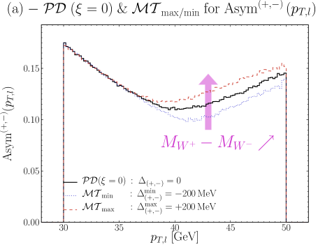
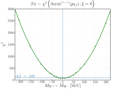
(c) Double charge asymmetry method
The event samples for this methods are exactly the same as for the charge asymmetry method. The event samples have been simulated in two steps corresponding to the two half-a-year periods of data taking corresponding to the two magnetic field configurations.
6.2.3 Scaling distributions for quarks flavors systematics
Most of systematic measurement and modeling biases discussed in this work lead to a distortion of the distributions and do not change their overall normalisation. The notable exception, discussed in more detail in the next section, are the biases driven by the PDFs uncertainties. These biases cannot be “absorbed” by the corresponding shifts and require an adjustment of the event/nb normalisation of the corresponding samples to obtain acceptable values.
The most natural method would be to extend the one-dimensional analysis presented in this section into two-dimensional analysis of both the mass and the normalisation parameters. Such an analysis would have, however, “squared” the necessary computing time of the samples and, therefore, was not feasible in our time-scale. Instead, we have tried to un-correlate the adjustment of the normalisation parameter and the mass parameters. As can be seen in Fig. 6.4.(a) the distribution is, in the region of small (), independent of the variations of over the range discussed here. We use this observation and modify correspondingly the likelihood analysis method. Before calculating , the and distributions are integrated in the range :
| (6.16) |
giving respectively two scalars : and . Then we re-normalise the distribution by the factor and calculate the values for the rescaled distributions. We have checked that the above procedure improves significantly the resulting values for each of the three analysis methods. By changing the integration region we have verified that the above procedure does not introduce significant biases in the estimated values.
The effect of this trick can be visualised on a concrete example where we consider the incriminated bias to reflect an overestimation of the PDF. The consequences of the different cross section between the with respect to the one of the central () histogram can be seen directly in Fig. 6.5.(a) and more finely in frame (c) where the normalised difference between the two histograms have been drawn. In (c) then, we observe an overall scaling factor –constant below the jacobian peak– between the two plots that will ultimately wreck any chance for the test to converge and then give a relevant result. Computing the scalars and allows to scale by multiplying it with as shown in Figs. 6.5.(b) and (d).
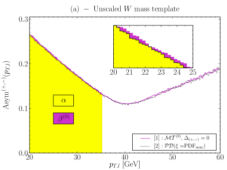
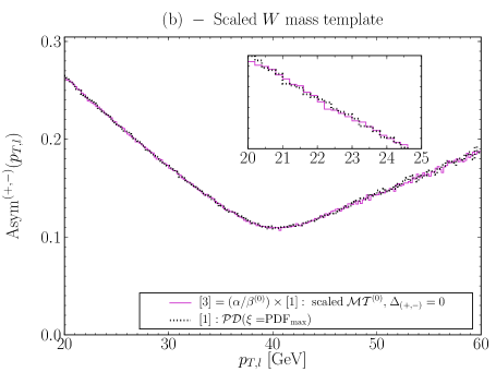
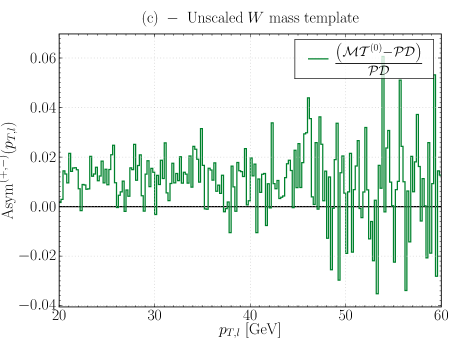
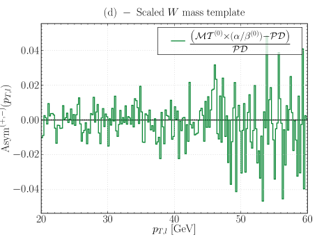
6.3 Systematic error sources
In this section we identify and model the systematic error sources that will limit the precision of the measurement at the LHC. Each of these error source will be modeled and reflected in the corresponding sample of events.
These error sources are of two kinds : (1) those reflecting uncertainties in modeling of the boson production and decay processes, (2) those reflecting the event selection and event reconstruction biases. A large fraction of the error sources have been identified [51] and reevaluated in the context of the measurement of the average mass of the boson at the LHC [57, 58]. We focus our discussion on the dominant errors for the measurement of the mass charge asymmetry, in particular on those that are specific to the LHC environment and have not been identified in the earlier studies. We shall not discuss here : (1) the measurement errors reflecting the uncertainties in the background estimation and in the efficiency of the events selection, (2) other measurement uncertainties which can be studied to the required level of precision only once the real data are collected. As demonstrated in the analysis of the Tevatron data [51], they are of secondary importance.
6.3.1 Phenomenological modeling uncertainties
The uncertainties in the modeling of the production and decay of the bosons include : (1) the uncertainties in modeling of non-perturbative effects, (2) the approximations present in theoretical modeling of the perturbative EW and QCD effects, (3) the uncertainties in the parameters of the Standard Model and (4) a possible presence of the Beyond Standard Model (BSM) effects, affecting both the production and decay mechanisms of the bosons. The two first items of them limit our present understanding of the Wide-Band-partonic-Beam (WBpB) at the LHC.
(a) WBpB at LHC
The measurement precision of the mass charge asymmetry will depend upon the level of understanding of the flavour structure, the momentum spectrum and the emittance of the WBpB at the LHC collision energy. The hard scale dependent emittance of the WBpB is defined here, in analogy to the emittance of the parent hadron beam, in terms of its transverse momentum distribution and in terms of its transverse and longitudinal beam-spot sizes. The above dynamic properties of the WBpB are highly correlated. Only their scale dependence can be controlled by the Standard Model perturbative methods. In addition, several aspects of such a control, in particular the precise modeling of the correlations between the flavour, the longitudinal and the transverse momentum degrees of freedom of the WBpB have not so far been implemented in the Monte Carlo generators available for the initial phase of the LHC experimental program.
The statu quo of understanding of the WBpB at the LHC is driven by the presently available Monte Carlo generator tools. Within this statu quo, the flavour dependent longitudinal momentum distribution of the WBpB, specified by ‘collinear’ PDFs, is fed to one of the available parton shower MC generators. The transverse momentum distribution of the WBpB is then derived from the assumed longitudinal one. This procedure depends upon a particular evolution scheme dependent form of the parton shower and upon the order of the perturbative expansion. It depends as well upon the modeling method of the quark flavour (quark mass) effects in the parton shower generation. The effects of the flavour dependence of the beam size in the transverse plane are partially controlled using auxiliary, impact parameter dependent re-summation procedures. Finally, the scale dependent evolution of the longitudinal beam spot size is presently assumed to be driven by the DGLAP evolution equations [30, 31, 32].
It is obvious that the precision of the present understanding of the WBpB at the LHC is difficult to asses within the above modeling environment. Since its impact on the precision measurements of electroweak processes will be significantly higher for the LHC WBpB with respect to the Tevatron one, some novel measurement and/or modeling schemes must be developed. They must assure either better theoretical control of the WBpB parameters or, as proposed, reduce their impact on the measured observables to such an extent that their detailed modeling becomes irrelevant. For the latter strategy it is sufficient to rely on crude modeling methods of the WBpB at the LHC which are available within the WINHAC generator.
(b) Uncertainty of PDFs
The uncertainties in PDFs are, most often, propagated to the measurement errors of the physics observables by varying the PDF sets chosen in the event generation process. Alternatively, the uncertainties of the QCD fit parameters of a given PDF set are propagated by re-weighting the generated events with “min” and “max” weights, , where are the central value distributions of a given PDF set and is computed according to the method described in Ref. [66]. We followed the latter method, mostly because of computing time constraints. We have used the CTEQ6.1M PDF set [192] in modeling of the standard PDFs uncertainties. The above methods, in our view, largely underestimate the influence of the PDFs uncertainty on the measurement precision of the boson mass.
As discussed in the last Chapter, the charge asymmetry of the boson production and decay processes is sensitive : (1) the presence of valence quarks in the WBpB, (2) the flavour asymmetry of their longitudinal momentum distribution (called hereafter the asymmetry) and (3) the asymmetry in the relative momentum distribution of the strange and charm quarks (the asymmetry). The corresponding uncertainties must be modeled directly using the existing (future) experimental constraints rather than be derived from the uncertainty of the PDF set parameters. This is because they are driven almost entirely by the non perturbative effects, and because the QCD evolution effects are, except for the quark mass dependency, flavour independent.
(c) Uncertainty of asymmetry.
We assume the following two ways of modeling the uncertainty in the asymmetry :
| (6.17) |
and
| (6.18) |
The first one preserves the sum of the distribution of the and quarks and is constrained, to a good precision, by the measured singlet structure function in neutrino and anti-neutrino Deep Inelastic Scattering (DIS) of isoscalar nuclei. At the LHC the sum of the distributions will be constrained by the rapidity distribution of the bosons ( quarks and quarks contribute with similar weights). The second one assures the correct propagation of the measurement errors of the sum of the charge square weighted distributions of the and quarks, constrained by the high precision charged lepton beam DIS data, to the uncertainty of the individual distributions.
While the sums of the distributions are well controlled by the existing and future data, their mutually compensating shifts are not. The only experimental constraints on such shifts come from : (1) the measurements of the ratio of the cross sections for deep inelastic scattering of charged leptons on proton and deuteron targets and (2) the measurements of the ratio of the neutrino–proton to anti-neutrino–proton DIS cross sections. They determine the present uncertainty range of the asymmetry. Improving this uncertainty range in the standard LHC colliding mode will be difficult and ambiguous. It will require simultaneous unfolding of the momentum distribution and the charge asymmetry of the sea quarks.
(d) Uncertainty of asymmetry
The annihilation represent of the total contribution to the boson production cross section at the Tevatron collision energy. At the LHC collision energy it rises to and becomes charge asymmetric : for the boson and for the boson. The uncertainty in the relative distribution of the strange and charm quarks becomes an important source of systematic measurement errors of both the average boson mass and its charge asymmetry.
We assume the two following ways of modeling the uncertainty in the asymmetry :
| (6.19) |
with representing respectively the present and future uncertainty range for the relative shifts in the and quark distributions. As in the case of the asymmetry, we have assumed that the sum of the distribution of the and quarks will be controlled to a very good precision by the boson rapidity distribution. Therefore we have introduced only unconstrained, mutually compensating modifications of the and quark distributions111In reality, the and quarks couple to the boson with slightly different strength but the resulting effect will play no important role in the presented analysis.. As seen previously in Eqs. (5.2) and (5.3), the valence quarks excess magnifies the contribution of the uncertainty to the measurement precision of boson mass.
(e) WBpB emittance
The and longitudinal momentum asymmetries would have no effect on the measured boson mass asymmetry in the case of the collinear partonic beams. The angular divergence (transverse momentum smearing) of the WBpB at the LHC is driven by the gluon radiation. Its parton shower Monte Carlo model determines the relationship between the longitudinal and the transverse degrees of freedom of the WBpB. It gives rise to the parton shower model dependent asymmetries of the and boson transverse momenta.
Instead of trying to estimate the uncertainties related to the precision of the parton shower modeling of the the quark flavour dependent effects, we allow for exceedingly large uncertainty in the size of the flavour independent primordial transverse momentum Gaussian smearing of the WBpB : (the samples have been simulated for the following values of the sigma parameter of the Gaussian smearing : ). Such a large uncertainty range, easily controllable using the boson transverse momentum distribution, represents the effect of amplifying (small values of ) or smearing out (large values of ) the flavour dependent asymmetries of the WBpB transverse momentum. The range has been chosen to be large enough to cover the uncertainties due to : (1) non perturbative effects, e.g. those discussed in [193], (2) the quark mass effects and (3) re-summation effects.
(f) EW radiative corrections
Out of the full set of the EW radiative corrections implemented in the WINHAC generator, those representing the emission of real photons could contribute to the measured mass charge asymmetry. Two effects need to be evaluated : the charge asymmetric interference terms between the photon emission in the initial and final states, and the radiation of the photons in the boson decays in the presence of the couplings. The above corrections are described to a high precision by WINHAC, as has been shown in Refs. [140, 142]. Therefore, their influence on the mass charge asymmetry measurement can be modeled very accurately. We did not considered these effects, leaving a detailed study for our future works.
6.3.2 Experimental uncertainties
(a) Energy scale (ES) of the charged lepton
The uncertainty in the lepton energy scale is the most important source of the measurement error for the Tevatron experiments. At the LHC, the production of unequal numbers of and bosons, its impact on the overall measurement precision will be amplified. For the measurement methods discussed the lepton energy scale error will be determined : (1) by the curvature radius measurement errors, (2) by the uncertainties in the magnetic field maps within the tracker volume and (3) by the modeling precision of the physics processes which drive the link between the measurements of the particle hits in the tracker and the reconstructed particle momentum. While the first two sources of the measurement error are independent of the lepton flavour, the third one affects the electron and muon samples differently. In the following we shall assume, on the basis of the Tevatron experience, that modeling of physics processes of particle tracking will be understood at the LHC to the required level of precision, on the basis of dedicated auxiliary measurements222For example, the energy loss of the electrons in the dead material within the tracker volume will be understood using a conjugate process of the photon conversion.. This simplification allows us to discuss the muon and electron track measurement simultaneously. We assume as well that the solenoid magnetic field strength in the volume of the tracker will be understood to better than of its nominal value. We base this assumption on the precision of achieved e.g. by the H1 experiment at HERA [194] and by the ALEPH experiment at LEP [195]. If this condition is fulfilled, the energy scale error is driven by the curvature radius measurement error
| (6.20) |
where and are, respectively, the reconstructed and the true curvature smeared by the unbiased detector response function.
Based on the initial geometrical surveys, the initial scale of will be known to the precision of . This precision will have to be improved at least by a factor of 10 to match the precision of the Tevatron experiments, if the same measurement strategy is applied. To achieve such a precision, the local alignment of the tracker elements and/or average biases of the reconstruction of the trackers space-points must be known to the precision. In addition, the global deformation of the tracker elements assembly must be controlled to a precision which is beyond the reach of the survey methods.
Several modes of the global deformations can be considered in a first approximation as discussed in Ref. [107]. Below we make a sum up of the conclusions drew from § 3.4 and Appendix 3.A. The main difference between the measurements of the boson properties at the Tevatron and the LHC boils down to their sensitivity to the different types of the global deformation modes. Both for the Tevatron and LHC measurements the translations are of no consequences since they do not affect the shape of the transverse projection of the particle helix. The deformations (the radial expansion , the elliptical flattening and the bowing ) give rise to common biases for positive and negative particle tracks. On the other hand, the curl and twist deformations give rise to biases which are opposite for negative and positive particles. In the case of the Tevatron collisions, producing equal numbers of the and bosons, the dominant effect of -coherent curling of the outer tracker layers with respect to the inner tracker layers has residual influence on the uncertainty of the average boson mass, leaving the residual effect of relative twist of the and sides of the tracker volume as the principal source of the measurement error. For the LHC collisions, producing unequal numbers of the and bosons, both deformation modes influence the measurement biases of the average boson mass. In the case of the LHC there is no escape from the necessity of precise understanding of the lepton charge dependent biases on top of the lepton charge independent biases.
In the presence of the above two sources of biases the energy scale bias can be expressed in the limit of small deformations (cf. Eqs. (3.22–3.23)) as follow
| (6.21) | |||||
| (6.22) |
where represents the particle charge dependent -type bias and represents the charge independent -type bias.
While the -type biases can be controlled with the help of the boson, and “standard candles”, e.g. using the CDF procedures, the global charge dependent and symmetric biases cannot. At the Tevatron these biases were investigated using the electron samples by studying the charge dependent distribution, where is the energy of the electron (positron) measured in the calorimeter and is its reconstructed momentum. The relative scale error of positive and negative electrons was re-calibrated using the mean values of the distributions. The achieved precision was the principal limiting factor of the measurement of . Even if the statistical precision of such a procedure can be improved significantly at the LHC, this method is no longer unbiased. This is related to the initial asymmetry of the transverse momentum distribution for positive and negative leptons in the selected boson decay samples. As a consequence, both the positive and negative lepton events, chosen for the calibration on the basis of the energy deposited in the calorimeter, will no longer represent charge unbiased samples of tracks. The biases will be driven both by the influence of distribution shape and by the migration in and out of the chosen energy range. A partial remedy consists of using a statistically less precise sample of positive and negative lepton tracks in a selected sample of boson decays. However, due to the different weights of the and couplings of the boson to leptons, even these track samples are biased. In both cases these biases can be corrected for, but the correction factor will be sensitive to the uncertainty in the momentum spectra of the valence quarks.
Given the above sources of the uncertainties, we assume the following two values for the size of the biases, both for the charge independent and charge dependent scale shifts
| (6.23) | |||||
| (6.24) |
The first value corresponds to the precision which can be achieved on the basis of the initial geometrical survey and the initial measurement of the field maps. The second one corresponds to what, in our view, can be achieved using the above data based on the calibration methods –given all the LHC specific effects– which make this procedure more difficult at the LHC than at the Tevatron.
(b) Resolution (RF) of the charged lepton track parameters
The finite resolution of measuring the lepton track parameters may lead to biases in the measured value of . We model the possible biases introduced by the ambiguity in the assumed size of the (Eq. (3.15)) and (Eq. (3.16)) smearing by decreasing or increasing the widths of their Gaussian distributions by the factor .
6.4 In search for the optimal measurement strategy
6.4.1 Validation of the framework and behaviour of the likelihood analysis
Before presenting the results, now that we have a global idea of the challenge we present a few more details on the validation of the analysis framework from both technical and physical point of views and look also at the influence on the results of some input parameters to the analysis process. The following tests were performed for trivial () as well as non trivial results () when necessary, i.e. when and/or . Since most of these tests are quite redundant they were not included in the core of the Chapter in the aim not to break the flow of the expose. Rather than that, the gist of it was compiled at the end of the present Chapter. Hence, in what follows the corresponding sections in the Appendix are indicated so that the reader wishing to have quantitative results on a particular topic knows where to find them.
The first test consisted to cross check the framework using for all three methods the observable (§ 6.A.1.(a)). All results ( and ) confirmed the calculus using -based methods.
Since trivial validation tests () displays the relevancy of the sign of the result cannot be checked, also we generated with a shift of with respect to the mass of reference of the bosons and saw that indeed the signs were coherent (§ 6.A.1.(b)).
Using these shifted masses in the allow on a technical level to see at which level the convergence of a result depends of the number and localisation of from the minimum of the parabola. Thus, by playing with the number of the samples participating to the analysis and choosing them such that all masses are far and on one side only from the minimum we can show that the convergence, and in consequence , suffers in such extreme configurations (§ 6.A.2.(a)). Nonetheless the order of the size of the error is respected. Also, despite our reduced number of samples, in what follows results displaying large values of can be trusted.
The influence of the detector resolution on the results was investigated by increasing the size of the bin widths of the and histograms before performing the analysis. It proved that the test is quite robust so that values are very close to the one obtained with the nominal resolution, excepted for the convergence accuracy which suffers much more from lower resolution when (§ 6.A.2.(b)).
The charge asymmetry method being new we considered a spread in the analysis range to perform the analysis which is not possible in the classic method without a very good knowledge of the background at low and of the influence of at high . Tests based on performed in the range and then in displayed no real enhancements on the results apart from slightly increasing the precision of the convergence (§ 6.A.2.(c)). This can be understood as the mass of the has a real impact on the region where the jacobian peak arise. Nonetheless with real data this could provide a good test to see a dependence of the results from the background and width influence on the extraction of the mass with this method.
Last but not least the test of the influence of a cut on the result was performed by doing at the stage of the generation directly a cut on . The consequences on the results are absolutely not visible and it is believed that a realistic cut based on would display the same feature (§ 6.A.2.(d)). This test justify then the non treatment of realistic cuts and recoil modeling in our analysis.
To conclude, from all these tests the one having the most striking effect on the calculus was found to be the lack of samples thinly separated and covering a large range of masses. As stated previously the CPU was prohibitive to refine the analysis and would not have brought much enhancement as most of the systematic error absolute values, as it will be shown, are such that . Also, to preserve a better clarity of the discussion –as independent as possible from the choice of the input parameters– we have chosen that all the presented in the core of the Chapter were made for mass templates covering the range .
Finally, just out of curiosity and to insist on the difference between the kinematics of the charged lepton decaying from a or a at the LHC we considered the case where –not aware of the coupling of fermions in electroweak interactions– the test is made between pseudo-data related to the information and the mass templates related to the information. Performing such a naive test assuming similar kinematics for the positive and negative charged leptons gives absolutely non relevant results, such that and (cf. Appendix 6.B).
6.4.2 Reducing impact of systematic measurement errors
In Section 6.1 three measurement methods of have been presented : the classic, charge asymmetry and double charge asymmetry methods. The basic merits of the two latter methods is that they use the dedicated observables which are meant to be largely insensitive to the precise understanding of the event selection and reconstruction efficiency, the background contamination level, understanding to the absolute calibration and the biases of the reconstruction of the neutrino transverse momentum, the internal and external (dead-material) radiation. It will remain to be proved, using the data collected at the LHC, that all these error sources have negligible impact on the precision of the measurement. At present, such a statement must rely on the extrapolation of the Tevatron experience. In what follows, links to detailed comments and/or graphics for each addressed systematic error are made to the Appendix 6.C since for clarity we kept only the essential information in the core of the Chapter.
The impact of the remaining measurement errors specified in the previous Section and quantified using the analysis methods discussed in Section 6.2 is presented in Table 6.4.
The precision of estimating the systematic shifts of for each of the systematic effect and each measurement method is assessed using the validation procedures described in Section 6.2. The resulting of corresponds the collected luminosity of . The first observation is that the precise understanding of the measurement smearing RF of the track parameters does not introduce any bias in the measured values of . The impact of the energy scale errors on the biases differs for each of the discussed methods.
| Systematic | “Classic” Method | |||||
| MC truth | ||||||
| Cent. Exp. | ||||||
| ES [%] | ||||||
| 1 | ||||||
| -1 | ||||||
| RF | ||||||
For the lepton charge independent shift even the “initial” () scale error has no statistically significant impact on the measurement precision for the charge asymmetry method. For the classic method the scale error has to be reduced to the “ultimate” value of () to achieve a comparable measurement precision of .
For the lepton charge dependent shifts the classic and asymmetry methods provide similar measurement precision. The measurement error remains to be of the order of even if the ultimate precision of controlling the energy scale biases to is reached. The double charge asymmetry method reduces the measurement error to the extend that the resulting bias is statistically insignificant, even for the initial scale uncertainty. This is illustrated in Figures 6.6.(a) and 6.6.(b). These plots show the comparison of the fits for the charge asymmetry method and the double charge asymmetry method for the lepton charge dependent scale error of (a), and the fit corresponding to for the double charge asymmetry method (b). The results for the double charge asymmetry correspond to for the first running period with the standard magnetic field configuration and for the running period with the inverted direction of the -component of the magnetic field.
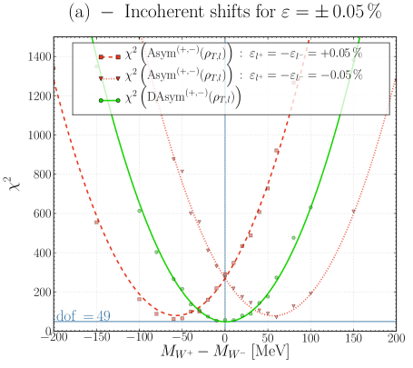
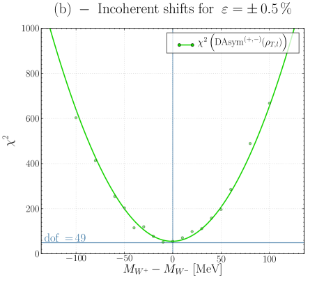
The above reduction of the measurement sensitivity to the energy scale error can be achieved for the initial survey precision of the tracker alignment. Such a survey will have to be made at the beginning of each of the two running periods. A special care will have to be taken to understand the relative curl and twist deformations induced by reversing the current in the solenoid. It has to be stressed that the precision of the double charge asymmetry method is insensitive to the relative biases of the reconstructed hit positions for the two data taking periods, provided that they are not larger than times the average hit reconstruction precision achieved in the standard field configuration running period. Worsening of the hit position resolution for the inverted field configuration, driven by the geometrical layout of the silicon tracker modules, have no significant effect on the measurement precision. Similarly, the required level of precision of understanding the hysteresis effects, leading to inequality of the absolute field strength in the two running periods, corresponding to reverse solenoid current directions can be achieved with the standard field mapping methods. Note that the precision required for the asymmetry measurement may be up to times worse with respect to the one needed for the measurement of the average boson mass. The reduced sensitivity to all the above effects is due to the fact that the impact of each of these effects is, to a large extent, canceled in each of the running periods. This is done in the same way as canceling the time-dependent effects of the detector response, calibration and alignment procedures. Note, that the residual impact of all the above effects can be reduced further (if necessary) using the -field configuration dependent analyses of straight track residua and/or the position of the reconstructed boson mass peak.
6.4.3 Reducing impact of systematic modeling errors
As discussed in the previous section, by using the charge asymmetry (double charge asymmetry) methods the systematic measurement precision of could be reduced to the level of . In this section we discuss the impact of the modeling uncertainties described in Subsection 6.3.1 on the measurement precision of for the charge asymmetry method333From the point of view of the modeling uncertainties, the charge asymmetry and the double charge asymmetry methods are equivalent and the discussed results are the same for both methods.. The detailed discussion and graphics related to the systematic errors due to the uncertainties on the intrinsic , global PDF, the valence and sea asymmetry are present from § (c) through § (e) of Appendix 6.C.
In Table 6.5 we show, in the first column, the expected measurement biases of due to the dominant modeling uncertainties, discussed in the previous section, for collisions at the LHC energy. We do not see a significant impact of the coherent shifts of the partonic distributions, defined in the previous section and denoted as the PDFs uncertainty. It would be, however, misleading to conclude prematurely that the biases are insensitive to the uncertainties in the partonic distributions.
| results using the Charge Asymmetry of | |||||||||
| Systematic | - | - | - | - | |||||
| MC truth | |||||||||
| Cent. Exp. | |||||||||
| [GeV] | |||||||||
| PDF(∗) | Min. | ||||||||
| Max. | |||||||||
Indeed, the present uncertainty of the relative distribution of the the and valence quarks (the asymmetry) leads to large shifts in the values. These shifts are specific to the LHC collider and are largely irrelevant for the Tevatron collisions. This might explain why they were neglected in the previous studies [57, 58], in spite that they concern the average boson mass measurement. There are three origins for these shifts. The effects due to each of them add up and result in the amplification of the biases. The discussion and the numbers provided in § 5.A.6 of Chapter 5 might be helpful to understand the following ideas. Firstly, increasing the content of the proton shifts downwards the average momentum of the anti-quarks. This leads to an increase of the average transverse momentum of the anti-quarks producing , mimicking the increase of the boson mass. Simultaneous decreasing of the acts in the opposite direction for , i.e. this time the average of the colliding sea quark decreases which lead to large and positive values of . Secondly, at the LHC, contrary to the Tevatron, the presence of the quarks leads to an asymmetry in the production rate of the boson from the quarks and anti-quarks. Since the average transverse momentum of the charm quarks is higher with respect to the light quarks, this asymmetry shows up in the relative shifts in the distributions for positive and negative leptons. Increasing the density of the quarks mimics thus the effect of increasing the mass of the with respect to the boson. The above two effects are amplified by the bias in the degree of the transverse polarisation of with respect to , induced by the event selection procedure based on the lepton kinematics. The relative movements of the and amplify (attenuate) the initial event selection procedure bias. What must be stressed is that if the shifts are compensated by the corresponding shifts of the distributions, they cannot be constrained to a better precision by the present data, and they will not affect the rapidity distributions of the boson. Thus, it will be difficult to pin them down using the standard measurement procedures.
The uncertainties of the relative density of the strange and charm quarks, the asymmetry, gives rise to smaller but significant biases in the values, as shown in the first column of Table 6.5. Since the transverse momentum of the quarks is significantly higher than the corresponding momentum for the quarks, this effect, even if Cabbibo suppressed, cannot be neglected. What must be stressed again is that if the shifts are compensated by the corresponding shifts of the distributions, they will not affect the rapidity distributions of the bosons. Thus, it will be difficult to pin them down using the standard measurement procedures. This asymmetry can be constrained unambiguously only by using dedicated measurements, e.g. by measuring the associated production of the bosons and charmed hadrons.
Compared to the above, the biases corresponding to the uncertainties in the flavour independent smearing of the intrinsic transverse momentum distribution of partons are smaller in magnitude and can be neglected, if the intrinsic transverse momentum of partons is controlled to the precision of .
It is obvious from the above discussion that using the standard measurement procedures, the modeling uncertainties will be the dominant source of the measurement errors of the boson mass asymmetry, already for the collected luminosity times smaller than the one considered here. In order to diminish the impact of the modeling errors on the measurement of to a level comparable to statistical and experimental measurement errors, some dedicated measurement methods must be applied. Two such procedures are proposed and evaluated below : (1) the narrow bin method and (2) the isoscalar beams method.
(a) Narrow bin method
As discussed previously, the dominant source of large uncertainties in comes from the presence of the valence quarks in the WBpB and from the uncertainties in their flavour dependent momentum distributions. In order to reduce this effect we propose to profit from the large centre of mass energy of the LHC and measure using a selected fraction of the bosons which are produced predominantly by the sea rather than by the valence quarks. These bosons are produced with small longitudinal momentum in the laboratory frame.
Two methods of selecting such a sample are discussed below. The first is based on restricting the measurement region to . The merit of the -cut based selection is that it uses a directly measurable kinematic variable. Its drawback is that rather broad spectrum of the longitudinal momenta of annihilating partons is accepted due to the large mass of the boson. The second is based on restricting the measurement region to . Here, only a narrow bin of the longitudinal momenta of annihilating partons is accepted in the region where the sea quarks outnumber the valence quarks. However, cannot be measured directly. It has to be unfolded from the measured transverse momentum of the charged lepton and the reconstructed transverse momentum of the neutrino. The unfolding procedure [67] neglects the width of the boson and depends upon the initial assumption of the relative momentum spectra of the valence and sea quarks. However, in the selected kinematic region the above approximation are expected to lead to a negligible measurement bias. It has to be stressed that the narrow bin measurements will require a times higher luminosity to keep the statistical error of at the level of . Therefore, the results presented below for the narrow bin method correspond to an integrated luminosity of and are based on the dedicated set of the simulated mass template and pseudo-data samples. Each sample contains and simulated (weighted) events, respectively.
The systematic biases of due to modeling uncertainties discussed in the previous sections are presented in columns 2 and 3 of Table 6.5 respectively for the and selections. The -cut based method reduces slightly the biases related to the uncertainties in the and asymmetries. The gain in the measurement precision is clearly seen for the -cut based method which reduces to a negligible level the biases. It is interesting to note that the shifts in change their signs for the above two methods, reflecting the importance of the boson polarisation effects discussed earlier.
The narrow bin method allows, thus to reduce the impact of the boson modeling uncertainties on the biases to the level comparable to the statistical precision for all the effects, except for the asymmetry effect. Here another remedy has to be found.
(b) Isoscalar beams
Isoscalar targets have been successfully used in most of the previous fix-target deep inelastic scattering experiments at SLAC, FNAL and CERN, but this aspect has been rarely discussed in the context of the electroweak physics at the LHC. The merits of the ion beams for the generic searches of the electroweak symmetry breaking mechanism at the LHC have been discussed in [144]. Their use as carriers of the parasitic electron beam, to measure the emittance of the WBpB at the LHC, has been proposed in [196]. In our work we strongly advocate the merits of the isoscalar beams in improving the measurement precision of the parameters of the Standard Model. In this section we discuss their role in increasing the precision of the measurement of . We shall consider light ions : deuterium or helium. As far as the studies of the boson asymmetries are concerned, they are equivalent because shadowing corrections are quark-flavour independent. The energies of the LHC ion beams satisfy the equal magnetic rigidity condition. For the isoscalar beams the nucleon energy is thus two times lower that the energy of the proton beam. In the presented studies we assume that the ion–ion luminosity is reduced by the factor with respect to the luminosity (cf. § 3.1.1).
In column 4 of Table 6.5 we present the impact of the modeling uncertainties on the biases. The isoscalar beams allow to reduce the measurement biases due to the asymmetry effect to a negligible level. This colliding beam configuration allows to profit from the isospin symmetry of the strong interactions which cancels the relative biases in the momentum distribution of the and quarks. It is interesting to note that, as expected, the biases are similar for the proton and for the light isoscalar beams. On the contrary, the biases related to the flavour independent intrinsic momentum of the quarks and anti-quarks are amplified due to the reduced centre of mass collision energy444In order to amplify this effect, we have kept the same central value of the intrinsic transverse momentum smearing in the reduced collision energy as for the nominal collision energy.. Indeed, as seen already in § 5.A.7 we came up to the conclusion that at lower energies in the center of mass the charge asymmetry in the final state is much more visible since the charge symmetric sea contributions are not large enough.
6.4.4 Two complementary strategies
Two complementary strategies to achieve the ultimate measurement precision of will certainly be tried. The first one will be based on an attempt to reduce the size of the systematic measurement and modeling uncertainties, discussed in the previous section. In our view, such a strategy will quickly reach the precision brick wall – mostly due to the a lack of data-driven constraints on modeling the flavour dependent boson production at the LHC energy. The second one, instead of reducing the size of the uncertainties, attempts to reduce their impact on the systematic error of the measured quantity by applying the dedicated methods. Such a strategy requires running the dedicated machine and detector configurations. It is thus time and luminosity consuming. However, in our view, only such a strategy allows to measure the mass charge asymmetries at the precision comparable to the one achieved in the muon decay experiments.
Let us recollect the main elements of the proposed dedicated measurement strategy that allow to reduce the systematic errors to the level shown in the shaded areas of Table 6.5 :
-
-
The charge asymmetry method allows to reduce the impact of most of the systematic measurement errors, except for the relative momentum scale errors for the positive and negative leptons. If they cannot be experimentally controlled to the level of , their impact can be drastically reduced in the dedicated LHC running periods using the double charge asymmetry method.
-
-
The impact of the uncertainty in modeling of the intrinsic transverse momentum of the WBpB can be reduced to a negligible level using the narrow bin measurement method.
-
-
The impact of the uncertainty can be attenuated using the selection based method in narrow bin.
-
-
Finally, the impact of the uncertainty can be annihilated in the dedicated LHC runs with light isoscalar beams.
Appendix 6.A Validation tests and miscellanea technical variations of the analysis
Buster : “Actually, I’m studying cartography now, the mapping of uncharted territories.”
Michael : “Sure. Hasn’t everything already sort of been discovered, though, by, like Magellan and Cortés? NASA,…you know ?”
Buster : “Oh, yeah, yeah…Those guys did a pretty great job.”
Lucile : (appearing between her sons) “Never hurts to double-check.”Arrested Development - Extended Pilot
This Appendix presents in details the validations tests that were achieved to improve the analysis framework. The points addressed are the following.
The first part presents trivial results carried using the observable to crosscheck the one made with . Other trivial tests were made as well with -based distributions using shifted masses in the pseudo-data. The second part treats of the steadiness of the results with respect to certain input parameters for the analysis, such as the influence of the number of templates and their localisation with respect to the minimum, the number of bins of the histograms, the window range for the analysis and the emulation of cuts.
In the rest of this Appendix unless stated otherwise the tests are made preferentially using collisions selected with the requirements shown in Eq. (6.6) and in the conventional range of .
6.A.1 Details on the validation of the analysis framework
(a) Cross check of the analysis using the observable
Since the observable is booked at the time of the generation it is pertinent to cross check the framework with -based methods for the case of trivial () as well as non trivial () tests. Besides, this simple studies allows as well to get accustomed to the behaviour of the variable and . Starting with that last remark, Figure. 6.7 presents in frames (a), (b) the behaviour of the observable for : (1) the generated and unselected sample of events, (2) the generated and selected sample of events and (3) the unbiased simulated detector response and selected sample of events. In the each frame the range for the analysis –equivalent to – is highlighted. Just like for the distribution we can see that the cuts are responsible of a drastic change in the behaviour of the spectrum in particular in the region of the jacobian slope. In Fig. 6.7.(d) a trivial test was performed for an unbiased pseudo-data using . As expected the value is found. The results for were found to be in a complete agreement –up to non avoidable numerical discrepancies– with the one provided by -methods.
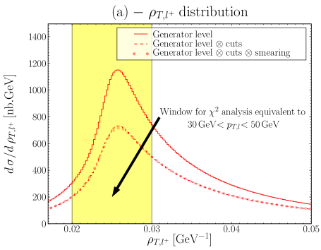
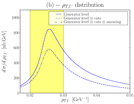
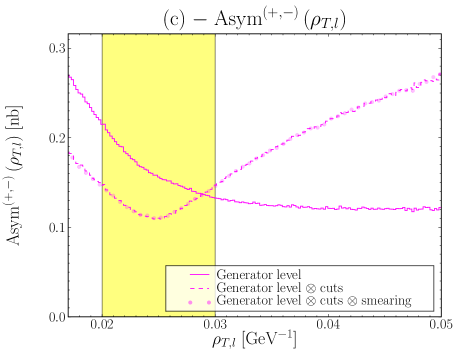
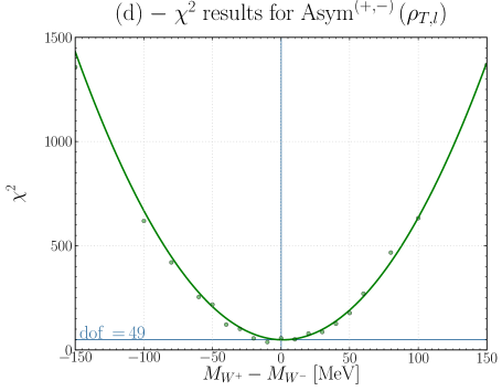
(b) Validation using shifted mass for the W boson mass in the pseudo-data
Even though the previous trivial tests were found to be relevant, as long as the value doesn’t have a sign it is –so far– impossible to fully check the relevancy of the values. Also, the next logical step was to simulate unbiased pseudo-data but with shifted masses with respect to for the boson and see if in the analysis we rediscover those shifts. Three tests were carried for that purpose using both classic and charge asymmetry methods. In each of these tests, the central values for the masses of the and bosons were fixed for the generation of the pseudo-data to :
-
1.
.
-
2.
.
-
3.
.
while the remained the same i.e. generated with no biases and with and where for reminder .
The Figure 6.8 presents in the first three frames ((a), (b) and (c)) the histograms of , and for the case (1) of the previous item list where the mass of the has been fixed to while the mass of the has been kept to . The two extrema samples, and , have been drawn as well to enhance the deviation of the unbiased with respect to the half way position between them. Starting with Fig. 6.8.(a), the jacobian peak of the is slightly shifted to higher while the one for in frame (b) is half-way between the two . In frame (c), the charge asymmetry of is closer to the for which . This is understandable as in general beyond the jacobian peak (i.e. or in -space) the following equation holds
| (6.25) |
where is to be replaced by or . Then, because of the form of the charge asymmetry (Eq. (2.13)), in this first test, increasing the mass increases the spectrum for each fixed value beyond the jacobian peak with respect to its former value eventually leading to an increase of both numerator and denominator. In the end, we observe that the kinematics at the LHC are such that the charge asymmetry of or are growing functions in the parameter as already hinted by the behaviour of the .
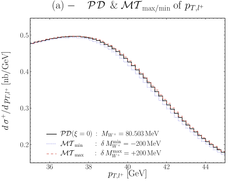
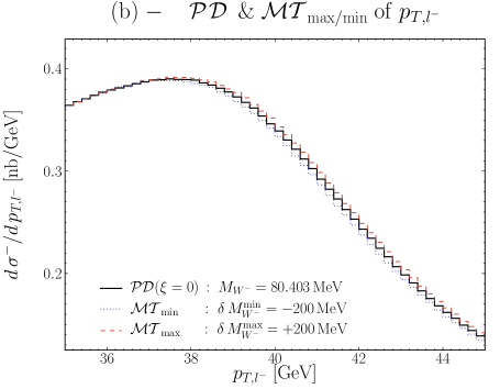
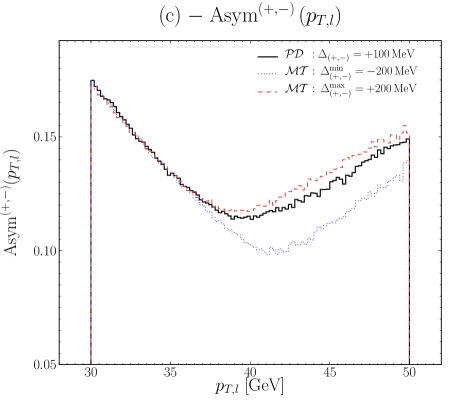
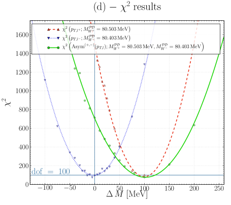
Finally the tests for the , and spectra are represented in Fig. 6.8.(d). The meaning of depends on the parabola we look at, we have :
| (6.26) | |||||
Starting with the associated to we find a shift of present in the pseudo-data with respect to the reference mass confirming that while looking at the negatively charged analysis we find . Finally the case of the analysis based on the charge asymmetry gives direct access to the charge difference between the masses of the pseudo-data bosons, that is . For the cases (2) and (3) of the previous item list the results where found to be relevant as well.
Let us note that in the case of the and parabola the fact there are less points in the vicinity of the parabola minimum does not decrease the degree of convergence of the calculus. For non trivial analysis where we often observe shifts of such amplitude that most of the points are localised on one side only of the fitted parabola. Hence a question we can ask is at which point the small number of considered mass templates is sufficient to provide a relevant value. In the next Subsection we investigate this issue by using the present pseudo-data for unbiased tests.
6.A.2 Influence on the results of some input parameters to the analysis
(a) Influence of the localisation and number of templates
In this part we consider the problem where the systematic error is such that there are no simulated mass templates having masses of the order of the systematic error. In other words we want to address the problem where we have to perform of parabola fit with the points being far from the parabola minimum and localised in one side only of the minimum. For that purpose we consider the same pseudo-data with than in the case (1) of the item list of the previous section, that is with , , and use the charge asymmetry method. This emulates in a good way the cases where for .
To sees at which point the localisation of the templates matters we reduce the range covered by the templates to see at which level the convergence and value changes. The results are shown in Table. 6.6.
| range [MeV] | [MeV] () | |
|---|---|---|
| 0.77 | ||
| 0.84 | ||
| 1.20 | ||
| 1.69 | ||
| 2.34 |
Then we come to the conclusion that as long as the systematic errors are such that if the convergence is poor () it has to be blamed purely on the distortion on the affected by the bias . On the other hand, for the cases where a bad convergence will always be observed because of the lack of mass templates which eventually will provide values of which will differ from the one to be observed if having generated much more templates.
Nonetheless, with the chosen biases values and the analysis techniques developed most of the errors are within the range which justify why the extension of the range was not considered a vital problem to extract the essential physics from our analysis.
(b) Influence of the resolution of the histograms
In this part we considered changes to larger bins for the analysis with respect to the one used for the generation to see at which level the bin width of the histograms is important. Let us remind the former binning corresponded to a resolution of , which in the range of corresponded to bins.
We present here the results for the classic and charge asymmetry methods in the case of collisions for the standard cuts of and . The likelihood test was carried for the case of unbiased pseudo-data (). The procedure for the likelihood test between the pseudo-data and the -mass template was done in two steps : (1) and histograms were re-binned to a lower resolution, (2) the likelihood analysis was carried out, i.e. the two histograms are cut to the standard analysis window of and then the test was done.
Table 6.7 shows the influence of different resolutions for the charged lepton on the results while Figure 6.9 present and spectra with a resolution of .
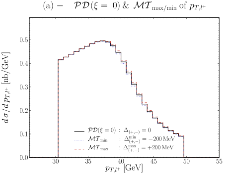
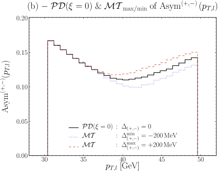
| Number of bins | [GeV] | Classic | Charge Asymmetry |
|---|---|---|---|
| 200 | 0.2 | ||
| 100 | 0.4 | ||
| 50 | 0.8 | ||
| 25 | 1.6 |
(c) Influence of the window in
We look now at the influence of the window for the analysis. Enlarging the range at low and high would imply in reality to test the sensibility of the charge asymmetry observable as a mean to extract the mass respectively toward the modeling of the low background differences between the and the production and the influence of the and/or in the high region.
In the first step the high is maintained at . Then, taking the minimum value of for the low cut we found for trivial results using the charge asymmetry of :
| (6.27) |
which does not enhance the former result seen in Eq. (6.15). Now, considering the whole range used for the and histograms, still using the charge asymmetry we find :
| (6.28) |
that is here we have a slightly better result.
Since the results do not change a lot this would eventually allow by first reducing the lower cut on to see the influence of the different background contributions in the positive and negative channels. Note that the lower cut should not be too close from the trigger cut to avoid the possible charge dependency from the selection process. On the other hand, maintaining the lower cut fixed and exploring higher cuts would allow now to study the influence of the boson width on the results.
(d) Influence of cuts
The influence of the cut was investigated with the best emulation achievable in our framework, that is during the generation process in top of the requirements from Eq. (6.6), the simulated events were selected if and only if the decaying neutrino displays . All ( and ), up to non avoidable numerical discrepancies, were of the same values than the data gathered without doing any cut on the neutrino.
Just to cite two numbers, the Monte Carlo truth test gave :
| (6.29) |
while the unbiased experimental test gave :
| (6.30) |
Both of these values are very close to the one present in Table 6.4. This justified for the rest of the study the non necessity to take care of such cuts.
Appendix 6.B Measurement of the W mass charge asymmetry : the How Not To
“That’s not right. It’s not even wrong.”
Wolfgang Pauli’s words of wisdom
(Kept alive nowadays by M.W.K.)
We consider a particular context to extract that stresses the charge asymmetry between the and distributions at the LHC. For that matter we propose to assume just for a moment that we are not aware of the coupling of bosons to fermions in the Standard Model and that the and , which are particle and antiparticle of each other provide positively and negatively decaying charged leptons with the same kinematics. Putting aside the fact that the detector measurement are different between positively and negatively charged leptons we consider the extraction of could be obtained directly by confronting the data from one charge to mass templates generated for the opposite charge.
To be more precise, the data is here represented by Monte Carlo pseudo-data simulations of the confronted via likelihood tests with Monte Carlo simulations of the bosons. Unaware of the coupling and of all its consequences seen in Chapter 5 one would expect that in this configuration a trivial test with unbiased pseudo-data should give with a good convergence ().
Figure 6.10 shows the test using the unbiased pseudo-data of the distribution and using for the mass templates (covering here the range ). The result obtained is and . The poor quality of this result can be understood using the arguments from the previous Appendix : the number of is too small and far from the expected parabola minimum. Nonetheless as we saw the order is still more or less correct and gives an idea of the size of the error, hence here we can say that going to such a naive test imply an error of the order of the which is completely ruled out by the actual measurements as seen in Table 2.2.
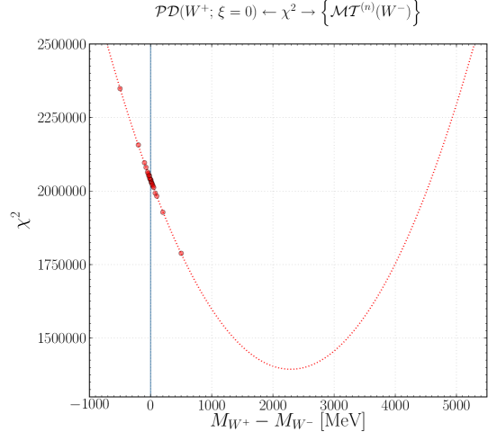
Appendix 6.C Step-by-step interpretations of systematic errors results
Reggie : “Trucks come in and out of here all day long. Truck comes in, you unload it. Truck goes out, you load it. Next truck comes in, you unload it. Next truck…”
Randy (very confused) : “Wait a second. Go back to that first truck.”My Name is Earl - Get a real job
In this Appendix more details are given on the results presented in the core of the Chapter. For that purpose step-by-step comments of the tables are provided with the help of visual support.
The first Subsection introduces the notation implemented in the more detailed versions of the tables shown in the core of the Chapter. Then in a second part the comments of these detailed tables are made based each time on the relevant and histograms and . The influence of the following effects are addressed in that chronological order
-
(a)
Energy scale of the charged lepton
-
-
Coherent biases between the positively and negatively charged lepton tracks (noted sometime for convenience “coherent biases”)
-
-
Incoherent biases between the positively and negatively charged lepton tracks (noted sometime for convenience “incoherent biases”)
-
-
-
(b)
Resolution of the charged lepton track parameters
-
(c)
Intrinsic of the partons
-
(d)
asymmetry
-
(e)
asymmetry
6.C.1 Detailed tables
The Tables 6.9 and 6.10 in the following pages are just reproduction of Tables 6.4 and 6.5 from the core of the Chapter with some additive information. More precisely, each systematic error is now given with a precision of along with the associated value providing then further details on the degree of convergence of the calculus.
Besides, as explained previously, different random numbers sets were used for each event generation to emulate as better as possible uncorrelated events. For that purpose independent seeds set were produced and tagged from set number to set number . Practically the generation of events needed to be achieved by splitting each generation into several sub-generations. Each sub-generation were produced so that all the seeds were different to ensure the best possible un-correlation between different event batches. For the standard generation of one year of low luminosity, each generation were split in average to sub-generations, hence we used here . Concerning the generation in the narrow lepton pseudo-rapidity or boson rapidity region this time each generation were split in average into hence here .
The seeds tags used for producing each pseudo-data will be as well displayed in the tables, the one for the being labeled “” each time written in top of the one used for labeled “”. Concerning the mass templates , each template seed tag are indicated on the next page in Table 6.8.
| [MeV] for | seed tag | seed tag |
|---|---|---|
| 0 | 10 | 50 |
| -5 | 11 | 51 |
| 5 | 12 | 52 |
| -10 | 13 | 53 |
| 10 | 14 | 54 |
| -15 | 15 | 55 |
| 15 | 16 | 56 |
| -20 | 17 | 57 |
| 20 | 18 | 58 |
| -25 | 19 | 59 |
| 25 | 20 | 60 |
| -30 | 21 | 61 |
| 30 | 22 | 62 |
| -40 | 23 | 63 |
| 40 | 24 | 64 |
| -50 | 25 | 65 |
| 50 | 26 | 66 |
| -75 | 27 | 67 |
| 75 | 28 | 68 |
| -100 | 29 | 69 |
| 100 | 30 | 70 |
| -200 | 31 | 71 |
| 200 | 32 | 72 |
| Systematic | Classic Method | ||||||
| MC truth | |||||||
| Cent. Exp. | |||||||
| ES [%] | . | . | |||||
| . | . | ||||||
| . | . | ||||||
| . | . | ||||||
| . | . | ||||||
| . | . | ||||||
| . | . | ||||||
| . | . | ||||||
| ERF | . | . | |||||
| . | . | ||||||
| Seed | using | |||||||||
| Systematic | - | - | - | - | ||||||
| MC truth | ||||||||||
| Cent. Exp. | ||||||||||
| [GeV] | . | . | . | . | ||||||
| . | . | . | . | |||||||
| . | . | . | . | |||||||
| . | . | . | . | |||||||
| . | . | . | . | |||||||
| PDF(∗) | Min. | . | . | . | . | |||||
| Max. | . | . | . | . | ||||||
| . | . | . | . | |||||||
| . | . | . | . | |||||||
| . | . | . | . | |||||||
| . | . | . | . | |||||||
| . | . | . | . | |||||||
| . | . | . | . | |||||||
| . | . | . | . | |||||||
| . | . | . | . | |||||||
6.C.2 Detailed comments and graphics
(a) Energy scale of the charged lepton
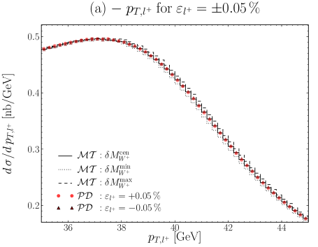
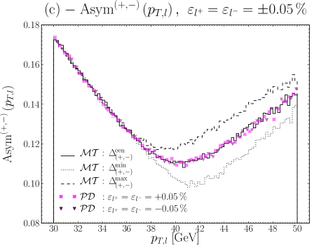
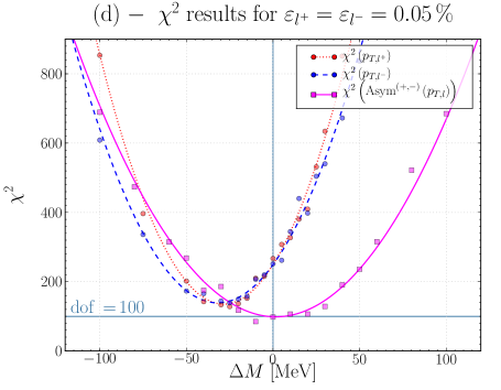
We start our detailed review on the energy scale systematics looking at the coherent biases. The plots above in Fig. 6.11 illustrate the consequences of coherent biases between the positively and negatively charged lepton reconstructed tracks. Fig. 6.11.(a) represents several distributions of the transverse momentum of the lepton. For the sake of clarity, only three mass templates from the entire collection have been drawn, the minimum template (), the central one () and the maximum one (). Although the histograms are considered for the analysis in the range of , a zoom was made on the jacobian peaks to make it possible to resolve by the eye the differences between the three . In top of these histograms the histograms corresponding to and are shown. For such values the deviation from is hardly decipherable. Fig. 6.11.(b) shows the exact same thing than in (a) but this time for the negative lepton. Fig. 6.11.(c) represents the charge asymmetry of for its central (), minimum () and maximum (). Are also present the two for which . Note here that the difference between the is much more magnified which is directly associated with the fact that the charge asymmetry, by its form, get rid of the common features from both and histograms and as a consequence emphasise the discrepancies among them. Note also that to decipher between the points of the two different , in each distribution a point is being skipped. Fig. 6.11.(d) presents the results for both classic and charge asymmetry methods for the case of . As seen in Table 6.9 both errors are quite steady with respect to the considered value of , nonetheless the convergence for the charge asymmetry method is slightly better than for the classic method.
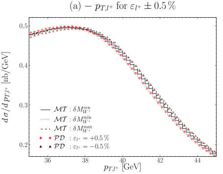
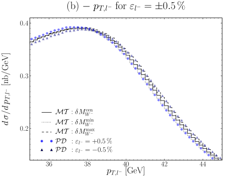
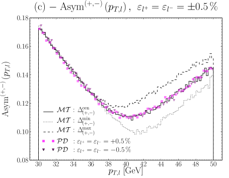
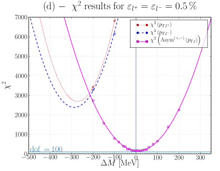
Now Fig. 6.12 represents the same histograms than in Fig. 6.11 but this time with . Now the bias is large enough so we can see some differences. Indeed, starting with Fig. 6.12.(a) the jacobian peaks of the are slightly shifted to higher for and to lower for . This can seem quite non intuitive but let us remind the biases are applied to , the inverse of , hence as long as , the bias on can be deduced at first order from the expression of :
| (6.31) |
justifying the inverse behaviour between and biases. Then, considering for example the case of , in both Figs. 6.12.(a) and (b) the jacobian peaks of the being shifted to lower both and are underestimated by as seen in frame (c). Nonetheless, since these biases are coherent the impact on is of the order of only. The low convergences is due to the lack of enough mass templates. In Fig. 6.12.(c) the charge asymmetry of the two show more steadiness than the bare spectra. Again for the sake of clarity in each distribution one point is being skipped each time. As expected the stability of the charge asymmetry with respect to biases of is such that the shows good convergence and no particular deviation from the central .
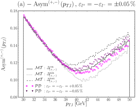
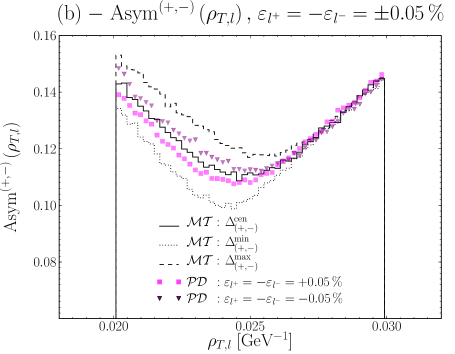
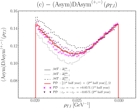
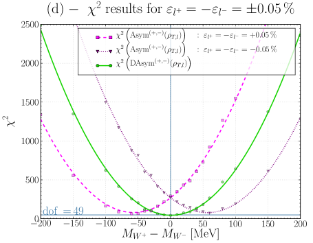
The incoherent biases for the energy scale between the positive and negative charged lepton is now addressed starting with Fig. 6.13 that considers the case of . This time the classic method is no longer treated since the are too much out of charts. Instead the charge and double charge asymmetry are confronted. First, Fig. 6.13.(a) shows the charge asymmetry of for the usual central and extrema and the two biased by energy scales of . In Fig. 6.13.(b) the same data is drawn in function of since it is in that space the is performed. Unlike the “coherent biases” here the deviation from the central are such that in (d) the systematic error are quite important, more precisely of the order of . Now in Fig. 6.13.(c) the case of the double charge asymmetry is considered in the space. The are exactly the same than the one used in (b), and the pseudo-data shows the cases where during the first year of the data collection and for the second half of the year due to the reversing of the solenoidal magnetic field of the tracker. Averaging the two data batches from the two six months period gives eventually a data collection which is localised near the central . The consequence can be seen in Fig. 6.13.(d), the double charge asymmetry is robust against such incoherent biases.
Finally, the “incoherent biases” are considered for as shown in Fig. 6.14. Here we can see the biased data are completely different from the templates. Nonetheless, for the double charge asymmetry the average of the two “six-months-data” gives again a total pseudo-data batch centered on the central distribution. Then, once again, the systematic error is still negligible for the double charge asymmetry while the charge asymmetry is not sufficient to draw any conclusion.
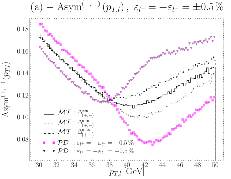
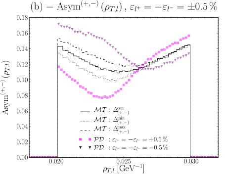
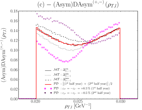
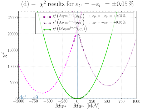
(b) Resolution of the charged lepton track parameters
The influence of the resolution of the charged lepton track are displayed in Fig. 6.15 for both (a,b) and charge asymmetry of (c). The value tends to narrow the bare distribution while having , by widening this time the width of the Gaussian response, tends to smear the sharpness of the distributions. Starting with the classic method we see that no matter which value is used here the bias on the intrinsic determination of and , and as a consequence on , is not very strong. We can note though that here in top of shifting the unbiased bare spectra to different the widening/narrowing change locally the normalisation. The consequence is that without any other technical refinement the can hardly apparent itself to any of the histogram. Also, even though the impact is negligible on the mass determination the convergence is very low, i.e. . In the frame (c) the charge asymmetry shows, no matter the used ERF values good steadiness and stays again in the vicinity of the central . Then, the result for the likelihood are good from both physics and convergence point of view.
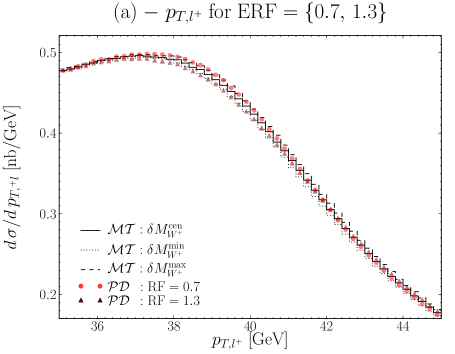
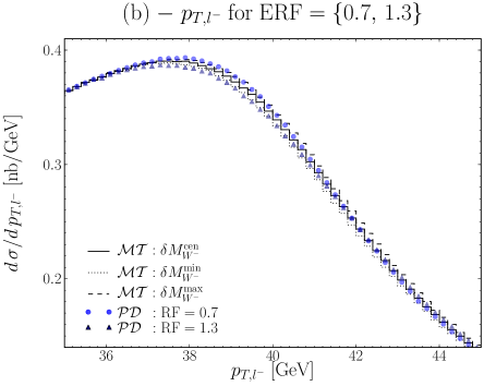
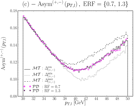
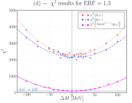
(c) Systematic due to the intrinsic of the partons
The impact of the intrinsic of partons is studied with the charge asymmetry method. First, Fig. 6.16 shows the impact of the change of on the jacobian peaks of the and spectra. As expected when the more important is the average intrinsic the more the jacobian peaks are shifted to higher values.
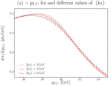
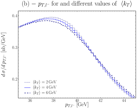
Fig. 6.17 on the next page presents in each frame the results for collisions with and respectively for the three following acceptance cuts :
-
,
-
and
-
.
The frames in Fig. 6.17 represent respectively the results obtained for these three cases and for the values of of , , , , and . The value is the central one but it was repeated to ensure the continuity in the pattern the follow as increases. The cuts made using , up to a lower convergence accuracy, displays a good steadiness with respect to the uncertainty on .
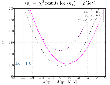
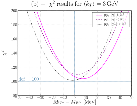
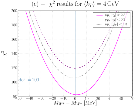
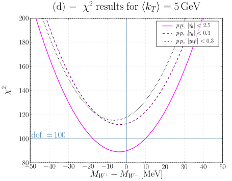
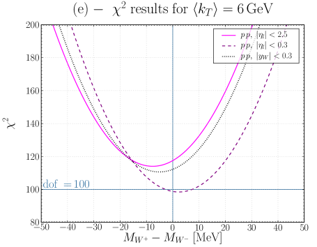
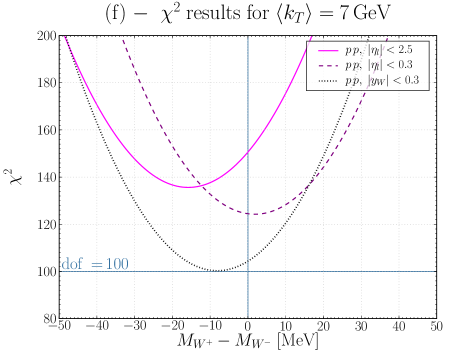
(d) asymmetry
Figure 6.18 presents the results obtained for the study of the asymmetry in the cases where and in (a) and where and in (b). The narrow selection on shows only a slight enhancement while the use of collisions, even with an acceptance of , remove the ambiguities on the valence PDF errors.
This can be understood quite easily looking at the impact of the modeled systematic error on the production of a and a for both and collisions. In the first case, for collision we consider the and are respectively produced via and . Making explicit the expressions of the biased valence distributions in functions of the LHAPDF (LHA) predictions gives
| (6.32) | |||||
| (6.33) |
where is the error on the PDF we’ve been introducing by hand. In this configuration we observe incoherent shift between the production of and . Now, for collisions we explicit this time the biased valence and expressions having in mind that in a neutron we have and . This leads to cancel incoherent biases between the and :
| (6.34) | |||||
| (6.35) | |||||
| (6.36) | |||||
| (6.37) | |||||
| (6.38) | |||||
| (6.39) |
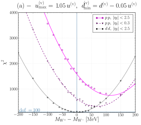
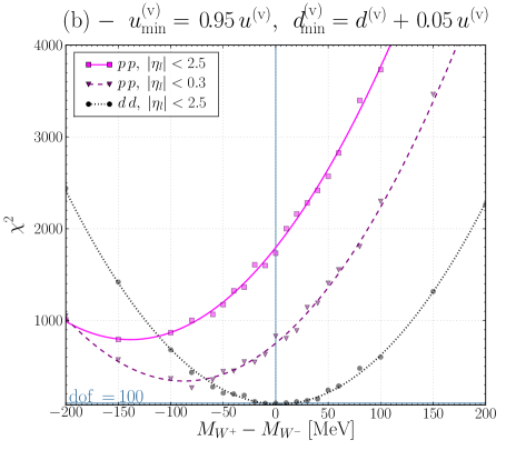
(e) asymmetry
Figure. 6.19 shows the results for the study of and in (a) and and in (b). In that case we see that having access to a narrow cut in the rapidity would improve a lot the independence from these quark flavours asymmetry in our measure.
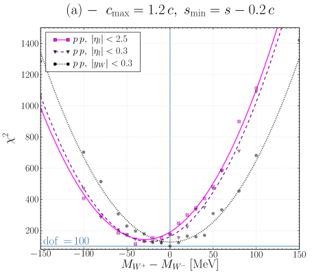
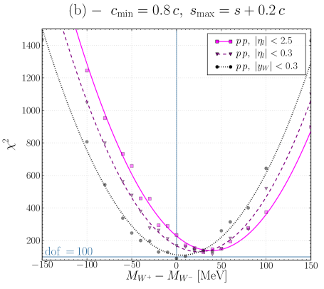
Chapter 7 Conclusion
Dobranoc, idȩ spać,
…Piosenka dla Edka
Maria Peszek
The work that has been presented in this document corresponds to the second stage in the optimisation of measurement strategies of the Standard Model parameters at the LHC. It presented a brand new dedicated strategy for the precision measurement of the charge asymmetry of the boson mass specific to the LHC collider physics.
This measurement must, in our view, precede the measurement of the charge averaged mass of the boson and the measurement of , in order to diminish the risk of false absorption of variety of unknown Beyond Standard Model effects within the Standard Model parameter space. This measurement is of particular importance for the following two reasons. Firstly, at the LHC – contrary to the Tevatron collider – we have seen the measurement of the averaged mass of the boson cannot be dissociated from the measurement of the masses of its charge states. Secondly, the precision of verification of the charge universality of the Fermi coupling constant , measured via the charge asymmetry of the muon life time, must be matched by the precision of verification of the charge universality of the coupling strength . This can be achieved only if the mass difference can be determined with the precision of a few MeV, i.e. a factor of better than the best present measurement.
The Tevatron collision scheme, as far as the systematic and modeling errors are concerned, is better suited for the precision measurement of the boson charge asymmetry. However, even if dedicated strategies, as e.g. those proposed in this document are used, the measurement will be limited by the statistical precision, affecting both the boson samples and, more importantly, the boson calibration sample.
At the LHC the requisite statistical precision can be achieved already for the integrated luminosity of , i.e. in the first year of the LHC operation at the “low”, , luminosity. However, in order to achieve a comparable systematic precision in an analysis based on the calibration and measurement strategies developed at the Tevatron, the charge dependent biases in the energy (momentum) scale of positive (negative) leptons must be controlled to the precision of . As it was argued, it will be extremely hard, if not impossible, to achieve such a precision using the calibration methods developed at the Tevatron. Moreover, we have identified the LHC-specific sources of errors, related to the uncertainties in the present knowledge of the flavour composition of the WBpB which limit, at present, the measurement precision to . Certainly, this uncertainty will be reduced once the high statistic boson and boson samples are collected. Nevertheless, it will be hard, if not impossible, to improve by a factor of 10 or more the precision of the – and – quark-momentum distribution asymmetries, as they are hardly detectable in the -boson production processes. Whether or not the requisite precision target will be reached using the standard measurement strategies remains to be seen. In our view, it will be indispensable to use the dedicated LHC-specific measurement strategies.
The strategy proposed and discussed here makes a full use of the flexibility of the machine and detector configurations which, we hope, will be exploited in the mature phase of the LHC experimental program. It requires : (1) running for a fraction of time the inverted polarity current in the detector solenoid, (2) the dedicated trigger and data-acquisition configuration in the “high”, , luminosity LHC operation mode, and (3) replacing the LHC proton beams by light isoscalar ion beams.
The underlying principle of the proposed dedicated strategy is that, instead of diminishing the systematic measurement and modeling uncertainties, it minimizes their influence on the measured value of . We have demonstrated that already for the modest (easy to fulfill) measurement and modeling precision requirements, the resulting uncertainty of can be kept at the level comparable to the statistical measurement uncertainty, i.e. at the level of .
It remains to be demonstrated that the remaining systematic measurement errors, of secondary importance at the Tevatron and not discussed here, could be neglected at this level of the measurement precision. This can, however, be proved only when the real data are collected and analysed, both for the standard and for the dedicated measurement strategies.
References
- [1] Particle Data Group Collaboration, C. Amsler et. al., Review of particle physics, Phys. Lett. B667 (2008) 1.
- [2] J. Thomson, Cathode Rays, Phil. Mag. 44 (1897) 292.
- [3] W. Kaufmann Ann. Phys. 61 (1897) 544.
- [4] W. Kaufmann Ann. Phys. 62 (1897) 588.
- [5] S. H. Neddermeyer and C. D. Anderson, Note on the nature of cosmic-ray particles, Phys. Rev. 51 (May, 1937) 884–886.
- [6] M. L. Perl, G. S. Abrams, A. M. Boyarski, M. Breidenbach, D. D. Briggs, F. Bulos, W. Chinowsky, J. T. Dakin, G. J. Feldman, C. E. Friedberg, D. Fryberger, G. Goldhaber, G. Hanson, F. B. Heile, B. Jean-Marie, J. A. Kadyk, R. R. Larsen, A. M. Litke, D. Lüke, B. A. Lulu, V. Lüth, D. Lyon, C. C. Morehouse, J. M. Paterson, F. M. Pierre, T. P. Pun, and P. A. Rapidis, Evidence for anomalous lepton production in annihilation, Phys. Rev. Lett. 35 (Dec, 1975) 1489–1492.
- [7] F. Reines and C. L. Cowan, Detection of the free neutrino, Phys. Rev. 92 (1953) 830–831.
- [8] G. Danby et. al., Observation of High-Energy Neutrino Reactions and the Existence of Two Kinds of Neutrinos, Phys. Rev. Lett. 9 (1962) 36–44.
- [9] K. Kodama et. al., Detection and analysis of tau neutrino interactions in DONUT emulsion target, Nucl. Instrum. Meth. A493 (2002) 45–66.
- [10] H. W. Kendall, Deep inelastic scattering: Experiments on the proton and the observation of scaling, Rev. Mod. Phys. 63 (Jul, 1991) 597–614.
- [11] T. Eichten et. al., Measurement of the neutrino - nucleon anti-neutrino - nucleon total cross-sections, Phys. Lett. B46 (1973) 274–280.
- [12] J. J. Aubert, U. Becker, P. J. Biggs, J. Burger, M. Chen, G. Everhart, P. Goldhagen, J. Leong, T. McCorriston, T. G. Rhoades, M. Rohde, S. C. C. Ting, S. L. Wu, and Y. Y. Lee, Experimental observation of a heavy particle , Phys. Rev. Lett. 33 (Dec, 1974) 1404–1406.
- [13] SLAC-SP-017 Collaboration, J. E. Augustin et. al., Discovery of a Narrow Resonance in e+ e- Annihilation, Phys. Rev. Lett. 33 (1974) 1406–1408.
- [14] S. W. Herb et. al., Observation of a dimuon resonance at 9.5-GeV in 400-GeV proton - nucleus collisions, Phys. Rev. Lett. 39 (1977) 252–255.
- [15] CDF Collaboration, F. Abe et. al., Observation of top quark production in collisions, Phys. Rev. Lett. 74 (1995) 2626–2631, [hep-ex/9503002].
- [16] D0 Collaboration, S. Abachi et. al., Observation of the top quark, Phys. Rev. Lett. 74 (1995) 2632–2637, [hep-ex/9503003].
- [17] A. Einstein, Concerning an heuristic point of view toward the emission and transformation of light, Annalen Phys. 17 (1905) 132–148.
- [18] UA1 Collaboration, G. Arnison et. al., Experimental observation of isolated large transverse energy electrons with associated missing energy at s**(1/2) = 540-GeV, Phys. Lett. B122 (1983) 103–116.
- [19] UA2 Collaboration, M. Banner et. al., Observation of single isolated electrons of high transverse momentum in events with missing transverse energy at the CERN anti-p p collider, Phys. Lett. B122 (1983) 476–485.
- [20] UA1 Collaboration, G. Arnison et. al., Experimental observation of lepton pairs of invariant mass around 95-GeV/c**2 at the CERN SPS collider, Phys. Lett. B126 (1983) 398–410.
- [21] UA2 Collaboration, P. Bagnaia et. al., Evidence for Z0 –¿ e+ e- at the CERN anti-p p collider, Phys. Lett. B129 (1983) 130–140.
- [22] TASSO Collaboration, R. Brandelik et. al., Evidence for Planar Events in e+ e- Annihilation at High- Energies, Phys. Lett. B86 (1979) 243.
- [23] D. P. Barber et. al., Discovery of Three Jet Events and a Test of Quantum Chromodynamics at PETRA Energies, Phys. Rev. Lett. 43 (1979) 830.
- [24] PLUTO Collaboration, C. Berger et. al., Evidence for Gluon Bremsstrahlung in e+ e- Annihilations at High-Energies, Phys. Lett. B86 (1979) 418.
- [25] M. Gell-Mann, A Schematic Model of Baryons and Mesons, Phys. Lett. 8 (1964) 214–215.
- [26] G. Zweig, An SU(3) model for strong interaction symmetry and its breaking, . Reprinted in Lichtenberg, D. B. ( Ed.), Rosen, S. P. ( Ed.) : Developments In The Quark Theory Of Hadrons, Vol. I, 22-101 and CERN Geneva - TH. 401 (REC.JAN. 64) 24p.
- [27] D. J. Gross and F. Wilczek, Asymptotically Free Gauge Theories. 1, Phys. Rev. D8 (1973) 3633–3652.
- [28] D. J. Gross and F. Wilczek, Asymptotically free gauge theories. 2, Phys. Rev. D9 (1974) 980–993.
- [29] H. D. Politzer, Reliable perturbative results for strong interactions?, Phys. Rev. Lett. 30 (1973) 1346–1349.
- [30] V. N. Gribov and L. N. Lipatov, Deep inelastic e p scattering in perturbation theory, Sov. J. Nucl. Phys. 15 (1972) 438–450.
- [31] G. Altarelli and G. Parisi, Asymptotic Freedom in Parton Language, Nucl. Phys. B126 (1977) 298.
- [32] Y. L. Dokshitzer, Calculation of the Structure Functions for Deep Inelastic Scattering and Annihilation by Perturbation Theory in Quantum Chromodynamics. (In Russian), Sov. Phys. JETP 46 (1977) 641–653.
- [33] S. L. Glashow, Partial Symmetries of Weak Interactions, Nucl. Phys. 22 (1961) 579–588.
- [34] A. Salam and J. C. Ward, Electromagnetic and weak interactions, Phys. Lett. 13 (1964) 168–171.
- [35] S. Weinberg, A Model of Leptons, Phys. Rev. Lett. 19 (1967) 1264–1266.
- [36] F. Englert and R. Brout, Broken symmetry and the mass of gauge vector mesons, Phys. Rev. Lett. 13 (1964) 321–322.
- [37] P. W. Higgs, Broken symmetries, massless particles and gauge fields, Phys. Lett. 12 (1964) 132–133.
- [38] G. S. Guralnik, C. R. Hagen, and T. W. B. Kibble, Global conservation laws and massless particles, Phys. Rev. Lett. 13 (1964) 585–587.
- [39] N. Cabibbo, Unitary Symmetry and Leptonic Decays, Phys. Rev. Lett. 10 (1963) 531–533.
- [40] M. Kobayashi and T. Maskawa, CP Violation in the Renormalizable Theory of Weak Interaction, Prog. Theor. Phys. 49 (1973) 652–657.
- [41] G. Cohen-Tannoudji, “Une bréve introduction au modèle standard.” In “Congrès de la Société Française de Physique - Strasbourg 9–13 juillet 2001”.
- [42] I. J. R. Aitchison and A. J. G. Hey, Gauge Theories in Particle Physics a practical introduction. Volume 1 : from relativistic quantum mechanics to QED, (3rd Ed.). Institute of Physics Publishing, 2002. Erratum and addendum : http://www.slac.stanford.edu/~aitchiso/.
- [43] I. J. R. Aitchison and A. J. G. Hey, Gauge Theories in Particle Physics a practical introduction. Volume 2 : QCD and the Electroweak Theory, (3rd Ed.). Institute of Physics Publishing, 2004. Erratum and addendum : http://www.slac.stanford.edu/~aitchiso/.
- [44] L. H. Ryder, Quantum Field Theory, (2nd Ed.). Cambridge University Press, 1996.
- [45] M. E. Peskin and D. V. Schroeder, An Introduction to Quantum Field Theory. Reading, USA : Addison-Wesley, 1995. Erratum and addendum : http://www.slac.stanford.edu/~mpeskin/QFT.html.
- [46] R. K. Ellis, W. J. Stirling, and B. R. Webber, QCD and collider physics. Camb. Monogr. Part. Phys. Nucl. Phys. Cosmol., 1996.
- [47] H. Spiesberger, M. Spira, and P. M. Zerwas, The Standard model : Physical basis and scattering experiments, hep-ph/0011255.
- [48] W. Pauli, Niels Bohr and the development of Physics. Pergamon Press, London, 1955.
- [49] CERN-Mainz-Daresbury Collaboration, J. Bailey et. al., Final Report on the CERN Muon Storage Ring Including the Anomalous Magnetic Moment and the Electric Dipole Moment of the Muon, and a Direct Test of Relativistic Time Dilation, Nucl. Phys. B150 (1979) 1.
- [50] Muon g-2 Collaboration, G. W. Bennett et. al., Measurement of the negative muon anomalous magnetic moment to 0.7-ppm, Phys. Rev. Lett. 92 (2004) 161802, [hep-ex/0401008].
- [51] CDF Collaboration, T. Aaltonen et. al., First Run II Measurement of the Boson Mass, Phys. Rev. D77 (2008) 112001, [arXiv:0708.3642].
- [52] CDF Collaboration, F. Abe et. al., A Measurement of the Boson Mass, Phys. Rev. Lett. 65 (1990) 2243–2246.
- [53] CDF Collaboration, F. Abe et. al., A Measurement of the Boson Mass in 1.8 TeV Collisions, Phys. Rev. D43 (1991) 2070–2093.
- [54] CDF Collaboration, F. Abe et. al., Measurement of the boson mass, Phys. Rev. Lett. 75 (1995) 11–16, [hep-ex/9503007].
- [55] CDF Collaboration, F. Abe et. al., Measurement of the boson mass, Phys. Rev. D52 (1995) 4784–4827.
- [56] CDF Collaboration, T. Aaltonen et. al., First Measurement of the Boson Mass in Run II of the Tevatron, Phys. Rev. Lett. 99 (2007) 151801, [arXiv:0707.0085].
- [57] V. Buge et. al., Prospects for the precision measurement of the W mass with the CMS detector at the LHC, J. Phys. G34 (2007) N193–N220.
- [58] ATLAS Collaboration, N. Besson, M. Boonekamp, E. Klinkby, T. Petersen, and S. Mehlhase, Re-evaluation of the LHC potential for the measurement of Mw, Eur. Phys. J. C57 (2008) 627–651, [arXiv:0805.2093].
- [59] F. Halzen and A. D. Martin, Quarks And Leptons : An Introductory Course In Modern Particle Phyics. New York, USA : Wiley, 1984.
- [60] S. D. Drell and T.-M. Yan, Partons and their applications at high energies, Ann. Phys. 66 (1971) 578.
- [61] V. Barger and R. Phillips, Collider physics. Addison-Wesley, 1990.
- [62] P. M. Nadolsky, Theory of and boson production, AIP Conf. Proc. 753 (2005) 158–170, [hep-ph/0412146].
- [63] U. Baur, S. Keller, and D. Wackeroth, Electroweak radiative corrections to boson production in hadronic collisions, Phys. Rev. D59 (1999) 013002, [hep-ph/9807417].
- [64] F. A. Berends and R. Kleiss, Hard photon effects in and decay, Z. Phys. C27 (1985) 365.
- [65] S. Dittmaier and M. Kramer, Electroweak radiative corrections to -boson production at hadron colliders, Phys. Rev. D65 (2002) 073007, [hep-ph/0109062].
- [66] J. Pumplin et. al., New generation of parton distributions with uncertainties from global QCD analysis, JHEP 07 (2002) 012, [hep-ph/0201195].
- [67] A. Bodek, Y. Chung, B.-Y. Han, K. McFarland, and E. Halkiadakis, Direct measurement of Production Charge Asymmetry at the Tevatron, Phys. Rev. D77 (2008) 111301, [arXiv:0711.2859].
- [68] K. Lohwasser, to be published. PhD thesis, Oxford University.
- [69] W. L. van Neerven, J. A. M. Vermaseren, and K. J. F. Gaemers, Lepton–jet events as a signature for production in collisions, NIKHEF-H/82-20 (November, 1982).
- [70] J. Smith, W. L. van Neerven, and J. A. M. Vermaseren, The transverse mass and width of the boson, Phys. Rev. Lett. 50 (1983) 1738.
- [71] ATLAS Collaboration, G. Aad et. al., Expected Performance of the ATLAS Experiment - Detector, Trigger and Physics, arXiv:0901.0512.
- [72] M. W. Krasny, F. Fayette, W. Płaczek, and A. Siódmok, Measure of the -boson mass in the ATLAS experiment., in prepration.
- [73] A. K. Siódmok, Theoretical predictions for the Drell–Yan process at LHC using Monte Carlo methods. PhD thesis, Jagelionan University, 2009.
- [74] K. Rejzner, M. W. Krasny, F. Fayette, W. Płaczek, and A. Siódmok, Measure of the -boson width in the ATLAS experiment, in prepration.
- [75] A. Asner et. al., The Large Hadron Collider in the lep tunnel, CERN-87-05.
- [76] O. S. Brüning et. al., LHC Design Report, v.1, CERN-2004-003-V-1 (2004).
- [77] O. S. Brüning et. al., LHC Design Report, v.2, CERN-2004-003-V-2 (2004).
- [78] “Large hadron collider homepage.” http://lhc.web.cern.ch.
- [79] LHC Machine, JINST 3 (2008) S08001.
- [80] “CERN Homepage.” http://public.web.cern.ch.
- [81] ATLAS Collaboration, W. Armstrong, W. et. al., ATLAS: Technical proposal for a general-purpose experiment at the Large Hadron Collider at CERN, CERN-LHCC-94-43.
- [82] ATLAS Collaboration, G. Aad et. al., The ATLAS Experiment at the CERN Large Hadron Collider, JINST 3 (2008) S08003.
- [83] The Lep Injector Study Group Collaboration, LEP design report. vol. 1, CERN-LEP/TH/83-29 (1983) 70.
- [84] A. Asner et. al., Large Hadron Collider in the LEP tunnel: a feasibility study of possible options by the cern machine group, CERN-DIR-TECH-84-01.
- [85] CMS Collaboration, R. Adolphi et. al., The CMS experiment at the CERN LHC, JINST 3 (2008) S08004.
- [86] ALICE Collaboration, K. Aamodt et. al., The ALICE experiment at the CERN LHC, JINST 3 (2008) S08002.
- [87] LHCb Collaboration, A. A. Alves et. al., The LHCb Detector at the LHC, JINST 3 (2008) S08005.
- [88] LHCf Collaboration, O. Adriani et. al., The LHCf detector at the CERN Large Hadron Collider, JINST 3 (2008) S08006.
- [89] TOTEM Collaboration, G. Anelli et. al., The TOTEM experiment at the CERN Large Hadron Collider, JINST 3 (2008) S08007.
- [90] ATLAS Collaboration, ATLAS liquid argon calorimeter: Technical design report, .
- [91] ATLAS Collaboration, A. Airapetian et. al., ATLAS calorimeter performance, CERN-LHCC-96-40.
- [92] ATLAS Electromagnetic Barrel Calorimeter Collaboration, M. Aharrouche et. al., Energy linearity and resolution of the ATLAS electromagnetic barrel calorimeter in an electron test- beam, Nucl. Instrum. Meth. A568 (2006) 601–623, [physics/0608012].
- [93] ATLAS Collaboration, Physics performance studies and strategy of the Electron and Photon Trigger Selection, ATLAS-PHYS-PUB-2007-000 (2008).
- [94] ATLAS Collaboration, ATLAS tile calorimeter: Technical design report, CERN-LHCC-96-42.
- [95] K. Störig, J. Grosse-Knetter, K. Kröninger, and A. Quadt, Alignment Studies of the ATLAS Silicon Trackers with Overlap Residuals, com-indet-2008-012.
- [96] ATLAS Collaboration, ATLAS inner detector: Technical design report. Vol. 1, . CERN-LHCC-97-16.
- [97] ATLAS Collaboration, ATLAS inner detector: Technical design report. Vol. 2, CERN-LHCC-97-17.
- [98] ATLAS Collaboration, ATLAS CSC note : The expected performance of the ATLAS tracker, COM-PHYS-2008-105 (2008).
- [99] ATLAS Collaboration, ATLAS: Detector and physics performance technical design report. Volume 1, CERN-LHCC-99-14.
- [100] A. Yamamoto et. al., The ATLAS central solenoid, Nucl. Instrum. Meth. A584 (2008) 53–74.
- [101] C. J. S. Damerell, Vertex detectors: The State of the art and future prospects, Lectures given at 23rd Annual SLAC Summer Institute on Particle Physics: The Top Quark and the Electroweak Interaction, Stanford, CA, 10-21 Jul 1995.
- [102] I. Gorelov et. al., A measurement of Lorentz angle and spatial resolution of radiation hard silicon pixel sensors, Nucl. Instrum. Meth. A481 (2002) 204–221.
- [103] T. G. Cornelissen, Track fitting in the ATLAS experiment. PhD thesis, Faculteit der Natuurwetenschappen, Wiskunde en Informatica, December, 2006. CERN-THESIS-2006-072.
- [104] T. Cornelissen et. al., Concepts, Design and Implementation of the ATLAS New Tracking (NEWT), CERN-LHCC-99-14.
- [105] R. Fruhwirth, Application of Kalman filtering to track and vertex fitting, Nucl. Instrum. Meth. A262 (1987) 444–450.
- [106] P. Brückman de Renstrom and S. Haywood, Least squares approach to the alignment of the generic high precision tracking system, Prepared for PHYSTATO5: Statistical Problems in Particle Physics, Astrophysics and Cosmology, Oxford, England, United Kingdom, 12-15 Sep 2005.
- [107] D. Brown, A. Gritsan, and D. Roberts, Internal alignment of the BABAR silicon vertex tracking detector, Prepared for 1st LHC Detection Alignment Workshop, Geneva, Switzerland, 4-6 Sep 2006.
- [108] K. Störig, Alignment Studies of the ATLAS Silicon Trackers with Overlap Residuals. PhD thesis, Georg-August-Universität Götingen, April, 2008.
- [109] CDF IIb Collaboration, P. T. Lukens, The CDF IIb detector: Technical design report, FERMILAB-TM-2198.
- [110] ATLAS Collaboration, ATLAS detector and physics performance. Technical design report. Vol. 2, CERN-LHCC-99-15.
- [111] P. Brückman de Restrom, “About the weak modes of the atlas tracker.” private communication, 2008.
- [112] CDF Collaboration, A. A. Affolder et. al., CDF central outer tracker, Nucl. Instrum. Meth. A526 (2004) 249–299.
- [113] N. Metropolis and S. Ulam, The Monte Carlo method, Journal of the American Statistical Association 44 (1949) 335–341.
- [114] Press, William, H. and Teukolsky, Saul, A.and Vetterling, William, T. and Flannery, Brian, P., Numerical Recipes : The Art of Scientific Computing.
- [115] T. Sjöstrand, Academic Training Lectures, April, 2005. http://home.thep.lu.se/~torbjorn/talks/cern05lecture1.pdf.
- [116] D. E. Knuth, The Art of Computer Programming. Vol. 2 Semi-numerical algorithms. Addison Wesley, 1981.
- [117] T. Sjöstrand, S. Mrenna, and P. Skands, Pythia 6.4 physics and manual, JHEP 05 (2006) 026, [hep-ph/0603175].
- [118] T. Sjöstrand, Pythia 8 Status Report, arXiv:0809.0303.
- [119] “Homepage of the Pythia Event Generator.” http://home.thep.lu.se/~torbjorn/Pythia.html.
- [120] M. Bähr et. al., Herwig++ Physics and Manual, Eur. Phys. J. C58 (2008) 639–707, [arXiv:0803.0883].
- [121] “Homepage of the Herwig++ Event Generator.” http://projects.hepforge.org/herwig/.
- [122] T. Gleisberg et. al., SHERPA 1.alpha, a proof-of-concept version, JHEP 02 (2004) 056, [hep-ph/0311263].
- [123] “Homepage of the Sherpa Event Generator.” www.montecarlonet.org/index.php?p=Projects/sherpa or http://projects.hepforge.org/sherpa/dokuwiki/doku.php.
- [124] E. Barberio, B. van Eijk, and Z. Was, PHOTOS: A Universal Monte Carlo for QED radiative corrections in decays, Comput. Phys. Commun. 66 (1991) 115–128.
- [125] E. Barberio and Z. Was, PHOTOS: A Universal Monte Carlo for QED radiative corrections. Version 2.0, Comput. Phys. Commun. 79 (1994) 291–308.
- [126] P. Golonka and Z. Was, Next to leading logarithms and the PHOTOS Monte Carlo, Eur. Phys. J. C50 (2007) 53–62, [hep-ph/0604232].
- [127] S. Jadach, J. H. Kuhn, and Z. Was, TAUOLA: A Library of Monte Carlo programs to simulate decays of polarized tau leptons, Comput. Phys. Commun. 64 (1990) 275–299.
- [128] M. Jezabek, Z. Was, S. Jadach, and J. H. Kuhn, The tau decay library TAUOLA, update with exact QED corrections in tau mu. (e) neutrino anti-neutrino decay modes, Comput. Phys. Commun. 70 (1992) 69–76.
- [129] S. Jadach, Z. Was, R. Decker, and J. H. Kuhn, The tau decay library TAUOLA: Version 2.4, Comput. Phys. Commun. 76 (1993) 361–380.
- [130] A. Djouadi, J. Kalinowski, and M. Spira, HDECAY: A program for Higgs boson decays in the standard model and its supersymmetric extension, Comput. Phys. Commun. 108 (1998) 56–74, [hep-ph/9704448].
- [131] H. Seymour, Michael, Prediction for Higgs and Electroweak Boson Production. PhD thesis, University of Cambridge, October, 1992. http://hepwww.rl.ac.uk/theory/seymour/thesis/.
- [132] T. Sjöstrand, Monte Carlo generators, hep-ph/0611247.
- [133] T. Sjöstrand, “CERN Academic training lectures.” http://home.thep.lu.se/~torbjorn/talks/.
- [134] M. Seymour, “CERN Academic training lectures.” http://seymour.web.cern.ch/seymour/slides/.
- [135] W. Płaczek, Monte Carlo Methods in High Energy Physics - lectures given at the INFN Pavia and the University of Pavia, Italy,, Ocotober, 2004. http://placzek.web.cern.ch/placzek/lectures/.
- [136] CTEQ, “Links to talks given during CTEQ Summer Schools.” http://www.phys.psu.edu/~cteq/#Summer.
- [137] Talk given by J.D. Bjorken at the 75th anniversary celebration of the Max-Planck Institute of Physics, Munich, Germany, December 10th, 1992. As quoted in: Beam Line, Winter 1992, Vol. 22, No. 4.
- [138] Dissertori, Günther and Knowles, Ian G. and Schmelling, Michael, Quantum Chromodynamics : High Energy Experiments and Theory. Clarendon Press, 2003.
- [139] W. Płaczek and S. Jadach, Multiphoton radiation in leptonic -boson decays, Eur. Phys. J. C29 (2003) 325–339, [hep-ph/0302065].
- [140] C. M. Carloni Calame, S. Jadach, G. Montagna, O. Nicrosini, and W. Płaczek, Comparisons of the Monte Carlo programs HORACE and WINHAC for single -boson production at hadron colliders, Acta Phys. Polon. B35 (2004) 1643–1674, [hep-ph/0402235].
- [141] TeV4LHC-Top and Electroweak Working Group Collaboration, C. E. Gerber et. al., Tevatron-for-LHC Report : Top and Electroweak Physics, arXiv:0705.3251.
- [142] D. Bardin, S. Bondarenko, S. Jadach, L. Kalinovskaya, and W. Placzek, Implementation of SANC EW corrections in WINHAC Monte Carlo generator, arXiv:0806.3822.
- [143] P. Golonka and Z. Was, PHOTOS Monte Carlo: A precision tool for QED corrections in and decays, Eur. Phys. J. C45 (2006) 97–107, [hep-ph/0506026].
- [144] M. W. Krasny, S. Jadach, and W. Płaczek, The femto-experiment for the LHC : The -boson beams and their targets, Eur. Phys. J. C44 (2005) 333–350, [hep-ph/0503215].
- [145] M. W. Krasny, F. Fayette, W. Płaczek, and A. Siódmok, Z-boson as ’the standard candle’ for high precision -boson physics at LHC, Eur. Phys. J. C51 (2007) 607–617, [hep-ph/0702251].
- [146] F. Fayette, M. W. Krasny, W. Placzek, and A. Siódmok, Measurement of at the LHC, arXiv:0812.2571.
- [147] W. Płaczek and S. Jadach, “WINHAC version 1.30: The Monte Carlo event generator for single -boson production with leptonic decays in hadron collisions.” available from http://cern.ch/placzek/winhac.
- [148] D. R. Yennie, S. Frautschi, and H. Suura Ann. Phys. (NY) 13 (1961) 379.
- [149] M. R. Whalley, D. Bourilkov, and R. C. Group, The Les Houches Accord PDFs (LHAPDF) and Lhaglue, hep-ph/0508110.
- [150] H. Plothow-Besch, PDFLIB: A Library of all available parton density functions of the nucleon, the pion and the photon and the corresponding alpha-s calculations, Comput. Phys. Commun. 75 (1993) 396–416.
- [151] K. J. Eskola, V. J. Kolhinen, and C. A. Salgado, The scale dependent nuclear effects in parton distributions for practical applications, Eur. Phys. J. C9 (1999) 61–68, [hep-ph/9807297].
- [152] K. J. Eskola, V. J. Kolhinen, and P. V. Ruuskanen, Scale evolution of nuclear parton distributions, Nucl. Phys. B535 (1998) 351–371, [hep-ph/9802350].
- [153] A. Siódmok and W. Płaczek, “ZINHAC: The Monte Carlo event generator for single -boson production with leptonic decays in hadron collisions.” in preparation.
- [154] F. James, A Review of Pseudorandom Number Generators, Comput. Phys. Commun. 60 (1990) 329–344.
- [155] G. Marsaglia, A. Zaman, and W.-W. Tsang, A Review of Pseudorandom Number Generators, Stat.Prob. Lett. 9 (1990) 35.
- [156] C. M. Carloni Calame, G. Montagna, O. Nicrosini, and M. Treccani, Higher-order QED corrections to W-boson mass determination at hadron colliders, Phys. Rev. D69 (2004) 037301, [hep-ph/0303102].
- [157] “Homepage of the HORACE Event Generator.” http://www.pv.infn.it/~hepcomplex/horace.html.
- [158] G. Corcella et. al., HERWIG 6.5: an event generator for Hadron Emission Reactions With Interfering Gluons (including supersymmetric processes), JHEP 01 (2001) 010, [hep-ph/0011363].
- [159] “Homepage of the HERWIG Event Generator.” http://hepwww.rl.ac.uk/theory/seymour/herwig/herwig65.html.
- [160] S. Frixione and B. R. Webber, Matching NLO QCD computations and parton shower simulations, JHEP 06 (2002) 029, [hep-ph/0204244].
- [161] “Homepage of the MC@NLO Event Generator.” http://www.hep.phy.cam.ac.uk/theory/webber/MCatNLO/.
- [162] B. P. Kersevan and E. Richter-Was, The Monte Carlo event generator AcerMC version 2.0 with interfaces to PYTHIA 6.2 and HERWIG 6.5, hep-ph/0405247.
- [163] “Homepage of the AcerMC Event Generator.” http://borut.home.cern.ch/borut/.
- [164] Q.-H. Cao and C. P. Yuan, Combined effect of QCD resummation and QED radiative correction to W boson observables at the Tevatron, Phys. Rev. Lett. 93 (2004) 042001, [hep-ph/0401026].
- [165] “Homepage of the ResBos-A Event Generator.” http://hep.pa.msu.edu/people/cao/ResBos-A.html.
- [166] C. Balazs and C. P. Yuan, Soft gluon effects on lepton pairs at hadron colliders, Phys. Rev. D56 (1997) 5558–5583, [hep-ph/9704258].
- [167] “Homepage of the ResBos Event Generator.” http://www.pa.msu.edu/~balazs/ResBos/.
- [168] “Homepage of the WGRAD Event Generator.” http://ubpheno.physics.buffalo.edu/~dow/wgrad.html.
- [169] U. Baur, O. Brein, W. Hollik, C. Schappacher, and D. Wackeroth, Electroweak radiative corrections to neutral-current Drell-Yan processes at hadron colliders, Phys. Rev. D65 (2002) 033007, [hep-ph/0108274].
- [170] “Homepage of the ZGRAD2 Event Generator.” http://ubpheno.physics.buffalo.edu/~dow/.
- [171] A. Arbuzov et. al., One-loop corrections to the Drell-Yan process in SANC. I: The charged current case, Eur. Phys. J. C46 (2006) 407–412, [hep-ph/0506110].
- [172] “Homepage of the SANC Event Generator.” http://sanc.jinr.ru or http://pcphsanc.cern.ch/.
- [173] W. T. Giele, E. W. N. Glover, and D. A. Kosower, Higher order corrections to jet cross-sections in hadron colliders, Nucl. Phys. B403 (1993) 633–670, [hep-ph/9302225].
- [174] ATLAS Collaboration, ATLAS computing: Technical design report, CERN-LHCC-2005-022.
- [175] ATLAS Collaboration, “ATLAS Computing Workbook.” https://twiki.cern.ch/twiki/bin/view/Atlas/WorkBook.
- [176] G. Barrand et. al., GAUDI - The software architecture and framework for building LHCb data processing applications, Prepared for International Conference on Computing in High- Energy Physics and Nuclear Physics (CHEP 2000), Padova, Italy, 7-11 Feb 2000.
- [177] G. Barrand et. al., GAUDI - A software architecture and framework for building HEP data processing applications, Comput. Phys. Commun. 140 (2001) 45–55.
- [178] R. Brun and F. Rademakers, ROOT: An object oriented data analysis framework, Nucl. Instrum. Meth. A389 (1997) 81–86.
- [179] “The ROOT System Homepage.” http://root.cern.ch/.
- [180] E. Richter-W as, F. Daniel, and P. Luc, ATLFAST 2.0 a fast simulation package for ATLAS, ATL-PHYS-98-131 (October, 1998).
- [181] Cavalli, D and others, Performance of the ATLAS fast simulation ATLFAST, ATL-PHYS-INT-2007-005, ATL-COM-PHYS-2007-012 (January, 2007).
- [182] “Atlfast homepage.” http://www.hep.ucl.ac.uk/atlas/atlfast/.
- [183] “Generator Services Subproject.” http://lcgapp.cern.ch/project/simu/generator/.
- [184] “CLHEP - A Class Library for High Energy Physics.” http://proj-clhep.web.cern.ch/proj-clhep/.
- [185] M. Dobbs and J. B. Hansen, The HepMC C++ Monte Carlo event record for High Energy Physics, Comput. Phys. Commun. 134 (2001) 41–46.
- [186] GEANT4 Collaboration, S. Agostinelli et. al., GEANT4: A simulation toolkit, Nucl. Instrum. Meth. A506 (2003) 250–303.
- [187] J. Allison et. al., Geant4 developments and applications, IEEE Trans. Nucl. Sci. 53 (2006) 270.
- [188] M. A. Dobbs et. al., Les Houches guidebook to Monte Carlo generators for hadron collider physics, hep-ph/0403045.
- [189] F. Fayette and G. Stavropoulos, Implementation of WINHAC inside the Athena framework, October, 2006. http://indico.cern.ch/materialDisplay.py?contribId=2&materialId=slides%&confId=6357.
- [190] F. Fayette and G. Stavropoulos, Report on Winhac_i validations status, October, 2006. http://indico.cern.ch/materialDisplay.py?contribId=3&materialId=slides%&confId=6872.
- [191] D. Adams and others, Track Reconstruction in the ATLAS Muon Spectrometer with MOORE, ATL-SOFT-2003-007, ATL-COM-MUON-2003-012 (2003).
- [192] D. Stump et. al., Inclusive jet production, parton distributions, and the search for new physics, JHEP 10 (2003) 046, [hep-ph/0303013].
- [193] S. Gieseke, M. H. Seymour, and A. Siódmok, A model of non-perturbative gluon emission in an initial state parton shower, JHEP 06 (2008) 001, [arXiv:0712.1199].
- [194] H1 Collaboration, D. Newton et. al. H1 Internal Note H1-8/90-145 (1990).
- [195] ALEPH Collaboration. ALEPH Handbook, Vol. 1 (1995).
- [196] M. W. Krasny, Electron beam for LHC, Nucl. Instrum. Meth. A540 (2005) 222–234, [hep-ex/0405028].
Index
- Athena, see ATLAS software
- ATLAS detector §3.2—§(c)
- ATLAS software
- CDF detector §3.A.1—§3.A.3, §(a)
- Charge asymmetry
-
Charged lepton from decay
- Helicity, see Helicity
- Pseudo-rapidity §(d)—§(d), Figure 5.12, Figure 5.16, Figure 5.23, Figure 5.31, §5.3—§5.3.3
- Transverse momentum §(d)—§(d), Figure 5.12, Figure 5.16, Figure 5.23, Figure 5.31, §5.3—§5.3.3, §5.3.4—§5.3.4, §(b), §(b), §(b), §(c), Appendix 6.B, Figure 6.2, Figure 6.3, §(a), §(c)
- Chi-2 () likelihood analysis
- Double charge asymmetry
- Drell–Yan processes for , see boson
- Electroweak §2.2.2, §(a), §(b)
- Generator level, see Monte Carlo
- Helicity §(b)—§(b)
- Improved leading order, see QCD
- LEP collider Chapter 1, §2.2.2, §3.1.1
- LHAPDF, see Parton Distribution Functions
- LHC §2.2.1, §3.1.1—§3.1.2
- Luminosity
- Monte Carlo §4.1.1—§4.1.2, §(a)
- Particle level, see Monte Carlo
- Parton Distribution Functions (PDFs)
- PHOTOS Monte Carlo
- Pile-up §3.1.1, §3.2.1, Figure 4.1, §(a), §(b)
- Pixel detector, see ATLAS!Tracker!Pixel detector
-
Pseudo-rapidity
- Definition 2.12
- Of the charged lepton from decay, see Charged lepton from decay
- Pythia Monte Carlo event generator item -, §(b), §(b), Table 4.1, item -, §5.2, §5.2
- QCD
- QED
- Quantum Field Theory §2.1.2—§2.1.2
-
Quarks
- Helicity, see Helicity
- Intrinsic transverse momenta §(d)—§(d), §(c)—§(e), §(e), §6.4.3, Table 6.10, Table 6.5
- Sea quarks §(c)—§(c), §5.A.1, §5.2, §5.3.2
- asymmetry §5.2, §(e), §(d)—§(d), item -, §6.4.3, §(a), Table 6.10, Table 6.5
- Transverse momenta in single production §5.A.6—§5.A.6, §5.3.1—§5.3.1
- asymmetry 5.15, Figure 5.2, §5.2, §(d)—§(c), §(c), §6.4.3—§6.4.3, §(a), Table 6.10, Table 6.5
- Valence quarks §(c)—§(c), §5.A.1, §5.2, §5.3.2, §(d), §(b), §(c), §6.4.3—§6.4.3, §(a), Table 6.10
- Rapidity
- Reconstructed level §2.3
- Sea Quarks, see Quarks
- Smeared level §2.3
- SPS collider Chapter 1, §3.1.1, §3.1.1, Chapter 5, §5.1
- Standard Model §2.1—§2.1.6
- Symmetry
-
Tevatron
- Luminosity, see Luminosity
-
Tevatron collider Chapter 1—§2.2.2, §2.2.2, §(b), §(d), §3.A.1, Chapter 7—Chapter 7
- Partons intrinsic transverse momentum §(d)
- Tracker misalignment, see ATLAS and CDF
- Transverse mass of the lepton pair Figure 2.15, Table 2.3, §6.1.2
-
Transverse momentum
- Definition 2.9
- Of the charged lepton from decay, see Charged lepton from decay
- Of the quarks, see Quarks
- Of the boson, see boson
- Transverse momentum of the charged lepton Figure 2.15
- True level, see Monte Carlo
- Valence Quarks, see Quarks
-
boson
- Breit-Wigner resonance §(b)
- Decay in collisions §5.3.1—§5.3.1, §5.3.3—§5.3.4
- Decay in collisions §5.3.1—§5.3.1, §5.3.2—§5.3.2
-
Hadronic cross sections in Drell–Yan §5.1, Table 5.1
- LO expressions 5.3
- Helicity, see Helicity
- Mass 2.18, Figure 2.5, §(b)
- Mass charge asymmetry §2.2.2—§2.2.2, §3.4.2, §5.A.2, §5.A.4, §5.2—§5.2
- Polarisation §(b)—§(b)
- Production in collisions
- Production in collisions §5.2—§5.2
- Production in collisions §5.2—§5.2
- Production in or collisions without valence quarks contributions §5.A.2—§5.A.2
- Rapidity §(d)—§(d), Figure 5.12, Figure 5.16, Figure 5.23, Figure 5.31, §5.2—§5.2
- Transverse momentum §(d)—§(d), Figure 5.12, Figure 5.16, Figure 5.23, Figure 5.31, §5.2—§5.2
- Width §(a)—§(a), §(b), §(d), §(c)
- Weak modes
- WINHAC Monte Carlo event generator §4.1.2—§4.1.2
- boson Chapter 1, §2.2.1