The Feature Importance Ranking Measure111To appear in the Proceedings of the European Conference on Machine Learning and Principles and Practice of Knowledge Discovery in Databases (ECML/PKDD), 2009.
Abstract
Most accurate predictions are typically obtained by learning machines with complex feature spaces (as e.g. induced by kernels). Unfortunately, such decision rules are hardly accessible to humans and cannot easily be used to gain insights about the application domain. Therefore, one often resorts to linear models in combination with variable selection, thereby sacrificing some predictive power for presumptive interpretability. Here, we introduce the Feature Importance Ranking Measure (FIRM), which by retrospective analysis of arbitrary learning machines allows to achieve both excellent predictive performance and superior interpretation. In contrast to standard raw feature weighting, FIRM takes the underlying correlation structure of the features into account. Thereby, it is able to discover the most relevant features, even if their appearance in the training data is entirely prevented by noise. The desirable properties of FIRM are investigated analytically and illustrated in simulations.
1 Introduction
A major goal of machine learning — beyond providing accurate predictions — is to gain understanding of the investigated problem. In particular, for researchers in application areas, it is frequently of high interest to unveil which features are indicative of certain predictions. Existing approaches to the identification of important features can be categorized according to the restrictions that they impose on the learning machines.
The most convenient access to features is granted by linear learning machines. In this work we consider methods that express their predictions via a real-valued output function , where is the space of inputs. This includes standard models for classification, regression, and ranking. Linearity thus amounts to
| (1) |
One popular approach to finding important dimensions of vectorial inputs () is feature selection, by which the training process is tuned to make sparse use of the available candidate features. Examples include -regularized methods like Lasso [13] or -SVMs [1] and heuristics for non-convex -regularized formulations. They all find feature weightings that have few non-zero components, for example by eliminating redundant dimensions. Thus, although the resulting predictors are economical in the sense of requiring few measurements, it can not be concluded that the other dimensions are unimportant: a different (possibly even disjoint) subset of features may yield the same predictive accuracy. Being selective among correlated features also predisposes feature selection methods to be unstable. Last but not least, the accuracy of a predictor is often decreased by enforcing sparsity (see e.g. [10]).
In multiple kernel learning (MKL; e.g. [5, 10]) a sparse linear combination of a small set of kernels [8] is optimized concomitantly to training the kernel machine. In essence, this lifts both merits and detriments of the selection of individual features to the coarser level of feature spaces (as induced by the kernels). MKL thus fails to provide a principled solution to assessing the importance of sets of features, not to speak of individual features. It is now urban knowledge that -regularized MKL can even rarely sustain the accuracy of a plain uniform kernel combination [2].
Alternatively, the sparsity requirement may be dropped, and the -th component of the trained weights may be taken as the importance of the -th input dimension. This has been done, for instance, in cognitive sciences to understand the differences in human perception of pictures showing male and female faces [4]; here the resulting weight vector is relatively easy to understand for humans since it can be represented as an image.
Again, this approach may be partially extended to kernel machines [8], which do not access the features explicitly. Instead, they yield a kernel expansion
| (2) |
where are the inputs of the training examples. Thus, the weighting corresponds to the training examples and cannot be used directly for the interpretation of features. It may still be viable to compute explicit weights for the features induced by the kernel via , provided that the kernel is benign: it must be guaranteed that only a finite and limited number of features are used by the trained machine, such that the equivalent linear formulation with
can efficiently be deduced and represented.
A generalization of the feature weighting approach that works with general kernels has been proposed by Üstün et. al. [14]. The idea is to characterize input variables by their correlation with the weight vector . For a linear machine as given by (1) this directly results in the weight vector ; for non-linear functions , it yields a projection of , the meaning of which is less clear.
A problem that all above methods share is that the weight that a feature is assigned by a learning machine is not necessarily an appropriate measure of its importance. For example, by multiplying any dimension of the inputs by a positive scalar and dividing the associated weight by the same scalar, the conjectured importance of the corresponding feature can be changed arbitrarily, although the predictions are not altered at all, i.e. the trained learning machine is unchanged. An even more practically detrimental shortcoming of the feature weighting is its failure to take into account correlations between features; this will be illustrated in a computational experiment below (Section 3).
Further, all methods discussed so far are restricted to linear scoring functions or kernel expansions. There also exists a range of customized importance measures that are used for building decision trees and random forests (see e.g. [11, 12] for an overview).
In this paper, we reach for an importance measure that is “universal”: it shall be applicable to any learning machine, so that we can avoid the clumsiness of assessing the relevance of features for methods that produce suboptimal predictions, and it shall work for any feature. We further demand that the importance measure be “objective”, which has several aspects: it may not arbitrarily choose from correlated features as feature selection does, and it may not be prone to misguidance by feature rescaling as the weighting-based methods are. Finally, the importance measure shall be “intelligent” in that it exploits the connections between related features (this will become clearer below).
In the next section, we briefly review the state of the art with respect to these goals and in particular outline a recent proposal, which is, however, restricted to sequence data. Section 2 exhibits how we generalize that idea to continuous features and exhibits its desirable properties. The next two sections are devoted to unfolding the math for several scenarios. Finally, we present a few computational results illustrating the properties of our approach in the different settings. The relevant notation is summarized in Table 1.
| symbol | definition | reference |
|---|---|---|
| input space | ||
| scoring function | ||
| weight vector of a linear scoring function | equation (1) | |
| feature function | equation (6) | |
| conditional expected score | definition 1 | |
| feature importance ranking measure (firm) | definition 2 | |
| vector of firms for features | subsection 2.4 | |
| covariance matrix, and its th column |
1.1 Related Work
A few existing feature importance measures satisfy one or more of the above criteria. One popular “objective” approach is to assess the importance of a variable by measuring the decrease of accuracy when retraining the model based on a random permutation of a variable. However, it has only a narrow application range, as it is computationally expensive and confined to input variables.
Another approach is to measure the importance of a feature in terms of a sensitivity analysis [3]
| (3) |
This is both “universal” and “objective”. However, it clearly does not take the indirect effects into account: for example, the change of may imply a change of some (e.g. due to correlation), which may also impact and thereby augment or diminish the net effect.
Here we follow the related but more “intelligent” idea of [17]: to assess the importance of a feature by estimating its total impact on the score of a trained predictor. While [17] proposes this for binary features that arise in the context of sequence analysis, the purpose of this paper is to generalize it to real-valued features and to theoretically investigate some properties of this approach. It turns out (proof in Section 2.2) that under normality assumptions of the input features, FIRM generalizes (3), as the latter is a first order approximation of FIRM, and because FIRM also takes the correlation structure into account.
In contrast to the above mentioned approaches, the proposed feature importance ranking measure (FIRM) also takes the dependency of the input features into account. Thereby it is even possible to assess the importance of features that are not observed in the training data, or of features that are not directly considered by the learning machine.
1.2 Positional Oligomer Importance Matrices [17]
In [17], a novel feature importance measure called Positional Oligomer Importance Matrices (POIMs) is proposed for substring features in string classification. Given an alphabet , for example the DNA nucleotides , let be a sequence of length . The kernels considered in [17] induce a feature space that consists of one binary dimension for each possible substring (up to a given maximum length) at each possible position . The corresponding weight is added to the score if the substring is incident at position in . Thus we have the case of a kernel expansion that can be unfolded into a linear scoring system:
| (4) |
where is the indicator function. Now POIMs are defined by
| (5) |
where the expectations are taken with respect to a -th order Markov distribution.
Intuitively, measures how a feature, here the incidence of substring at position , would change the score as compared to the average case (the unconditional expectation). Although positional sub-sequence incidences are binary features (they are either present or not), they posses a very particular correlation structure, which can dramatically aid in the identification of relevant features.
2 The Feature Importance Ranking Measure (FIRM)
As explained in the introduction, a trained learner is defined by its output or scoring function The goal is to quantify how important any given feature
| (6) |
of the input data is to the score. In the case of vectorial inputs , examples for features are simple coordinate projections , pairs or higher order interaction features, or step functions (where is the indicator function).
We proceed in two steps. First, we define the expected output of the score function under the condition that the feature attains a certain value.
Definition 1 (conditional expected score).
The conditional expected score of for a feature is the expected score conditional to the feature value of the feature :
| (7) |
We remark that this definition corresponds — up to normalization — to the marginal variable importance studied by van der Laan [15]. A flat function corresponds to a feature that has no or just random effect on the score; a variable function indicates an important feature .
Consequently, the second step of FIRM is to determine the importance of a feature as the variability of the corresponding expected score .
Definition 2 (feature importance ranking measure).
The feature importance of the feature is the standard deviation of the function :
| (8) |
where is the expectation of .
In case of (i) known linear dependence of the score on the feature under investigation or (ii) an ill-posed estimation problem (8) — for instance, due to scarce data —, we suggest to replace the standard deviation by the more reliably estimated slope of a linear regression. As we will show later (Section 2.3), for binary features identical feature importances are obtained by both ways anyway.
2.1 Properties of FIRM
FIRM generalizes POIMs.
FIRM is “universal”.
Note that our feature importance ranking measure (FIRM) can be applied to a very broad family of learning machines. For instance, it works in both classification, regression and ranking settings, as long as the task is modeled via a real-valued output function over the data points. Further, it is not constrained to linear functions, as is the case for -based feature selection. FIRM can be used with any feature space, be it induced by a kernel or not. The importance computation is not even confined to features that are used in the output function. For example, one may train a kernel machine with a polynomial kernel of some degree and afterwards determine the importance of polynomial features of higher degree. We illustrate the ability of FIRM to quantify the importance of unobserved features in Section 3.3.
FIRM is robust and “objective”.
In order to be sensible, an importance measure is required to be robust with respect to perturbations of the problem and invariant with respect to irrelevant transformations. Many successful methods for classification and regression are translation-invariant; FIRM will immediately inherit this property. Below we show that FIRM is also invariant to rescaling of the features in some analytically tractable cases (including all binary features), suggesting that FIRM is generally well-behaved in this respect. In Section 2.4.3 we show that FIRM is even robust with respect to the choice of the learning method. FIRM is sensitive to rescaling of the scoring function . In order to compare different learning machines with respect to FIRM, should be standardized to unit variance; this yields importances that are to scale. Note, however, that the relative importance, and thus the ranking, of all features for any single predictor remains fixed.
Computation of FIRM.
It follows from the definition of FIRM that we need to assess the distribution of the input features and that we have to compute conditional distributions of nonlinear transformations (in terms of the score function ). In general, this is infeasible. While in principle one could try to estimate all quantities empirically, this leads to an estimation problem due to the limited amount of data. However, in two scenarios, this becomes feasible. First, one can impose additional assumptions. As we show below, for normally distributed inputs and linear features, FIRM can be approximated analytically, and we only need the covariance structure of the inputs. Furthermore, for linear scoring functions (1), we can compute FIRM for (a) normally distributed inputs (b) binary data with known covariance structure and (c) — as shown before in [16] — for sequence data with (higher-order) Markov distribution. Second, one can approximate the conditional expected score by a linear function, and to then estimate the feature importance from its slope. As we show in Section 2.3, this approximation is exact for binary data.
2.2 Approximate FIRM for Normally Distributed Features
For general score functions and arbitrary distributions of the input, the computation of the conditional expected score (7) and the FIRM score (8) is in general intractable, and the quantities can at best be estimated from the data. However, under the assumption of normally distributed features, we can derive an analytical approximation of FIRM in terms of first order Taylor approximations. More precisely, we use the following approximation.
Approximation For a normally random variable and a differentiable function , the distribution of is approximated by its first order Taylor expansion:
with
Note that if the function is linear, the distribution is exact.
In the course of this subsection, we consider feature functions (an extension to linear feature functions is straightforward.)
First, recall that for a normally distributed random variable , the conditional distribution of is again normal, with expectation
Here is the th column of .
Now, using the above approximation, the conditional expected score is
To obtain the FIRM score, we apply the approximation again, this time to the function . Its first derivative at the expected value equals
This yields
| (9) |
Note the correspondence to (3) in Friedman’s paper [3]: If the features are uncorrelated, (9) simplifies to
(recall that ). Hence FIRM adds an additional weighting that corresponds to the dependence of the input features. These weightings are based on the true covariance structure of the predictors. In applications, the true covariance matrix is in general not known. However, it is possible to estimate it reliably even from high-dimensional data using mean-squared-error optimal shrinkage [7].
Note that the above approximation can be used to compute FIRM for the kernel based score functions (2). E.g., for Gaussian kernels
we have
and hence obtain
2.3 Exact FIRM for Binary Data
Binary features are both analytically simple and, due to their interpretability and versatility, practically highly relevant. Many discrete features can be adequately represented by binary features, even if they can assume more than two values. For example, a categorical feature can be cast into a sparse binary encoding with one indicator bit for each value; an ordinal feature can be encoded by bits that indicate whether the value is strictly less than each of its possibilities. Therefore we now try to understand in more depth how FIRM acts on binary variables.
For a binary feature with feature values , let the distribution be described by
and let the conditional expectations be and . Simple algebra shows that in this case . Thus we obtain the feature importance
| (10) |
(By dropping the absolute value around we retain the directionality of the feature’s impact on the score.) Note that we can interpret firm in terms of the slope of a linear function. If we assume that , the linear regression fit
the slope is . The variance of the feature value is . (10) is recovered as the increase of the linear regression function along one standard deviation of feature value. As desired, the importance is independent of feature translation and rescaling (provided that the score remains unchanged). In the following we can thus (without loss of generality) constrain that .
Let us reconsider POIMS , which are defined in equation (5). We note that ; thus can be recovered as
Thus, while POIMs are not strictly a special case of FIRM, they differ only in a scaling factor which depends on the distribution assumption. For a uniform Markov model (as empirically is sufficient according to [17]), this factor is constant.
2.4 FIRM for Linear Scoring Functions
To understand the properties of the proposed measure, it is useful to consider it in the case of linear output functions (1).
2.4.1 Independently Distributed Binary Data
First, let us again consider the simplest scenario of uniform binary inputs, ; the inputs are thus pairwise independent.
First we evaluate the importance of the input variables as features, i.e. we consider projections . In this case, we immediately find for the conditional expectation of the value of the -th variable that . Plugged into (10) this yields , as expected. When the features are independent, their impact on the score is completely quantified by their associated weights; no side effects have to be taken into account, as no other features are affected.
We can also compute the importances of conjunctions of two variables, i.e.
Here we find that and , with . This results in the feature importance . This calculation also applies to negated variables and is easily extended to higher order conjunctions.
Another interesting type of feature derives from the xor-function. For features the conditional expectations vanish, . Here the FIRM exposes the inability of the linear model to capture such a dependence.
2.4.2 Binary Data With Empirical Distribution
Here we consider the empirical distribution as given by a set of data points : . For input features , this leads to , where counts the examples showing the feature value . With (10) we get
It is convenient to express the vector of all feature importances in matrix notation. Let be the data matrix with the data points as rows. Then we can write
| with |
with diagonal matrices defined by
| (11) |
With the empirical covariance matrix , we can thus express as . Here it becomes apparent how the FIRM, as opposed to the plain , takes the correlation structure of the features into account. Further, for a uniformly distributed feature (i.e. ), the standard scaling is reproduced, i.e. , and the other terms vanish, as .
For containing each possible feature vector exactly once, corresponding to the uniform distribution and thus independent features, is the identity matrix (the covariance matrix), recovering the above solution of .
2.4.3 Continuous Data With Normal Distribution
If we consider normally distributed input features and assume a linear scoring function (1), the approximations above (Section 2.2) are exact. Hence, the expected conditional score of an input variable is
| (12) |
With the diagonal matrix of standard deviations of the features, i.e. with entries , this is summarized in
Exploiting that the marginal distribution of with respect to the -th variable is again a zero-mean normal, , this yields . For uncorrelated features, is the square root of the diagonal covariance matrix , so that we get . Thus rescaling of the features is reflected by a corresponding rescaling of the importances — unlike the plain weights, FIRM cannot be manipulated this way.
As FIRM weights the scoring vector by the correlation between the variables, it is in general more stable and more reliable than the information obtained by the scoring vector alone. As an extreme case, let us consider a two-dimensional variable ) with almost perfect correlation . In this situation, L1-type methods like lasso tend to select randomly only one of these variables, say , while L2-regularization tends to give almost equal weights to both variables. FIRM compensates for the arbitrariness of lasso by considering the correlation structure of : in this case , which is similar to what would be found for an equal weighting , namely .
Linear Regression.
Here we assume that the scoring function is the solution of an unregularized linear regression problem, ; thus .
Plugging this into the expression for from above yields
| (13) |
For infinite training data, , we thus obtain . Here it becomes apparent how the normalization makes sense: it renders the importance independent of a rescaling of the features. When a feature is inflated by a factor, so is its standard deviation , and the effect is cancelled by multiplying them.
3 Simulation Studies
We now illustrate the usefulness of FIRM in a few preliminary computational experiments on artificial data.
3.1 Binary Data
We consider the problem of learning the Boolean formula . An SVM with polynomial kernel of degree 2 is trained on all 8 samples that can be drawn from the Boolean truth table for the variables . Afterwards, we compute FIRM both based on the trained SVM () and based on the true labelings (). The results are displayed in Figure 1.

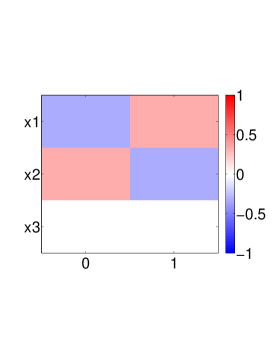
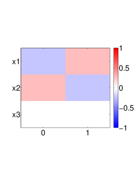

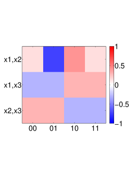
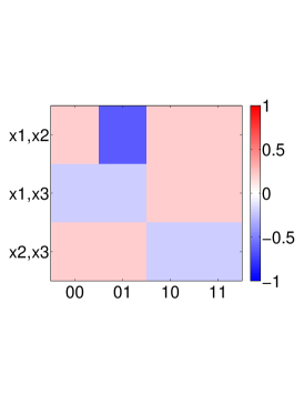
Note that the raw SVM can assign non-zero weights only to feature space dimensions (here, input variables and their pairwise conjunctions, corresponding to the quadratic kernel); all other features, here for example pairwise disjunctions, are implicitly assigned zero. The SVM assigns the biggest weight to , followed by . In contrast, for the SVM-based FIRM the most important features are followed by , which more closely resembles the truth. Note that, due to the low degree of the polynomial kernel, the SVM not capable of learning the function “by heart”; in other words, we have an underfitting situation. In fact, we have for .
The difference in FIRM and SVM-FIRM underlines that — as intended — FIRM helps to understand the learner, rather than the problem. Nevertheless a quite good approximation to the truth is found as displayed by FIRM on the true labels, for which all seven 2-tuples that lead to true output are found (black blocks) and only leads to a false value (stronger score). Values where and are combined with lead to a slightly negative value.
3.2 Gaussian Data
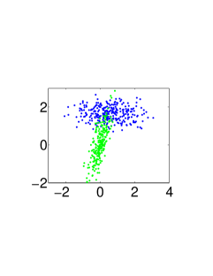
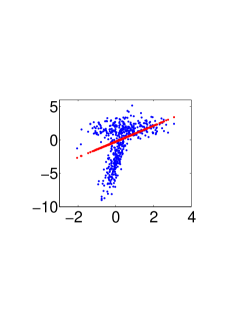
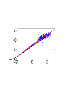
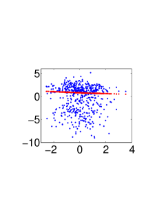
Here, we analyze a toy example to illustrate FIRM for real valued data. We consider the case of binary classification in three real-valued dimensions. The first two dimensions carry the discriminative information (cf. Figure 2a), while the third only contains random noise. The second dimension contains most discriminative information and we can use FIRM to recover this fact. To do so, we train a linear SVM classifier to obtain a classification function . Now we use the linear regression approach to model the conditional expected scores (see Figure 2b-d for the three dimensions). We observe that dimension two indeed shows the strongest slope indicating the strongest discriminative power, while the third (noise) dimension is identified as uninformative.
3.3 Sequence Data
As shown above (Section 1.2), for sequence data FIRM is essentially identical to the previously published technique POIMs [17]. To illustrate its power for sequence classification, we use a toy data set from [9]: random DNA sequences are generated, and for the positive class the sub-sequence GATTACA is planted at a random position centered around 35 (rounded normal distribution with SD=7). As biological motifs are typically not perfectly conserved, the planted consensus sequences are also mutated: for each planted motif, a single position is randomly chosen, and the incident letter replaced by a random letter (allowing for no change for of cases). An SVM with WDS kernel [6] is trained on 2500 positive and as many negative examples.
Two analyses of feature importance are presented in Figure 3: one based on the feature weights (left), the other on the feature importance (right). It is apparent that FIRM identifies the GATTACA feature as being most important at positions between 20 and 50, and it even attests significant importance to the strings with edit distance 1. The feature weighting , on the other hand, fails completely: sequences with one or two mutations receive random importance, and even the importance of the consensus GATTACA itself shows erratic behavior.
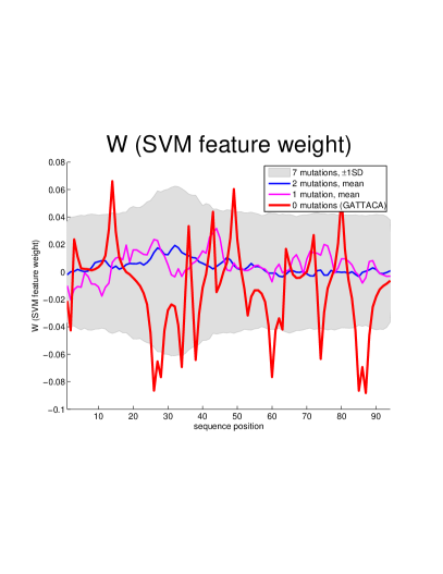
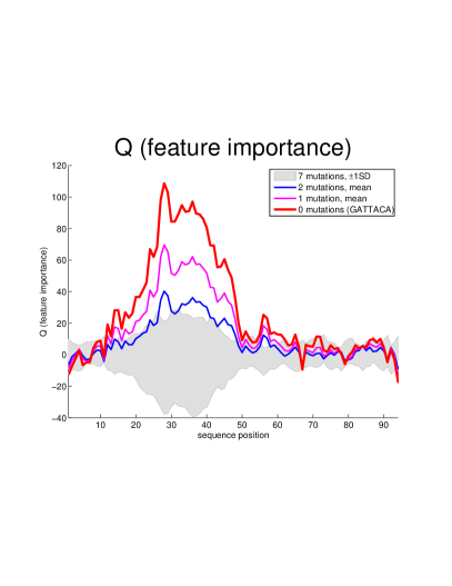
The reason is that the appearance of the exact consensus sequence is not a reliable feature, as is mostly occurs mutated. More useful features are substrings of the consensus, as they are less likely to be hit by a mutation. Consequently there is a large number of such features that are given high weight be the SVM. By taking into account the correlation of such short substrings with longer ones, in particular with GATTACA, FIRM can recover the “ideal” feature which yields the highest SVM score. Note that this “intelligent” behavior arises automatically; no more domain knowledge than the Markov distribution (and it is only -th order uniform!) is required. The practical value of POIMs for real world biological problems has been demonstrated in [17].
4 Summary and Conclusions
We propose a new measure that quantifies the relevance of features. We take up the idea underlying a recent sequence analysis method (called POIMs, [17]) — to assess the importance of substrings by their impact on the expected score — and generalize it to arbitrary continuous features. The resulting feature importance ranking measure FIRM has invariance properties that are highly desirable for a feature ranking measure. First, it is “objective”: it is invariant with respect to translation, and reasonably invariant with respect to rescaling of the features. Second, to our knowledge FIRM is the first feature ranking measure that is totally “universal”, i.e. which allows for evaluating any feature, irrespective of the features used in the primary learning machine. It also imposes no restrictions on the learning method. Most importantly, FIRM is “intelligent”: it can identify features that are not explicitly represented in the learning machine, due to the correlation structure of the feature space. This allows, for instance, to identify sequence motifs that are longer than the considered substrings, or that are not even present in a single training example.
By definition, FIRM depends on the distribution of the input features, which is in general not available. We showed that under various scenarios (e.g. binary features, normally distributed features), we can obtain approximations of FIRM that can be efficiently computed from data. In real-world scenarios, the underlying assumptions might not always be fulfilled. Nevertheless, e.g. with respect to the normal distribution, we can still interpret the derived formulas as an estimation based on first and second order statistics only.
While the quality of the computed importances does depend on the accuracy of the trained learning machine, FIRM can be used with any learning framework. It can even be used without a prior learning step, on the raw training data. Usually, feeding training labels as scores into FIRM will yield similar results as using a learned function; this is natural, as both are supposed to be highly correlated.
However, the proposed indirect procedure may improve the results due to three effects: first, it may smooth away label errors; second, it extends the set of labeled data from the sample to the entire space; and third, it allows to explicitly control and utilize distributional information, which may not be as pronounced in the training sample. A deeper understanding of such effects, and possibly their exploitation in other contexts, seems to be a rewarding field of future research.
Based on the unique combination of desirable properties of FIRM, and the empirical success of its special case for sequences, POIMs [17], we anticipate FIRM to be a valuable tool for gaining insights where alternative techniques struggle.
Acknowledgements
This work was supported in part by the FP7-ICT Programme of the European Community under the PASCAL2 Network of Excellence (ICT-216886), by the Learning and Inference Platform of the Max Planck and Fraunhofer Societies, and by the BMBF grant FKZ 01-IS07007A (ReMind). We thank Petra Philips for early phase discussion.
References
- [1] K. Bennett and O. Mangasarian. Robust linear programming discrimination of two linearly inseparable sets. Optimization Methods and Software, 1:23–34, 1992.
- [2] C. Cortes, A. Gretton, G. Lanckriet, M. Mohri, and A. Rostamizedeh. Outcome of the NIPS*08 workshop on kernel learning: Automatic selection of optimal kernels, 2008.
- [3] J. Friedman. Greedy function approximation: a gradient boosting machine. Annals of Statistics, 29:1189–1232, 2001.
- [4] A. Graf, F. Wichmann, H. H. Bülthoff, and B. Schölkopf. Classification of faces in man and machine. Neural Computation, 18:143–165, 2006.
- [5] G. R. G. Lanckriet, N. Cristianini, L. E. Ghaoui, P. Bartlett, and M. I. Jordan. Learning the kernel matrix with semidefinite programming. Journal of Machine Learning Research, 5:27–72, 2004.
- [6] G. Rätsch, S. Sonnenburg, and B. Schölkopf. RASE: Recognition of alternatively spliced exons in C. elegans. Bioinformatics, 21(Suppl. 1):i369–i377, June 2005.
- [7] J. Schäfer and K. Strimmer. A Shrinkage Approach to Large-Scale Covariance Matrix Estimation and Implications for Functional Genomics. Statistical Applications in Genetics and Molecular Biology, 4(1):32, 2005.
- [8] B. Schölkopf and A. J. Smola. Learning with Kernels. Cambridge, MIT Press, 2002.
- [9] S. Sonnenburg, G. Rätsch, and C. Schäfer. Learning interpretable SVMs for biological sequence classification. In RECOMB 2005, LNBI 3500, pages 389–407. Springer, 2005.
- [10] S. Sonnenburg, G. Rätsch, C. Schäfer, and B. Schölkopf. Large Scale Multiple Kernel Learning. Journal of Machine Learning Research, 7:1531–1565, July 2006.
- [11] C. Strobl, A. Boulesteix, T. Kneib, T. Augustin, and A. Zeileis. Conditional variable importance for random forests. BMC Bioinformatics, 9(1):307, 2008.
- [12] C. Strobl, A. Boulesteix, A. Zeileis, and T. Hothorn. Bias in random forest variable importance measures: Illustrations, sources and a solution. BMC bioinformatics, 8(1):25, 2007.
- [13] R. Tibshirani. Regression Shrinkage and Selection via the Lasso. Journal of the Royal Statistical Society, Series B, 58(1):267–288, 1996.
- [14] B. Üstün, W. J. Melssen, and L. M. Buydens. Visualisation and interpretation of support vector regression models. Analytica Chimica Acta, 595(1-2):299–309, 2007.
- [15] M. van der Laan. Statistical inference for variable importance. The International Journal of Biostatistics, 2(1):1008, 2006.
- [16] A. Zien, P. Philips, and S. Sonnenburg. Computing Positional Oligomer Importance Matrices (POIMs). Res. Report; Electronic Publ. 2, Fraunhofer FIRST, Dec. 2007.
- [17] A. Zien, S. Sonnenburg, P. Philips, and G. Rätsch. POIMS: Positional Oligomer Importance Matrices – Understanding Support Vector Machine Based Signal Detectors. In Proceedings of the 16th International Conference on Intelligent Systems for Molecular Biology, 2008.