Thermal breakage of a discrete one-dimensional string

Abstract

We study the thermal breakage of a discrete one-dimensional string, with open and fixed ends, in the heavily damped regime. Basing our analysis on the multidimensional Kramers escape theory, we are able to make analytical predictions on the mean breakage rate, and on the breakage propensity with respect to the breakage location on the string. We then support our predictions with numerical simulations.

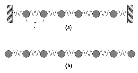
Recently, there is much discussion on the possibility of exploiting biopolymers as functional materials Sarikaya et al. (2003); Zhang (2003); Hartgerink et al. (2001); Han et al. (2007). To achieve this goal, the stabilities of such materials have to be thoroughly investigated. Furthermore, the facts that the biopolymers are necessarily finite and consist of discrete parts, such as individual peptides in an amyloid fibril Zhang (2003), have to be taken into consideration. As a step towards this direction, we study here a toy model for the breakage of a discrete one-dimensional string under thermal fluctuations, in both fixed-ended and open-ended configurations (c.f. Fig. 1). This problem has been studied previously by numerical simulations Welland et al. (1992); Oliveira and Taylor (1994); Bolton et al. (1995) and theoretically with phenomenological assumptions on the effect of friction on the collective modes Sebastian and Puthur (1999); Puthur and Sebastian (2002). Multi-dimensional Kramers escape theory has also been applied to the study of breakage in a one-dimensional ring Sain et al. (2006). The energy profile for the bonds in the string is usually modeled by a quadratic potential at the minimum energy region, and by an inverted quadratic potential at the breakage point. Here, we employ a simplified model where all bonds are assumed to be Hookian up to the breakage point. This model has the virtue of rendering the theoretical analysis asymptotically exact as temperature goes to zero. By studying in detail the energy dependency on the collective modes, we are able to employ the multidimensional Kramers escape theory to predict the breakage rate and the breakage propensity with respect to the breakage location. These predictions are then verified by numerical simulations.

.1 String with fixed ends

We consider the dynamics of a one-dimensional string modeled as a collection of $M$ masses connected by springs with identical spring constant $\kappa$. We also assume that we are in the heavily damped regime, i.e., the inertia terms are ignored, which is reasonable for many biopolymers in typical experimental conditions Sneppen and Zocchi (2005). We assume that the beads in the string are initially at the minimal energy configuration, i.e., each consecutive pair of beads is separated by a unit distance. Denoting the positional deviation of the $n$-th bead from the initial configuration by $x_{n}$, the equations of motion under thermal perturbation are of the form:

$$\frac{{\rm d}\mathbf{x}}{{\rm d}t}=-\frac{\kappa}{\zeta}A\mathbf{x}+\mathbf{g}$$ (1)

where $\zeta$ is the damping coefficient and $\mathbf{g}$ is a Gaussian noise such that

$$\langle\mathbf{g}\rangle = {\bf 0}$$ (2)

$$\langle g_{m}(t)g_{n}(t^{\prime})\rangle = \frac{2k_{B}T}{\zeta}\delta_{mn}\delta(t-t^{\prime})\ ,$$

and

$$A=\left[\begin{array}[]{rrrrr}2&-1&0&\cdots&0\\ -1&2&-1&\cdots&0\\ \vdots&&\ddots&&\vdots\\ 0&\cdots&0&-1&2\end{array}\right]\ ,$$ (3)

i.e., $A_{nn}=2$ and $A_{n+1,n}=A_{n,n+1}=-1$.

Figure 1: (a) A 1D mass-spring system with fixed ends. (b) A 1D mass-spring system with open ends. In both cases, the separation between the beads are assumed to be of unit length.

As $A$ is symmetric, it is diagonalizable by a set of orthonormal vectors. Let $D$ be the diagonal matrix such that $VDV^{\dagger}=A$ where $V$ is the corresponding orthogonal matrix, we have

$$\frac{{\rm d}\mathbf{p}}{{\rm d}t}=-\frac{\kappa}{\zeta}D\mathbf{p}+\mathbf{g}$$ (4)

where $\mathbf{p}=V^{\dagger}\mathbf{x}$ and the thermal perturbation term $\mathbf{g}$ remains the same since $V$ is an orthogonal matrix. The diagonal elements of $D$ are

$$\lambda_{s}=2\left[1-\cos\frac{\pi s}{M+1}\right]$$ (5)

and the entries in $V$ are:

$$V_{ns}=C\sin\frac{\pi sn}{M+1}\ .$$ (6)

In the above equation, $C=\sqrt{2/(M+1)}$ is the normalization factor so that $\sum_{n}V_{ns}^{2}=1$ for all $s$ (c.f. Appendix A.1).

The extension/contraction of the $n$-th spring (designating the spring before the $n$-th bead) is given by:

$$e_{1} = [V\mathbf{p}]_{1}$$ (7)

$$e_{n} = [V\mathbf{p}]_{n}-[V\mathbf{p}]_{n-1}$$ (8)

$$e_{M+1} = [V\mathbf{p}]_{M}-[V\mathbf{p}]_{M-1}\ ,$$ (9)

or in matrix notation,

$$\mathbf{e}=W\mathbf{p}$$ (10)

where $W$ is a matrix of dimension $(M+1)\times M$ such that

$$W_{1s} = V_{1s}$$ (11)

$$W_{ns} = V_{ns}-V_{n-1,s}\ \ \ ,\ \ \ 1<n\leq M$$

$$W_{M+1,s} = V_{M,s}\ .$$

We are interested in the Mean First Breakage Time (MFBT) defined as:

$$\tau=\inf_{t}\Big{\{}t>0\ \Big{|}\ \max_{n}\{|e_{n}(t)|\}>b\Big{\}}\ .$$ (12)

In physical terms, we are to find the average waiting time before any of the $e_{n}$ is extended or contracted by an amount $b$ where $b<1$ . The above problem is equivalent to a multi-dimensional Kramers escape problem Langer (1969); Hanggi et al. (1990), and we will employ the formalism developed in Matkowsky and Schuss (1977) for our analysis.

In terms of the normal modes $\{p\}$, the total energy corresponding to the entire string is

$$U(\mathbf{p})=\frac{\kappa}{2}\sum_{s}\lambda_{s}p_{s}^{2}\ ,$$ (13)

and the exit boundaries are defined by:

$$\sum_{s}W_{ns}p_{s}=\pm b\ \ \ ,\ \ \ {\rm for\ }1\leq n\leq M+1\ .$$ (14)

Our first task is to find the exit routes with the minimal energy. To do so, we employ the Lagrange multiplier method to minimize the following quantity with respect to $\mathbf{p}$:

$$U(\mathbf{p})+z_{n}\left(\sum_{s}W_{ns}p_{s}\pm b\right)\ \ \ ,\ \ \ {\rm for\ }1\leq n\leq M+1$$ (15)

where $z_{n}$ is the corresponding Lagrange multiplier. The solution to this minimization problem is that for each $n$, there are two minimizing vectors, $\hat{\bf p}^{(n)+}$ and $\hat{\bf p}^{(n)-}$, of the forms:

$$\hat{p}_{s}^{(n)\pm}=\pm\frac{W_{ns}b}{\lambda_{s}}\left(\sum_{s}\frac{W_{ns}^{2}}{\lambda_{s}}\right)^{-1}\ ,$$ (16)

such that the corresponding energy is:

$$U(\hat{\bf p}^{(n)\pm})=\frac{\kappa b^{2}}{2}\left(\sum_{s}\frac{W_{ns}^{2}}{\lambda_{s}}\right)^{-1}\ .$$ (17)

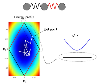
Figure 2: (Color online) Consider the case of having three beads connected by one black and one red spring. The energy profile in the $p$-space is depicted in the surface plot in the lower-left figure. Breakages of the black (red) spring correspond to the black (red) boundaries on the energy plot. A possible trajectory that leads to breaking the black spring is schematically depicted in white. The energy profile at the upper-right exit boundary is depicted in the lower-right figure. The MFBT is partly determined by the curvature of the potential energy at the exit point (c.f. Eq. (21)).

Since (c.f. Appendix A.2)

$$\sum_{s}\frac{W_{ns}^{2}}{\lambda_{s}}=\frac{M}{M+1}\ \ \ ,\ \ \ 1\leq n\leq M+1\ ,$$ (18)

the minimal energy is the same for all $n$:

$$U(\hat{\bf p}^{(n)\pm})=\frac{\kappa b^{2}(M+1)}{2M}\ \ \ ,\ \ \ 1\leq n\leq M+1\ .$$ (19)

As a result, there are $2M+2$ exit points at the boundary that correspond to the same energy. We will denote these exit points by $\mathbf{Q}^{(k)}$:

$$Q_{s}^{(k)}=(\pm 1)^{k}\frac{W_{\lceil k/2\rceil,s}b(M+1)}{\lambda_{s}M}\ \ \ ,\ \ \ 1\leq k\leq 2M+2\ .$$ (20)

In Fig. 2, we depict the energy profile and the corresponding exit points for the case of a three-bead system.

With the formalism developed in Matkowsky and Schuss (1977), in the asymptotic limit of $\kappa\rightarrow\infty$ (or equivalently, $k_{B}T\rightarrow 0$), the MFBT can be expressed exactly as:

$$\tau=\frac{\zeta\sqrt{2\pi k_{B}T}\ \exp\left[\frac{(M+1)\kappa b^{2}}{2Mk_{B}T}\right]}{\phi_{0}^{1/2}\sum_{k=1}^{2M+2}\phi_{\bar{k}}^{-1/2}|\kappa D\mathbf{Q}^{(k)}|}$$ (21)

where

$$\phi_{0} = \det\left.\frac{\partial^{2}U}{\partial p_{r}\partial p_{s}}\right|_{\mathbf{p}={\bf 0}}=\kappa^{M}\prod_{s}\lambda_{s}$$ (22)

$$\phi_{\bar{k}} = \det\left.\frac{\partial^{2}U}{\partial\hat{p}_{r}\partial\hat{p}_{s}}\right|_{\mathbf{p}=\mathbf{Q}^{(k)}}\ \ \ ,\ \ \ 1\leq r,s\leq M-1\ ,$$ (23)

with $\hat{p}_{r}(1\leq r\leq M-1)$ being a set of basis that are perpendicular to the direction of the $k$-th exit route, i.e., they are perpendicular to the direction $(W_{\lceil k/2\rceil,1},\ldots,W_{\lceil k/2\rceil,M})$. In other words, $\phi_{0}$ corresponds to the Hessian of the potential energy at the origin, and $\phi_{\bar{k}}$ corresponds to the Hessian of the potential energy within the hyperplane that has its normal pointing along the $k$-th exit route. Note also that physically, $|\kappa D\mathbf{Q}^{(k)}|$ corresponds to the magnitude of the potential energy’s gradient at the $k$-th exit point Matkowsky and Schuss (1977).

In Appendix A.3 (Eq. (26)) and Appendix A.5 (for Eqs (27) and (30)), we argue that

$$\left|\frac{\kappa}{\zeta}D\mathbf{Q}^{(k)}\right| = \left\{\begin{array}[]{l}\frac{(M+1)\kappa b}{\zeta M}\ \ \ ,\ \ \ k=1,2,2M+1,2M+2\\ \frac{\sqrt{2}(M+1)\kappa b}{\zeta M}\ \ \ ,\ \ \ {\rm otherwise}\end{array}\right.$$ (26)

$$\phi_{0} = \kappa^{M}(M+1)$$ (27)

$$\phi_{\bar{k}} = \left\{\begin{array}[]{l}\kappa^{M-1}M\ \ \ ,\ \ \ k=1,2,2M+1,2M+2\\ \kappa^{M-1}M/2\ \ \ ,\ \ \ {\rm otherwise}\ .\end{array}\right.$$ (30)

Substituting the above quantities to Eq. (21), we arrive at the following prediction for the MFBT:

$$\tau=\sqrt{\frac{\pi k_{B}TM}{8(M+1)}}\frac{\zeta}{\kappa^{3/2}b(M+1)}\ \exp\left[\frac{(M+1)\kappa b^{2}}{2k_{B}TM}\right]\ .$$ (31)

Fig. 3 demonstrated that the convergence of the numerical results to the analytical predictions as $\kappa$ increases.

Besides the MFBT, this formalism is also capable of predicting the propensity for breakage with respect to the location of the spring in the string. According to Eq. 5.1 in Matkowsky and Schuss (1977), the probability of breakage at the $n$-th segment is given by:

$$\Pr(n) = \frac{2\phi_{\bar{k}}^{-1/2}|\kappa D\mathbf{Q}^{(n)}/\zeta|}{\sum_{k=1}^{2M+2}\phi_{\bar{k}}^{-1/2}|\kappa D\mathbf{Q}^{(k)}/\zeta|}$$ (32)

$$= \left\{\begin{array}[]{ll}1/(2M)\ \ \ ,&n=1,M+1\\ 1/M\ \ \ ,&{\rm otherwise}\ .\end{array}\right.$$ (35)

This signifies that the breakage propensity is uniform for all springs except for the two extremal springs, which break half as frequently as the springs in the middle. Fig. 3 shows that the analytical predictions are in good agreement with simulations. Physically, the fact that the extremal springs break half as frequently may be seen from the fact that they are connected to the rigid wall on one side and so they are subjected to about half the amount of thermal fluctuations.

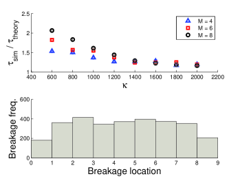
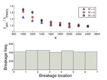
Figure 3: (Color online) Breakage events for the fixed-ended string. Upper plot: The ratios of the MFBT from simulations vs. the MFBT from theory. Each marker represents 1000 samples. The parameters are: $\zeta=10$, $k_{B}T=1$ and $b=0.1$. Lower plot: The breakage frequency with respect to the breakage location for the case of $M=8$ with the combined data from the cases of $\kappa=1600,1800,2000$.

Figure 4: (Color online) Breakage events for the opened-ended string. Upper plot: The ratios of the MFBT from simulations vs. the MFBT from theory. Each marker represents 1000 samples. The parameters are: $\zeta=10$, $k_{B}T=1$ and $b=0.1$. Lower plot: The breakage frequency with respect to the breakage location for the case of $M=8$ with the combined data from the cases of $\kappa=2000,2200,2400$.

.2 Strings with open ends

For an open-ended string as depicted in Fig. 1b, the equations of motions are governed by:

$$\frac{{\rm d}\hat{x}_{1}}{{\rm d}t} = \hat{x}_{2}-\hat{x}_{1}-1+\hat{g}_{1}$$ (36)

$$\frac{{\rm d}\hat{x}_{n}}{{\rm d}t} = \hat{x}_{n+1}-2\hat{x}_{n}+\hat{x}_{n-1}+\hat{g}_{n}\ \ \ ,\ \ \ 1<n<M$$

$$\frac{{\rm d}\hat{x}_{M}}{{\rm d}t} = \hat{x}_{M-1}-\hat{x}_{M}+1+\hat{g}_{M}$$

where $\hat{x}_{n}(t=0)=n$ and $\mathbf{g}$ is as defined in Eq. (2). We now let

$$x_{n}=\hat{x}_{n}+\frac{M-1}{2}-n+1-\frac{1}{M}\sum_{n}\hat{x}_{n}\ ,$$ (37)

i.e., these new coordinates are defined in relation to the center of mass of the string. With these transformations, the equations of motion become

$$\frac{{\rm d}\mathbf{x}}{{\rm d}t}=-\frac{\kappa}{\zeta}A\mathbf{x}+\mathbf{g}$$ (38)

where

$$A=\left[\begin{array}[]{rrrrr}1&-1&0&\cdots&0\\ -1&2&-1&\cdots&0\\ \vdots&&\ddots&&\vdots\\ 0&\cdots&0&-1&1\end{array}\right]$$ (39)

with $\mathbf{g}$ remains the same as in Eq. (2).

With $VDV^{\dagger}=A$, the diagonal elements of D are

$$\lambda_{s}=2\left[1-\cos\frac{\pi(s-1)}{M}\right]$$ (40)

and $V$ is now defined by

$$V_{ns}=C\cos\frac{\pi(n-1/2)(s-1)}{M}\ .$$ (41)

In the above equation, $C=\sqrt{2/(M+1)}$ is again the normalization factor as in the case of fixed-ended string. The proof for this statement is similar to that presented in Appendix A.1 and is thus omitted.

Note that the first normal mode, $p_{1}$, corresponds to all beads moving in unison and is thus of no interest in terms of breakage events. We will therefore omit this mode in subsequent discussion. In other words, we will only consider the set of normal modes $\{p_{s}:2\leq s\leq M\}$.

As in the previous section, we are interested in the extension/contraction given by:

$$\mathbf{e}=W\mathbf{p}$$ (42)

where $W$ is a matrix of dimension $(M-1)\times(M-1)$ such that

$$W_{ns}=V_{s,n+1}-V_{s,n}\ \ \ ,\ \ \ 1\leq n<M,\ 2\leq s\leq M\ .$$ (43)

Here, we have again

$$\sum_{s=2}^{M}\frac{W_{ns}^{2}}{\lambda_{s}}=1\ \ \ ,\ \ \ 1\leq n\leq M-1\ .$$ (44)

For an open-ended string, Eqs (26), (27) and (30) in the previous section are modified to:

$$\left|\kappa D\mathbf{Q}^{(k)}\right| = \sqrt{2}\kappa b$$ (45)

$$\phi_{0} = \kappa^{M-1}M$$ (46)

$$\phi_{\bar{k}} = \kappa^{M-2}\frac{M}{2}\ .$$ (47)

The demonstrations of the above equalities are very similar to those presented in Appendix A.3, A.4 and A.5 are therefore omitted.

Employing Eq. (21), we arrive at the following asymptotic (as $\kappa\rightarrow\infty$) prediction for the MFBT

$$\tau=\sqrt{\frac{\pi k_{B}T}{8}}\frac{\zeta}{\kappa^{3/2}b(M-1)}\ {\rm e}^{\kappa b^{2}/2k_{B}T}\ .$$ (48)

This prediction is in good agreement with simulations as shown in Fig. 4. Note also that according to this calculation, the breakage rate of an open-ended string is the same as that of a fixed-ended string when $M\gg 1$.

Since $\phi_{\bar{k}}$ and $\left|\kappa D\mathbf{Q}^{(k)}\right|$ are identical for all $k$, Eq. (32) predicts that all the springs are broken with equal frequency. In other words, contrary to the case of an fixed-ended string, we would expect a flat distribution of breakage frequencies across the string, which is indeed shown to be the case by simulations (c.f. Fig.  4). This result may be expected as, unlike in the case of a string with fixed ends, the extremal springs here are again connecting two fluctuating beads. We therefore expect that their breakage frequencies would be similar to those for the springs in the middle of the chain.

In summary, we have investigated analytically the breakage rate for an 1D string under thermal fluctuation in the heavily damped regime. Our approach is based on the theory of the multi-dimensional Kramers escape problem, and we have supported our analytical predictions with numerical simulations.

Appendix A Proofs of various identities

A.1 Claim: $C^{2}=2/(M+1)$

By definition:

$$C^{-2} = \sum_{s}\sin^{2}\frac{\pi sn}{M+1}$$ (49)

$$= \frac{1}{2}\sum_{s=1}^{M}\left(1-\cos\frac{2\pi ns}{M+1}\right)$$ (50)

$$= \frac{M+1}{2}-\frac{1}{2}\sum_{s=0}^{M}\cos\frac{2\pi ns}{M+1}$$ (51)

where the second term in Eq. (51) is zero as the negative terms cancel the positive terms exactly.

A.2 Claim: $\sum_{s}\frac{W_{ns}^{2}}{\lambda_{s}}=1$ for all $n$

For $n=1$, we have

$$\sum_{s}\frac{W_{ns}^{2}}{\lambda_{s}} = \frac{C^{2}}{2}\sum_{s=1}^{M}\frac{\sin^{2}(\pi s/(M+1))}{[1-\cos(\pi s/(M+1)]}$$ (52)

$$= \frac{C^{2}}{2}\sum_{s}[1+\cos(\pi s/(M+1)]$$ (53)

$$= \frac{M}{M+1}\ .$$ (54)

The case for $n=M$ follows similarly.

If $n$ is not 1 or $M$, $\sum_{s}\frac{W_{ns}^{2}}{\lambda_{s}}$ is by definition:

$$\frac{C^{2}}{2}\sum_{s=1}^{M}\frac{[\sin(\pi sn/(M+1))-\sin(\pi s(n-1)/(M+1))]^{2}}{1-\cos(\pi s/(M+1)}$$

$$= C^{2}\sum_{s}\frac{\cos^{2}(\pi s(2n-1)/(2M+2))\sin^{2}(\pi s/(2M+2))}{\sin^{2}(\pi s/(2M+2)}$$

$$= C^{2}\sum_{s}\cos^{2}\frac{\pi s(2n-1)}{2M+2}$$

$$= \frac{M}{M+1}+\frac{C^{2}}{2}\sum_{s}\cos\frac{\pi s(2n-1)}{M+1}$$

as the second term in the last equality is zero.

A.3 Claim: $\sum_{s}W^{2}_{ns}$ equals 1 for $n=1,M+1$ and equals 2 otherwise

Firstly we prove that $\sum_{s}W^{2}_{ns}$ is 1 for $n=1,M+1$ and is 2 otherwise. The fact that $\sum_{s}W^{2}_{ns}=1$ for $n=1,M+1$ follows immediately from Eqs 11. For $n\neq 1,M+1$, We have

$$\sum_{s}W^{2}_{ns} = C^{2}\sum_{s}\left[\sin\frac{\pi sn}{M+1}-\sin\frac{\pi s(n-1)}{M+1}\right]^{2}$$

$$= 2-2C^{2}\sum_{s}\sin\frac{\pi sn}{M+1}\sin\frac{\pi s(n-1)}{M+1}$$

$$= 2+C^{2}\sum_{s}\left[\cos\frac{\pi s(2n-1)}{M+1}-\cos\frac{\pi s}{M+1}\right]$$

$$= 2\ .$$

A.4 Computations for $\phi_{0}$

By Eq. (22),

$$\phi_{0} = \kappa^{M}\prod_{s=1}^{M}\lambda_{s}$$ (56)

$$= (2\kappa)^{M}\prod_{s=1}^{M}\left[1-\cos\frac{\pi s}{M+1}\right]$$ (57)

$$= (4\kappa)^{M}\left[\prod_{s=1}^{M}\sin\frac{\pi s}{2(M+1)}\right]^{2}$$ (58)

$$= \kappa^{M}(M+1)$$ (59)

where the last equality follows from the identity in wolfram .

A.5 Computations for $\phi_{\bar{k}}$

By rotating the basis, we have a new coordinates, $\mathbf{y}=(y_{1},\ldots,y_{M})$, such that the direction $(0,\ldots,0,1)$ corresponds to the direction that is normal to the exit boundary at the $k$-th exit point. Let us denote the orthogonal matrix that transforms from this new set of basis back to the $p$-space by $R$. In particular, we have

$$R_{sM}=\frac{W_{ks}}{\sqrt{\sum_{s}W_{ks}^{2}}}\ .$$ (60)

Note that one way to obtain the rest of the matrix elements in $R$ is to employ the Gram-Schmidt process.

In terms of this new coordinates, the potential energy is:

$$U(\mathbf{y}) = \frac{\kappa}{2}\mathbf{p}^{T}D\mathbf{p}$$ (61)

$$= \frac{\kappa}{2}\mathbf{y}^{T}R^{T}DR\mathbf{y}$$ (62)

Restricting to the first $M-1$ dimensions, $\phi_{\bar{k}}$ is defined as:

$$\phi_{\bar{k}}=\det\Big{(}[R^{T}DR]_{1\leq r,s\leq M-1}\Big{)}\ .$$ (63)

We have calculated this quantity for $M=3,4,\ldots,50$ numerically and we find that the following formula is exactly satisfied (up to machine rounding errors):

$$\phi_{\bar{k}}=\left\{\begin{array}[]{l}\kappa^{M-1}M\ \ \ ,\ \ \ k=1,2,2M+1,2M+2\\ \kappa^{M-1}M/2\ \ \ ,\ \ \ {\rm otherwise}\end{array}\right.\ .$$ (64)

Although we are not able to prove the above equality mathematically, we believe that it holds true for all $M$.

Appendix B Details of numerical simulations

Simulations performed for the dynamics of strings with fixed ends (free ends) are based on Eq. (1) with the matrix $A$ defined in Eq. (3) (Eq. (39)). Namely, the positions of the beads are updated according to the following scheme:

$$\mathbf{x}(t+\triangle t)=\mathbf{x}(t)-\frac{\kappa}{\zeta}A\mathbf{x}(t)\triangle t+\sqrt{\frac{2k_{B}T\triangle t}{\zeta}}\ \mathbf{z}(t)$$ (65)

where $\mathbf{z}(t)$ is a vector with entries given by random numbers drawn from the normal distribution with zero mean and a standard deviation of one. The simulations always start at the minimal energy configurations and are terminated when one of the springs’ lengths become more than 1.1 or smaller than 0.9. The parameters in the simulations are: $\zeta=10$, $k_{B}T=1$, and $\triangle t$ is set to be $2\times 10^{-6}$. For each set of parameters, 1000 runs are performed.

References

• Sarikaya et al. (2003) M. Sarikaya, C. Tamerler, A. K. Jen, K. Schulten, and F. Baneyx, Nat Mater 2, 577 (2003).
• Zhang (2003) S. Zhang, Nat Biotech 21, 1171 (2003).
• Hartgerink et al. (2001) J. D. Hartgerink, E. Beniash, and S. I. Stupp, Science 294, 1684 (2001).
• Han et al. (2007) T. . H. Han, J. Kim, J. . S. Park, C. . B. Park, H. Ihee, and S. . O. Kim, Advanced Materials 19, 3924 (2007).
• Welland et al. (1992) R. W. Welland, M. Shin, D. Allen, and J. B. Ketterson, Physical Review B 46, 503 (1992).
• Bolton et al. (1995) K. Bolton, S. Nordholm, and H. W. Schranz, The Journal of Physical Chemistry 99, 2477 (1995).
• Oliveira and Taylor (1994) F. A. Oliveira and P. L. Taylor, The Journal of Chemical Physics 101, 10118 (1994).
• Sebastian and Puthur (1999) K. L. Sebastian and R. Puthur, Chemical Physics Letters 304, 399 (1999).
• Puthur and Sebastian (2002) R. Puthur and K. L. Sebastian, Physical Review B 66, 024304 (2002).
• Sain et al. (2006) A. Sain, C. L. Dias, and M. Grant, Physical Review E 74, 046111 (2006).
• Sneppen and Zocchi (2005) K. Sneppen and G. Zocchi, Physics in Molecular Biology (Cambridge University Press, Cambridge, 2005).
• Hanggi et al. (1990) P. Hanggi, P. Talkner, and M. Borkovec, Reviews of Modern Physics 62, 251 (1990).
• Langer (1969) J. Langer, Annals of Physics 54, 258 (1969).
• Matkowsky and Schuss (1977) B. J. Matkowsky and Z. Schuss, SIAM Journal on Applied Mathematics 33, 365 (1977).
• (15) See http://functions.wolfram.com/01.06.24.0001.01.