Two-Dimensional ARMA Modeling for Breast Cancer Detection and Classification

Abstract

We propose a new model-based computer-aided diagnosis (CAD) system for tumor detection and classification (cancerous v.s. benign) in breast images. Specifically, we show that (x-ray, ultrasound and MRI) images can be accurately modeled by two-dimensional autoregressive-moving average (ARMA) random fields. We derive a two-stage Yule-Walker Least-Squares estimates of the model parameters, which are subsequently used as the basis for statistical inference and biophysical interpretation of the breast image. We use a k-means classifier to segment the breast image into three regions: healthy tissue, benign tumor, and cancerous tumor. Our simulation results on ultrasound breast images illustrate the power of the proposed approach.

Index Terms—  Breast cancer, two-dimensional ARMA models, k-means algorithm.

1 Introduction

Breast cancer continues to be a significant public health problem in the United States: It is the second leading cause of female mortality, and, disturbingly, one out of eight women in the United States will be diagnosed with breast cancer in her life time. Until the cause of this disease is fully understood, early detection remains the only hope to improve breast cancer prognosis and treatment. Breast cancer screening modalities are mainly based on clinical examination, mammography, ultrasound imaging, magnetic resonance imaging (MRI), and core biopsy. Mammography (breast x-ray imaging) is by far the fastest and cheapest screening test for breast cancer. Unfortunately, it is also among the most difficult of radiological images to interpret: mammograms are of low contrast, and features indicative of breast disease are often very small. Many studies have shown that ultrasound and MRI imaging techniques can help supplement mammography by detecting small breast cancers that may not be visible with mammography. However, these techniques often fail to determine if a detected tumor is cancerous or benign, and a biopsy may be recommended. Consequently, many unnecessary biopsies are often undertaken due to the high false positive rate.

Computer aided diagnosis (CAD) paradigms have recently received great attention for lesion detection and discrimination in X-ray and ultrasound breast mammograms [1, 2, 3, 4]. The large amount of negative biopsies encountered in clinical practice could be reduced if a computer system was available to help the radiologists screen breast images. Broadly, the CAD systems proposed in the literature can be grouped into four major categories: geometrical [1], artificial intelligence [2], pyramidal (or multiresolution) [3], and model-based techniques [4], [5]. Geometrical methods employ morphological and other segmentation techniques to extract small specks of calcium known as microcalcifications from breast images [1]. However, this procedure usually requires a priori knowledge of the tumor pattern characteristics. Moreover, these techniques also tend to rely on many stages of heuristics attempting to eliminate false positives. Artificial intelligence techniques include neural networks and fuzzy logic methods. The performance of these systems is tied to the architecture of the network and the number of training data. Breast cancer is a heterogeneous disease which includes several subtypes with distinct prognosis. In particular, the variability associated with the appearances of the breast cancer, ranging from relative uniformity to complex patterns of bright streaks and blobs [2], makes the ANN require a large training data set to ensure a certain level of reliability. Pyramidal or multiresolution techniques refer mainly to the wavelet transform [3], which can be seen from a signal decomposition view point. Specifically, a signal is decomposed onto a set of the basis wavelet functions. A very appealing feature of the wavelet analysis is that it provides a uniform resolution for all the scales. Limited by the size of the basic wavelet function, the downside of the uniform resolution is uniformly poor resolution. Model-based methods include linear, non-linear and finite-element methods to build an accurate model of the breast [4], [5]. The model is subsequently used for image matching, detection, and classification [5]. The accuracy of the results are tied to the accuracy of the considered model.

In this work, we propose a new model-based CAD system for tumor detection and classification. We show that (x-ray, ultrasound, and MRI) breast images can be accurately modeled by two-dimensional autoregressive moving average (ARMA) random fields. The model parameters, being the fingerprints of the image, serve as the basis for statistical inference and biophysical interpretation of the breast image. ARMA models are parametric representations of wide-sense stationary (WSS) processes with rational spectra. The Wold decomposition theorem states that any WSS process can be decomposed as the sum of a regular process, which spectrum is continuous, and a predictable process, which spectrum consists of impulses. Since rational spectra form a dense set in the class of continuous spectra, the ARMA model renders accurately the regular part of the WSS process. It is, therefore, surprising that very few researchers have attempted to derive a general ARMA representation of the breast, and use it for tumor detection and classification. In [5], the authors use a one-dimensional fractional differencing autoregressive moving average (FARMA) process to model the ultrasound RF echo reflected from the breast tissue. However, by considering separate scan lines, they do not take into account the two-dimensional spatial correlation between the pixels in the image. In [6], an autoregressive (AR) model is considered for improving the contrast of breast cancer lesions in ultrasound images. ARMA models, however, provide a more accurate model of a homogeneous random field than an AR model. As in the 1D case, the 2D ARMA parameter estimation problem is much more difficult than its 2D AR counterpart, due to the non-linearity in estimating the 2D moving average (MA) parameters.

This paper is organized as follows: In Section 2, we define the 2D ARMA representation of the breast image, and derive a Yule-Walker Least squares estimates of its parameters [7]. In Section 3, we use the estimated ARMA coefficients as vector features for the k-means classifier. The simulation results, for ultrasound breast images showing cancerous and benign tumors, are shown in Section 4. Finally, in Section 5, we summarize our contribution and provide concluding remarks.

2 2D ARMA Modeling

We represent the breast image as a 2D random field $\{x[n,m],\\ (n,m)\in\mathbb{Z}^{2}\}$. We define a total order on the discrete lattice as follows

$$(i,j)\leq(s,t)\Longleftrightarrow i\leq s~{}~{}\text{and}~{}~{}j\leq t.$$ (1)

The 2D ARMA($p_{1},p_{2},q_{1},q_{2}$) model is defined for the $N_{1}\times N_{2}$ image $I=\{x[n,m]:0\leq n\leq N_{1}-1,0\leq m\leq N_{2}-1\}$ by the following difference equation

$$x[n,m]+\mathop{\sum_{i=0}^{p_{1}}\sum_{j=0}^{p_{2}}}_{(i,j)\neq(0,0)}a_{ij}x[n-i,m-j]=$$

$$w[n,m]+\mathop{\sum_{i=0}^{q_{1}}\sum_{j=0}^{q_{2}}}_{{(i,j)\neq(0,0)}}b_{ij}w[n-i,m-j],$$ (2)

where $\{w[n,m]\}$ is a white noise field with variance $\sigma^{2}$, and the coefficients $\{a_{ij}\},\{b_{ij}\}$ are the parameters of the model. From Eq. (2), the image $\{x[n,m]\}$ can be viewed as the output of the linear time-invariant causal system $H(z_{1},z_{2})$ excited by a white noise input, where

$$H(z_{1},z_{2})=\frac{B(z_{1},z_{2})}{A(z_{1},z_{2})}=\frac{\sum_{i=0}^{q_{1}}\sum_{j=0}^{q_{2}}b_{ij}~{}z_{1}^{-i}z_{2}^{-j}}{\sum_{i=0}^{p_{1}}\sum_{j=0}^{p_{2}}a_{ij}~{}z_{1}^{-i}z_{2}^{-j}},$$ (3)

with $a_{00}=b_{00}=1$.

2.1 Yule-Walker Least-Squares Parameter Estimation

Assume first that the noise sequence $\{w[n,m]\}$ were known. Then the problem of estimating the parameters in the ARMA model (2) would be a simple input-output system parameter estimation problem, which could be solved by several methods, the simplest of which is the least-squares (LS) method. In the LS method, we express Eq. (2) as

$$x[n,m]+\phi^{t}[n,m]\theta=w[n,m],$$ (4)

where

$$\phi^{t}[n,m] = [x[n,m-1],\cdots,x[n-p_{1},m-p_{2}],-w[n,m-1],$$

$$\cdots,-w[n-q_{1},m-q_{2}]],$$

and

$$\theta=[a_{01},\cdots,a_{p_{1}p_{2}},b_{01},\cdots,b_{q_{1}q_{2}}]^{t}.$$

Writing Eq. (4) in matrix form for $n=L+1,\cdots,N_{1}-1$, and $m=M+1,\cdots,N_{2}-1,$  for some $L>\max(p_{1},q_{1})$, and $M>\max(p_{2},q_{2})$, gives

$$\mathbf{x}+\Phi\mathbf{\theta}=\mathbf{w},$$ (5)

where

$$\mathbf{x}=[x[L+1,M+1],\cdots,x[N_{1}-1,N_{2}-1]]^{t},$$

$$\mathbf{w}=[w[L+1,M+1],\cdots,x[N_{1}-1,N_{2}-1]]^{t},$$

and $\Phi$ is displayed below.

$$\Phi=\left(\begin{array}[]{cccccc}x[L+1,M]&\cdots&x[L+1-p_{1},M+1-p_{2}]&-w[L+1,M]&\cdots&-w[L+1-q_{1},M+1-q_{2}]\\ x[L+2,M]&\cdots&x[L+2-p_{1},M+1-p_{2}]&-w[L+2,M]&\cdots&-w[L+2-q_{1},M+1-q_{2}]\\ \vdots&&\vdots&\vdots&&\vdots\\ x[N_{1}-1,N_{2}-2]&\cdots&x[N_{1}-1-p_{1},N_{2}-1-p_{2}]&-w[N_{1}-1,N_{2}-2]&\cdots&-w[N_{1}-1-q_{1},N_{2}-1-q_{2}]\\ \end{array}\right).$$

Assume we know $\Phi$, then we can obtain a least-squares estimate of the parameter vector $\theta$ in Eq. (5) as

$$\hat{\theta}=-(\Phi^{t}\Phi)^{-1}\Phi^{t}\mathbf{x}.$$ (6)

Observe that the input model noise $\{w[n,m]\}$ in $\Phi$ is unknown. Nevertheless, it can be estimated by considering the noise process $w[n,m]$ as the output of the linear filter $\frac{1}{H(z_{1},z_{2})}=\frac{A(z_{1},z_{2})}{B(z_{1},z_{2})}$ with input $x[n,m]$. From Nirenberg’s proof of the division theorem in multi-dimensional spaces [8], we can write the inverse ARMA filter $\frac{A(z_{1},z_{2})}{B(z_{1},z_{2})}$ as the infinite order AR filter $\sum_{i=0}^{\infty}\sum_{j=0}^{\infty}\alpha_{ij}z_{1}^{-i}z_{2}^{-j}$. In the time domain, we obtain

$$x[n,m]+\mathop{\sum_{i=0}^{\infty}\sum_{j=0}^{\infty}}_{(i,j)\neq(0,0)}\alpha_{ij}~{}x[n-i,m-j]=w[n,m].$$ (7)

Therefore, we can estimate $\{w[n,m]\}$ by first estimating the AR parameters $\{\alpha_{ij}\}$ and next obtaining $\{w[n,m]\}$ by filtering $\{x[n,m]\}$ as in Eq. (7). Since we cannot estimate an infinite number of (independent) parameters from a finite number of samples, we approximate the finite AR model by one of finite order, say $(K_{1},K_{2})$. The parameters in the truncated AR model can be estimated by using a 2D extension of the Yule-Walker equations as follows

$$r[k,l]+\mathop{\sum_{i=0}^{K_{1}}\sum_{j=0}^{K_{2}}}_{(i,j)\neq(0,0)}\alpha_{ij}r[k-i,l-j]=\sigma^{2}\delta[k,l],$$ (8)

where $\{r[k,l]\}$ are the autocorrelation values of the field $\{x[n,m]\}$, computed as follows

$$r[k,l]=\frac{1}{(N-k)(M-l)}\sum_{i=1}^{N-k}\sum_{j=1}^{M-l}x[i,j]x[i+k,j+l],$$

$$r[-k,-l]=r[k,l],~{}\text{for}~{}(k,l)\geq(0,0)$$

$$r[k,-l]=r[-k,l],~{}\text{for}~{}(k,l)\geq(1,1),$$ (9)

and $\delta[k,l]$ is the 2D Kronecker delta function. Equation (8) is a system of linear equations that can be written in matrix form and solved for the coefficients $\alpha_{ij}$. Finally, the Yule-Walker Least-Squares algorithm is summarized below

1. Estimate the parameters $\{\alpha_{ij}\}$ in an AR($K_{1},K_{2}$) model of $x[n,m]$ by the YW method in (8). Obtain an estimate of the noise field $\{w[n,m]\}$ by

   $$\hat{w}[n,m]=x[n,m]+\mathop{\sum_{i=0}^{K_{1}}\sum_{j=0}^{K_{2}}}_{(i,j)\neq(0,0)}\hat{\alpha}_{ij}x[n-i,m-j],$$

   for $n=K_{1}+1,\cdots,N_{1}$, and $m=K_{2}+1,\cdots,N_{2}$.

2. Replace the $w[n,m]$ by $\hat{w}[n,m]$ computed in Step 1. Obtain $\hat{\theta}$ in (6) with $L=K_{1}+q_{1}$, and $M=K_{2}+q_{2}$.

3 Tumor Detection and Classification

The estimated ARMA parameters, $\{a_{ij}\},\{b_{ij}\}$, are used as a basis for inference about the presence of a tumor and its nature: benign or cancerous. We use the k-means algorithm to segment the breast image into 3 classes: healthy tissue, benign tumor and cancerous tumor. Our method consists of representing each pixel in the image by an ARMA model whose parameters are estimated by using an appropriate neighborhood for the pixel. We make the assumption that all pixels in the considered neighborhood belong to the same class, and hence, for computational efficiency, we replace the entire neighborhood by the vector value of the estimated ARMA parameters. This procedure is repeated for the entire image, creating a new block by block vector-valued image, which will be the input to the k-means classifier.

                                          (a)                               (b)                               (c)
                                          (d)                               (e)                               (f)

Fig. 1: ARMA modeling and segmentation of ultrasound breast images: (a) cancerous ultrasound image; (b) ARMA representation of (a); (c) Segmentation of (a); (d) benign tumor ultrasound image; (e) ARMA representation of (d); (f) Segmentation of (d).

4 Simulations

Although the proposed algorithm is independent of the imaging modality of the breast, we perform our simulations on ultrasound images, collected from the Radiology department, College of Medicine at the University of Illinois at Chicago. Our database of cancerous images show intraductal carcinoma, which is the most common type of breast cancer in women. Intraductal carcinoma is usually discovered through a mammogram or an ultrasound as microcalcifications. Our benign tumor images show the Fibroadenoma of the breast, which is a benign fibroepithelial tumor characterized by proliferation of both glandular and stromal elements.

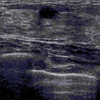
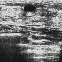
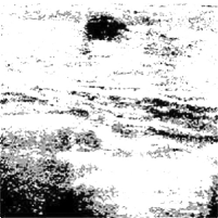
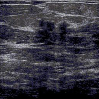
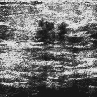
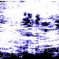
We estimate the ARMA parameters using a window of size $16\times 16$. The choice of the window size presents an inherent trade-off between the accuracy of the representation and the accuracy of the classification. A large window size would lead a better representation of the ARMA model, but might include pixels from different classes. We found that for $256\times 256$ images, a $16\times 16$ window size leads to a good segmentation performance. Figure 1 shows a cancerous image and a benign tumor image. Their ARMA representations are displayed in Figs. 1(b) and 1(e), respectively. It is visually clear that the ARMA model accurately represents both ultrasound images. Figures 1(c) and 1(f) show the segmentation outputs of the cancerous and benign tumor images, respectively. We can observe clear delineations of the tumors from the healthy tissues in both cases. Using the University of Illinois at Chicago’s database of ultrasound breast images, our method yields an accuracy (number of images correctly classified divided by the total number of images) of 82% (see Table 1).

Table 1: Detection accuracy for the University of Illinois at Chicago’s database of ultrasound breast images

Accuracy

$82\%$

5 Conclusion

We showed that breast images can be accurately represented by 2D ARMA models. Furthermore, the parameters of the model can be thought of as the fingerprints of the image, which are exploited for tumor detection and classification. Our simulation results show that, based on the estimated ARMA parameters as feature vectors, the classic k-means algorithm genuinely segment the breast images into healthy tissue, cancerous tumor and benign tumor. The end product is a computer-aided diagnosis (CAD) system that clinically portends an accurate prognosis of breast cancer.

6 Acknowledgements

The authors want to thank Dr. Karen Lin Xie from the Radiology department at the University of Illinois at Chicago for providing the ultrasound breast images.

References

- [1] N.H. Eltonsy, G.D. Tourassi, and A.S. Elmaghraby, “A concentric morphology model for the detection of masses in mammography,” IEEE Transactions on Medical Imaging, vol. 26, no. 6, pp. 880–889, 2007.
- [2] L. Wei, Y. Yang, R.M. Nishikawa, and Y. Jiang;, “A study on several machine-learning methods for classification of malignant and benign clustered microcalcifications,” IEEE Transactions on Medical Imaging, vol. 24, no. 3, pp. 371–380, March 2005.
- [3] A. Mencattini, M. Salmeri, R. Lojacono, M. Frigerio, and F. Caselli, “Mammographic images enhancement and denoising for breast cancer detection using dyadic wavelet processing,” IEEE Transactions on Instrumentation and Measurement, vol. 57, no. 7, pp. 1422–1430, July 2008.
- [4] P. Pathmanathan, D.J. Gavaghan, J.P. Whiteley, S.J. Chapman, and J.M. Brady, “Predicting tumor location by modeling the deformation of the breast,” IEEE Transactions on Biomedical Engineering, vol. 55, no. 10, pp. 2471–2480, October 2008.
- [5] B. Alacam, B. Yazici, N. Bilgutay, F. Forsberg, and C. Piccoli, “Breast tissue characterization using FARMA modeling of ultrasonic RF echo,” Ultrasound in Medicine and Biology, vol. 30, no. 10, pp. 1397–1407, October 2004.
- [6] E. von Lavante and J. A. Noble, Improving the Contrast of Breast Cancer Masses in Ultrasound Using an Autoregressive Model, vol. 4791 of Lecture Notes in Computer Science, Springer, Berlin/Heidelberg, 2007.
- [7] P. Stoica and R. L. Moses, Spectral Analysis of Signals, Prentice Hall, 2005.
- [8] L. Nirenberg, “A proof of the malgrange preparation theorem,” Springer Lecture Notes in Math, vol. 192, pp. 97–105, 1971.