A Variance Reduction Method
for Parametrized Stochastic Differential Equations
using the Reduced Basis Paradigm

Sébastien Boyaval CERMICS, Ecole des Ponts ParisTech (Université Paris-Est), Cité Descartes, 77455 Marne-la-Vallée Cedex 2, France,  and  MICMAC team-project, INRIA, Domaine de Voluceau, BP. 105 Rocquencourt 78153 Le Chesnay Cedex, France.    Tony Lelièvre\ {}^{\dagger}
Abstract

In this work, we develop a reduced-basis approach for the efficient computation of parametrized expected values, for a large number of parameter values, using the control variate method to reduce the variance. Two algorithms are proposed to compute online, through a cheap reduced-basis approximation, the control variates for the computation of a large number of expectations of a functional of a parametrized Itô stochastic process (solution to a parametrized stochastic differential equation). For each algorithm, a reduced basis of control variates is pre-computed offline, following a so-called greedy procedure, which minimizes the variance among a trial sample of the output parametrized expectations. Numerical results in situations relevant to practical applications (calibration of volatility in option pricing, and parameter-driven evolution of a vector field following a Langevin equation from kinetic theory) illustrate the efficiency of the method.

keywords:
Variance Reduction, Stochastic Differential Equations, Reduced-Basis Methods. AMS subject classifications. 60H10, 65C05.
footnotetext: Corresponding author: S. Boyaval.
Email address: boyaval@cermics.enpc.fr
URL home page: http://cermics.enpc.fr/similar-to\simboyaval/home.html
Tel: + 33 1 64 15 35 79 - Fax: + 33 1 64 15 35 86

1 Introduction

This article develops a general variance reduction method for the many-query context where a large number of Monte-Carlo estimations of the expectation 𝔼(Zλ)𝔼superscript𝑍𝜆\mathbb{E}\left(Z^{\lambda}\right) of a functional

Zλ=gλ(XTλ)0Tfλ(s,Xsλ)𝑑ssuperscript𝑍𝜆superscript𝑔𝜆superscriptsubscript𝑋𝑇𝜆superscriptsubscript0𝑇superscript𝑓𝜆𝑠superscriptsubscript𝑋𝑠𝜆differential-d𝑠Z^{\lambda}=g^{\lambda}(X_{T}^{\lambda})-\int_{0}^{T}f^{\lambda}(s,X_{s}^{\lambda})\,ds (1.1)

of the solutions (Xtλ,t[0,T])superscriptsubscript𝑋𝑡𝜆𝑡0𝑇\left(X_{t}^{\lambda},t\in[0,T]\right) to the stochastic differential equations (SDEs):

Xtλ=x+0tbλ(s,Xsλ)𝑑s+0tσλ(s,Xsλ)𝑑Bssuperscriptsubscript𝑋𝑡𝜆𝑥superscriptsubscript0𝑡superscript𝑏𝜆𝑠superscriptsubscript𝑋𝑠𝜆differential-d𝑠superscriptsubscript0𝑡superscript𝜎𝜆𝑠superscriptsubscript𝑋𝑠𝜆differential-dsubscript𝐵𝑠X_{t}^{\lambda}=x+\int_{0}^{t}b^{\lambda}(s,X_{s}^{\lambda})\,ds+\int_{0}^{t}\sigma^{\lambda}(s,X_{s}^{\lambda})dB_{s} (1.2)

parametrized by λΛ𝜆Λ\lambda\in\Lambda have to be computed for many values of the parameter λ𝜆\lambda.

Such many-query contexts are encountered in finance for instance, where pricing options often necessitates to compute the price 𝔼(Zλ)𝔼superscript𝑍𝜆\mathbb{E}\left(Z^{\lambda}\right) of an option with spot price Xtλsuperscriptsubscript𝑋𝑡𝜆X_{t}^{\lambda} at time t𝑡t in order to calibrate the local volatility σλsuperscript𝜎𝜆\sigma^{\lambda} as a function of a (multi-dimensional) parameter λ𝜆\lambda (that is minimize over λ𝜆\lambda, after many iterations of some optimization algorithm, the difference between observed statistical data with the model prediction). Another context for application is molecular simulation, for instance micro-macro models in rheology, where the mechanical properties of a flowing viscoelastic fluid are determined from the coupled evolution of a non-Newtonian stress tensor field 𝔼(Zλ)𝔼superscript𝑍𝜆\mathbb{E}\left(Z^{\lambda}\right) due to the presence of many polymers with configuration Xtλsuperscriptsubscript𝑋𝑡𝜆X_{t}^{\lambda} in the fluid with instantaneous velocity gradient field λ𝜆\lambda. Typically, segregated numerical schemes are used: compute Xtλsuperscriptsubscript𝑋𝑡𝜆X_{t}^{\lambda} for a fixed field λ𝜆\lambda, and then compute λ𝜆\lambda for a fixed field 𝔼(Zλ)𝔼superscript𝑍𝜆\mathbb{E}\left(Z^{\lambda}\right). Such tasks are known to be computationally demanding and the use of different variance reduction techniques to alleviate the cost of Monte-Carlo computations in those fields is very common (see [2, 19, 22, 3] for instance).

In the following, we focus on one particular variance reduction strategy termed the control variate method [10, 21, 20]. More precisely, we propose new approaches in the context of the computation of 𝔼(Zλ)𝔼superscript𝑍𝜆\mathbb{E}\left(Z^{\lambda}\right) for a large number of parameter values λ𝜆\lambda, with the control variate method. In these approaches, the control variates are computed through a reduced-basis method whose principle is related to the reduced-basis method [17, 18, 23, 4, 5] previously developed to efficiently solve parametrized partial differential equations (PDEs). Following the reduced-basis paradigm, a small-dimensional vector basis is first built offline to span a good linear approximation space for a large trial sample of the λ𝜆\lambda-parametrized control variates, and then used online to compute control variates at any parameter value. The offline computations are typically expensive, but done once for all. Consequently, it is expected that the online computations (namely, approximations of 𝔼(Zλ)𝔼superscript𝑍𝜆\mathbb{E}\left(Z^{\lambda}\right) for many values of λ𝜆\lambda) are very cheap, using the small-dimensional vector basis built offline for efficiently computing control variates online. Of course, such reduced-basis approaches can only be efficient insofar as:

  1. 1.

    online computations (of one output 𝔼(Zλ)𝔼superscript𝑍𝜆\mathbb{E}\left(Z^{\lambda}\right) for one parameter value λ𝜆\lambda) are significantly cheaper using the reduced-basis approach than without, and

  2. 2.

    the amount of outputs 𝔼(Zλ)𝔼superscript𝑍𝜆\mathbb{E}\left(Z^{\lambda}\right) to be computed online (for many different parameter values λ𝜆\lambda) is sufficient to compensate for the (expensive) offline computations (needed to build the reduced basis).

In this work, we will study numerically how the variance is reduced in two examples using control variates built with two different approaches.

The usual reduced-basis approach for parametrized PDEs also traditionally focuses on the certification of the reduction (in the parametrized solution manifold) by estimating a posteriori the error between approximations obtained before/after reduction for some output which is a functional of the PDE solution. Our reduced-basis approach for the parametrized control variate method can also be cast into a goal-oriented framework similar to the traditional reduced basis method. One can take the expectation 𝔼(Zλ)𝔼superscript𝑍𝜆\mathbb{E}\left(Z^{\lambda}\right) as the reduced-basis output, while the empirically estimated variance VarM(Zλ)subscriptVarMsuperscript𝑍𝜆{\rm Var_{M}}\left(Z^{\lambda}\right) serves as a computable (statistical) error indicator for the Monte-Carlo approximations EM(Zλ)subscriptEMsuperscript𝑍𝜆{\rm E_{M}}\left(Z^{\lambda}\right) of 𝔼(Zλ)𝔼superscript𝑍𝜆\mathbb{E}\left(Z^{\lambda}\right) in the limit of large M𝑀M through the Central Limit Theorem (see error bound (2.6) in Section 2.1).

In the next Section 2, the variance reduction issue and the control variate method are introduced, as well as the principles of our reduced-basis approaches for the computation of parametrized control variates. The Section 3 exposes details about the algorithms which are numerically applied to test problems in the last Section 4.

The numerical simulations show good performance of the method for the two test problems corresponding to the applications mentionned above: a scalar SDE with (multi-dimensional) parametrized diffusion (corresponding to the calibration of a local volatility in option pricing), and a vector SDE with (multi-dimensional) parametrized drift (for the parameter-driven evolution of a vector field following a Langevin equation from kinetic theory). Using the control variate method with a 202020-dimensional reduced basis of (precomputed) control variates, the variance is approximatively divided by a factor of 104superscript10410^{4} in the mean for large test samples of parameter in the applications we experiment here. As a consequence, our reduced-basis approaches allows to approximately divide the online computation time by a factor of 102superscript10210^{2}, while maintaining the confidence intervals for the output expectation at the same value than without reduced basis.

This work intends to present a new numerical method and to demonstrate its interest on some relevant test cases. We do not have, for the moment, a theoretical understanding of the method. This is the subject of future works.

2 The variance reduction issue and the control variate method

2.1 Mathematical preliminaries and the variance reduction issue

Let (Btd,t[0,T])formulae-sequencesubscript𝐵𝑡superscript𝑑𝑡0𝑇\left(B_{t}\in\mathbb{R}^{d},t\in[0,T]\right) be a d𝑑d-dimensional standard Brownian motion (where d𝑑d is a positive integer) on a complete probability space (Ω,,)Ω(\Omega,\mathcal{F},\mathbb{P}), endowed with a filtration (t,t[0,T])subscript𝑡𝑡0𝑇\left(\mathcal{F}_{t},t\in[0,T]\right). For any square-integrable random variables X,Y𝑋𝑌X,Y on that probability space (Ω,,)Ω(\Omega,\mathcal{F},\mathbb{P}), we respectively denote by 𝔼(X)𝔼𝑋\mathbb{E}\left(X\right) and 𝕍ar(X)𝕍ar𝑋{\rm\mathbb{V}ar}\left(X\right) the expected value and the variance of X𝑋X with respect to the probability measure \mathbb{P}, and by ov(X;Y)ov𝑋𝑌{\rm\mathbb{C}ov}\left(X;Y\right) the covariance between X𝑋X and Y𝑌Y.

For every λΛ𝜆Λ\lambda\in\Lambda (ΛΛ\Lambda being the set of parameter values), the Itô processes (Xtλd,t[0,T])formulae-sequencesuperscriptsubscript𝑋𝑡𝜆superscript𝑑𝑡0𝑇\left(X_{t}^{\lambda}\in\mathbb{R}^{d},t\in[0,T]\right) with deterministic initial condition xd𝑥superscript𝑑x\in\mathbb{R}^{d} are well defined as the solutions to the SDEs (1.2) under suitable assumptions on bλsuperscript𝑏𝜆b^{\lambda} and σλsuperscript𝜎𝜆\sigma^{\lambda}, for instance provided bλsuperscript𝑏𝜆b^{\lambda} and σλsuperscript𝜎𝜆\sigma^{\lambda} satisfy Lipschitz and growth conditions [13]. Let (Xtλ)superscriptsubscript𝑋𝑡𝜆(X_{t}^{\lambda}) be solutions to the SDEs, and fλsuperscript𝑓𝜆f^{\lambda}, gλsuperscript𝑔𝜆g^{\lambda} be measurable functions such that Zλsuperscript𝑍𝜆Z^{\lambda} is a well-defined integrable random variable (ZλL1(Ω)superscript𝑍𝜆subscriptsuperscript𝐿1ΩZ^{\lambda}\in L^{1}_{\mathbb{P}}(\Omega)). Then, Kolmogorov’s strong law of large numbers holds and, denoting by Zmλsuperscriptsubscript𝑍𝑚𝜆Z_{m}^{\lambda} (m=1,,M𝑚1𝑀m=1,\ldots,M) M𝑀M independent copies of the random variables Zλsuperscript𝑍𝜆Z^{\lambda} (for all positive integer M𝑀M), the output expectation 𝔼(Zλ)=ΩZλ𝑑𝔼superscript𝑍𝜆subscriptΩsuperscript𝑍𝜆differential-d\mathbb{E}\left(Z^{\lambda}\right)=\int_{\Omega}Z^{\lambda}d\mathbb{P} can be approximated (almost surely) by Monte-Carlo estimations of the form:

EM(Zλ):=1Mm=1MZmλMa.s.𝔼(Zλ).{\rm E}_{M}\left(Z^{\lambda}\right):=\frac{1}{M}\sum_{m=1}^{M}Z_{m}^{\lambda}\xrightarrow[M\to\infty]{\mathbb{P}-a.s.}\mathbb{E}\left(Z^{\lambda}\right). (2.3)

Furthermore, assume that the random variable Zλsuperscript𝑍𝜆Z^{\lambda} is square integrable (ZλL2(Ω)superscript𝑍𝜆subscriptsuperscript𝐿2ΩZ^{\lambda}\in L^{2}_{\mathbb{P}}(\Omega)) with variance 𝕍ar(Zλ)𝕍arsuperscript𝑍𝜆{\rm\mathbb{V}ar}\left(Z^{\lambda}\right), then an asymptotic error bound for the convergence occuring in (2.3) is given in probabilistic terms by the Central Limit Theorem as confidence intervals: for all a>0𝑎0a>0,

(|EM(Zλ)𝔼(Zλ)|a𝕍ar(Zλ)M)Maaex2/22π𝑑x.subscriptE𝑀superscript𝑍𝜆𝔼superscript𝑍𝜆𝑎𝕍arsuperscript𝑍𝜆𝑀𝑀superscriptsubscript𝑎𝑎superscript𝑒superscript𝑥222𝜋differential-d𝑥\mathbb{P}\left(\left|{\rm E}_{M}\left(Z^{\lambda}\right)-\mathbb{E}\left(Z^{\lambda}\right)\right|\leq a\sqrt{\frac{{\rm\mathbb{V}ar}\left(Z^{\lambda}\right)}{M}}\right)\underset{M\to\infty}{\longrightarrow}\int_{-a}^{a}\frac{e^{-x^{2}/2}}{\sqrt{2\pi}}dx\,. (2.4)

In terms of the error bound (2.4), an approximation EM(Zλ)subscriptE𝑀superscript𝑍𝜆{\rm E}_{M}\left(Z^{\lambda}\right) of the output 𝔼(Zλ)𝔼superscript𝑍𝜆\mathbb{E}\left(Z^{\lambda}\right) is thus all the better, for a given M𝑀M, as the variance 𝕍ar(Zλ)𝕍arsuperscript𝑍𝜆{\rm\mathbb{V}ar}\left(Z^{\lambda}\right) is small. In a many-query framework, the computation of approximations (2.3) for many outputs 𝔼(Zλ)𝔼superscript𝑍𝜆\mathbb{E}\left(Z^{\lambda}\right) (corresponding to many queried values of the parameter λΛ𝜆Λ\lambda\in\Lambda) would then be all the faster as the variance 𝕍ar(Zλ)𝕍arsuperscript𝑍𝜆{\rm\mathbb{V}ar}\left(Z^{\lambda}\right) for some λΛ𝜆Λ\lambda\in\Lambda could be decreased from some knowledge acquired from the λΛ𝜆Λ\lambda\in\Lambda computed beforehand. This typically defines a many-query setting with parametrized output suitable for a reduced-basis approach similar to the reduced-basis method developped in a deterministic setting for parametrized PDEs.

In addition, the convergence (2.3) controlled by the confidence intervals (2.4) can be easily observed using computable a posteriori estimators. Indeed, remember that since the random variable Zλsuperscript𝑍𝜆Z^{\lambda} has a finite second moment, then the strong law of large numbers also implies the following convergence:

VarM(Zλ):=EM((ZλEM(Zλ))2)Ma.s.𝕍ar(Zλ).\displaystyle{\rm Var}_{M}\left(Z^{\lambda}\right):={\rm E}_{M}\left(\left(Z^{\lambda}-{\rm E}_{M}(Z^{\lambda})\right)^{2}\right)\xrightarrow[M\to\infty]{\mathbb{P}-a.s.}{\rm\mathbb{V}ar}\left(Z^{\lambda}\right)\ . (2.5)

Combining the Central Limit Theorem with Slutsky theorem for the couple of Monte-Carlo estimators (EM(Zλ),VarM(Zλ))subscriptE𝑀superscript𝑍𝜆subscriptVar𝑀superscript𝑍𝜆\left({\rm E}_{M}\left(Z^{\lambda}\right),{\rm Var}_{M}\left(Z^{\lambda}\right)\right) (see for instance [9], exercise 7.2.(26)), we obtain a fully computable probabilistic (asymptotic) error bound for the Monte-Carlo approximation (2.3) of the output expectation: for all a>0𝑎0a>0,

(|𝔼(Zλ)EM(Zλ)|aVarM(Zλ)M)Maaex2/22π𝑑x.𝔼superscript𝑍𝜆subscriptE𝑀superscript𝑍𝜆𝑎subscriptVar𝑀superscript𝑍𝜆𝑀𝑀superscriptsubscript𝑎𝑎superscript𝑒superscript𝑥222𝜋differential-d𝑥\displaystyle\mathbb{P}\left(\left|\mathbb{E}\left(Z^{\lambda}\right)-{\rm E}_{M}\left(Z^{\lambda}\right)\right|\leq a\sqrt{\frac{{\rm Var}_{M}\left(Z^{\lambda}\right)}{M}}\right)\overset{M\to\infty}{\longrightarrow}\int_{-a}^{a}\frac{e^{-x^{2}/2}}{\sqrt{2\pi}}dx\,. (2.6)

It is exactly the purpose of variance reduction techniques to reduce the so-called statistical error appearing in the Monte-Carlo estimation of the output expectation 𝔼(Zλ)𝔼superscript𝑍𝜆\mathbb{E}\left(Z^{\lambda}\right) through the error bound (2.4). And this is usually achieved in practice by using the (a posteriori) estimation (2.6).

Remark 2.1 (SDE discretization and bias error in the output expectation)

In practice, there is of course another source of error, coming from the time-discretizations of the SDE (1.2) and of the integral involved in the expression for Zλsuperscript𝑍𝜆Z^{\lambda}.

In the following (for the numerical applications), we use the Euler-Maruyama numerical scheme with discretizations 0=t0<t1<<tN=T0subscript𝑡0subscript𝑡1subscript𝑡𝑁𝑇0=t_{0}<t_{1}<\dots<t_{N}=T (N𝑁N\in\mathbb{N}) of the time interval [0,T]0𝑇[0,T] to approximate the Itô process (Xtλ)superscriptsubscript𝑋𝑡𝜆(X_{t}^{\lambda}):

{X¯=nλX¯+n1λ|tntn1|bλ(tn1,X¯)n1λ+|tntn1|σλ(tn1,X¯)n1λGn1,X¯=0λx,\left\{\begin{array}[]{l}\overline{X}{}_{n}^{\lambda}=\overline{X}{}_{n-1}^{\lambda}+|t_{n}-t_{n-1}|\ b^{\lambda}(t_{n-1},\overline{X}{}_{n-1}^{\lambda})+\sqrt{|t_{n}-t_{n-1}|}\sigma^{\lambda}(t_{n-1},\overline{X}{}_{n-1}^{\lambda})G_{n-1},\\ \overline{X}{}_{0}^{\lambda}=x,\end{array}\right.

where {Gn,n=0,,N1}formulae-sequencesubscript𝐺𝑛𝑛0𝑁1\{G_{n},\ n=0,\ldots,N-1\} is a collection of N𝑁N independent d𝑑d-dimensional normal centered Gaussian vectors. It is well-known that such a scheme if of weak order one, so that we have a bound for the bias due to the approximation of the output expectation 𝔼(Zλ)𝔼superscript𝑍𝜆\mathbb{E}\left(Z^{\lambda}\right) by 𝔼(Z¯)λ\mathbb{E}\left(\overline{Z}{}^{\lambda}\right) (where Z¯λ\overline{Z}{}^{\lambda} is a time-discrete approximation for Zλsuperscript𝑍𝜆Z^{\lambda} computed from (X¯)nλ(\overline{X}{}_{n}^{\lambda}) with an appropriate discretization of the integral 0Tfλ(s,Xsλ)𝑑ssuperscriptsubscript0𝑇superscript𝑓𝜆𝑠superscriptsubscript𝑋𝑠𝜆differential-d𝑠\int_{0}^{T}f^{\lambda}(s,X_{s}^{\lambda})ds):

|𝔼(Z¯)λ𝔼(Zλ)|=NO(max1nN(|tntn1|)).\left|\mathbb{E}\left(\overline{Z}{}^{\lambda}\right)-\mathbb{E}\left(Z^{\lambda}\right)\right|\underset{N\to\infty}{=}O\left(\underset{1\leq n\leq N}{\max}(|t_{n}-t_{n-1}|)\right)\,.\displaystyle

The approximation of the output 𝔼(Zλ)𝔼superscript𝑍𝜆\mathbb{E}\left(Z^{\lambda}\right) by EM(Z¯)λ{\rm E_{M}}(\overline{Z}{}^{\lambda}) thus contains two types of errors:

  • first, a bias 𝔼(ZλZ¯)λ\mathbb{E}\left(Z^{\lambda}-\overline{Z}{}^{\lambda}\right) due to discretization errors in the numerical integration of the SDE (1.2) and of the integral involved in Zλsuperscript𝑍𝜆Z^{\lambda},

  • second, a statistical error of order 𝕍ar(Z¯)λ/M\sqrt{{{\rm\mathbb{V}ar}\left(\overline{Z}{}^{\lambda}\right)}/{M}} in the empirical Monte-Carlo estimation EM(Z¯)λ{\rm E_{M}}(\overline{Z}{}^{\lambda}) of the expectation 𝔼(Z¯)λ\mathbb{E}\left(\overline{Z}{}^{\lambda}\right).

We focus here on the statistical error.

2.2 Variance reduction with the control variate method

The idea of control variate methods for the Monte-Carlo evaluation of 𝔼(Zλ)𝔼superscript𝑍𝜆\mathbb{E}\left(Z^{\lambda}\right) is to find a so-called control variate Yλsuperscript𝑌𝜆Y^{\lambda} (with YλL2(Ω)superscript𝑌𝜆subscriptsuperscript𝐿2ΩY^{\lambda}\in L^{2}_{\mathbb{P}}(\Omega)), and then to write:

𝔼(Zλ)=𝔼(ZλYλ)+𝔼(Yλ),𝔼superscript𝑍𝜆𝔼superscript𝑍𝜆superscript𝑌𝜆𝔼superscript𝑌𝜆\mathbb{E}\left(Z^{\lambda}\right)=\mathbb{E}\left(Z^{\lambda}-Y^{\lambda}\right)+\mathbb{E}\left(Y^{\lambda}\right)\,,

where 𝔼(Yλ)𝔼superscript𝑌𝜆\mathbb{E}\left(Y^{\lambda}\right) can be easily evaluated, while the expectation 𝔼(ZλYλ)𝔼superscript𝑍𝜆superscript𝑌𝜆\mathbb{E}\left(Z^{\lambda}-Y^{\lambda}\right) is approximated by Monte-Carlo estimations that have a smaller statistical error than direct Monte-Carlo estimations of 𝔼(Zλ)𝔼superscript𝑍𝜆\mathbb{E}\left(Z^{\lambda}\right). In the following, we will consider control variates Yλsuperscript𝑌𝜆Y^{\lambda} such that 𝔼(Zλ)=𝔼(ZλYλ)𝔼superscript𝑍𝜆𝔼superscript𝑍𝜆superscript𝑌𝜆\mathbb{E}\left(Z^{\lambda}\right)=\mathbb{E}\left(Z^{\lambda}-Y^{\lambda}\right), equivalently

𝔼(Yλ)=0.𝔼superscript𝑌𝜆0\mathbb{E}\left(Y^{\lambda}\right)=0\,.

The control variate method will indeed be interesting if the statistical error of the Monte-Carlo estimations EM(ZλYλ)subscriptE𝑀superscript𝑍𝜆superscript𝑌𝜆{\rm E}_{M}(Z^{\lambda}-Y^{\lambda}) is significantly smaller than the statistical error of the Monte-Carlo estimations EM(Zλ)subscriptE𝑀superscript𝑍𝜆{\rm E}_{M}(Z^{\lambda}). That is, considering the following error bound given by the Central Limit Theorem: for all a>0𝑎0a>0,

(|EM(ZλYλ)𝔼(Zλ)|a𝕍ar(ZλYλ)M)Maaex2/22π𝑑x,subscriptE𝑀superscript𝑍𝜆superscript𝑌𝜆𝔼superscript𝑍𝜆𝑎𝕍arsuperscript𝑍𝜆superscript𝑌𝜆𝑀𝑀superscriptsubscript𝑎𝑎superscript𝑒superscript𝑥222𝜋differential-d𝑥\mathbb{P}\left(\left|{\rm E}_{M}\left(Z^{\lambda}-Y^{\lambda}\right)-\mathbb{E}\left(Z^{\lambda}\right)\right|\leq a\sqrt{\frac{{\rm\mathbb{V}ar}\left(Z^{\lambda}-Y^{\lambda}\right)}{M}}\right)\overset{M\to\infty}{\longrightarrow}\int_{-a}^{a}\frac{e^{-x^{2}/2}}{\sqrt{2\pi}}dx\,, (2.7)

the Monte-Carlo estimations EM(ZλYλ)subscriptE𝑀superscript𝑍𝜆superscript𝑌𝜆{\rm E}_{M}(Z^{\lambda}-Y^{\lambda}) will indeed be more accurate approximations of the expectations 𝔼(Zλ)𝔼superscript𝑍𝜆\mathbb{E}\left(Z^{\lambda}\right) than the Monte-Carlo estimations EM(Zλ)subscriptE𝑀superscript𝑍𝜆{\rm E}_{M}(Z^{\lambda}) provided:

𝕍ar(Zλ)𝕍ar(ZλYλ).𝕍arsuperscript𝑍𝜆𝕍arsuperscript𝑍𝜆superscript𝑌𝜆{\rm\mathbb{V}ar}\left(Z^{\lambda}\right)\geq{\rm\mathbb{V}ar}\left(Z^{\lambda}-Y^{\lambda}\right)\,.

Clearly, the best possible control variate (in the sense of minimal variance) for a fixed parameter λΛ𝜆Λ\lambda\in\Lambda is:

Yλ=Zλ𝔼(Zλ),superscript𝑌𝜆superscript𝑍𝜆𝔼superscript𝑍𝜆\displaystyle Y^{\lambda}=Z^{\lambda}-\mathbb{E}\left(Z^{\lambda}\right)\,, (2.8)

since we then have 𝕍ar(ZλYλ)=0𝕍arsuperscript𝑍𝜆superscript𝑌𝜆0{\rm\mathbb{V}ar}\left(Z^{\lambda}-Y^{\lambda}\right)=0. Unfortunately, the result 𝔼(Zλ)𝔼superscript𝑍𝜆\mathbb{E}\left(Z^{\lambda}\right) itself is necessary to compute Yλsuperscript𝑌𝜆Y^{\lambda} as Zλ𝔼(Zλ)superscript𝑍𝜆𝔼superscript𝑍𝜆Z^{\lambda}-\mathbb{E}\left(Z^{\lambda}\right).

In the following, we will need another representation of the best possible control variate Zλ𝔼(Zλ)superscript𝑍𝜆𝔼superscript𝑍𝜆Z^{\lambda}-\mathbb{E}\left(Z^{\lambda}\right). Under suitable assumptions on the coefficients bλsuperscript𝑏𝜆b^{\lambda} and σλsuperscript𝜎𝜆\sigma^{\lambda} (for well-posedness of the SDE), plus continuity and polynomial growth conditions on fλsuperscript𝑓𝜆f^{\lambda} and gλsuperscript𝑔𝜆g^{\lambda}, let us define uλ(t,y)superscript𝑢𝜆𝑡𝑦u^{\lambda}(t,y), for (t,y)[0,T]×d𝑡𝑦0𝑇superscript𝑑(t,y)\in[0,T]\times\mathbb{R}^{d}, as the unique solution uλ(t,y)C1([0,T],C2(d))superscript𝑢𝜆𝑡𝑦superscript𝐶10𝑇superscript𝐶2superscript𝑑u^{\lambda}(t,y)\in C^{1}\left([0,T],C^{2}(\mathbb{R}^{d})\right) to the backward Kolmogorov equation (2.9) satisfying the same polynomial growth assumptions at infinity than fλsuperscript𝑓𝜆f^{\lambda} and gλsuperscript𝑔𝜆g^{\lambda} (for instance, see Theorem 5.3 in [7]):

{tuλ+bλ(t,y)uλ+12σλ(t,y)σλ(t,y)T:2uλ=fλ(t,y),uλ(T,y)=gλ(y),cases:subscript𝑡superscript𝑢𝜆superscript𝑏𝜆𝑡𝑦superscript𝑢𝜆12superscript𝜎𝜆𝑡𝑦superscript𝜎𝜆superscript𝑡𝑦𝑇superscript2superscript𝑢𝜆superscript𝑓𝜆𝑡𝑦superscript𝑢𝜆𝑇𝑦superscript𝑔𝜆𝑦\left\{\begin{array}[]{l}\displaystyle\partial_{t}u^{\lambda}+b^{\lambda}(t,y)\cdot\nabla u^{\lambda}+\frac{1}{2}\sigma^{\lambda}(t,y)\sigma^{\lambda}(t,y)^{T}:\nabla^{2}u^{\lambda}=f^{\lambda}(t,y)\ ,\\ u^{\lambda}(T,y)=g^{\lambda}(y)\,,\end{array}\right. (2.9)

where the notation uλsuperscript𝑢𝜆\nabla u^{\lambda} means yuλ(t,y)subscript𝑦superscript𝑢𝜆𝑡𝑦\nabla_{y}u^{\lambda}(t,y) and σλ(t,y)σλ(t,y)T:2uλ:superscript𝜎𝜆𝑡𝑦superscript𝜎𝜆superscript𝑡𝑦𝑇superscript2superscript𝑢𝜆\sigma^{\lambda}(t,y)\sigma^{\lambda}(t,y)^{T}:\nabla^{2}u^{\lambda} means i,j,k=1dσikλ(t,y)σjkλ(t,y)yi,yj2uλ(t,y)superscriptsubscript𝑖𝑗𝑘1𝑑subscriptsuperscript𝜎𝜆𝑖𝑘𝑡𝑦subscriptsuperscript𝜎𝜆𝑗𝑘𝑡𝑦superscriptsubscriptsubscript𝑦𝑖subscript𝑦𝑗2superscript𝑢𝜆𝑡𝑦\sum_{i,j,k=1}^{d}\sigma^{\lambda}_{ik}(t,y)\sigma^{\lambda}_{jk}(t,y)\partial_{y_{i},y_{j}}^{2}u^{\lambda}(t,y). Using Itô formula for (uλ(t,Xtλ),t[0,T])superscript𝑢𝜆𝑡superscriptsubscript𝑋𝑡𝜆𝑡0𝑇\left(u^{\lambda}(t,X_{t}^{\lambda}),t\in[0,T]\right) with uλsuperscript𝑢𝜆u^{\lambda} solution to (2.9), we get the following integral representation of Zλsuperscript𝑍𝜆Z^{\lambda} (see also Appendix A for another link between the SDE (1.2) and the PDE (2.9), potentially useful to numerics):

gλ(XTλ)0Tfλ(s,Xsλ)𝑑s=uλ(0,x)+0Tuλ(s,Xsλ)σλ(s,Xsλ)𝑑Bs.superscript𝑔𝜆superscriptsubscript𝑋𝑇𝜆superscriptsubscript0𝑇superscript𝑓𝜆𝑠superscriptsubscript𝑋𝑠𝜆differential-d𝑠superscript𝑢𝜆0𝑥superscriptsubscript0𝑇superscript𝑢𝜆𝑠superscriptsubscript𝑋𝑠𝜆superscript𝜎𝜆𝑠superscriptsubscript𝑋𝑠𝜆differential-dsubscript𝐵𝑠g^{\lambda}(X_{T}^{\lambda})-\int_{0}^{T}f^{\lambda}(s,X_{s}^{\lambda})ds=u^{\lambda}(0,x)+\int_{0}^{T}\nabla u^{\lambda}(s,X_{s}^{\lambda})\cdot\sigma^{\lambda}(s,X_{s}^{\lambda})dB_{s}\,. (2.10)

Note that the left-hand side of (2.10) is Zλsuperscript𝑍𝜆Z^{\lambda}, and the right-hand side is the sum of a stochatic integral (with zero mean) plus a scalar uλ(0,x)superscript𝑢𝜆0𝑥u^{\lambda}(0,x) (thus equal to the expected value 𝔼(Zλ)𝔼superscript𝑍𝜆\mathbb{E}\left(Z^{\lambda}\right) of the left-hand side). Hence, the optimal control variate also writes:

Yλ=Zλ𝔼(Zλ)=0Tuλ(s,Xsλ)σλ(s,Xsλ)𝑑Bs.superscript𝑌𝜆superscript𝑍𝜆𝔼superscript𝑍𝜆superscriptsubscript0𝑇superscript𝑢𝜆𝑠superscriptsubscript𝑋𝑠𝜆superscript𝜎𝜆𝑠superscriptsubscript𝑋𝑠𝜆differential-dsubscript𝐵𝑠Y^{\lambda}=Z^{\lambda}-\mathbb{E}\left(Z^{\lambda}\right)=\int_{0}^{T}\nabla u^{\lambda}(s,X_{s}^{\lambda})\cdot\sigma^{\lambda}(s,X_{s}^{\lambda})dB_{s}\,. (2.11)

Of course, the formula (2.11) is again idealistic because, most often, numerically solving the PDE (2.9) is a very difficult task (especially in large dimension d4𝑑4d\geq 4).

2.3 Outline of the algorithms

Considering either (2.8) or (2.11), we propose two algorithms for the efficient online computation of the family of parametrized outputs {𝔼(Zλ),λΛ}𝔼superscript𝑍𝜆𝜆Λ\{\mathbb{E}\left(Z^{\lambda}\right),\lambda\in\Lambda\}, when the parameter λ𝜆\lambda can take any value in a given range ΛΛ\Lambda, using (for each λΛ𝜆Λ\lambda\in\Lambda) a control variate built as a linear combination of objects precomputed offline.

More precisely, in Algorithm 1, we do the following:

  • Compute offline an accurate approximation Y~λsuperscript~𝑌𝜆\tilde{Y}^{\lambda} of Yλsuperscript𝑌𝜆Y^{\lambda} using (2.8), for a small set of selected parameters λ{λ1,,λI}Λ𝜆subscript𝜆1subscript𝜆𝐼Λ\lambda\in\{\lambda_{1},\ldots,\lambda_{I}\}\subset\Lambda (where I>0𝐼subscriptabsent0I\in\mathbb{N}_{>0}).

  • For any λΛ𝜆Λ\lambda\in\Lambda, compute online a control variate for the Monte-Carlo estimation of 𝔼(Zλ)𝔼superscript𝑍𝜆\mathbb{E}\left(Z^{\lambda}\right) as a linear combination of {Y~λi,i=1,,I}formulae-sequencesuperscript~𝑌subscript𝜆𝑖𝑖1𝐼\{\tilde{Y}^{\lambda_{i}},i=1,\ldots,I\}\,:

    Y~Iλ=i=1IμiλY~λi.superscriptsubscript~𝑌𝐼𝜆superscriptsubscript𝑖1𝐼superscriptsubscript𝜇𝑖𝜆superscript~𝑌subscript𝜆𝑖{\tilde{Y}}_{I}^{\lambda}=\sum_{i=1}^{I}\mu_{i}^{\lambda}{\tilde{Y}}^{\lambda_{i}}\,.

And in Algorithm 2, we do the following:

  • Compute offline an accurate approximation u~λsuperscript~𝑢𝜆\tilde{u}^{\lambda} of the solution uλsuperscript𝑢𝜆{u}^{\lambda} to the Kolmogorov backward equation (2.9) for a small set of selected parameters λ{λ1,,λI}Λ𝜆subscript𝜆1subscript𝜆𝐼Λ\lambda\in\{\lambda_{1},\ldots,\lambda_{I}\}\subset\Lambda.

  • For any λΛ𝜆Λ\lambda\in\Lambda, compute online a control variate for the Monte-Carlo computation of 𝔼(Zλ)𝔼superscript𝑍𝜆\mathbb{E}\left(Z^{\lambda}\right), in view of (2.11), as a linear combination of 0Tu~λi(s,Xsλ)σλ(s,Xsλ)𝑑Bssuperscriptsubscript0𝑇superscript~𝑢subscript𝜆𝑖𝑠superscriptsubscript𝑋𝑠𝜆superscript𝜎𝜆𝑠superscriptsubscript𝑋𝑠𝜆differential-dsubscript𝐵𝑠\int_{0}^{T}\nabla{\tilde{u}}^{\lambda_{i}}(s,X_{s}^{\lambda})\cdot\sigma^{\lambda}(s,X_{s}^{\lambda})dB_{s}\, (where i=1,,I𝑖1𝐼i=1,\ldots,I):

    Y~Iλ=i=1Iμiλ0Tu~λi(s,Xsλ)σλ(s,Xsλ)𝑑Bs.superscriptsubscript~𝑌𝐼𝜆superscriptsubscript𝑖1𝐼superscriptsubscript𝜇𝑖𝜆superscriptsubscript0𝑇superscript~𝑢subscript𝜆𝑖𝑠superscriptsubscript𝑋𝑠𝜆superscript𝜎𝜆𝑠superscriptsubscript𝑋𝑠𝜆differential-dsubscript𝐵𝑠{\tilde{Y}}_{I}^{\lambda}=\sum_{i=1}^{I}\mu_{i}^{\lambda}\int_{0}^{T}\nabla{\tilde{u}}^{\lambda_{i}}(s,X_{s}^{\lambda})\cdot\sigma^{\lambda}(s,X_{s}^{\lambda})dB_{s}\,. (2.12)

For a fixed size I𝐼I of the reduced-basis, being given a parameter λ𝜆\lambda, both algorithms compute the coefficients μiλsuperscriptsubscript𝜇𝑖𝜆\mu_{i}^{\lambda}, i=1,,I𝑖1𝐼i=1,\ldots,I, with a view to minimizing the variance of the random variable ZλY~Iλsuperscript𝑍𝜆superscriptsubscript~𝑌𝐼𝜆Z^{\lambda}-{\tilde{Y}}_{I}^{\lambda} (in practice, the empirical variance VarM(ZλY~Iλ)subscriptVarMsuperscript𝑍𝜆superscriptsubscript~𝑌𝐼𝜆{\rm Var_{M}}(Z^{\lambda}-\tilde{Y}_{I}^{\lambda})).

For the moment being, we do not make further precise how we choose the set of parameters {λ1,,λI}subscript𝜆1subscript𝜆𝐼\{\lambda_{1},\ldots,\lambda_{I}\} offline. This will be done by the same greedy procedure for both algorithms, and will be the subject of the next section. Nevertheless, we would now like to make more precise how we build offline:

  • -

    in Algorithm 1, approximations {Y~λi,i=1,,I}formulae-sequencesuperscript~𝑌subscript𝜆𝑖𝑖1𝐼\{{\tilde{Y}}^{\lambda_{i}},i=1,\ldots,I\} for {Yλi,i=1,,I}formulae-sequencesuperscript𝑌subscript𝜆𝑖𝑖1𝐼\{Y^{\lambda_{i}},i=1,\ldots,I\}, and

  • -

    in Algorithm 2, approximations {u~λi,i=1,,I}formulae-sequencesuperscript~𝑢subscript𝜆𝑖𝑖1𝐼\{\nabla{\tilde{u}}^{\lambda_{i}},i=1,\ldots,I\} for {uλi,i=1,,I}formulae-sequencesuperscript𝑢subscript𝜆𝑖𝑖1𝐼\{\nabla u^{\lambda_{i}},i=1,\ldots,I\},

assuming the parameters {λi,i=1,,I}formulae-sequencesubscript𝜆𝑖𝑖1𝐼\{{\lambda_{i}},i=1,\ldots,I\} have been selected.

For Algorithm 1, Y~λisuperscript~𝑌subscript𝜆𝑖{\tilde{Y}}^{\lambda_{i}} is built using the fact that it is possible to compute offline accurate Monte-Carlo approximations EM(Zλi)subscriptE𝑀superscript𝑍subscript𝜆𝑖{\rm E}_{M}(Z^{\lambda_{i}}) of 𝔼(Zλi)𝔼superscript𝑍subscript𝜆𝑖\mathbb{E}\left(Z^{\lambda_{i}}\right) using a very large number M=Mlarge𝑀subscript𝑀largeM=M_{\rm large} of copies of Zλisuperscript𝑍subscript𝜆𝑖Z^{\lambda_{i}}, mutually independent and also independant of the copies of Zλsuperscript𝑍𝜆Z^{\lambda} used for the online Monte-Carlo estimation of 𝔼(Zλ)𝔼superscript𝑍𝜆\mathbb{E}\left(Z^{\lambda}\right), λλi𝜆subscript𝜆𝑖\lambda\neq\lambda_{i} (remember that the amount of offline computations is not meaningful in the case of a very large number of outputs to be computed online). The quantities EMlarge(Zλi)subscriptEsubscript𝑀largesuperscript𝑍subscript𝜆𝑖{\rm E}_{M_{\rm large}}(Z^{\lambda_{i}}) are just real numbers that can be easily stored in memory at the end of the offline stage for re-use online to approximate the control variate Yλi=Zλi𝔼(Zλi)superscript𝑌subscript𝜆𝑖superscript𝑍subscript𝜆𝑖𝔼superscript𝑍subscript𝜆𝑖Y^{\lambda_{i}}=Z^{\lambda_{i}}-\mathbb{E}\left(Z^{\lambda_{i}}\right) through:

Y~λi=ZλiEMlarge(Zλi).superscript~𝑌subscript𝜆𝑖superscript𝑍subscript𝜆𝑖subscriptEsubscript𝑀largesuperscript𝑍subscript𝜆𝑖\displaystyle\tilde{Y}^{\lambda_{i}}=Z^{\lambda_{i}}-{\rm E}_{M_{\rm large}}(Z^{\lambda_{i}})\,. (2.13)

For Algorithm 2, we compute approximations u~λisuperscript~𝑢subscript𝜆𝑖{\tilde{u}}^{\lambda_{i}} as numerical solutions to the Kolmogorov backward equation (2.9). For example, in the numerical results of Section 4, the PDE (2.9) is solved numerically with classical deterministic discretization methods (like finite differences in the calibration problem for instance).

Remark 2.2 (Algorithm 2 for stochastic processes with large dimension d𝑑d)

Most deterministic methods to solve a PDE (like the finite difference or finite elements methods) remain suitable only for d3𝑑3d\leq 3. Beyond, one can for example resort to probabilistic discretizations: namely, a Feynman-Kac representation of the PDE solution, whose efficiency at effectively reducing the variance has already been shown in [21]. We present this alternative probabilistic approximation in Appendix A, but we will not use it in the present numerical investigation.

One crucial remark is that for both algorithms, in the online Monte-Carlo computations, the Brownian motions which are used to build the control variate (namely Zλisuperscript𝑍subscript𝜆𝑖Z^{\lambda_{i}} in (2.13) for Algorithm 1, and the Brownian motion entering Y~Iλsubscriptsuperscript~𝑌𝜆𝐼\tilde{Y}^{\lambda}_{I} in (2.12) for Algorithm 2) are the same as those used for Zλsuperscript𝑍𝜆Z^{\lambda}.

Note last that, neglecting the approximation errors Y~λiYλisuperscript~𝑌subscript𝜆𝑖superscript𝑌subscript𝜆𝑖\tilde{Y}^{\lambda_{i}}-{Y}^{\lambda_{i}} and u~λiuλisuperscript~𝑢subscript𝜆𝑖superscript𝑢subscript𝜆𝑖\tilde{u}^{\lambda_{i}}-{u}^{\lambda_{i}} in the reduced-basis elements computed offline, a comparison between Algorithms 1 and 2 is possible. Indeed, remembering the integral representation:

Yλi=0Tuλi(s,Xsλi)σλi(s,Xsλi)𝑑Bs,superscript𝑌subscript𝜆𝑖superscriptsubscript0𝑇superscript𝑢subscript𝜆𝑖𝑠superscriptsubscript𝑋𝑠subscript𝜆𝑖superscript𝜎subscript𝜆𝑖𝑠superscriptsubscript𝑋𝑠subscript𝜆𝑖differential-dsubscript𝐵𝑠Y^{\lambda_{i}}=\int_{0}^{T}\nabla{u}^{\lambda_{i}}(s,X_{s}^{\lambda_{i}})\cdot\sigma^{\lambda_{i}}(s,X_{s}^{\lambda_{i}})dB_{s}\,,

we see that the reduced-basis approximation of Algorithm 1 has the form:

YIλ=i=1Iμiλ0Tuλi(s,Xsλi)σλi(s,Xsλi)𝑑Bs,superscriptsubscript𝑌𝐼𝜆superscriptsubscript𝑖1𝐼superscriptsubscript𝜇𝑖𝜆superscriptsubscript0𝑇superscript𝑢subscript𝜆𝑖𝑠superscriptsubscript𝑋𝑠subscript𝜆𝑖superscript𝜎subscript𝜆𝑖𝑠superscriptsubscript𝑋𝑠subscript𝜆𝑖differential-dsubscript𝐵𝑠{Y}_{I}^{\lambda}=\sum_{i=1}^{I}\mu_{i}^{\lambda}\int_{0}^{T}\nabla{u}^{\lambda_{i}}(s,X_{s}^{\lambda_{i}})\cdot\sigma^{\lambda_{i}}(s,X_{s}^{\lambda_{i}})dB_{s}\,,

while the reduced-basis approximation of Algorithm 2 has the form:

YIλ=i=1Iμiλ0Tuλi(s,Xsλ)σλ(s,Xsλ)𝑑Bs.superscriptsubscript𝑌𝐼𝜆superscriptsubscript𝑖1𝐼superscriptsubscript𝜇𝑖𝜆superscriptsubscript0𝑇superscript𝑢subscript𝜆𝑖𝑠superscriptsubscript𝑋𝑠𝜆superscript𝜎𝜆𝑠superscriptsubscript𝑋𝑠𝜆differential-dsubscript𝐵𝑠{Y}_{I}^{\lambda}=\sum_{i=1}^{I}\mu_{i}^{\lambda}\int_{0}^{T}\nabla{u}^{\lambda_{i}}(s,X_{s}^{\lambda})\cdot\sigma^{\lambda}(s,X_{s}^{\lambda})dB_{s}\,.

The residual variances 𝕍ar(YλYIλ)𝕍arsuperscript𝑌𝜆superscriptsubscript𝑌𝐼𝜆{\rm\mathbb{V}ar}\left(Y^{\lambda}-{Y}_{I}^{\lambda}\right) for Algorithms 1 and 2 then respectively read as:

0T𝔼(|uλσλ(s,Xsλ)i=1Iμiλuλiσλi(s,Xsλi)|2)𝑑s,superscriptsubscript0𝑇𝔼superscriptsuperscript𝑢𝜆superscript𝜎𝜆𝑠superscriptsubscript𝑋𝑠𝜆superscriptsubscript𝑖1𝐼superscriptsubscript𝜇𝑖𝜆superscript𝑢subscript𝜆𝑖superscript𝜎subscript𝜆𝑖𝑠superscriptsubscript𝑋𝑠subscript𝜆𝑖2differential-d𝑠\int_{0}^{T}\mathbb{E}\left(\left|\nabla u^{\lambda}\cdot\sigma^{\lambda}(s,X_{s}^{\lambda})-\sum_{i=1}^{I}\mu_{i}^{\lambda}\nabla u^{\lambda_{i}}\cdot\sigma^{\lambda_{i}}(s,X_{s}^{\lambda_{i}})\right|^{2}\right)ds\,, (2.14)

and:

0T𝔼(|(uλi=1Iμiλuλi)σλ(s,Xsλ)|2)𝑑s.superscriptsubscript0𝑇𝔼superscriptsuperscript𝑢𝜆superscriptsubscript𝑖1𝐼superscriptsubscript𝜇𝑖𝜆superscript𝑢subscript𝜆𝑖superscript𝜎𝜆𝑠superscriptsubscript𝑋𝑠𝜆2differential-d𝑠\int_{0}^{T}\mathbb{E}\left(\left|\left(\nabla u^{\lambda}-\sum_{i=1}^{I}\mu_{i}^{\lambda}\nabla u^{\lambda_{i}}\right)\cdot\sigma^{\lambda}(s,X_{s}^{\lambda})\right|^{2}\right)ds\,. (2.15)

The formulas (2.14) and (2.15) suggest that Algorithm 2 might be more robust than Algorithm 1 with respect to variations of λ𝜆\lambda. This will be illustrated by some numerical results in Section 4.

3 Practical variance reduction with approximate control variates

Let us now detail how to select parameters {λiΛ,i=1,,I}formulae-sequencesubscript𝜆𝑖Λ𝑖1𝐼\{\lambda_{i}\in\Lambda,i=1,\ldots,I\} offline inside a large a priori chosen trial sample ΛtrialΛsubscriptΛtrialΛ\Lambda_{\rm trial}\subset\Lambda of finite size, and how to effectively compute the coefficients (μiλ)i=1,,Isubscriptsuperscriptsubscript𝜇𝑖𝜆𝑖1𝐼(\mu_{i}^{\lambda})_{i=1,\ldots,I} in the linear combinations Y~Iλsuperscriptsubscript~𝑌𝐼𝜆\tilde{Y}_{I}^{\lambda} (see Section 3.3.2 for details about practical choices of ΛtrialΛsubscriptΛtrialΛ\Lambda_{\rm trial}\subset\Lambda).

3.1 Algorithm 1

Recall that some control variates Yλsuperscript𝑌𝜆Y^{\lambda} are approximated offline with a computationally expensive Monte-Carlo estimator using Mlarge1much-greater-thansubscript𝑀large1{M_{\rm large}}\gg 1 independent copies of Zλsuperscript𝑍𝜆Z^{\lambda}:

Y~λ=ZλEMlarge(Zλ)Yλ,superscript~𝑌𝜆superscript𝑍𝜆subscript𝐸subscript𝑀largesuperscript𝑍𝜆superscript𝑌𝜆\tilde{Y}^{\lambda}=Z^{\lambda}-E_{M_{\rm large}}(Z^{\lambda})\approx Y^{\lambda}\,, (3.16)

for only a few parameters {λi,i=1,,I}Λtrial\{\lambda_{i},i=1,\ldots,I\}\subset\Lambda_{\rm trial} to be selected. The approximations Y~λisuperscript~𝑌subscript𝜆𝑖\tilde{Y}^{\lambda_{i}} are then used online to span a linear approximation space for the set of all control variates {Yλ,λΛ}superscript𝑌𝜆𝜆Λ\{Y^{\lambda},\lambda\in\Lambda\}, thus linear combined as Y~Iλsuperscriptsubscript~𝑌𝐼𝜆\tilde{Y}_{I}^{\lambda}. For any i=1,,I𝑖1𝐼i=1,\ldots,I, we denote by Y~iλsuperscriptsubscript~𝑌𝑖𝜆\tilde{Y}_{i}^{\lambda} (for any λΛ𝜆Λ\lambda\in\Lambda) the reduced-basis approximation of Yλsuperscript𝑌𝜆{Y}^{\lambda} built as a linear combination of the first i𝑖i selected random variables {Y~λj,j=1,,i}formulae-sequencesuperscript~𝑌subscript𝜆𝑗𝑗1𝑖\{\tilde{Y}^{\lambda_{j}},j=1,\ldots,i\}:

Y~iλ=j=1iμjλY~λjYλ,superscriptsubscript~𝑌𝑖𝜆superscriptsubscript𝑗1𝑖superscriptsubscript𝜇𝑗𝜆superscript~𝑌subscript𝜆𝑗superscript𝑌𝜆\displaystyle\tilde{Y}_{i}^{\lambda}=\sum_{j=1}^{i}\mu_{j}^{\lambda}\tilde{Y}^{\lambda_{j}}\approx{Y}^{\lambda}\ , (3.17)

where (μjλ)j=1,,iisubscriptsuperscriptsubscript𝜇𝑗𝜆𝑗1𝑖superscript𝑖(\mu_{j}^{\lambda})_{j=1,\ldots,i}\in\mathbb{R}^{i} is a vector of coefficients to be computed for each λ𝜆\lambda (and each step i𝑖i, but we omit to explicitly denote the dependence of each entry μjλsuperscriptsubscript𝜇𝑗𝜆\mu_{j}^{\lambda}, j=1,,i𝑗1𝑖j=1,\ldots,i, on i𝑖i). The computation of the coefficients (μjλ)j=1,,isubscriptsuperscriptsubscript𝜇𝑗𝜆𝑗1𝑖(\mu_{j}^{\lambda})_{j=1,\ldots,i} follows the same procedure offline (for each step i=1,,I1𝑖1𝐼1i=1,\ldots,I-1) during the reduced-basis construction as online (when i=I𝑖𝐼i=I): it is based on a variance minimization principle (see details in Section 3.1.2).

With a view to computing 𝔼(Zλ)𝔼superscript𝑍𝜆\mathbb{E}\left(Z^{\lambda}\right) online through computationally cheap Monte-Carlo estimations EMsmall(ZλY~Iλ)subscriptEsubscript𝑀smallsuperscript𝑍𝜆superscriptsubscript~𝑌𝐼𝜆{\rm E}_{M_{\rm small}}(Z^{\lambda}-\tilde{Y}_{I}^{\lambda}) using only a few Msmallsubscript𝑀small{M_{\rm small}} realizations for all λΛ𝜆Λ\lambda\in\Lambda, we now explain how to select offline a subset {λi,i=1,,I}Λtrial\{\lambda_{i},\,i=1,\ldots,I\}\subset\Lambda_{\rm trial} in order to minimize 𝕍ar(ZλY~Iλ)𝕍arsuperscript𝑍𝜆superscriptsubscript~𝑌𝐼𝜆{\rm\mathbb{V}ar}\left(Z^{\lambda}-\tilde{Y}_{I}^{\lambda}\right) (or at least estimators for the corresponding statistical error).

3.1.1 Offline stage : parameter selection

Offline: select parameters {λiΛtrial,i=1,,I}formulae-sequencesubscript𝜆𝑖subscriptΛtrial𝑖1𝐼\{\lambda_{i}\in\Lambda_{\rm trial},i=1,\ldots,I\} in ΛtrialΛsubscriptΛtrialΛ\Lambda_{\rm trial}\subset\Lambda a large finite sample. Selection under stopping criterium: maximal residual variance εabsent𝜀\leq\varepsilon. Let λ1Λsubscript𝜆1Λ\lambda_{1}\in\Lambda be already chosen, Compute accurate approximation EMlarge(Zλ1)subscriptEsubscript𝑀largesuperscript𝑍subscript𝜆1{\rm E}_{M_{\rm large}}(Z^{\lambda_{1}}) of 𝔼(Zλ1)𝔼superscript𝑍subscript𝜆1\mathbb{E}\left(Z^{\lambda_{1}}\right). Greedy procedure: For step i=1,,I1(I>1)𝑖1𝐼1𝐼1i=1,\ldots,I-1\ (I>1): For all λΛtrial𝜆subscriptΛtrial\lambda\in\Lambda_{\rm trial}, compute Y~iλsuperscriptsubscript~𝑌𝑖𝜆\tilde{Y}_{i}^{\lambda} as (3.17) and (cheap) estimations: ϵi(λ):=VarMsmall(ZλY~iλ) for 𝕍ar(ZλY~iλ).assignsubscriptitalic-ϵ𝑖𝜆subscriptVarsubscript𝑀smallsuperscript𝑍𝜆superscriptsubscript~𝑌𝑖𝜆 for 𝕍arsuperscript𝑍𝜆superscriptsubscript~𝑌𝑖𝜆\epsilon_{i}(\lambda):={\rm Var}_{M_{\rm small}}\left(Z^{\lambda}-\tilde{Y}_{i}^{\lambda}\right)\text{ for }{\rm\mathbb{V}ar}\left(Z^{\lambda}-\tilde{Y}_{i}^{\lambda}\right)\ . Select λi+1argmaxλΛtrial\{λj,j=1,,i}{ϵi(λ)}\lambda_{i+1}\in\underset{\lambda\in\Lambda_{\rm trial}\backslash\{\lambda_{j},j=1,\ldots,i\}}{\operatornamewithlimits{arg\,max}}\left\{\epsilon_{i}(\lambda)\right\}. If stopping criterium ϵi(λi+1)εsubscriptitalic-ϵ𝑖subscript𝜆𝑖1𝜀\epsilon_{i}(\lambda_{i+1})\leq\varepsilon, Then Exit Offline. Compute accurate approximation EMlarge(Zλi+1)subscriptEsubscript𝑀largesuperscript𝑍subscript𝜆𝑖1{\rm E}_{M_{\rm large}}(Z^{\lambda_{i+1}}) of 𝔼(Zλi+1)𝔼superscript𝑍subscript𝜆𝑖1\mathbb{E}\left(Z^{\lambda_{i+1}}\right).

Figure 1: Offline stage for Algorithm 1: greedy procedure in metalanguage

The parameters {λi,i=1,,I}formulae-sequencesubscript𝜆𝑖𝑖1𝐼\{\lambda_{i},\,i=1,\ldots,I\} are selected incrementally inside the trial sample ΛtrialsubscriptΛtrial\Lambda_{\rm trial} following a greedy procedure (see Fig. 1). The incremental search between steps i𝑖i and i+1𝑖1i+1 reads as follows. Assume that control variates {Y~λj,j=1,,i}formulae-sequencesuperscript~𝑌subscript𝜆𝑗𝑗1𝑖\{\tilde{Y}^{\lambda_{j}},\,j=1,\ldots,i\} have already been selected at the step i𝑖i of the reduced basis construction (see Remark 3.4 for the choice of Y~λ1superscript~𝑌subscript𝜆1\tilde{Y}^{\lambda_{1}}). Then, Y~λi+1superscript~𝑌subscript𝜆𝑖1\tilde{Y}^{\lambda_{i+1}} is chosen following the principle of controlling the maximal residual variance inside the trial sample after the variance reduction using the first i𝑖i selected random variables:

λi+1argmaxλΛtrial\{λj,j=1,,i}𝕍ar(ZλY~iλ),\lambda_{i+1}\in\underset{\lambda\in\Lambda_{\rm trial}\backslash\{\lambda_{j},j=1,\ldots,i\}}{\mathop{\rm argmax}}{\rm\mathbb{V}ar}\left(Z^{\lambda}-\tilde{Y}_{i}^{\lambda}\right)\,, (3.18)

where the coefficients (μjλ)j=1,,isubscriptsuperscriptsubscript𝜇𝑗𝜆𝑗1𝑖(\mu_{j}^{\lambda})_{j=1,\ldots,i} entering the linear combinations Y~iλsuperscriptsubscript~𝑌𝑖𝜆\tilde{Y}_{i}^{\lambda} in (3.17) are computed, at each step i𝑖i, like for Y~Iλsuperscriptsubscript~𝑌𝐼𝜆\tilde{Y}_{I}^{\lambda} in the online stage (see Section 3.1.2).

In practice, the variance in (3.18) is estimated by an empirical variance :

𝕍ar(ZλY~iλ)VarMsmall(ZλY~iλ).similar-to-or-equals𝕍arsuperscript𝑍𝜆superscriptsubscript~𝑌𝑖𝜆subscriptVarsubscriptMsmallsuperscript𝑍𝜆superscriptsubscript~𝑌𝑖𝜆{\rm\mathbb{V}ar}\left(Z^{\lambda}-\tilde{Y}_{i}^{\lambda}\right)\simeq{\rm Var}_{\rm M_{small}}(Z^{\lambda}-\tilde{Y}_{i}^{\lambda})\,.

In our numerical experiments, we use the same number Msmallsubscript𝑀small{M_{\rm small}} of realizations for the offline computations (for all λΛtrial𝜆subscriptΛtrial\lambda\in\Lambda_{\rm trial}) as for the online computations, even though this is not necessary. Note that choosing a small number Msmallsubscript𝑀small{M_{\rm small}} of realizations for the offline computations is advantageous because the computational cost of the Monte-Carlo estimations in the greedy procedure is then cheap. This is useful since ΛtrialsubscriptΛtrial\Lambda_{\rm trial} is very large, and at each step i𝑖i, VarMsmall(ZλY~iλ)subscriptVarsubscriptMsmallsuperscript𝑍𝜆superscriptsubscript~𝑌𝑖𝜆{\rm Var}_{\rm M_{small}}(Z^{\lambda}-\tilde{Y}_{i}^{\lambda}) has to be computed for all λΛtrial𝜆subscriptΛtrial\lambda\in\Lambda_{\rm trial}.

Remarkably, after each (offline) step i𝑖i of the greedy procedure and for the next online stage when i=I𝑖𝐼i=I, only a few real numbers should be stored in memory, namely the collection {EMlarge(Zλj),j=1,,i}formulae-sequencesubscriptEsubscript𝑀largesuperscript𝑍subscript𝜆𝑗𝑗1𝑖\{{\rm E}_{M_{\rm large}}(Z^{\lambda_{j}}),\,j=1,\ldots,i\} along with the corresponding parameters {λj,j=1,,i}formulae-sequencesubscript𝜆𝑗𝑗1𝑖\{\lambda_{j},\,j=1,\ldots,i\} for the computation of the approximations (3.16).

Remark 3.1

Another natural criterium for the parameter selection in the greedy procedure could be the maximal residual variance relatively to the output expectation

maxλΛtrial𝕍ar(ZλY~iλ)|𝔼(Zλ)|2maxλΛtrialVarMsmall(ZλY~iλ)|EMsmall(Zλ)|2.similar-to-or-equals𝜆subscriptΛtrial𝕍arsuperscript𝑍𝜆superscriptsubscript~𝑌𝑖𝜆superscript𝔼superscript𝑍𝜆2𝜆subscriptΛtrialsubscriptVarsubscriptMsmallsuperscript𝑍𝜆superscriptsubscript~𝑌𝑖𝜆superscriptsubscriptEsubscriptMsmallsuperscript𝑍𝜆2\underset{\lambda\in\Lambda_{\rm trial}}{\max}\frac{{\rm\mathbb{V}ar}\left(Z^{\lambda}-\tilde{Y}_{i}^{\lambda}\right)}{|\mathbb{E}\left(Z^{\lambda}\right)|^{2}}\simeq\underset{\lambda\in\Lambda_{\rm trial}}{\max}\frac{{\rm Var}_{\rm M_{small}}(Z^{\lambda}-\tilde{Y}_{i}^{\lambda})}{|{\rm E}_{\rm M_{small}}(Z^{\lambda})|^{2}}\,. (3.19)

This is particularly relevant if the magnitude of the output 𝔼(Zλ)𝔼superscript𝑍𝜆\mathbb{E}\left(Z^{\lambda}\right) is much more sensitive than that of 𝕍ar(Zλ)𝕍arsuperscript𝑍𝜆{\rm\mathbb{V}ar}\left(Z^{\lambda}\right) to the variations on λ𝜆\lambda. And it also proved useful for comparison and discrimination between Algorithms 1 and 2 in the calibration of a local parametrized volatility for the Black-Scholes equation (see Fig. 7).

3.1.2 Online stage : reduced-basis approximation

To compute the coefficients (μjλ)j=1,,isubscriptsubscriptsuperscript𝜇𝜆𝑗𝑗1𝑖(\mu^{\lambda}_{j})_{j=1,\ldots,i} in the linear combinations (3.17), both online for any λΛ𝜆Λ\lambda\in\Lambda when i=I𝑖𝐼i=I and offline for each λΛtrial𝜆subscriptΛtrial\lambda\in\Lambda_{\rm trial} and each step i𝑖i (see greedy procedure above), we solve a small-dimensional least squares problem corresponding to the minimization of (estimators for) the variance of the random variable ZλY~iλsuperscript𝑍𝜆superscriptsubscript~𝑌𝑖𝜆Z^{\lambda}-\tilde{Y}_{i}^{\lambda}.

More precisely, in the case i=I𝑖𝐼i=I (online stage) for instance, the I𝐼I-dimensional vector μλ=(μiλ)1iIsuperscript𝜇𝜆subscriptsubscriptsuperscript𝜇𝜆𝑖1𝑖𝐼\mu^{\lambda}=(\mu^{\lambda}_{i})_{1\leq i\leq I} is defined, for any λΛ𝜆Λ\lambda\in\Lambda, as the unique global minimizer of the following strictly convex problem of variance minimization:

μλ=argminμ=(μi)1iII𝕍ar(Zλi=1IμiY~λi),superscript𝜇𝜆𝜇subscriptsubscript𝜇𝑖1𝑖𝐼superscript𝐼argmin𝕍arsuperscript𝑍𝜆superscriptsubscript𝑖1𝐼subscript𝜇𝑖superscript~𝑌subscript𝜆𝑖\mu^{\lambda}=\underset{\mu=(\mu_{i})_{1\leq i\leq I}\in\mathbb{R}^{I}}{\mathop{\rm argmin}}{\rm\mathbb{V}ar}\left(Z^{\lambda}-\sum_{i=1}^{I}\mu_{i}\tilde{Y}^{\lambda_{i}}\right)\ , (3.20)

or equivalently as the unique solution to the following linear system :

j=1Iov(Y~λi;Y~λj)μjλ=ov(Y~λi;Zλ),i=1,,I.formulae-sequencesuperscriptsubscript𝑗1𝐼ovsuperscript~𝑌subscript𝜆𝑖superscript~𝑌subscript𝜆𝑗superscriptsubscript𝜇𝑗𝜆ovsuperscript~𝑌subscript𝜆𝑖superscript𝑍𝜆for-all𝑖1𝐼\sum_{j=1}^{I}{\rm\mathbb{C}ov}\left(\tilde{Y}^{\lambda_{i}};\tilde{Y}^{\lambda_{j}}\right)\mu_{j}^{\lambda}={\rm\mathbb{C}ov}\left(\tilde{Y}^{\lambda_{i}};Z^{\lambda}\right)\,,\,\forall i=1,\ldots,I\,. (3.21)

Of course, in practice, we use the estimator (for X,YL2(Ω)𝑋𝑌subscriptsuperscript𝐿2ΩX,Y\in L^{2}_{\mathbb{P}}(\Omega) and M>0𝑀subscriptabsent0M\in\mathbb{N}_{>0}) :

CovM(X;Y):=1Mm=1MXmYm(1Mm=1MXm)(1Mm=1MYm)assignsubscriptCovM𝑋𝑌1𝑀superscriptsubscript𝑚1𝑀subscript𝑋𝑚subscript𝑌𝑚1𝑀superscriptsubscript𝑚1𝑀subscript𝑋𝑚1𝑀superscriptsubscript𝑚1𝑀subscript𝑌𝑚{\rm Cov_{M}}(X;Y):=\frac{1}{M}\sum_{m=1}^{M}X_{m}Y_{m}-\left(\frac{1}{M}\sum_{m=1}^{M}X_{m}\right)\left(\frac{1}{M}\sum_{m=1}^{M}Y_{m}\right)

to evaluate the statistical quantities above. That is, defining a matrix 𝐂Msmallsuperscript𝐂subscriptMsmall{\bf C}^{\rm M_{small}} with entries the following empirical Monte-Carlo estimators (i,j{1,,I}𝑖𝑗1𝐼i,j\in\{1,\ldots,I\}) :

𝐂i,jMsmall=CovMsmall(Y~λi;Y~λj),superscriptsubscript𝐂𝑖𝑗subscriptMsmallsubscriptCovsubscriptMsmallsuperscript~𝑌subscript𝜆𝑖superscript~𝑌subscript𝜆𝑗\mathbf{C}_{i,j}^{\rm M_{small}}={\rm Cov_{\rm M_{small}}}\left(\tilde{Y}^{\lambda_{i}};\tilde{Y}^{\lambda_{j}}\right)\,,

and a vector 𝐛Msmallsuperscript𝐛subscriptMsmall{\bf b}^{\rm M_{small}} with entries (i{1,,I}𝑖1𝐼i\in\{1,\ldots,I\}) 𝐛iMsmall=CovMsmall(Y~λi;Zλ),superscriptsubscript𝐛𝑖subscriptMsmallsubscriptCovsubscriptMsmallsuperscript~𝑌subscript𝜆𝑖superscript𝑍𝜆\mathbf{b}_{i}^{\rm M_{small}}={\rm Cov_{\rm M_{small}}}\left(\tilde{Y}^{\lambda_{i}};Z^{\lambda}\right)\,, the linear combinations (3.17) are computed using as coefficients the Monte-Carlo estimators which are entries of the following vector of Isuperscript𝐼\mathbb{R}^{I}:

μMsmall=[𝐂Msmall]1𝐛Msmall.superscript𝜇subscriptMsmallsuperscriptdelimited-[]superscript𝐂subscriptMsmall1superscript𝐛subscriptMsmall\mu^{\rm M_{small}}=\left[{\bf C}^{\rm M_{small}}\right]^{-1}{\bf b}^{\rm M_{small}}\,. (3.22)

The cost of one online computation for one parameter λ𝜆\lambda ranges as the computation of MsmallsubscriptMsmall\rm M_{small} (independent) realizations of the random variables (Zλ,Yλ1,,YλI)superscript𝑍𝜆superscript𝑌subscript𝜆1superscript𝑌subscript𝜆𝐼(Z^{\lambda},Y^{\lambda_{1}},\ldots,Y^{\lambda_{I}}), plus the Monte-Carlo estimators EMsmall,CovMsmall,VarMsmallsubscriptEsubscript𝑀smallsubscriptCovsubscript𝑀smallsubscriptVarsubscript𝑀small{\rm E}_{M_{\rm small}},\,{\rm Cov}_{M_{\rm small}},\,{\rm Var}_{M_{\rm small}} and the computation of the solution μMsmallsuperscript𝜇subscriptMsmall\mu^{\rm M_{small}} to the (small I𝐼I-dimensional, but full) linear system (3.22).

In practice, one should be careful when computing (3.22), because the likely quasi-colinearity of some reduced-basis elements often induces ill-conditionning of the matrix 𝐂Msmallsuperscript𝐂subscriptMsmall{\bf C}^{\rm M_{small}}. Thus the QR or SVD algorithms [8] should be preferred to a direct inversion of (3.21) with the Gaussian elimination or the Cholevsky decomposition. One important remark is that, once the reduced basis is built, the same (small I𝐼I-dimensional) covariance matrix 𝐂Msmallsuperscript𝐂subscriptMsmall{\bf C}^{\rm M_{small}} has to be inverted for all λΛ𝜆Λ\lambda\in\Lambda, as soon as the same Brownian paths are used for each online evaluation. And the latter condition is easily satisfied in practice, simply by resetting the seed of the random number generator to the same value for each new online evaluation (that is for each new λΛ𝜆Λ\lambda\in\Lambda).

Remark 3.2 (Final output approximations and bounds)

It is a classical result that, taking first the limit MlargesubscriptMlarge{\rm M_{large}}\to\infty then MsmallsubscriptMsmall{\rm M_{small}}\to\infty, μMsmallMsmall,Mlargea.s.μλ\mu^{\rm M_{small}}\overset{\mathbb{P}-a.s.}{\underset{{\rm M_{small},M_{large}}\to\infty}{\longrightarrow}}\mu^{\lambda}. So, the variance is indeed (asymptotically) reduced to the minimum 𝕍ar(ZλYIλ)𝕍arsuperscript𝑍𝜆subscriptsuperscript𝑌𝜆𝐼{\rm\mathbb{V}ar}\left(Z^{\lambda}-{Y}^{\lambda}_{I}\right) in (3.20), obtained with the optimal linear combination YIλsubscriptsuperscript𝑌𝜆𝐼{Y}^{\lambda}_{I} of selected control variates Yλisuperscript𝑌subscript𝜆𝑖{Y}^{\lambda_{i}} (without approximation). In addition, using Slutsky theorem twice successively for Monte-Carlo estimators of the coefficient vector μλsuperscript𝜇𝜆\mu^{\lambda} and of the variance 𝕍ar(ZλYIλ)𝕍arsuperscript𝑍𝜆subscriptsuperscript𝑌𝜆𝐼{\rm\mathbb{V}ar}\left(Z^{\lambda}-{Y}^{\lambda}_{I}\right), it also holds a computable version of the Central Limit Theorem, which is similar to (2.6) except that it uses Monte-Carlo estimations of ZλY~Iλsuperscript𝑍𝜆subscriptsuperscript~𝑌𝜆𝐼Z^{\lambda}-{\tilde{Y}}^{\lambda}_{I} instead of Zλsuperscript𝑍𝜆Z^{\lambda} to compute the confidence intervals (and with successive limits MlargesubscriptMlarge{\rm M_{large}}\to\infty, MsmallsubscriptMsmall{\rm M_{small}}\to\infty). So our output approximations now read for all λΛ𝜆Λ\lambda\in\Lambda:

𝔼(Zλ)EMsmall(Zλi=1IμiMsmallY~λi),similar-to-or-equals𝔼superscript𝑍𝜆subscriptEsubscript𝑀smallsuperscript𝑍𝜆superscriptsubscript𝑖1𝐼superscriptsubscript𝜇𝑖subscriptMsmallsuperscript~𝑌subscript𝜆𝑖\mathbb{E}\left(Z^{\lambda}\right)\simeq{\rm E}_{M_{\rm small}}\left(Z^{\lambda}-\sum_{i=1}^{I}\mu_{i}^{\rm M_{small}}\tilde{Y}^{\lambda_{i}}\right)\,,

and asymptotic probabilistic error bounds are given by the confidence intervals (2.6).

3.2 Algorithm 2

In Algorithm 2, approximations u~λisuperscript~𝑢subscript𝜆𝑖\nabla\tilde{u}^{\lambda_{i}} of the gradients uλisuperscript𝑢subscript𝜆𝑖\nabla u^{\lambda_{i}} of the solutions uλisuperscript𝑢subscript𝜆𝑖u^{\lambda_{i}} to the backward Kolmogorov equation (2.9) are computed offline for only a few parameters {λi,i=1,,I}Λtrial\{\lambda_{i},i=1,\ldots,I\}\subset\Lambda_{\rm trial} to be selected. In comparison with Algorithm 1, approximations (u~λi)i=1,,Isubscriptsuperscript~𝑢subscript𝜆𝑖𝑖1𝐼(\nabla\tilde{u}^{\lambda_{i}})_{i=1,\ldots,I} are now used online to span a linear approximation space for {uλ,λΛ}superscript𝑢𝜆𝜆Λ\{\nabla{u}^{\lambda}\,,\ \lambda\in\Lambda\}. At step i𝑖i of the greedy procedure (i=1,,I𝑖1𝐼i=1,\ldots,I), the reduced-basis approximations Y~iλsuperscriptsubscript~𝑌𝑖𝜆\tilde{Y}_{i}^{\lambda} for the control variates Yλsuperscript𝑌𝜆Y^{\lambda} read (for all λΛ𝜆Λ\lambda\in\Lambda):

Y~iλsuperscriptsubscript~𝑌𝑖𝜆\displaystyle\tilde{Y}_{i}^{\lambda} =j=1iμjλY~λλjYλ,absentsuperscriptsubscript𝑗1𝑖superscriptsubscript𝜇𝑗𝜆subscriptsuperscript~𝑌subscript𝜆𝑗𝜆superscript𝑌𝜆\displaystyle=\sum_{j=1}^{i}\mu_{j}^{\lambda}\tilde{Y}^{\lambda_{j}}_{\lambda}\approx{Y}^{\lambda}\,, (3.23)
Y~λλjsubscriptsuperscript~𝑌subscript𝜆𝑗𝜆\displaystyle\tilde{Y}^{\lambda_{j}}_{\lambda} =0Tu~λj(s,Xsλ)σλ(s,Xsλ)𝑑Bs.absentsuperscriptsubscript0𝑇superscript~𝑢subscript𝜆𝑗𝑠superscriptsubscript𝑋𝑠𝜆superscript𝜎𝜆𝑠superscriptsubscript𝑋𝑠𝜆differential-dsubscript𝐵𝑠\displaystyle=\int_{0}^{T}\nabla\tilde{u}^{\lambda_{j}}(s,X_{s}^{\lambda})\cdot\sigma^{\lambda}(s,X_{s}^{\lambda})dB_{s}\,. (3.24)

where (μjλ)j=1,,isubscriptsuperscriptsubscript𝜇𝑗𝜆𝑗1𝑖(\mu_{j}^{\lambda})_{j=1,\ldots,i} are coefficients to be computed for each λ𝜆\lambda (again, the dependence of μjλsuperscriptsubscript𝜇𝑗𝜆\mu_{j}^{\lambda} on the step i𝑖i is implicit). Again, the point is to explain, first, how to select parameters {λi,i=1,,I}Λtrial\{\lambda_{i},\,i=1,\ldots,I\}\subset\Lambda_{\rm trial} in the offline stage, and second, how to compute the coefficients (μjλ)j=1,,isubscriptsuperscriptsubscript𝜇𝑗𝜆𝑗1𝑖(\mu_{j}^{\lambda})_{j=1,\ldots,i} in each of the i𝑖i-dimensional linear combinations Y~iλsuperscriptsubscript~𝑌𝑖𝜆\tilde{Y}_{i}^{\lambda}. Similarly to Algorithm 1, the parameters {λi,i=1,,I}Λtrial\{\lambda_{i},\,i=1,\ldots,I\}\subset\Lambda_{\rm trial} are selected offline following the greedy procedure, and, for any i=1,,I𝑖1𝐼i=1,\ldots,I, the coefficients (μjλ)j=1,,isubscriptsuperscriptsubscript𝜇𝑗𝜆𝑗1𝑖(\mu_{j}^{\lambda})_{j=1,\ldots,i} in the linear combinations offline and online are computed, following the same principle of minimizing the variance, by solving a least squares problem.

3.2.1 Offline stage : parameter selection

Offline: select parameters {λiΛtrial,i=1,,I}formulae-sequencesubscript𝜆𝑖subscriptΛtrial𝑖1𝐼\{\lambda_{i}\in\Lambda_{\rm trial},i=1,\ldots,I\} in ΛtrialΛsubscriptΛtrialΛ\Lambda_{\rm trial}\subset\Lambda a large finite sample. Selection under stopping criterium: maximal residual variance εabsent𝜀\leq\varepsilon. Let λ1Λsubscript𝜆1Λ\lambda_{1}\in\Lambda be already chosen, Compute approximation u~λ1superscript~𝑢subscript𝜆1\nabla\tilde{u}^{\lambda_{1}} of uλ1superscript𝑢subscript𝜆1\nabla u^{\lambda_{1}}. Greedy procedure: For step i=1,,I1(I>1)𝑖1𝐼1𝐼1i=1,\ldots,I-1\ (I>1): For all λΛtrial𝜆subscriptΛtrial\lambda\in\Lambda_{\rm trial}, compute Y~iλsuperscriptsubscript~𝑌𝑖𝜆\tilde{Y}_{i}^{\lambda} as (3.23) and estimations: ϵi(λ):=VarMsmall(ZλY~iλ) for 𝕍ar(ZλY~iλ).assignsubscriptitalic-ϵ𝑖𝜆subscriptVarsubscript𝑀smallsuperscript𝑍𝜆superscriptsubscript~𝑌𝑖𝜆 for 𝕍arsuperscript𝑍𝜆superscriptsubscript~𝑌𝑖𝜆\epsilon_{i}(\lambda):={\rm Var}_{M_{\rm small}}\left(Z^{\lambda}-\tilde{Y}_{i}^{\lambda}\right)\text{ for }{\rm\mathbb{V}ar}\left(Z^{\lambda}-\tilde{Y}_{i}^{\lambda}\right)\ . Select λi+1argmaxλΛtrial\{λj,j=1,,i}{ϵi(λ)}\lambda_{i+1}\in\underset{\lambda\in\Lambda_{\rm trial}\backslash\{\lambda_{j},j=1,\ldots,i\}}{\operatornamewithlimits{arg\,max}}\left\{\epsilon_{i}(\lambda)\right\}. If stopping criterium ϵi(λi+1)εsubscriptitalic-ϵ𝑖subscript𝜆𝑖1𝜀\epsilon_{i}(\lambda_{i+1})\leq\varepsilon, Then Exit Offline. Compute approximation u~λi+1superscript~𝑢subscript𝜆𝑖1\nabla\tilde{u}^{\lambda_{i+1}} of uλi+1superscript𝑢subscript𝜆𝑖1\nabla u^{\lambda_{i+1}}.

Figure 2: Offline stage for Algorithm 2: greedy procedure in metalanguage

The selection of parameters {λj,j=1,,i}formulae-sequencesubscript𝜆𝑗𝑗1𝑖\{\lambda_{j},\,j=1,\ldots,i\} from a trial sample ΛtrialsubscriptΛtrial\Lambda_{\rm trial} follows a greedy procedure like in Algorithm 1 (see Fig. 2). In comparison with Algorithm 1, after i𝑖i (offline) steps of the greedy procedure (1iI11𝑖𝐼11\leq i\leq I-1) and online (i=I𝑖𝐼i=I), note that discretizations of functions (t,y)u~λj(t,y)𝑡𝑦superscript~𝑢subscript𝜆𝑗𝑡𝑦(t,y)\to\nabla\tilde{u}^{\lambda_{j}}(t,y), j=1,,i+1𝑗1𝑖1j=1,\ldots,i+1, are stored in memory to compute the stochastic integrals (3.23), which is possibly a huge amount of data.

3.2.2 Online stage : reduced-basis approximation

Like in Algorithm 1, the coefficients (μjλ)j=1,,isubscriptsubscriptsuperscript𝜇𝜆𝑗𝑗1𝑖(\mu^{\lambda}_{j})_{j=1,\ldots,i} in the linear combination (3.23) are computed similarly online (and then i=I𝑖𝐼i=I) for any λΛ𝜆Λ\lambda\in\Lambda and offline (when 1iI11𝑖𝐼11\leq i\leq I-1) for each λΛtrial𝜆subscriptΛtrial\lambda\in\Lambda_{\rm trial} as minimizers of – a Monte Carlo discretization of – the least squares problem:

minμI𝕍ar(Zλi=1IμiY~λλi),subscript𝜇superscript𝐼𝕍arsuperscript𝑍𝜆superscriptsubscript𝑖1𝐼subscript𝜇𝑖subscriptsuperscript~𝑌subscript𝜆𝑖𝜆\min_{\mu\in\mathbb{R}^{I}}{\rm\mathbb{V}ar}\left(Z^{\lambda}-\sum_{i=1}^{I}\mu_{i}\tilde{Y}^{\lambda_{i}}_{\lambda}\right)\ , (3.25)

where we recall that Y~λλisubscriptsuperscript~𝑌subscript𝜆𝑖𝜆\tilde{Y}^{\lambda_{i}}_{\lambda} are defined by (3.24). Note that contrary to the reduced-basis elements Y~λisuperscript~𝑌subscript𝜆𝑖\tilde{Y}^{\lambda_{i}} in Algorithm 1, the elements Y~λλisubscriptsuperscript~𝑌subscript𝜆𝑖𝜆\tilde{Y}^{\lambda_{i}}_{\lambda} in Algorithm 2 have to be recomputed for each queried parameter value λΛ𝜆Λ\lambda\in\Lambda.

Again, in practice, the unique solution (μjλ)j=1,,isubscriptsubscriptsuperscript𝜇𝜆𝑗𝑗1𝑖(\mu^{\lambda}_{j})_{j=1,\ldots,i} to the variational problem (3.25) is equivalently the unique solution to the following linear system:

j=1Iov(Y~λλi;Y~λλj)μjλ=ov(Y~λλi;Zλ),i=1,,I,formulae-sequencesuperscriptsubscript𝑗1𝐼ovsubscriptsuperscript~𝑌subscript𝜆𝑖𝜆subscriptsuperscript~𝑌subscript𝜆𝑗𝜆superscriptsubscript𝜇𝑗𝜆ovsubscriptsuperscript~𝑌subscript𝜆𝑖𝜆superscript𝑍𝜆for-all𝑖1𝐼\sum_{j=1}^{I}{\rm\mathbb{C}ov}\left(\tilde{Y}^{\lambda_{i}}_{\lambda};\tilde{Y}^{\lambda_{j}}_{\lambda}\right)\mu_{j}^{\lambda}={\rm\mathbb{C}ov}\left(\tilde{Y}^{\lambda_{i}}_{\lambda};Z^{\lambda}\right)\,,\,\forall i=1,\ldots,I\,, (3.26)

and is in fact computed as the unique solution to the discrete minimization problem:

μMsmall=[𝐂Msmall]1𝐛Msmall,superscript𝜇subscriptMsmallsuperscriptdelimited-[]superscript𝐂subscriptMsmall1superscript𝐛subscriptMsmall\mu^{\rm M_{small}}=\left[{\bf C}^{\rm M_{small}}\right]^{-1}{\bf b}^{\rm M_{small}}\,, (3.27)

with 𝐂i,jMsmall=CovMsmall(Y~λλi;Y~λλj)superscriptsubscript𝐂𝑖𝑗subscriptMsmallsubscriptCovsubscriptMsmallsubscriptsuperscript~𝑌subscript𝜆𝑖𝜆subscriptsuperscript~𝑌subscript𝜆𝑗𝜆\mathbf{C}_{i,j}^{\rm M_{small}}={\rm Cov_{\rm M_{small}}}\left(\tilde{Y}^{\lambda_{i}}_{\lambda};\tilde{Y}^{\lambda_{j}}_{\lambda}\right) and 𝐛iMsmall=CovMsmall(Y~λλi;Zλ).superscriptsubscript𝐛𝑖subscriptMsmallsubscriptCovsubscriptMsmallsubscriptsuperscript~𝑌subscript𝜆𝑖𝜆superscript𝑍𝜆\mathbf{b}_{i}^{\rm M_{small}}={\rm Cov_{\rm M_{small}}}\left(\tilde{Y}^{\lambda_{i}}_{\lambda};Z^{\lambda}\right)\,.

The cost of one computation online for one parameter λ𝜆\lambda is more expensive than that in Algorithm 1, and ranges as the computation of Msmallsubscript𝑀smallM_{\rm small} independent realizations of Zλsuperscript𝑍𝜆Z^{\lambda}, plus the computation of I𝐼I (discrete approximations of) the stochastic integrals (3.24), plus the Monte-Carlo estimators and the solution μMsmallsuperscript𝜇subscriptMsmall\mu^{\rm M_{small}} to the (small I𝐼I-dimensional, but full) linear system (3.27). In comparison to Algorithm 1, notice that the (discrete) covariance matrix 𝐂Msmallsuperscript𝐂subscriptMsmall{\bf C}^{\rm M_{small}} to be inverted depends on λ𝜆\lambda, and thus cannot be treated offline once for all: it has to be recomputed for each λΛ𝜆Λ\lambda\in\Lambda.

3.3 General remarks about reduced-basis approaches

The success of our two reduced-basis approaches clearly depends on the variations of Zλsuperscript𝑍𝜆Z^{\lambda} with λΛ𝜆Λ\lambda\in\Lambda. Unfortunately, we do not have yet a precise understanding of this, similarly to the PDE case [23]. Our reduced-basis approaches have only been investigated numerically in relevant cases for application (see Section 4). So we now provide some theoretical ground only for the a priori existence of a reduced basis, like in the PDE case [18], with tips for a practical use of the greedy selection procedure based on our numerical experience. Of course, it remains to show that the greedy procedure actually selects a good reduced basis.

3.3.1 A priori existence of a reduced basis

Following the analyses [18, 23] for parametrized PDEs, we can prove the a priori existence of a reduced basis for some particular collections of parametrized control variates, under very restrictive assumptions on the structure of the parametrization.

Proposition 3.3

Assume there exist collections of uncorrelated (parameter-independent) random variables with zero mean YjL2(Ω)subscript𝑌𝑗subscriptsuperscript𝐿2ΩY_{j}\in L^{2}_{\mathbb{P}}(\Omega), 1jJ1𝑗𝐽1\leq j\leq J, and of positive C()superscript𝐶C^{\infty}(\mathbb{R}) functions gjsubscript𝑔𝑗g_{j}, 1jJ1𝑗𝐽1\leq j\leq J, such that

Yλ=j=1Jgj(λ)Yj,λΛ,formulae-sequencesuperscript𝑌𝜆superscriptsubscript𝑗1𝐽subscript𝑔𝑗𝜆subscript𝑌𝑗for-all𝜆ΛY^{\lambda}=\sum_{j=1}^{J}g_{j}(\lambda)\,Y_{j}\,,\ \forall\lambda\in\Lambda\,, (3.28)

and there exists a constant C>0𝐶0C>0 such that, for all parameter ranges Λ=[λmin,λmax]Λsubscript𝜆subscript𝜆\Lambda=[\lambda_{\min},\lambda_{\max}]\subset\mathbb{R}, there exists a Csuperscript𝐶C^{\infty} diffeomorphism τΛsubscript𝜏Λ\tau_{\Lambda} defined on ΛΛ\Lambda satisfying:

sup1jJsupλ~τΛ(Λ)(gjτΛ1)(M)(λ~)M!CM, for all M-derivatives of gjτΛ1.subscriptsupremum1𝑗𝐽subscriptsupremum~𝜆subscript𝜏ΛΛsuperscriptsubscript𝑔𝑗superscriptsubscript𝜏Λ1𝑀~𝜆𝑀superscript𝐶𝑀 for all M-derivatives of gjτΛ1.\sup_{1\leq j\leq J}\sup_{\tilde{\lambda}\in\tau_{\Lambda}(\Lambda)}(g_{j}\circ\tau_{\Lambda}^{-1})^{(M)}(\tilde{\lambda})\leq M!C^{M}\,,\text{ for all $M$-derivatives of $g_{j}\circ\tau_{\Lambda}^{-1}$.} (3.29)

Then, for all parameter ranges Λ=[λmin,λmax]Λsubscript𝜆subscript𝜆\Lambda=[\lambda_{\min},\lambda_{\max}]\subset\mathbb{R}, there exist constants c1,c2>0subscript𝑐1subscript𝑐20c_{1},c_{2}>0 independent of ΛΛ\Lambda and J𝐽J such that, for all N>0𝑁subscriptabsent0N\in\mathbb{N}_{>0}, NN0:=1+c1(τΛ(λmax)τΛ(λmin))𝑁subscript𝑁0assign1subscript𝑐1subscript𝜏Λsubscript𝜆subscript𝜏Λsubscript𝜆N\geq N_{0}:=1+c_{1}\left(\tau_{\Lambda}(\lambda_{\max})-\tau_{\Lambda}(\lambda_{\min})\right), there exist N𝑁N distinct parameter values λnNΛ,n=1,,N,(with λnNλn+1N),formulae-sequencesuperscriptsubscript𝜆𝑛𝑁Λ𝑛1𝑁with superscriptsubscript𝜆𝑛𝑁superscriptsubscript𝜆𝑛1𝑁\lambda_{n}^{N}\in\Lambda\,,\ n=1,\ldots,N\,,\ (\text{with }\lambda_{n}^{N}\leq\lambda_{n+1}^{N})\,, sastisfying, with 𝒴N=𝐒𝐩𝐚𝐧(YλnN,n=1,,N)\mathcal{Y}_{N}=\mathbf{Span}\left(Y^{\lambda_{n}^{N}},n=1,\ldots,N\right):

infYN𝒴N𝕍ar(ZλYN)ec2N01(N1)𝕍ar(Zλ),λΛ.formulae-sequencesubscriptinfimumsubscript𝑌𝑁subscript𝒴𝑁𝕍arsuperscript𝑍𝜆subscript𝑌𝑁superscript𝑒subscript𝑐2subscript𝑁01𝑁1𝕍arsuperscript𝑍𝜆for-all𝜆Λ\inf_{Y_{N}\in\mathcal{Y}_{N}}{\rm\mathbb{V}ar}\left(Z^{\lambda}-Y_{N}\right)\leq e^{-\frac{c_{2}}{N_{0}-1}(N-1)}\,{\rm\mathbb{V}ar}\left(Z^{\lambda}\right)\,,\ {\forall\lambda\in\Lambda}\,. (3.30)

One can always write Yλsuperscript𝑌𝜆Y^{\lambda} like (3.28) with uncorrelated random variables (using a Gram-Schmidt procedure) and with positive coefficients (at least on a range ΛΛ\Lambda where they do not vanish). But the assumption (3.29) is much more restrictive. The mapping τΛsubscript𝜏Λ\tau_{\Lambda} for the parameter, which depends on the functions gjsubscript𝑔𝑗g_{j}, j=1,,J𝑗1𝐽j=1,\ldots,J, indeed tells us how the convergence depends on variations in the size of the parameter range ΛΛ\Lambda. See [18, 23] for an example of such functions gjsubscript𝑔𝑗g_{j} and τΛsubscript𝜏Λ\tau_{\Lambda}, and Appendix B for a short proof inspired from [18, 23].

The Proposition 3.3 may cover a few interesting cases of application for the a priori existence theory. One example where the assumption (3.28) hold is the following. Consider an output Zλ=g(XTλ)superscript𝑍𝜆𝑔superscriptsubscript𝑋𝑇𝜆Z^{\lambda}=g(X_{T}^{\lambda}) with g𝑔g a polynomial function, and :

Xtλ=x+0tbλ(s)Xsλ𝑑s+0tσλ(s)𝑑Bs.superscriptsubscript𝑋𝑡𝜆𝑥superscriptsubscript0𝑡superscript𝑏𝜆𝑠superscriptsubscript𝑋𝑠𝜆differential-d𝑠superscriptsubscript0𝑡superscript𝜎𝜆𝑠differential-dsubscript𝐵𝑠X_{t}^{\lambda}=x+\int_{0}^{t}b^{\lambda}(s)X_{s}^{\lambda}\,ds+\int_{0}^{t}\sigma^{\lambda}(s)dB_{s}\,. (3.31)

The optimal control variate Yλsuperscript𝑌𝜆Y^{\lambda} in such a case writes in the form (3.28) (to see this, one can first explicitly compute the reiterated (or multiple) Itô integrals in the polynomial expression of g(XTλ)𝑔superscriptsubscript𝑋𝑇𝜆g(X_{T}^{\lambda}) with Hermite polynomials [12]). Then, (3.29) may hold provided bλsuperscript𝑏𝜆b^{\lambda} and σλsuperscript𝜎𝜆\sigma^{\lambda} are smooth functions of λΛ𝜆Λ\lambda\in\Lambda (again, see [18, 23] for functions gjsubscript𝑔𝑗g_{j} satisfying (3.29)). But quite often, the reduced bases selected in practice by the greedy procedure are much better than 𝒴Nsubscript𝒴𝑁\mathcal{Y}_{N} (see [23] for comparisons when λ𝜆\lambda is scalar).

3.3.2 Requirements for efficient practical greedy selections

A comprehensive study would clearly need hypotheses about the regularity of Yλsuperscript𝑌𝜆Y^{\lambda} as a function of λ𝜆\lambda and about the discretization ΛtrialsubscriptΛtrial\Lambda_{\rm trial} of ΛΛ\Lambda to show that the greedy procedure actually selects good reduced bases. We do not have precise results yet, but we would nevertheless like to provide the reader with conjectured requirements for the greedy procedure to work and help him as a potential user of our method.

Ideally, one would use the greedy selection procedure directly on {Yλ,λΛ}superscript𝑌𝜆𝜆Λ\{Y^{\lambda},\lambda\in\Lambda\} for Algorithm 1 and on {uλ,λΛ}superscript𝑢𝜆𝜆Λ\{\nabla u^{\lambda},\lambda\in\Lambda\} for Algorithm 2. But in pratice, one has to resort to approximations only, {Y~λ,λΛ}superscript~𝑌𝜆𝜆Λ\{{\tilde{Y}}^{\lambda},\lambda\in\Lambda\} for Algorithm 1 and {u~λ,λΛ}superscript~𝑢𝜆𝜆Λ\{{\nabla\tilde{u}}^{\lambda},\lambda\in\Lambda\} for Algorithm 2. So, following requirements on discretizations of parametrized PDEs in the classical reduced-basis method [23], the stability of the reduced basis selected by the greedy procedure for parametrized control variates intuitively requires:

  • (H1)

    For any required accuracy ε>0𝜀0\varepsilon>0, we assume the existence of approximations, Y~λsuperscript~𝑌𝜆\tilde{Y}^{\lambda} for Yλsuperscript𝑌𝜆Y^{\lambda} in Algorithm 1 (resp. u~λsuperscript~𝑢𝜆\tilde{u}^{\lambda} for uλsuperscript𝑢𝜆u^{\lambda} in Algorithm 2), such that the L2superscript𝐿2L^{2}-approximation error is uniformly bounded on ΛΛ\Lambda:

λΛ,𝔼(|Y~λYλ|2)ε,formulae-sequencefor-all𝜆Λ𝔼superscriptsuperscript~𝑌𝜆superscript𝑌𝜆2𝜀\displaystyle\forall\lambda\in\Lambda\,,\mathbb{E}\left(|\tilde{Y}^{\lambda}-Y^{\lambda}|^{2}\right)\leq\varepsilon\,,
(resp. 0T𝔼(|u~λuλ|2(Xtλ))𝑑tε or u~λuλL22ε).resp. superscriptsubscript0𝑇𝔼superscriptsuperscript~𝑢𝜆superscript𝑢𝜆2subscriptsuperscript𝑋𝜆𝑡differential-d𝑡𝜀 or subscriptsuperscriptnormsuperscript~𝑢𝜆superscript𝑢𝜆2superscript𝐿2𝜀\displaystyle\left(\textit{resp. }\int_{0}^{T}\mathbb{E}\left(|\nabla\tilde{u}^{\lambda}-\nabla u^{\lambda}|^{2}(X^{\lambda}_{t})\right)dt\leq\varepsilon\text{ or }\|\nabla\tilde{u}^{\lambda}-\nabla{u}^{\lambda}\|^{2}_{L^{2}}\leq\varepsilon\right)\,.

Moreover, in practice, one can only manipulate finite nested samples of parameter ΛtrialsubscriptΛtrial\Lambda_{\rm trial} instead of the full range ΛΛ\Lambda. So some representativity assumption about ΛtrialsubscriptΛtrial\Lambda_{\rm trial} is also intuitively required for the greedy selection procedure to work on ΛΛ\Lambda:

  • (H2)

    For any required accuracy ε>0𝜀0\varepsilon>0, we assume the existence of a sufficiently representative finite discrete subset ΛtrialΛsubscriptΛtrialΛ\Lambda_{\rm trial}\subset\Lambda of parameters such that reduced bases built from ΛtrialsubscriptΛtrial\Lambda_{\rm trial} are still good enough for ΛΛ\Lambda.

Refering to Section 3.3.1, good enough reduced bases should satisfy exponential convergence like (3.30), with slowly deteriorating capabilities in terms of approximation when the size of the parameter range grows. Now, in absence of more precise result, intuitition has been necessary so far to choose good discretizations. The numerical results of Section 4 have been obtained with Mlarge=100MsmallsubscriptMlarge100subscriptMsmall\rm M_{large}=100\>M_{small} in Algorithm 1, and with a trial sample ΛtrialsubscriptΛtrial\Lambda_{\rm trial} of 100100100 parameter values randomly chosen (with uniform distribution) in ΛΛ\Lambda.

In absence of theory for the greedy procedure, one could also think of using another parameter selection procedure in the offline stage. The interest of the greedy procedure is that it is cheap while effective in practice. In comparison, another natural reduced basis would be defined by the first I𝐼I leading eigenvectors from the Principal Components Analysis (PCA) of the very large covariance matrix with entries ov(Yλi;Yλj)(λi,λj)Λtrial×Λtrialovsubscriptsuperscript𝑌subscript𝜆𝑖superscript𝑌subscript𝜆𝑗subscript𝜆𝑖subscript𝜆𝑗subscriptΛtrialsubscriptΛtrial{\rm\mathbb{C}ov}\left(Y^{\lambda_{i}};Y^{\lambda_{j}}\right)_{(\lambda_{i},\lambda_{j})\in\Lambda_{\rm trial}\times\Lambda_{\rm trial}}. The latter (known as the Proper Orthogonal Decomposition method) may yield similar variance reduction for most parameter values λΛ𝜆Λ\lambda\in\Lambda [23], but would certainly require more computations during the offline stage.

Remark 3.4

The choice of the first selected parameter λ1subscript𝜆1\lambda_{1} has not been precised yet. It is observed that most often, this choice does not impact the quality of the variance reduction. But to be more precise, we choose λ1Λsmalltrialsubscript𝜆1subscriptΛsmalltrial\lambda_{1}\in\Lambda_{\rm small\ trial} such that Zλ1superscript𝑍subscript𝜆1Z^{\lambda_{1}} has maximal variance in a small initial sample ΛsmalltrialΛsubscriptΛsmalltrialΛ\Lambda_{\rm small\ trial}\subset\Lambda, for instance.

4 Worked examples and numerical tests

The efficiency of our reduced-basis strategies for parametrized problems is now investigated numerically for two problems relevant to some applications.

Remark 4.1 (High-dimensional parameter)

Although the maximal dimension in the parameter treated here is two, one can reasonably hope for our reduced-basis approach to remain feasible with moderately high-dimensions in the parameter range ΛΛ\Lambda, say twenty. Indeed, a careful mapping of a multi-dimensional parameter range may allow for an efficient sampling ΛtrialsubscriptΛtrial\Lambda_{\rm trial} that makes a greedy procedure tractable and next yields a good reduced basis for ΛΛ\Lambda, as it was shown for the classical reduced-basis method with parametrized PDEs [25, 5].

4.1 Scalar process with constant drift and parametrized diffusion

4.1.1 Calibration of the Black–Scholes model with local volatility

One typical computational problem in finance is the valuation of an option depending on a risky asset with value Stsubscript𝑆𝑡S_{t} at time t[0,T]𝑡0𝑇t\in[0,T]. In the following we consider Vanilla European Call options with payoff ϕ(ST;K)=max(STK,0)italic-ϕsubscript𝑆𝑇𝐾subscript𝑆𝑇𝐾0\phi(S_{T};K)=\max(S_{T}-K,0), K𝐾K being the exercise price (or strike) of the option at time t=T𝑡𝑇t=T. By the no arbitrage principle for a portfolio mixing the risky asset of value Stsubscript𝑆𝑡S_{t} with a riskless asset of interest rate r(t)𝑟𝑡r(t), the price (as a function of time) is a martingale given by a conditional expectation:

etTr(s)𝑑s𝔼(ϕ(ST)|t)superscript𝑒superscriptsubscript𝑡𝑇𝑟𝑠differential-d𝑠𝔼conditionalitalic-ϕsubscript𝑆𝑇subscript𝑡e^{-\int_{t}^{T}r(s)ds}\mathbb{E}\left(\phi(S_{T})|\mathcal{F}_{t}\right) (4.32)

where, in the Black-Scholes model with local volatility, St=Stλsubscript𝑆𝑡superscriptsubscript𝑆𝑡𝜆S_{t}=S_{t}^{\lambda} is a stochastic process solving the Black-Scholes equation:

dStλ=Stλ(r(t)dt+σλ(t,Stλ)dBt)St=0λ=S0,formulae-sequence𝑑superscriptsubscript𝑆𝑡𝜆superscriptsubscript𝑆𝑡𝜆𝑟𝑡𝑑𝑡superscript𝜎𝜆𝑡superscriptsubscript𝑆𝑡𝜆𝑑subscript𝐵𝑡superscriptsubscript𝑆𝑡0𝜆subscript𝑆0dS_{t}^{\lambda}=S_{t}^{\lambda}\left(r(t)\,dt+\sigma^{\lambda}(t,S_{t}^{\lambda})\>dB_{t}\right)\qquad S_{t=0}^{\lambda}=S_{0}\,, (4.33)

and (t)subscript𝑡(\mathcal{F}_{t}) is the natural filtration for the standard Brownian motion (Bt)subscript𝐵𝑡(B_{t}). For this model to be predictive the parameter λ𝜆\lambda in the (local) volatility σλsuperscript𝜎𝜆\sigma^{\lambda} needs to be calibrated against observed data.

Calibration, like many numerical optimization procedures, defines a typical many-query context, where one has to compute many times the price (4.32) of the option for a large number of parameter values until, for some optimal parameter value λ𝜆\lambda, a test of adequation with statistical data P(K,t¯l)subscript𝑃𝐾subscript¯𝑡𝑙P_{({K},{\bar{t}_{l}})} observed on the market at times t¯l[0,T],l=0,,L¯formulae-sequencesubscript¯𝑡𝑙0𝑇𝑙0¯𝐿\bar{t}_{l}\in[0,T]\,,\ l=0,\ldots,\bar{L} is satisfied. For instance, a common way to proceed is to minimize in λ𝜆\lambda the quadratic quantity:

𝒥(λ)=l=0L¯|et¯lTr(s)𝑑s𝔼(ϕ(STλ;K)|t¯l)P(K,t¯l)|2,\mathcal{J}(\lambda)=\sum_{l=0}^{\bar{L}}\left|e^{-\int_{\bar{t}_{l}}^{T}r(s)\,ds}\mathbb{E}\left(\phi(S_{T}^{\lambda};K)|\mathcal{F}_{\bar{t}_{l}}\right)-P_{({K},{\bar{t}_{l}})}\right|^{2}\,,

most often regularized with some Tychonoff functional, using optimization algorithms like descent methods which indeed require many evaluations of the functional 𝒥(λ)𝒥𝜆\mathcal{J}(\lambda) for various λ𝜆\lambda. One could even consider the couple (K,T)𝐾𝑇(K,T) as additional parameters to optimize the contract, but we do not consider such an extension here.

Note that the reduced-basis method for parameterized PDEs [17, 18, 23] has recently proved very efficient at treating a similar calibration problem [24]. Our approach is different since we consider a probabilistic pricing numerical method.

In the following numerical results, we solve (4.32) for many parameter values assuming that the interest rate r𝑟r is a fixed given constant and the local volatility σλsuperscript𝜎𝜆\sigma^{\lambda} has “hyperbolic” parametrization (4.34) (used by practitionners in finance):

σλ(t,S)=(Γ+1)(1C(0,S0)+ΓC(t,S))1superscript𝜎𝜆𝑡𝑆Γ1superscript1𝐶0subscript𝑆0Γ𝐶𝑡𝑆1\sigma^{\lambda}(t,S)=(\Gamma+1)\left(\frac{1}{C(0,S_{0})}+\frac{\Gamma}{C(t,S)}\right)^{-1} (4.34)

where C(t,S)=12(CA(t,S)2+Cmin2+CA(t,S))𝐶𝑡𝑆12subscript𝐶𝐴superscript𝑡𝑆2superscriptsubscript𝐶min2subscript𝐶𝐴𝑡𝑆C(t,S)=\frac{1}{2}\left(\sqrt{C_{A}(t,S)^{2}+C_{\rm min}^{2}}+C_{A}(t,S)\right) with:

CA(t,S)=a+12(bc)2log2(SαS0ert)+4a2d2+12(b+c)log(SαS0ert).subscript𝐶𝐴𝑡𝑆𝑎12superscript𝑏𝑐2superscript2𝑆𝛼subscript𝑆0superscript𝑒𝑟𝑡4superscript𝑎2superscript𝑑212𝑏𝑐𝑆𝛼subscript𝑆0superscript𝑒𝑟𝑡C_{A}(t,S)=a+\frac{1}{2}\sqrt{(b-c)^{2}\log^{2}\left(\frac{S}{\alpha S_{0}e^{rt}}\right)+4a^{2}d^{2}}+\frac{1}{2}(b+c)\log\left(\frac{S}{\alpha S_{0}e^{rt}}\right)\,.

The local volatility σλsuperscript𝜎𝜆\sigma^{\lambda} is thus parametrized with a 777-dimensional parameter λ=(a,b,c,d,α,Γ,Cmin)𝜆𝑎𝑏𝑐𝑑𝛼Γsubscript𝐶min\lambda=(a,b,c,d,\alpha,\Gamma,C_{\rm min}).

Our reduced-basis approach aims at building a vector space in order to approximate the family of random variables:

{Yλ:=erTmax(STλK,0)erT𝔼(max(STλK,0)),λΛ},formulae-sequenceassignsuperscript𝑌𝜆superscript𝑒𝑟𝑇superscriptsubscript𝑆𝑇𝜆𝐾0superscript𝑒𝑟𝑇𝔼superscriptsubscript𝑆𝑇𝜆𝐾0𝜆Λ\left\{Y^{\lambda}:=e^{-rT}\max(S_{T}^{\lambda}-K,0)-e^{-rT}\mathbb{E}\left(\max(S_{T}^{\lambda}-K,0)\right),\lambda\in\Lambda\right\}\,,

which are optimal control variates for the computation of the expectation of erTmax(STλK,0)superscript𝑒𝑟𝑇superscriptsubscript𝑆𝑇𝜆𝐾0e^{-rT}\max(S_{T}^{\lambda}-K,0). In Algorithm 2, we also use the fact that

Yλ=0TSuλ(t,Stλ)σλ(t,Stλ)StλdBt,superscript𝑌𝜆superscriptsubscript0𝑇subscript𝑆superscript𝑢𝜆𝑡superscriptsubscript𝑆𝑡𝜆superscript𝜎𝜆𝑡superscriptsubscript𝑆𝑡𝜆superscriptsubscript𝑆𝑡𝜆𝑑subscript𝐵𝑡Y^{\lambda}=\int_{0}^{T}\partial_{S}u^{\lambda}(t,S_{t}^{\lambda})\sigma^{\lambda}(t,S_{t}^{\lambda})S_{t}^{\lambda}dB_{t}\,, (4.35)

where the function uλ(t,S)superscript𝑢𝜆𝑡𝑆u^{\lambda}(t,S) solves for (t,S)[0,T)×(0,)𝑡𝑆0𝑇0(t,S)\in[0,T)\times(0,\infty):

tuλ(t,S)+rSSuλ(t,S)+σλ(t,S)2S22SSuλ(t,S)=0,subscript𝑡superscript𝑢𝜆𝑡𝑆𝑟𝑆subscript𝑆superscript𝑢𝜆𝑡𝑆superscript𝜎𝜆superscript𝑡𝑆2superscript𝑆22subscript𝑆𝑆superscript𝑢𝜆𝑡𝑆0\partial_{t}u^{\lambda}(t,S)+rS\partial_{S}u^{\lambda}(t,S)+\frac{\sigma^{\lambda}(t,S)^{2}S^{2}}{2}\partial_{SS}u^{\lambda}(t,S)=0\,, (4.36)

with final condition uλ(T,S)=erTmax(SK,0)superscript𝑢𝜆𝑇𝑆superscript𝑒𝑟𝑇𝑆𝐾0u^{\lambda}(T,S)=e^{-rT}\max(S-K,0). Note the absence of boundary condition at S=0𝑆0S=0 because the advection and diffusion terms are zero at S=0𝑆0S=0. The backward Kolmogorov equation (4.36) is numerically solve using finite differences [1]. More precisely, after a change of variable uλ(t,S)=ertCλ(t,S)superscript𝑢𝜆𝑡𝑆superscript𝑒𝑟𝑡superscript𝐶𝜆𝑡𝑆u^{\lambda}(t,S)=e^{-rt}C^{\lambda}(t,S), equation (4.35) rewrites:

Yλ=0TertSCλ(t,Stλ)σλ(t,Stλ)StλdBt,superscript𝑌𝜆superscriptsubscript0𝑇superscript𝑒𝑟𝑡subscript𝑆superscript𝐶𝜆𝑡superscriptsubscript𝑆𝑡𝜆superscript𝜎𝜆𝑡superscriptsubscript𝑆𝑡𝜆superscriptsubscript𝑆𝑡𝜆𝑑subscript𝐵𝑡Y^{\lambda}=\int_{0}^{T}e^{-rt}\partial_{S}C^{\lambda}(t,S_{t}^{\lambda})\sigma^{\lambda}(t,S_{t}^{\lambda})S_{t}^{\lambda}dB_{t}\,, (4.37)

where Cλ(t,S)superscript𝐶𝜆𝑡𝑆C^{\lambda}(t,S) solves the classical Black-Scholes PDE:

tCλ(t,S)rCλ(t,S)+rSSCλ(t,S)+σλ(t,S)2S22SSCλ(t,S)=0,subscript𝑡superscript𝐶𝜆𝑡𝑆𝑟superscript𝐶𝜆𝑡𝑆𝑟𝑆subscript𝑆superscript𝐶𝜆𝑡𝑆superscript𝜎𝜆superscript𝑡𝑆2superscript𝑆22subscript𝑆𝑆superscript𝐶𝜆𝑡𝑆0\partial_{t}C^{\lambda}(t,S)-rC^{\lambda}(t,S)+rS\partial_{S}C^{\lambda}(t,S)+\frac{\sigma^{\lambda}(t,S)^{2}S^{2}}{2}\partial_{SS}C^{\lambda}(t,S)=0\,, (4.38)

with the final condition Cλ(T,S)=max(SK,0)superscript𝐶𝜆𝑇𝑆𝑆𝐾0C^{\lambda}(T,S)=\max(S-K,0). In the case of a low-dimensional variable Stsubscript𝑆𝑡S_{t} (like one-dimensional here), one can use a finite differences method of order 2 (with Crank-Nicholson discretization in time) to compute approximations C~l,jλCλ(tl,xj)similar-to-or-equalssubscriptsuperscript~𝐶𝜆𝑙𝑗superscript𝐶𝜆subscript𝑡𝑙subscript𝑥𝑗\tilde{C}^{\lambda}_{l,j}\simeq C^{\lambda}(t_{l},x_{j}), l=0,,L𝑙0𝐿l=0,\ldots,L, j=0,,J𝑗0𝐽j=0,\ldots,J on a grid for the truncated domain [0,T]×[0,3K][0,T]×[0,)0𝑇03𝐾0𝑇0[0,T]\times[0,3K]\subset[0,T]\times[0,\infty), with L=100𝐿100L=100 steps in time and J=300𝐽300J=300 steps in space of constant sizes (and with Dirichlet boundary condition C~l,J+1λ=(3er(Ttl))K,l=0,,Nformulae-sequencesubscriptsuperscript~𝐶𝜆𝑙𝐽13superscript𝑒𝑟𝑇subscript𝑡𝑙𝐾for-all𝑙0𝑁\tilde{C}^{\lambda}_{l,J+1}=(3-e^{-r(T-t_{l})})K\,,\forall l=0,\ldots,N at the truncated boundary). An approximation C~λ(t,S)superscript~𝐶𝜆𝑡𝑆\tilde{C}^{\lambda}(t,S) of Cλ(t,S)superscript𝐶𝜆𝑡𝑆C^{\lambda}(t,S) at any (t,S)[0,T]×[0,3K]𝑡𝑆0𝑇03𝐾(t,S)\in[0,T]\times[0,3K] is readily reconstructed as a linear interpolation on tiles (t,S)[tl,tl+1]×[Sj,Sj+1]𝑡𝑆subscript𝑡𝑙subscript𝑡𝑙1subscript𝑆𝑗subscript𝑆𝑗1(t,S)\in[t_{l},t_{l+1}]\times[S_{j},S_{j+1}].

4.1.2 Numerical results

The Euler-Maruyama scheme with N=102𝑁superscript102N=10^{2} time steps of constant size Δt=TN=102Δ𝑡𝑇𝑁superscript102\Delta t=\frac{T}{N}=10^{-2} is used to compute one realization of a pay-off max(S~NλK,0)superscriptsubscript~𝑆𝑁𝜆𝐾0\max(\tilde{S}_{N}^{\lambda}-K,0), for a strike K=100𝐾100K=100 at final time tN=T=1subscript𝑡𝑁𝑇1t_{N}=T=1 when the initial price is S~0λ=90superscriptsubscript~𝑆0𝜆90\tilde{S}_{0}^{\lambda}=90 and the interest rate r=0.04𝑟0.04r=0.04. Then, (a large number of) expectations 𝔼(max(S~NλK,0))𝔼superscriptsubscript~𝑆𝑁𝜆𝐾0\mathbb{E}\left(\max(\tilde{S}_{N}^{\lambda}-K,0)\right) are approximated through Monte-Carlo evaluations EMsmall(max(S~NλK,0))subscript𝐸subscriptMsmallsuperscriptsubscript~𝑆𝑁𝜆𝐾0E_{\rm M_{\rm small}}\left(\max(\tilde{S}_{N}^{\lambda}-K,0)\right) with Msmall=103subscriptMsmallsuperscript103{\rm M_{\rm small}}=10^{3} realizations, when the local volatility parameter λ=(a,b,c,d,α,Γ,Cmin)𝜆𝑎𝑏𝑐𝑑𝛼Γsubscript𝐶min\lambda=(a,b,c,d,\alpha,\Gamma,C_{\rm min}) assumes many values in the two-dimensional range Λ=[.05,.15]×{b=c[.5,1.5]}×{1.}×{1.1}×{5}×{.05}\Lambda=[-.05,.15]\times\{b=c\in[.5,1.5]\}\times\{1.\}\times\{1.1\}\times\{5\}\times\{.05\} (variations of the function σλ(t,S)superscript𝜎𝜆𝑡𝑆\sigma^{\lambda}(t,S) with λ𝜆\lambda are shown in Fig. 3).

Refer to caption
Figure 3: Variations of the “hyperbolic” local volatility function σλ(t,S)superscript𝜎𝜆𝑡𝑆\sigma^{\lambda}(t,S) with respect to S[50,150]𝑆50150S\in[50,150]. Six families of curves are shown (as time t𝑡t evolves in [0,1]01[0,1]) for extremal and mid- values of the parameter (a,b=c)𝑎𝑏𝑐(a,b=c) in [.05,.15]×{b=c[.5,1.5]}.05.15𝑏𝑐.51.5[-.05,.15]\times\{b=c\in[.5,1.5]\}: (min(a),min(b=c))𝑎𝑏𝑐(\min(a),\min(b=c)), (min(a),max(b=c))𝑎𝑏𝑐(\min(a),\max(b=c)), (med(a):=.5min(a)+.5max(a),min(b=c))assignmed𝑎.5𝑎.5𝑎𝑏𝑐({\rm med}(a):=.5\min(a)+.5\max(a),\min(b=c)), (med(a):=.5min(a)+.5max(a),max(b=c))assignmed𝑎.5𝑎.5𝑎𝑏𝑐({\rm med}(a):=.5\min(a)+.5\max(a),\max(b=c)), (max(a),min(b=c))𝑎𝑏𝑐(\max(a),\min(b=c)), (max(a),max(b=c))𝑎𝑏𝑐(\max(a),\max(b=c)). Each family of curves shows the time variations of Sσλ(t,S)𝑆superscript𝜎𝜆𝑡𝑆S\to\sigma^{\lambda}(t,S) for t{.1×k|k=0,,10}𝑡conditional-set.1𝑘𝑘010t\in\{.1\times k|k=0,\ldots,10\}).

We build reduced bases of different sizes I=1,,20𝐼120I=1,\ldots,20 from the same sample ΛtrialsubscriptΛtrial\Lambda_{\rm trial} of size |Λtrial|=100subscriptΛtrial100|\Lambda_{\rm trial}|=100, either with Algorithm 1 (Fig. 6 and 6) using approximate control variates computed with Mlarge=100MsmallsubscriptMlarge100subscriptMsmall{\rm M_{large}}=100\,{\rm M_{small}} evaluations :

Y~Iλ=i=1IμiMsmallY~λi=i=1IμiMsmall(max(S~NλiK,0)EMlarge(max(S~NλiK,0))),subscriptsuperscript~𝑌𝜆𝐼superscriptsubscript𝑖1𝐼superscriptsubscript𝜇𝑖subscriptMsmallsuperscript~𝑌subscript𝜆𝑖superscriptsubscript𝑖1𝐼superscriptsubscript𝜇𝑖subscriptMsmallsuperscriptsubscript~𝑆𝑁subscript𝜆𝑖𝐾0subscript𝐸subscriptMlargesuperscriptsubscript~𝑆𝑁subscript𝜆𝑖𝐾0\tilde{Y}^{\lambda}_{I}=\sum_{i=1}^{I}\mu_{i}^{\rm M_{small}}\tilde{Y}^{\lambda_{i}}=\sum_{i=1}^{I}\mu_{i}^{\rm M_{small}}\left(\max(\tilde{S}_{N}^{\lambda_{i}}-K,0)-E_{\rm M_{\rm large}}\left(\max(\tilde{S}_{N}^{\lambda_{i}}-K,0)\right)\right)\,,

or with Algorithm 2 (Fig. 6 and 6) using approximate control variates:

Y~Iλ=i=1IμiMsmall(n=0N1ertnSC~λi(tn,S~nλ)σλ(tn,S~nλ)|tn+1tn|Gn)subscriptsuperscript~𝑌𝜆𝐼superscriptsubscript𝑖1𝐼superscriptsubscript𝜇𝑖subscriptMsmallsuperscriptsubscript𝑛0𝑁1superscript𝑒𝑟subscript𝑡𝑛subscript𝑆superscript~𝐶subscript𝜆𝑖subscript𝑡𝑛superscriptsubscript~𝑆𝑛𝜆superscript𝜎𝜆subscript𝑡𝑛superscriptsubscript~𝑆𝑛𝜆subscript𝑡𝑛1subscript𝑡𝑛subscript𝐺𝑛\tilde{Y}^{\lambda}_{I}=\sum_{i=1}^{I}\mu_{i}^{\rm M_{small}}\left(\sum_{n=0}^{N-1}e^{-rt_{n}}\partial_{S}\tilde{C}^{\lambda_{i}}(t_{n},\tilde{S}_{n}^{\lambda})\sigma^{\lambda}(t_{n},\tilde{S}_{n}^{\lambda})\sqrt{|t_{n+1}-t_{n}|}\,G_{n}\right)

computed as first-order discretizations of the Itô stochastic integral (4.37) using the finite-difference approximation of the solution to the backward Kolmogorov equation. We always start the greedy selection procedure by choosing λ1subscript𝜆1\lambda_{1} such that Y~λ1superscript~𝑌subscript𝜆1\tilde{Y}^{\lambda_{1}} has the maximal correlation with other members in ΛsmalltrialsubscriptΛsmalltrial\Lambda_{\rm small\ trial}, a small prior sample of 101010 parameter values chosen randomly with uniform law in ΛΛ\Lambda, see Remark 3.4.

We show in Fig. 6 and 6 the absolute variance after variance reduction :

VarMsmall(max(S~NλK,0)Y~Iλ),subscriptVarsubscriptMsmallsuperscriptsubscript~𝑆𝑁𝜆𝐾0subscriptsuperscript~𝑌𝜆𝐼{\rm Var_{M_{small}}}\left(\max(\tilde{S}_{N}^{\lambda}-K,0)-\tilde{Y}^{\lambda}_{I}\right)\,, (4.39)

and in Fig. 6 the relative variance after variance reduction :

VarMsmall(max(S~NλK,0)Y~Iλ)EMsmall(max(S~NλK,0)Y~Iλ)2.subscriptVarsubscriptMsmallsuperscriptsubscript~𝑆𝑁𝜆𝐾0subscriptsuperscript~𝑌𝜆𝐼subscriptEsubscriptMsmallsuperscriptsuperscriptsubscript~𝑆𝑁𝜆𝐾0subscriptsuperscript~𝑌𝜆𝐼2\frac{{\rm Var_{\rm M_{small}}}\left(\max(\tilde{S}_{N}^{\lambda}-K,0)-\tilde{Y}^{\lambda}_{I}\right)}{{\rm E_{\rm M_{small}}}\left(\max(\tilde{S}_{N}^{\lambda}-K,0)-\tilde{Y}^{\lambda}_{I}\right)^{2}}\,. (4.40)

In each figure, the maximum, the minimum and the mean of one of the two residual variance above is shown, either within the offline sample deprived of the selected parameter values Λtrial{λi,i=1,,I}\Lambda_{\rm trial}\setminus\{\lambda_{i},\,i=1,\ldots,I\}, or within an online uniformly distributed sample test ΛtestΛsubscriptΛtestΛ\Lambda_{\rm test}\subset\Lambda of size |Λtest|=10|Λtrial|subscriptΛtest10subscriptΛtrial|\Lambda_{\rm test}|=10\,|\Lambda_{\rm trial}|.

Refer to caption
Refer to caption
Figure 4: Algorithm 1 for Black–Scholes model with local “hyperbolic” volatility: Minimum ++, mean ×\times and maximum \circ of the absolute variance (4.39) in samples of parameters (left: offline sample Λtrial{λi,i=1,,I}\Lambda_{\rm trial}\setminus\{\lambda_{i},i=1,\ldots,I\}; right: online sample ΛtestsubscriptΛtest\Lambda_{\rm test}) with respect to the size I𝐼I of the reduced basis.
Refer to caption
Refer to caption
Figure 5: Algorithm 2 for Black–Scholes model with local “hyperbolic” volatility: Minimum ++, mean ×\times and maximum \circ of the absolute variance (4.39) in samples of parameters (left: offline sample Λtrial{λi,i=1,,I}\Lambda_{\rm trial}\setminus\{\lambda_{i},i=1,\ldots,I\}; right: online sample ΛtestsubscriptΛtest\Lambda_{\rm test}) with respect to the size I𝐼I of the reduced basis.
Refer to caption
Refer to caption
Figure 6: Algorithm 1 (left) and 2 (right) for Black–Scholes model with local “hyperbolic” volatility: Minimum ++, mean ×\times and maximum \circ of the relative variance (4.40) in a sample test (online) ΛtestsubscriptΛtest\Lambda_{\rm test} of parameters with respect to the size I𝐼I of the reduced basis.

It seems that Algorithm 1 slighlty outperfoms Algorithm 2 with a sufficiently large reduced basis, comparing the (online) decrease rates for either the relative variance or the absolute variance. Yet, one should also notice that, with very small-dimensional reduced basis, the Algorithm 2 yields very rapidly good variance reduction. Comparing the decrease rates of the variance in offline and online samples tells us how good was the (randomly uniformly distributed here) choice of ΛtrialsubscriptΛtrial\Lambda_{\rm trial}. The Algorithm 2 seems more robust than the Algorithm 1 for reproducing (“extrapolating”) offline results from a sample ΛtrialsubscriptΛtrial\Lambda_{\rm trial} in the whole range ΛΛ\Lambda. So, comparing the first results for Algorithms 1 and 2, it is not clear which algorithm performs the best variance reduction for a given size of the reduced basis.

Now, in Fig. 7 and 8, we show the online (absolute and relative) variance for a new sample test of parameters ΛtestwidesubscriptΛtestwide\Lambda_{\rm testwide} uniformly distributed in Λwide=[.15,.25]×{b=c]0,2[}×{1.}×{1.1}×{5}×{.05}\Lambda_{\rm wide}=[-.15,.25]\times\{b=c\in]0,2[\}\times\{1.\}\times\{1.1\}\times\{5\}\times\{.05\}, which is twice larger than Λ=[.05,.15]×{b=c[.5,1.5]}×{1.}×{1.1}×{5}×{.05}\Lambda=[-.05,.15]\times\{b=c\in[.5,1.5]\}\times\{1.\}\times\{1.1\}\times\{5\}\times\{.05\} where the training sample ΛtrialsubscriptΛtrial\Lambda_{\rm trial} of the offline stage is nested : the quality of the variance reduction compared to that for a narrower sample test ΛtestsubscriptΛtest\Lambda_{\rm test} seems to decrease faster for Algorithm 1 than for Algorithm 2. So Algorithm 2 definitely seems more robust with respect to the variations in λ𝜆\lambda than Algorithm 1. This observation is even further increased if we use the relative variance (4.40) instead of the absolute variance (4.39), as shown by the results in Fig. 7 and 8.
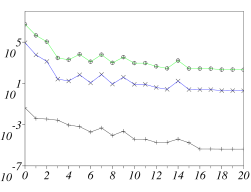
Refer to caption
Refer to caption
Refer to caption
Refer to caption
Figure 7: Algorithm 1 (left) and 2 (right) for Black–Scholes model with local “hyperbolic” volatility: Minimum ++, mean ×\times and maximum \circ of the (online) absolute variance (4.39) in a sample test ΛtestwidesubscriptΛtestwide\Lambda_{\rm testwide} of parameters with respect to the size I𝐼I of the reduced basis. Greedy selection with absolute variance (4.39) (top) and relative variance (4.40) (bottom).
Refer to caption
Refer to caption
Refer to caption
Refer to caption
Figure 8: Algorithm 1 (left) and 2 (right) for Black–Scholes model with local “hyperbolic” volatility: Minimum ++, mean ×\times and maximum \circ of the (online) relative variance (4.40) in a sample test ΛtestwidesubscriptΛtestwide\Lambda_{\rm testwide} of parameters with respect to the size I𝐼I of the reduced basis. Greedy selection with absolute variance (4.39) (top) and relative variance (4.40) (bottom).

4.2 Vector processes with constant diffusion and parametrized drift

4.2.1 Molecular simulation of dumbbells in polymeric fluids

In rheology of polymeric viscoelastic fluids, the long polymer molecules responsible for the viscoelastic behaviour can be modelled through kinetic theories of statistical physics as Rouse chains, that is as chains of Brownian beads connected by springs. We concentrate on the most simple of those models, namely “dumbbells” (two beads connected by one spring) diluted in a Newtonian fluid.

Kinetic models consist in adding to the usual velocity and pressure fields (𝒖,p)𝒖𝑝({\boldsymbol{u}},p) describing the (macroscopic) state of the Newtonian solvent, a field of dumbbells represented by their end-to-end vector 𝑿t(x)subscript𝑿𝑡𝑥{\boldsymbol{X}}_{t}(\uline{x}) at time t𝑡t and position x𝑥\uline{x} in the fluid. Vector stochastic processes (𝑿t(x))subscript𝑿𝑡𝑥({\boldsymbol{X}}_{t}(\uline{x})) encode the time evolution of the orientation and the stretch of the dumbbells (the idealized configuration of a polymer molecule) for each position x𝒟𝑥𝒟\uline{x}\in\mathcal{D} in a macroscopic domain 𝒟𝒟\mathcal{D} where the fluid flows. To compute the flow of a viscoelastic fluid with such multiscale dumbbell models [15], segregated algorithms are used that iteratively, on successive time steps with duration T𝑇T:

  • first evolve the velocity and pressure fields (𝒖,p)𝒖𝑝({\boldsymbol{u}},p)of the Newtonian solvent under a fixed extra (polymeric) stress tensor field 𝝉𝝉{\boldsymbol{\tau}}(typically following Navier-Stokes’equations), and

  • then evolve the (probability distribution of the) polymer configurations vector field (𝑿t(x))subscript𝑿𝑡𝑥({\boldsymbol{X}}_{t}(\uline{x})) surrounded by the newly computed fixed velocity field 𝒖𝒖{\boldsymbol{u}}.

The physics of kinetic models is based on a scale separation between the polymer molecules and the surrounding Newtonian fluid solvent. On the one side, the polymer configurations are directly influenced by the (local) velocity and pressure of the Newtonian solvent in which they are diluted. Reciprocally, on the other side, one needs to compute at every x𝒟𝑥𝒟\uline{x}\in\mathcal{D} the extra (polymeric) stress, given the Kramers formula:

𝝉(T,x)=𝔼(𝑿T(x)𝑭(𝑿T(x))),𝝉𝑇𝑥𝔼tensor-productsubscript𝑿𝑇𝑥𝑭subscript𝑿𝑇𝑥{\boldsymbol{\tau}}(T,\uline{x})=\mathbb{E}\left({\boldsymbol{X}}_{T}(\uline{x})\otimes{\boldsymbol{F}}({\boldsymbol{X}}_{T}(\uline{x}))\right)\,,

after one evolution step t[0,T]𝑡0𝑇t\in[0,T] over which the polymer configurations have evolved (remember that here [0,T]0𝑇[0,T] should be understood as a timestep). The vector valued process 𝑿t(x)subscript𝑿𝑡𝑥{\boldsymbol{X}}_{t}(\uline{x}) in dsuperscript𝑑\mathbb{R}^{d} (d=2𝑑2d=2 or 333) solves a Langevin equation at every physical point x𝒟𝑥𝒟\uline{x}\in\mathcal{D} (Eulerian description):

d𝑿t+𝒖x𝑿tdt=((x𝒖)𝑿t𝑭(𝑿t))dt+d𝑩t.𝑑subscript𝑿𝑡𝒖subscript𝑥subscript𝑿𝑡𝑑𝑡subscript𝑥𝒖subscript𝑿𝑡𝑭subscript𝑿𝑡𝑑𝑡𝑑subscript𝑩𝑡d{\boldsymbol{X}}_{t}+{\boldsymbol{u}}\cdot\nabla_{\uline{x}}{\boldsymbol{X}}_{t}dt=\left((\nabla_{\uline{x}}{\boldsymbol{u}})\,{\boldsymbol{X}}_{t}-{\boldsymbol{F}}({\boldsymbol{X}}_{t})\right)\,dt+d{\boldsymbol{B}}_{t}\,.

This Langevin equation describes the evolution of polymers at each x𝒟𝑥𝒟\uline{x}\in\mathcal{D}, under an advection 𝒖x𝑿t𝒖subscript𝑥subscript𝑿𝑡{\boldsymbol{u}}\cdot\nabla_{\uline{x}}{\boldsymbol{X}}_{t}, a hydrodynamic force (x𝒖)𝑿tsubscript𝑥𝒖subscript𝑿𝑡(\nabla_{\uline{x}}{\boldsymbol{u}}){\boldsymbol{X}}_{t}, Brownian collisions (𝑩t)subscript𝑩𝑡({\boldsymbol{B}}_{t}) with the solvent molecules, and an entropic force 𝑭(𝑿t)𝑭subscript𝑿𝑡{\boldsymbol{F}}({\boldsymbol{X}}_{t}) specific to the polymer molecules. Typically, this entropic force reads either 𝑭(𝑿)=𝑿𝑭𝑿𝑿{\boldsymbol{F}}({\boldsymbol{X}})={\boldsymbol{X}} (for Hookean dumbbells), or 𝑭(𝑿)=𝑿1|𝑿|2/b𝑭𝑿𝑿1superscript𝑿2𝑏{\boldsymbol{F}}({\boldsymbol{X}})=\frac{{\boldsymbol{X}}}{1-|{\boldsymbol{X}}|^{2}/b} (for Finitely-Extensible Nonlinear Elastic or FENE dumbells, to model the finite extensibility of polymers: |𝑿|<b𝑿𝑏|{\boldsymbol{X}}|<\sqrt{b}).

In the following, we do not consider the advection term 𝒖x𝑿t𝒖subscript𝑥subscript𝑿𝑡{\boldsymbol{u}}\cdot\nabla_{\uline{x}}{\boldsymbol{X}}_{t} (which can be handled through integration of the characteristics in a semi-Lagrangian framework, for instance), and we concentrate on solving the parametrized SDE:

d𝑿t=(λ𝑿t𝑭(𝑿t))dt+d𝑩t,𝑑subscript𝑿𝑡𝜆subscript𝑿𝑡𝑭subscript𝑿𝑡𝑑𝑡𝑑subscript𝑩𝑡d{\boldsymbol{X}}_{t}=\left(\uuline{\lambda}\,{\boldsymbol{X}}_{t}-{\boldsymbol{F}}({\boldsymbol{X}}_{t})\right)\,dt+d{\boldsymbol{B}}_{t}\,, (4.41)

on a time slab [0,T]0𝑇[0,T], with a fixed matrix λ(x)=x𝒖(x)𝜆𝑥subscript𝑥𝒖𝑥\uuline{\lambda}(\uline{x})=\nabla_{x}{\boldsymbol{u}}(\uline{x}). We also assume, as usual for viscoelastic fluids, that the velocity field is incompressible (that is tr(λ)=0tr𝜆0\mathrm{tr}(\uuline{\lambda})=0), hence the parameter λ𝜆\uuline{\lambda} is only (d21)superscript𝑑21(d^{2}-1)-dimensional.

This is a typical many-query context where the Langevin equation (4.41) has to be computed many times at each (discretized) position x𝒟𝑥𝒟\uline{x}\in\mathcal{D}, for each value of the d×d𝑑𝑑d\times d-dimensional parameter λ𝜆\uuline{\lambda} (since x𝒖(x)subscript𝑥𝒖𝑥\nabla_{\uline{x}}{\boldsymbol{u}}(\uline{x}) depends on the position x𝑥\uline{x}). Furthermore, the computation of the time-evolution of the flow defines a very demanding many-query context where the latter has to be done iteratively over numerous time steps of duration T𝑇T between which the tensor field λ(x)𝜆𝑥\uuline{\lambda}(\uline{x}) is evolved through a macroscopic equation for the velocity field 𝒖𝒖{\boldsymbol{u}}.

Remark 4.2 (Initial Condition of the SDE as additional parameter)

Let T0=0subscript𝑇00T_{0}=0 and Tn+1=(n+1)Tsubscript𝑇𝑛1𝑛1𝑇T_{n+1}=(n+1)T. Segregated numerical schemes for kinetic models of polymeric fluids as described above simulate (4.41) on successive time slabs [Tn,Tn+1]subscript𝑇𝑛subscript𝑇𝑛1[T_{n},T_{n+1}], for n𝑛n\in\mathbb{N}. More precisely, on each time slab [Tn,Tn+1]subscript𝑇𝑛subscript𝑇𝑛1[T_{n},T_{n+1}], one has to compute

𝝉(Tn+1)𝝉subscript𝑇𝑛1\displaystyle{\boldsymbol{\tau}}(T_{n+1}) =𝔼(𝑿Tn+1𝑭(𝑿Tn+1))absent𝔼tensor-productsubscript𝑿subscript𝑇𝑛1𝑭subscript𝑿subscript𝑇𝑛1\displaystyle=\mathbb{E}\left({\boldsymbol{X}}_{T_{n+1}}\otimes{\boldsymbol{F}}({\boldsymbol{X}}_{T_{n+1}})\right)
=𝔼(𝔼(𝑿Tn+1𝑭(𝑿Tn+1)|𝑿Tn))absent𝔼𝔼conditionaltensor-productsubscript𝑿subscript𝑇𝑛1𝑭subscript𝑿subscript𝑇𝑛1subscript𝑿subscript𝑇𝑛\displaystyle=\mathbb{E}\left(\mathbb{E}\left({\boldsymbol{X}}_{T_{n+1}}\otimes{\boldsymbol{F}}({\boldsymbol{X}}_{T_{n+1}})|{\boldsymbol{X}}_{T_{n}}\right)\right) (4.42)

at a fixed position x𝒟𝑥𝒟\uline{x}\in\mathcal{D}. In practice, (4.2) can be approximated through

𝝉(Tn+1)1Rr=1R1Mm=1M𝑿Tn+1r,m𝑭(𝑿Tn+1r,m),similar-to-or-equals𝝉subscript𝑇𝑛11𝑅superscriptsubscript𝑟1𝑅1𝑀superscriptsubscript𝑚1𝑀tensor-productsuperscriptsubscript𝑿subscript𝑇𝑛1𝑟𝑚𝑭superscriptsubscript𝑿subscript𝑇𝑛1𝑟𝑚{\boldsymbol{\tau}}(T_{n+1})\simeq\frac{1}{R}\sum_{r=1}^{R}\frac{1}{M}\sum_{m=1}^{M}{\boldsymbol{X}}_{T_{n+1}}^{r,m}\otimes{\boldsymbol{F}}({\boldsymbol{X}}_{T_{n+1}}^{r,m})\,, (4.43)

after simulating MR𝑀𝑅MR processes (𝐗tr,m)t[Tn,Tn+1]subscriptsuperscriptsubscript𝐗𝑡𝑟𝑚𝑡subscript𝑇𝑛subscript𝑇𝑛1({\boldsymbol{X}}_{t}^{r,m})_{t\in[T_{n},T_{n+1}]} driven by MR𝑀𝑅MR independent Brownian motions for a given set of R𝑅R different initial conditions, typically:

𝑿Tn+r,m=𝑿Tnr,1,r=1,,R,m=1,,M,formulae-sequencesuperscriptsubscript𝑿superscriptsubscript𝑇𝑛𝑟𝑚superscriptsubscript𝑿superscriptsubscript𝑇𝑛𝑟1formulae-sequence𝑟1𝑅𝑚1𝑀{\boldsymbol{X}}_{T_{n}^{+}}^{r,m}={\boldsymbol{X}}_{T_{n}^{-}}^{r,1}\,,\ r=1,\ldots,R\,,\ m=1,\ldots,M\,,

or any 𝐗Tnr,m0superscriptsubscript𝐗superscriptsubscript𝑇𝑛𝑟subscript𝑚0{\boldsymbol{X}}_{T_{n}^{-}}^{r,m_{0}} (with 1m0M1subscript𝑚0𝑀1\leq m_{0}\leq M) given by the computation at final time of the previous time slab [Tn1,Tn]subscript𝑇𝑛1subscript𝑇𝑛[T_{n-1},T_{n}]. In view of (4.43), for a fixed r𝑟r, the computation of 1Mm=1M𝐗Tn+1r,m𝐅(𝐗Tn+1r,m)1𝑀superscriptsubscript𝑚1𝑀tensor-productsuperscriptsubscript𝐗subscript𝑇𝑛1𝑟𝑚𝐅superscriptsubscript𝐗subscript𝑇𝑛1𝑟𝑚\frac{1}{M}\sum_{m=1}^{M}{\boldsymbol{X}}_{T_{n+1}}^{r,m}\otimes{\boldsymbol{F}}({\boldsymbol{X}}_{T_{n+1}}^{r,m}) using the algorithms presented above requires a modification of the methods to the case when the initial condition of the SDE assumes many values.

To adapt Algorithm 1 to the context of SDEs with many different initial conditions, one should consider reduced bases for control variates which depend on the joint-parameter (λ,x)𝜆𝑥({\lambda},x) where x𝑥x is the initial condition of the SDE. And variations on the joint-parameter (λ,x)𝜆𝑥({\lambda},x) can be simply recast into the framework of SDEs with fixed initial condition used for presentation of Algorithm 1 after the change of variable X^tλ,x=Xtλxsubscriptsuperscript^𝑋𝜆𝑥𝑡subscriptsuperscript𝑋𝜆𝑡𝑥\hat{X}^{\lambda,x}_{t}={X}^{\lambda}_{t}-x, that is using the family of SDEs with fixed initial condition X^λ,x0=0subscriptsuperscript^𝑋𝜆𝑥00{\hat{X}^{\lambda,x}}_{0}=0:

dX^tλ,x=b^λ,x(t,X^tλ,x)dt+σ^λ,x(t,X^tλ,x)dBt,𝑑subscriptsuperscript^𝑋𝜆𝑥𝑡superscript^𝑏𝜆𝑥𝑡subscriptsuperscript^𝑋𝜆𝑥𝑡𝑑𝑡superscript^𝜎𝜆𝑥𝑡subscriptsuperscript^𝑋𝜆𝑥𝑡𝑑subscript𝐵𝑡d{\hat{X}}^{\lambda,x}_{t}=\hat{b}^{\lambda,x}(t,\hat{X}^{\lambda,x}_{t})dt+\hat{\sigma}^{\lambda,x}(t,\hat{X}^{\lambda,x}_{t})d{B}_{t}\,, (4.44)

where b^λ,x(t,X)=bλ(t,X+x)superscript^𝑏𝜆𝑥𝑡𝑋superscript𝑏𝜆𝑡𝑋𝑥\hat{b}^{\lambda,x}(t,X)=b^{\lambda}(t,X+x), σ^λ,x(t,X)=σλ(t,X+x)superscript^𝜎𝜆𝑥𝑡𝑋superscript𝜎𝜆𝑡𝑋𝑥\hat{\sigma}^{\lambda,x}(t,X)=\sigma^{\lambda}(t,X+x), for all t𝑡t, X𝑋X and x𝑥x.Then, with g^λ,x(X)=gλ(X+x)superscript^𝑔𝜆𝑥𝑋superscript𝑔𝜆𝑋𝑥\hat{g}^{\lambda,x}(X)=g^{\lambda}(X+x) and f^λ,x(t,X)=fλ(t,X+x)superscript^𝑓𝜆𝑥𝑡𝑋superscript𝑓𝜆𝑡𝑋𝑥\hat{f}^{\lambda,x}(t,X)=f^{\lambda}(t,X+x), the output is the expectation of

Z^λ,x=g^λ(X^Tλ,x)0Tf^λ(s,X^sλ,x)𝑑s.superscript^𝑍𝜆𝑥superscript^𝑔𝜆superscriptsubscript^𝑋𝑇𝜆𝑥superscriptsubscript0𝑇superscript^𝑓𝜆𝑠superscriptsubscript^𝑋𝑠𝜆𝑥differential-d𝑠\hat{Z}^{\lambda,x}=\hat{g}^{\lambda}(\hat{X}_{T}^{\lambda,x})-\int_{0}^{T}\hat{f}^{\lambda}(s,\hat{X}_{s}^{\lambda,x})\,ds\,.

And the corresponding “ideal” control variate reads Y^λ,x=Z^λ,x𝔼(Z^λ,x).superscript^𝑌𝜆𝑥superscript^𝑍𝜆𝑥𝔼superscript^𝑍𝜆𝑥\hat{Y}^{\lambda,x}=\hat{Z}^{\lambda,x}-\mathbb{E}\left(\hat{Z}^{\lambda,x}\right)\,.

In Algorithm 2, note that uλsuperscript𝑢𝜆u^{\lambda} solution to (2.9) does not depend on the initial condition used for the SDE. So, once parameters λisubscript𝜆𝑖{\lambda_{i}} (i=1,,I𝑖1𝐼i=1,\ldots,I) have been selected offline, Algorithm 2 applies similarly for SDEs with one fixed, or many different, initial conditions. Though, the offline selection of parameters λisubscript𝜆𝑖{\lambda_{i}} using SDEs with many different initial conditions should consider a larger trial sample than for one fixed initial condition. Indeed, the selection criterium in the greedy algorithm does depend on the initial condition of the SDE. So, defining a trial sample of initial conditions ΛICsubscriptΛIC\Lambda_{\rm IC}, the following selection should be performed at step i𝑖i in Fig. 2:

Select λi+1argmaxλΛtrial\{λj,j=1,,i}maxxΛICVarMsmall(Zλ,xY~iλ,x),\textnormal{Select }\lambda_{i+1}\in\underset{\lambda\in\Lambda_{\rm trial}\backslash\{\lambda_{j},j=1,\ldots,i\}}{\operatornamewithlimits{arg\,max}}\underset{x\in\Lambda_{\rm IC}}{\max}{\rm Var_{M_{small}}}({Z}^{\lambda,x}-{\tilde{Y}^{\lambda,x}_{i}})\,,

where Zλ,xsuperscript𝑍𝜆𝑥{Z}^{\lambda,x} and Y~iλ,xsubscriptsuperscript~𝑌𝜆𝑥𝑖{\tilde{Y}^{\lambda,x}_{i}}, defined like Zλsuperscript𝑍𝜆Z^{\lambda} and Y~iλsubscriptsuperscript~𝑌𝜆𝑖\tilde{Y}^{\lambda}_{i}, depend on x𝑥x because the stochastic process (Xtλ)subscriptsuperscript𝑋𝜆𝑡(X^{\lambda}_{t}) depends on X0λ=xsubscriptsuperscript𝑋𝜆0𝑥X^{\lambda}_{0}=x.

It might be useful to build different reduced bases, one for each cell of a partition of the set of the initial condition. In summary, both algorithms can be extended to SDEs with variable initial condition, at the price of increasing the dimension of the parameter (see also Remark 4.1).

Remark 4.3 (Multi-dimensional output)

Clearly, the full output 𝛕𝛕{\boldsymbol{\tau}} in the problem described above is three-dimensional (it is a symmetric matrix). So our reduced-basis approach such as presented so far would need three different reduced bases, one for each scalar output. Though, one could alternatively consider the construction of only one reduced basis for the three outputs, which may be advantageous, see [4] for one example of such a construction.

Note that it is difficult to compute accurate approximations of the solution to the backward Kolmogorov equation (2.9) in the FENE case, because of the nonlinear explosive term. It is tractable in some situations, see [16, 6] for instance, though at the price of computational difficulties we did not want to deal with in this first work on our new variance reduction approach. On the contrary, the backward Kolmogorov equation (2.9) can be solved exactly in the case of Hookean dumbells. Hence we have approximated here uλsuperscript𝑢𝜆u^{\lambda} in Algorithm 2 by the numerical solution u~λsuperscript~𝑢𝜆\tilde{u}^{\lambda} to the backward Kolmogorov equation (2.9) for Hookean dumbells, whatever the type of dumbbells used for the molecular simulation (Hookean or FENE).

We would like to mention the recent work [14] where the classical reduced-basis method for parameterized PDEs has been used in the FENE case (solving the FENE Fokker-Planck by dedicated deterministic methods). Our approach is different since we consider a stochastic discretization.

4.2.2 Numerical results

The SDE (1.2) for FENE dumbbells (when d=2𝑑2d=2) is discretized with the Euler-Maruyama scheme using N=100𝑁100N=100 iterations with a constant time step of Δt=102Δ𝑡superscript102\Delta t=10^{-2} starting from a (deterministic) initial condition 𝑿0=(1,1)subscript𝑿011{\boldsymbol{X}}_{0}=(1,1), with reflecting boundary conditions at the boundary of the ball with radius b𝑏\sqrt{b}.

The number of realizations used for the Monte-Carlo evaluations, and the sizes of the (offline) trial sample ΛtrialsubscriptΛtrial\Lambda_{\rm trial} and (online) test sample ΛtestsubscriptΛtest\Lambda_{\rm test} for the three-dimensional matrix parameter λ𝜆\uuline{\lambda} with entries (λ11=λ22,λ12,λ21)subscript𝜆11subscript𝜆22subscript𝜆12subscript𝜆21(\lambda_{11}=-\lambda_{22},\lambda_{12},\lambda_{21}), are kept similar to the previous Section 4.1. Samples ΛtrialsubscriptΛtrial\Lambda_{\rm trial} and ΛtestsubscriptΛtest\Lambda_{\rm test} for the parameter λ𝜆\uuline{\lambda} are uniformly distributed in a cubic range Λ=[1,1]3Λsuperscript113\Lambda=[-1,1]^{3}. We will also make use of an enlarged (online) test sample ΛtestwidesubscriptΛtestwide\Lambda_{\rm testwide}, uniformly distributed in the range [2,2]3superscript223[-2,2]^{3}.

When b=9𝑏9b=9, the variance reduction online with Algorithm 1 is again very interesting, of about 444 orders of magnitude with I=20𝐼20I=20 basis functions, whatever the criterium used for the selection (we only show the absolute variance, in Fig. 11). But when b=4𝑏4b=4, the reflecting boundary conditions are more often active, and the maximum online variance reduction slightly degrades (see Fig. 11).
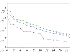
Refer to caption
Refer to caption
Figure 9: Algorithm 1 for FENE model with b=9𝑏9b=9: Minimum ++, mean ×\times and maximum \circ of the absolute variance (4.39) in samples of parameters (left: offline sample Λtrial{λi,i=1,,I}\Lambda_{\rm trial}\setminus\{\lambda_{i},i=1,\ldots,I\}; right: online sample ΛtestsubscriptΛtest\Lambda_{\rm test}) with respect to the size I𝐼I of the reduced basis.
Refer to caption
Refer to caption
Figure 10: Algorithm 1 for FENE model with b=4𝑏4b=4: Minimum ++, mean ×\times and maximum \circ of the absolute variance (4.39) in samples of parameters (left: offline sample Λtrial{λi,i=1,,I}\Lambda_{\rm trial}\setminus\{\lambda_{i},i=1,\ldots,I\}; right: online sample ΛtestsubscriptΛtest\Lambda_{\rm test}) with respect to the size I𝐼I of the reduced basis.
Refer to caption
Refer to caption
Figure 11: Algorithm 2 for FENE model with b=9𝑏9b=9: Minimum ++, mean ×\times and maximum \circ of the absolute variance (4.39) in samples of parameters (left: offline sample Λtrial{λi,i=1,,I}\Lambda_{\rm trial}\setminus\{\lambda_{i},i=1,\ldots,I\}; right: online sample ΛtestsubscriptΛtest\Lambda_{\rm test}) with respect to the size I𝐼I of the reduced basis.
Refer to caption
Refer to caption
Refer to caption
Refer to caption
Figure 12: Algorithm 1 (left) and 2 (right) for FENE model with b=16𝑏16b=16: Minimum ++, mean ×\times and maximum \circ of the relative variance (4.40) in online test for samples ΛtestsubscriptΛtest\Lambda_{\rm test} (top) and ΛtestwidesubscriptΛtestwide\Lambda_{\rm testwide} (bottom) of parameters, with respect to the size I𝐼I of the reduced basis.

We first tested our variance reduction with Algorithm 2 for Hookean dumbells and it appeared to work well; but such a model is considered too simple generally. Then using the solution to the Kolmogorov backward equation for Hookean dumbells as u~λsuperscript~𝑢𝜆\tilde{u}^{\lambda} in Algorithm 2 for FENE dumbbells still yields good variance reduction while the boundary is not touched (see Fig. 11) ; when b=4𝑏4b=4 and many reflections at the boundary occur, the variance is hardly reduced. Again Algorithm 2 seems to be slightly more robust than Algorithm 1 in terms of extrapolation, that is when the (online) test sample is “enlarged” (see Fig.12 with b=16𝑏16b=16 and a sample test (online) ΛtestwidesubscriptΛtestwide\Lambda_{\rm testwide}).

5 Conclusion and perspectives

We have demonstrated the feasibility of a reduced-basis approach to compute control variates for the expectation of functionals of a parameterized Itô stochastic process. We have also tested the efficiency of such an approach with two possible algorithms, in two simple test cases where either the drift or the diffusion of scalar (d=1𝑑1d=1), and vector (d=2𝑑2d=2), Itô processes are parametrized, using 222- or 333-dimensional parameters.

Algorithm 2 is less generic than Algorithm 1 ; it is basically restricted to low-dimensional stochastic processes (Xt)subscript𝑋𝑡(X_{t}) since:

  • one needs to solve (possibly high-dimensional) PDEs (offline), and

  • discrete approximations of the PDEs solutions on a grid have to be kept in memory (which is possibly a huge amount of data).

Yet, Algorithm 2 seems more robust to variations in the parameter.

From a theoretical viewpoint, it remains to better understand the convergence of reduced-basis approximations for parametrized control variates depending on the parametrization (and on the dimension of the parameter in particular), on the reduced-basis construction (following a greedy procedure)and on an adequate discretization choice (including the computation of approximate control variates and the choice of a trial sample ΛtrialsubscriptΛtrial\Lambda_{\rm trial}).

Acknowledgement. We acknowledge financial support from the France Israel Teamwork in Sciences. We thank Raz Kupferman, Claude Le Bris, Yvon Maday and Anthony T. Patera for fruitful discussions. We are grateful to the referees for constructive remarks.

Appendix A  Algorithm 2 in a higher-dimensional setting (d4𝑑4d\geq 4)

The solution uλ(t,y)superscript𝑢𝜆𝑡𝑦u^{\lambda}(t,y) to (2.9) can be computed at any (t,y)[0,T]×d𝑡𝑦0𝑇superscript𝑑(t,y)\in[0,T]\times\mathbb{R}^{d} by the martingale representation theorem [12]:

gλ(XTλ)tTfλ(s,Xsλ)𝑑s=uλ(t,Xtλ)+tTuλ(s,Xsλ)σλ(s,Xsλ)𝑑Bs,superscript𝑔𝜆superscriptsubscript𝑋𝑇𝜆superscriptsubscript𝑡𝑇superscript𝑓𝜆𝑠superscriptsubscript𝑋𝑠𝜆differential-d𝑠superscript𝑢𝜆𝑡subscriptsuperscript𝑋𝜆𝑡superscriptsubscript𝑡𝑇superscript𝑢𝜆𝑠superscriptsubscript𝑋𝑠𝜆superscript𝜎𝜆𝑠superscriptsubscript𝑋𝑠𝜆differential-dsubscript𝐵𝑠g^{\lambda}(X_{T}^{\lambda})-\int_{t}^{T}f^{\lambda}(s,X_{s}^{\lambda})ds=u^{\lambda}(t,X^{\lambda}_{t})+\int_{t}^{T}\nabla u^{\lambda}(s,X_{s}^{\lambda})\cdot\sigma^{\lambda}(s,X_{s}^{\lambda})dB_{s}, (6.45)

obtained by an Itô formula similar to (2.10). This gives the following Feynman-Kac formula for uλ(t,x)superscript𝑢𝜆𝑡𝑥u^{\lambda}(t,x), which can consequently be computed at any (t,y)[0,T]×d𝑡𝑦0𝑇superscript𝑑(t,y)\in[0,T]\times\mathbb{R}^{d} through Monte-Carlo evaluations:

uλ(t,y)=𝔼(gλ(XTλ,t,y)tTfλ(s,Xsλ,t,y)𝑑s),superscript𝑢𝜆𝑡𝑦𝔼superscript𝑔𝜆superscriptsubscript𝑋𝑇𝜆𝑡𝑦superscriptsubscript𝑡𝑇superscript𝑓𝜆𝑠superscriptsubscript𝑋𝑠𝜆𝑡𝑦differential-d𝑠u^{\lambda}(t,y)=\mathbb{E}\left(g^{\lambda}(X_{T}^{\lambda,t,y})-\int_{t}^{T}f^{\lambda}(s,X_{s}^{\lambda,t,y})ds\right), (6.46)

where (Xtλ,t0,y)t0tTsubscriptsuperscriptsubscript𝑋𝑡𝜆subscript𝑡0𝑦subscript𝑡0𝑡𝑇(X_{t}^{\lambda,t_{0},y})_{t_{0}\leq t\leq T} is the solution to (1.2) with initial condition Xt0λ,t0,y=ysuperscriptsubscript𝑋subscript𝑡0𝜆subscript𝑡0𝑦𝑦X_{t_{0}}^{\lambda,t_{0},y}=y. Differentiating (6.46) (provided fλsuperscript𝑓𝜆f^{\lambda} and gλsuperscript𝑔𝜆g^{\lambda} are differentiable), we even directly get a Feynman-Kac formula for uλ(t,y)superscript𝑢𝜆𝑡𝑦\nabla u^{\lambda}(t,y):

uλ(t,y)=𝔼(ΦTλ,t,ygλ(XTλ,t,y)tTΦsλ,t,yfλ(s,Xsλ,t,y)𝑑s)superscript𝑢𝜆𝑡𝑦𝔼superscriptsubscriptΦ𝑇𝜆𝑡𝑦superscript𝑔𝜆superscriptsubscript𝑋𝑇𝜆𝑡𝑦superscriptsubscript𝑡𝑇superscriptsubscriptΦ𝑠𝜆𝑡𝑦superscript𝑓𝜆𝑠superscriptsubscript𝑋𝑠𝜆𝑡𝑦differential-d𝑠\nabla u^{\lambda}(t,y)=\mathbb{E}\left(\Phi_{T}^{\lambda,t,y}\cdot\nabla g^{\lambda}(X_{T}^{\lambda,t,y})-\int_{t}^{T}\Phi_{s}^{\lambda,t,y}\cdot\nabla f^{\lambda}(s,X_{s}^{\lambda,t,y})ds\right) (6.47)

where the stochastic processes (Φsλ,t,y,s[t,T])superscriptsubscriptΦ𝑠𝜆𝑡𝑦𝑠𝑡𝑇\left(\Phi_{s}^{\lambda,t,y},s\in[t,T]\right) in d×dsuperscript𝑑𝑑\mathbb{R}^{d\times d} satisfy the first-order variation of the SDE (1.2) with respect to the initial condition, that is Φsλ,t,y=yXsλ,t,ysuperscriptsubscriptΦ𝑠𝜆𝑡𝑦subscript𝑦superscriptsubscript𝑋𝑠𝜆𝑡𝑦\Phi_{s}^{\lambda,t,y}=\nabla_{y}X_{s}^{\lambda,t,y} for any s[t,T]𝑠𝑡𝑇s\in[t,T]:

Φsλ,t,y=Idd+tsΦsλ,t,ybλ(s,Xsλ,t,y)𝑑s+tsΦsλ,t,yσλ(s,Xsλ,t,y)𝑑Bs,superscriptsubscriptΦ𝑠𝜆𝑡𝑦subscriptId𝑑superscriptsubscript𝑡𝑠superscriptsubscriptΦsuperscript𝑠𝜆𝑡𝑦superscript𝑏𝜆superscript𝑠superscriptsubscript𝑋superscript𝑠𝜆𝑡𝑦differential-dsuperscript𝑠superscriptsubscript𝑡𝑠superscriptsubscriptΦsuperscript𝑠𝜆𝑡𝑦superscript𝜎𝜆superscript𝑠superscriptsubscript𝑋superscript𝑠𝜆𝑡𝑦differential-dsubscript𝐵superscript𝑠\Phi_{s}^{\lambda,t,y}=\mbox{Id}_{d}+\int_{t}^{s}\Phi_{s^{\prime}}^{\lambda,t,y}\cdot\nabla b^{\lambda}(s^{\prime},X_{s^{\prime}}^{\lambda,t,y})ds^{\prime}+\int_{t}^{s}\Phi_{s^{\prime}}^{\lambda,t,y}\cdot\nabla\sigma^{\lambda}(s^{\prime},X_{s^{\prime}}^{\lambda,t,y})dB_{s^{\prime}}, (6.48)

where IddsubscriptId𝑑\mbox{Id}_{d} denotes the d×d𝑑𝑑{d\times d} identity matrix (see [21] for a more general and rigorous presentation of this Feynman-Kac formula in terms of the Malliavin gradient). The stochastic integral (2.11) can then be computed for each realization of (Bt)subscript𝐵𝑡(B_{t}), after discretizing (Φsλ,t,y,s[t,T])superscriptsubscriptΦ𝑠𝜆𝑡𝑦𝑠𝑡𝑇\left(\Phi_{s}^{\lambda,t,y},s\in[t,T]\right).

Discrete approximations of the Feynman-Kac formula (6.47) have already been used succesfully in the context of computing control variates for the reduction of variance, in [21] for instance. Note that this numerical strategy to compute uλsuperscript𝑢𝜆\nabla u^{\lambda}from a Feynman-Kac formula requires a lot of computations. Yet, most often, the computation time of the functions (t,y)uλ(t,y)𝑡𝑦superscript𝑢𝜆𝑡𝑦(t,y)\to\nabla u^{\lambda}(t,y) would not be a major issue in a reduced-basis approach, since this would be done offline (that is, in a pre-computation step, once for all) for only a few selected values of the parameter λ𝜆\lambda. What is nevertheless necessary for the reduced-basis approach to work is the possibility to store the big amount of data corresponding to a discretization of uλ(t,y)superscript𝑢𝜆𝑡𝑦\nabla u^{\lambda}(t,y) on a grid for the variable (t,y)[0,T]×d𝑡𝑦0𝑇superscript𝑑(t,y)\in[0,T]\times\mathbb{R}^{d}, (the parameter λ𝜆\lambda then assuming only a few values in ΛΛ\Lambda — of order 101010 in our numerical experiments —), and to have rapid access to those data in the online stage (where control variates are computed for any λΛ𝜆Λ\lambda\in\Lambda using those precomputed data).

Appendix B  Proof of Proposition 3.3

First note that, since 𝔼(Yλ)=0𝔼superscript𝑌𝜆0\mathbb{E}\left(Y^{\lambda}\right)=0, then 𝕍ar(Zλ)=𝕍ar(Yλ)𝕍arsuperscript𝑍𝜆𝕍arsuperscript𝑌𝜆{\rm\mathbb{V}ar}\left(Z^{\lambda}\right)={\rm\mathbb{V}ar}\left(Y^{\lambda}\right).

So, for all λΛ𝜆Λ\lambda\in\Lambda and for every linear combination of YλnNsuperscript𝑌subscriptsuperscript𝜆𝑁𝑛Y^{\lambda^{N}_{n}}, n=1,,N𝑛1𝑁n=1,\ldots,N :

YN=n=1Nan(λ)j=1Jgj(λnN)Yjsubscript𝑌𝑁superscriptsubscript𝑛1𝑁subscript𝑎𝑛𝜆superscriptsubscript𝑗1𝐽subscript𝑔𝑗superscriptsubscript𝜆𝑛𝑁subscript𝑌𝑗Y_{N}=\sum_{n=1}^{N}a_{n}(\lambda)\sum_{j=1}^{J}g_{j}(\lambda_{n}^{N})Y_{j}

(with any choice an(λ)subscript𝑎𝑛𝜆a_{n}(\lambda)\in\mathbb{R}, λnNΛsuperscriptsubscript𝜆𝑛𝑁Λ\lambda_{n}^{N}\in\Lambda, n=1,,N𝑛1𝑁n=1,\ldots,N), there holds (recall that the Yjsubscript𝑌𝑗Y_{j}, j=1,,J𝑗1𝐽j=1,\ldots,J, are uncorrelated) :

𝕍ar(ZλYN)𝕍arsuperscript𝑍𝜆subscript𝑌𝑁\displaystyle{\rm\mathbb{V}ar}\left(Z^{\lambda}-Y_{N}\right) =𝕍ar(YλYN)=Ω|j=1J(gj(λ)n=1Nan(λ)gj(λnN))Yj|2𝑑absent𝕍arsuperscript𝑌𝜆subscript𝑌𝑁subscriptΩsuperscriptsuperscriptsubscript𝑗1𝐽subscript𝑔𝑗𝜆superscriptsubscript𝑛1𝑁subscript𝑎𝑛𝜆subscript𝑔𝑗superscriptsubscript𝜆𝑛𝑁subscript𝑌𝑗2differential-d\displaystyle={\rm\mathbb{V}ar}\left(Y^{\lambda}-Y_{N}\right)=\int_{\Omega}\left|\sum_{j=1}^{J}\left(g_{j}(\lambda)-\sum_{n=1}^{N}a_{n}(\lambda)g_{j}(\lambda_{n}^{N})\right)\,Y_{j}\right|^{2}d\mathbb{P}
(j=1J|gj(λ)|2𝕍ar(Yj))sup1jJ|gj(λ)n=1Nan(λ)gj(λnN)|2|gj(λ)|2.absentsuperscriptsubscript𝑗1𝐽superscriptsubscript𝑔𝑗𝜆2𝕍arsubscript𝑌𝑗subscriptsupremum1𝑗𝐽superscriptsubscript𝑔𝑗𝜆superscriptsubscript𝑛1𝑁subscript𝑎𝑛𝜆subscript𝑔𝑗superscriptsubscript𝜆𝑛𝑁2superscriptsubscript𝑔𝑗𝜆2\displaystyle\leq\left(\sum_{j=1}^{J}|g_{j}(\lambda)|^{2}\>{\rm\mathbb{V}ar}\left(Y_{j}\right)\right)\sup_{1\leq j\leq J}\frac{\left|g_{j}(\lambda)-\sum_{n=1}^{N}a_{n}(\lambda)g_{j}(\lambda_{n}^{N})\right|^{2}}{|g_{j}(\lambda)|^{2}}\,. (7.49)

To get (3.30), we now explain how to choose the N𝑁N coefficients an(λ)subscript𝑎𝑛𝜆a_{n}(\lambda), 1nN1𝑛𝑁1\leq n\leq N, for each λΛ𝜆Λ\lambda\in\Lambda when λnNΛsuperscriptsubscript𝜆𝑛𝑁Λ\lambda_{n}^{N}\in\Lambda, n=1,,N𝑛1𝑁n=1,\ldots,N is given, and then how to choose those N𝑁N parameter values λnNΛsuperscriptsubscript𝜆𝑛𝑁Λ\lambda_{n}^{N}\in\Lambda, n=1,,N𝑛1𝑁n=1,\ldots,N.

Assume the N𝑁N parameter values λnNΛsuperscriptsubscript𝜆𝑛𝑁Λ\lambda_{n}^{N}\in\Lambda, n=1,,N𝑛1𝑁n=1,\ldots,N, are given, with λ0N=λminsuperscriptsubscript𝜆0𝑁subscript𝜆\lambda_{0}^{N}=\lambda_{\min}, λNN=λmaxsuperscriptsubscript𝜆𝑁𝑁subscript𝜆\lambda_{N}^{N}=\lambda_{\max} and λnNλn+1Nsuperscriptsubscript𝜆𝑛𝑁superscriptsubscript𝜆𝑛1𝑁\lambda_{n}^{N}\leq\lambda_{n+1}^{N}, n=0,,N1𝑛0𝑁1n=0,\ldots,N-1. Then, for a given M{2,,N}𝑀2𝑁M\in\{2,\ldots,N\} (to be determined later on) and for all λΛ𝜆Λ\lambda\in\Lambda, it is possible to choose 1M0(λ)N1subscript𝑀0𝜆𝑁1\leq M_{0}(\lambda)\leq N such that λM0(λ)NλλM0(λ)+M1Nsubscriptsuperscript𝜆𝑁subscript𝑀0𝜆𝜆subscriptsuperscript𝜆𝑁subscript𝑀0𝜆𝑀1\lambda^{N}_{M_{0}(\lambda)}\leq\lambda\leq\lambda^{N}_{M_{0}(\lambda)+M-1}. Only the M𝑀M coefficients corresponding to the M𝑀M contiguous parameter values above are taken non zero, such that λΛfor-all𝜆Λ\forall\lambda\in\Lambda :

am(λ)0M0(λ)mM0(λ)+M1,subscript𝑎𝑚𝜆0subscript𝑀0𝜆𝑚subscript𝑀0𝜆𝑀1{a}_{m}(\lambda)\neq 0\Leftrightarrow M_{0}(\lambda)\leq m\leq M_{0}(\lambda)+M-1\,,

and are more specifically chosen as am(λ)=Pmλ(τΛ(λ))subscript𝑎𝑚𝜆subscriptsuperscript𝑃𝜆𝑚subscript𝜏Λ𝜆{a}_{m}(\lambda)=P^{\lambda}_{m}(\tau_{\Lambda}(\lambda)) where Pmλsubscriptsuperscript𝑃𝜆𝑚P^{\lambda}_{m} are polynomials of degree M1𝑀1M-1, such that, for all M0(λ)m,kM0(λ)+M1formulae-sequencesubscript𝑀0𝜆𝑚𝑘subscript𝑀0𝜆𝑀1M_{0}(\lambda)\leq m,k\leq M_{0}(\lambda)+M-1, Pmλ(τΛ(λk))=δmksubscriptsuperscript𝑃𝜆𝑚subscript𝜏Λsubscript𝜆𝑘subscript𝛿𝑚𝑘P^{\lambda}_{m}(\tau_{\Lambda}(\lambda_{k}))=\delta_{mk}. The polynomial function Pmλsubscriptsuperscript𝑃𝜆𝑚P^{\lambda}_{m} is the Lagrange interpolant defined on [τΛ(λM0(λ)),τΛ(λM0(λ)+M1)]subscript𝜏Λsubscript𝜆subscript𝑀0𝜆subscript𝜏Λsubscript𝜆subscript𝑀0𝜆𝑀1[\tau_{\Lambda}(\lambda_{M_{0}(\lambda)}),\tau_{\Lambda}(\lambda_{M_{0}(\lambda)+M-1})], taking value 111 at τΛ(λm)subscript𝜏Λsubscript𝜆𝑚\tau_{\Lambda}(\lambda_{m}) and 00 at τΛ(λk)subscript𝜏Λsubscript𝜆𝑘\tau_{\Lambda}(\lambda_{k}), km𝑘𝑚k\neq m. We will also need a function d(λ)=|τ(λM0(λ))τ(λM0(λ)+M1)|𝑑𝜆𝜏subscript𝜆subscript𝑀0𝜆𝜏subscript𝜆subscript𝑀0𝜆𝑀1d(\lambda)=|\tau(\lambda_{M_{0}(\lambda)})-\tau(\lambda_{M_{0}(\lambda)+M-1})|. Using a Taylor-Lagrange formula for gjτ1subscript𝑔𝑗superscript𝜏1g_{j}\circ\tau^{-1}, we have (for some 0η10𝜂10\leq\eta\leq 1) :

gj(λ)n=1Nanλ(λ)gj(λn)=d(λ)MM!(gjτ1)(M)(ητ(λM0(λ)N)+(1η)τ(λM0(λ)+M1N)).subscript𝑔𝑗𝜆superscriptsubscript𝑛1𝑁subscriptsuperscript𝑎𝜆𝑛𝜆subscript𝑔𝑗subscript𝜆𝑛𝑑superscript𝜆𝑀𝑀superscriptsubscript𝑔𝑗superscript𝜏1𝑀𝜂𝜏superscriptsubscript𝜆subscript𝑀0𝜆𝑁1𝜂𝜏superscriptsubscript𝜆subscript𝑀0𝜆𝑀1𝑁g_{j}(\lambda)-\sum_{n=1}^{N}a^{\lambda}_{n}(\lambda)g_{j}(\lambda_{n})=\frac{d(\lambda)^{M}}{M!}(g_{j}\circ\tau^{-1})^{(M)}\left(\eta\tau(\lambda_{M_{0}(\lambda)}^{N})+(1-\eta)\tau(\lambda_{M_{0}(\lambda)+M-1}^{N})\right)\,.

Then, using (3.29) and the fact that 𝕍ar(Zλ)=j=1J|gj(λ)|2𝕍ar(Yj)𝕍arsuperscript𝑍𝜆superscriptsubscript𝑗1𝐽superscriptsubscript𝑔𝑗𝜆2𝕍arsubscript𝑌𝑗{\rm\mathbb{V}ar}\left(Z^{\lambda}\right)=\sum_{j=1}^{J}|g_{j}(\lambda)|^{2}\>{\rm\mathbb{V}ar}\left(Y_{j}\right), there exists a constant C>0𝐶0C>0 (independent of ΛΛ\Lambda and J𝐽J) such that:

𝕍ar(ZλYN)𝕍ar(Zλ)(Cd(λ))2M,λΛ.formulae-sequence𝕍arsuperscript𝑍𝜆subscript𝑌𝑁𝕍arsuperscript𝑍𝜆superscript𝐶𝑑𝜆2𝑀for-all𝜆Λ{\rm\mathbb{V}ar}\left(Z^{\lambda}-Y_{N}\right)\leq{\rm\mathbb{V}ar}\left(Z^{\lambda}\right)\,\left(C\>d(\lambda)\right)^{2M}\,,\ \forall\lambda\in\Lambda\,. (7.50)

Finally, to get the result, we now choose a τΛsubscript𝜏Λ\tau_{\Lambda}-equidistributed parameter sample :

τΛ(λnN)=τΛ(λmin)+n1N1(τΛ(λmax)τΛ(λmin)),n=1,,N.formulae-sequencesubscript𝜏Λsuperscriptsubscript𝜆𝑛𝑁subscript𝜏Λsubscript𝜆𝑛1𝑁1subscript𝜏Λsubscript𝜆subscript𝜏Λsubscript𝜆𝑛1𝑁\tau_{\Lambda}(\lambda_{n}^{N})=\tau_{\Lambda}(\lambda_{\min})+\frac{n-1}{N-1}\left(\tau_{\Lambda}(\lambda_{\max})-\tau_{\Lambda}(\lambda_{\min})\right)\,,\ n=1,\ldots,N\,.

Then, d(λ)=M1N1(τΛ(λmax)τΛ(λmin))𝑑𝜆𝑀1𝑁1subscript𝜏Λsubscript𝜆subscript𝜏Λsubscript𝜆d(\lambda)=\frac{M-1}{N-1}\left(\tau_{\Lambda}(\lambda_{\max})-\tau_{\Lambda}(\lambda_{\min})\right) does not depend on λ𝜆\lambda. Minimizing (Cd)dsuperscript𝐶𝑑𝑑(C\,d)^{d} as a function of d(0,1C)𝑑01𝐶d\in(0,\frac{1}{C}), we choose d(λ)=1eC𝑑𝜆1𝑒𝐶d(\lambda)=\frac{1}{e\>C}, and the choice M=1+1eCN1τΛ(λmax)τΛ(λmin)𝑀11𝑒𝐶𝑁1subscript𝜏Λsubscript𝜆subscript𝜏Λsubscript𝜆M=1+\lfloor\frac{1}{e\>C}\frac{N-1}{\tau_{\Lambda}(\lambda_{\max})-\tau_{\Lambda}(\lambda_{\min})}\rfloor (where x𝑥\lfloor x\rfloor denotes the integer part of a real number x𝑥x\in\mathbb{R}) finishes the proof provided NN01+Ce(τΛ(λmax)τΛ(λmin))𝑁subscript𝑁01𝐶𝑒subscript𝜏Λsubscript𝜆subscript𝜏Λsubscript𝜆N\geq N_{0}\equiv 1+\lfloor C\>e\>\left(\tau_{\Lambda}(\lambda_{\max})-\tau_{\Lambda}(\lambda_{\min})\right)\rfloor. \ \square

References

  • [1] Y. Achdou and O. Pironneau, Computational Methods for Option Pricing (Frontiers in Applied Mathematics 30). Society for Industrial and Applied Mathematics, 2005.
  • [2] B. Arouna, Robbins-Monroe algorithms and variance reduction in finance. The Journal of Computational Finance 7(2):35–62, 2004.
  • [3] J. Bonvin and M. Picasso, Variance reduction methods for CONNFFESSIT-like simulations. J. Non-Newtonian Fluid Mech 84:191–215, 1999.
  • [4] S. Boyaval, Reduced-basis approach for homogenization beyond the periodic setting. SIAM Multiscale Modeling and Simulation 7(1):466–494, 2008.
  • [5] S. Boyaval, C. Le Bris, Y. Maday, N.C. Nguyen, and A.T. Patera, A Reduced Basis Approach for Variational Problems with Stochastic Parameters: Application to Heat Conduction with Variable Robin Coefficient. Accepted for publication in CMAME. INRIA preprint RR-6617, available at http://hal.inria.fr/inria-00311463.
  • [6] C. Chauvière and A. Lozinski, Simulation of dilute polymer solutions using a Fokker-Planck equation. Computers and Fluids 33:687–696, 2004.
  • [7] A. Friedman, Stochastic differential equations and applications, Vol. 1. Academic Press (New York ; London ; Toronto), 1975.
  • [8] G. Golub and C. van Loan, Matrix computations, third edition. The Johns Hopkins University Press, London, 1996.
  • [9] G. Grimmett and D. Stirzaker, Probability and Random Processes. 2nd ed. Oxford, 1992.
  • [10] J. Hammersley and D. Handscomb, eds., Monte Carlo Methods. Chapman and Hall Ltd, London, 1964.
  • [11] B. Jourdain, Adaptive variance reduction techniques in finance, to appear in Radon Series Comp. Appl. Math 8. De Gruyter, 2009.
  • [12] I. Karatzas and S.E. Shreve, Brownian Motion and Stochastic Calculus. SpringerVerlag, 1991.
  • [13] P. Kloeden and E. Platen, Numerical Solution of Stochastic Differential Equations. Springer, 2000.
  • [14] DJ Knezevic and AT Patera, A Certified Reduced Basis Method for the Fokker-Planck Equation of Dilute Polymeric Fluids: FENE Dumbbells in Extensional Flow. SIAM Journal of Scientific Computing (submitted).
  • [15] C. Le Bris and T. Lelièvre, Multiscale modelling of complex fluids: A mathematical initiation, in Multiscale Modeling and Simulation in Science Series, B. Engquist, P. Lötstedt, O. Runborg, eds., Lecture Notes in Computational Science and Engineering 66, Springer, 49–138, 2009.
  • [16] A. Lozinski and C. Chauvière, A fast solver for Fokker-Planck equations applied to viscoelastic flows calculations: 2D FENE model, J. Comput. Phys., 189:607–625, 2003.
  • [17] L. Machiels, Y. Maday, and A.T. Patera. Output bounds for reduced-order approximations of elliptic partial differential equations. Comput. Methods Appl. Mech. Engrg., 190(26-27):3413–3426, 2001.
  • [18] Y. Maday and A.T. Patera and G. Turinici, A Priori Convergence Theory for Reduced-Basis Approximations of Single-Parameter Elliptic Partial Differential Equations. Journal of Scientific Computing, 17(1-4):437–446, 2002.
  • [19] M. Melchior and H.C. Öttinger, Variance reduced simulations of stochastic differential equations. J. Chem. Phys. 103:9506–9509, 1995.
  • [20] G.N. Milstein and M.V. Tretyakov, Practical variance reduction via regression for simulating diffusions. Technical Report MA-06-19, School of Mathematics and Computer Science, University of Leicester, 2006.
  • [21] N.J. Newton, Variance reduction for simulated diffusions, SIAM J. Appl. Math.. 54(6):1780–1805, 1994.
  • [22] H.C. Öttinger, B.H.A.A. van den Brule and M. Hulsen, Brownian configuration fields and variance reduced CONNFFESSIT, J. Non-Newtonian Fluid Mech. 70:25 – 261, 1997.
  • [23] A.T. Patera and G. Rozza, Reduced Basis Approximation and A Posteriori Error Estimation for Parametrized Partial Differential Equations, Version 1.0, Copyright MIT 2006 - 2007, to appear in (tentative rubric) MIT Pappalardo Graduate Monographs in Mechanical Engineering.
  • [24] O. Pironneau, Calibration of options on a reduced basis, Journal of Computational and Applied Mathematics. In Press, Corrected Proof, 2008. DOI: 10.1016/j.cam.2008.10.070.
  • [25] S. Sen, Reduced-Basis Approximation and A Posteriori Error Estimation for Many-Parameter Heat Conduction Problems. Numerical Heat Transfer, Part B: Fundamentals 54(5):69–389, 2008.