Huffman Coding as a Non-linear Dynamical System

Abstract

In this paper, source coding or data compression is viewed as a measurement problem. Given a measurement device with fewer states than the observable of a stochastic source, how can one capture the essential information? We propose modeling stochastic sources as piecewise linear discrete chaotic dynamical systems known as Generalized Luröth Series (GLS) which dates back to Georg Cantor’s work in 1869. The Lyapunov exponent of GLS is equal to the Shannon’s entropy of the source (up to a constant of proportionality). By successively approximating the source with GLS having fewer states (with the closest Lyapunov exponent), we derive a binary coding algorithm which exhibits minimum redundancy (the least average codeword length with integer codeword lengths). This turns out to be a re-discovery of Huffman coding, the popular lossless compression algorithm used in the JPEG international standard for still image compression.

I Source Coding seen as a Measurement Problem

A practical problem an experimental physicist would face is the following – a process (eg. a particle moving in space) has an observed variable (say position of the particle) which potentially takes $N$ distinct values, but the measuring device is capable of recording only $M$ values and $M<N$. In such a scenario (Figure 1), how can we make use of these $M$ states of the measuring device to capture the essential information of the source? It may be the case that $N$ takes values from an infinite set, but the measuring device is capable of recording only a finite number of states. However, it shall be assumed that $N$ is finite but allowed for the possibility that $N\gg M$ (for e.g., it is possible that $N=10^{6}$ and $M=2$).

Our aim is to capture the essential information of the source (the process is treated as a source and the observations as messages from the source) in a lossless fashion. This problem actually goes all the way back to Shannon Shannon1948 who gave a mathematical definition for the information content of a source. He defined it as ‘Entropy’, a term borrowed from statistical thermodynamics. Furthermore, his now famous noiseless source coding theorem states that it is possible to encode the information of a memoryless source (assuming that the observables are independent and identically distributed (i.i.d)) using (at least) $H(X)$ bits per symbol, where $H(X)$ stands for the Shannon’s entropy of the source $X$. Stated in other words, the average codeword length $\sum_{i}l_{i}p_{i}\leq H(X)$ where $l_{i}$ is the length of the $i$-th codeword and $p_{i}$ the corresponding probability of occurrence of the $i$-th alphabet of the source.

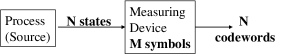
Figure 1: Source coding as a measurement problem. Typically, $M\ll N$. If $M=2$, we are seeking binary codes.

Shannon’s entropy $H(X)$ defines the ultimate limit for lossless data compression. Data compression is a very important and exciting research topic in Information theory since it not only provides a practical way to store bulky data, but it can also be used effectively to measure entropy, estimate complexity of sequences and provide a way to generate pseudo-random numbers MacKay (which are necessary for Monte-Carlo simulations and Cryptographic protocols).

Several researchers have investigated the relationship between chaotic dynamical systems and data compression (more generally between chaos and information theory). Jiménez-Montaño, Ebeling, and others nsrps1 have proposed coding schemes by a symbolic substitution method. This was shown to be an optimal data compression algorithm by Grassberger Grassberger and also to accurately estimate Shannon’s entropy Grassberger and Lyapunov exponents of dynamical systems nsrps2 . Arithmetic coding, a popular data compression algorithm used in JPEG2000 was recently shown to be a specific mode of a piecewise linear chaotic dynamical system NithinAC . In another work NithinKraft , we have used symbolic dynamics on chaotic dynamical systems to prove the famous Kraft-McMillan inequality and its converse for prefix-free codes, a fundamental inequality in source coding, which also has a Quantum analogue.

In this paper, we take a nonlinear dynamical systems approach to the aforementioned measurement problem. We are interested in modeling the source by a nonlinear dynamical system. By a suitable model, we hope to capture the information content of the source. This paper is organized as follows. In Section II, stochastic sources are modeled using piecewise linear chaotic dynamical systems which exhibits some important and interesting properties. In Section III, we propose a new algorithm for source coding and prove that it achieves the least average codeword length and turns out to be a re-discovery of Huffman coding Huffman1952 – the popular lossless compression algorithm used in the JPEG international standard JPEG for still image compression. We make some observations about our approach in Section IV and conclude in Section V.

II Source Modeling using Piecewise Linear Chaotic Dynamical Systems

We shall consider stationary sources. These are defined as sources whose statistics remain constant with respect to time Papoulis2002 . These include independent and identically distributed (i.i.d) sources and Ergodic (Markov) sources. These sources are very important in modeling various physical/chemical/biological phenomena and in engineering applications Kohda2002 .

On the other hand, non-stationary sources are those whose statistics change with time. We shall not deal with them here. However, most coding methods are applicable to these sources with some suitable modifications.

II.1 Embedding an i.i.d Source using Generalized Luröth Series

Consider an i.i.d source $X$ (treated as a random variable) which takes values from a set of $N$ values $\mathcal{A}=\{a_{1},a_{2},\ldots,a_{N}\}$ with probabilities $\{p_{1},p_{2},\ldots,p_{N}\}$ respectively with the condition $\sum_{1}^{N}p_{i}=1$.

An i.i.d source can be simply modeled as a (memoryless) Markov source (or Markov process Papoulis2002 ) with the transition probability from state $i$ to $j$ as being independent of state $i$ (and all previous states) . We can then embed the Markov source into a dynamical system as follows: to each Markov state (i.e. to each symbol in the alphabet), associate an interval on the real line segment $[0,1)$ such that its length is equal to the probability. Any two such intervals have pairwise disjoint interiors and the union of all the intervals cover $[0,1)$. Such a collection of intervals is known as a partition. We define a deterministic map $T$ on the partitions such that they form a Markov partition (they satisfy the property that the image of each interval under $T$ covers an integer number of partitions Afraimovich2003 ).

The simplest way to define the map $T$ such that the intervals form a Markov partition is to make it linear and surjective. This is depicted in Figure 2(a). Such a map is known as Generalized Luröth Series (GLS). There are other ways to define the map $T$ (for eg., see Kohda2002 ) but for our purposes GLS will suffice. Luröth’s paper in 1883 (see reference in Dajani et. al. Dajani2002 ) deals with number theoretical properties of Luröth series (a specific case of GLS). However, Georg Cantor had discovered GLS earlier in 1869 Waterman1975 ; Cantor1869 .

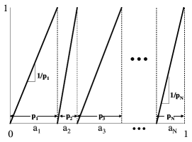
(a) Generalized Luröth Series (GLS) $T:[0,1)\mapsto[0,1)$
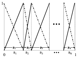
(b) $2^{N}$ modes of GLS.

Figure 2: Embedding an i.i.d source into a Generalized Luröth Series (GLS).

II.2 Some Important Properties of GLS

A list of important properties of GLS is given below:

1. GLS preserves the Lebesgue (probability) measure.

2. Every (infinite) sequence of symbols from the alphabet corresponds to an unique initial condition.

3. The symbolic sequence of every initial condition is i.i.d.

4. GLS is Chaotic (positive Lyapunov exponent, positive Topological entropy).

5. GLS has maximum topological entropy ($=ln(N)$) for a specified number of alphabets ($N$). Thus, all possible arrangements of the alphabets can occur as symbolic sequences.

6. GLS is isomorphic to the Shift map and hence Ergodic (Bernoulli).

7. Modes of GLS: As it can be seen from Figure 2(b), the slope of the line that maps each interval to $[0,1)$ can be chosen to be either positive or negative. These choices result in a total of $2^{N}$ modes of GLS (up to a permutation of the intervals along with their associated alphabets for each mode, these are $N!$ in number).

It is property 2 and 3 that allow a faithful “embedding” of a stochastic i.i.d source. For a proof of these properties, please refer Dajani et. al. Dajani2002 . Some well known GLS are the standard Binary map and the standard Tent map shown in Figure 3.

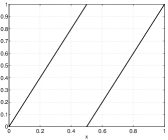
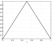
(a)                                   (b)

Figure 3: Some well known GLS: (a) Standard Binary map ($x\mapsto 2x$, $0\leq x<0.5$; $x\mapsto 2x-1$, $0.5\leq x<1$). (b) Standard Tent map ($x\mapsto 2x$, $0\leq x<0.5$; $x\mapsto 2-2x$, $0.5\leq x<1$).

II.3 Lyapunov Exponent of GLS = Shannon’s Entropy

It is easy to verify that GLS preserves the Lebesgue measure. A probability density $\Pi(x)$ on [0,1) is invariant under the given transformation $T$, if for each interval $[c,d]\subset[0,1)$, we have:

$$\int_{c}^{d}\Pi(x)dx=\int_{\mathcal{S}}\Pi(x)dx.$$ (1)

where $\mathcal{S}=T^{-1}([c,d])=\{x|c\leq T(x)\leq d\}$.

For the GLS, the above condition has constant probability density on $[0,1)$ as the only solution. It then follows from Birkhoff’s ergodic theorem Dajani2002 that the asymptotic probability distribution of the points of almost every trajectory is uniform. We can hence calculate Lyapunov exponent as follows:

$$\lambda=\int_{0}^{1}log_{2}(|T^{\prime}(x)|)\Pi(x)dx.~{}~{}~{}\textrm{(almost everywhere)}$$ (2)

Here, we measure $\lambda$ in bits/iteration.

$\Pi(x)$ is uniform with value 1 on [0,1) and $T^{\prime}(x)=constant$ since $T(x)$ is linear in each of the intervals, the above expression simplifies to:

$$\lambda=-\sum_{i=1,p_{i}\neq 0}^{i=N}p_{i}log_{2}(p_{i}).~{}~{}~{}\textrm{(almost everywhere)}$$ (3)

This turns out to be equal to Shannon’s entropy of the i.i.d source $X$. Thus Lyapunov exponent of the GLS that faithfully embeds the stochastic i.i.d source $X$ is equal to the Shannon’s entropy of the source. Lyapunov exponent can be understood as the amount of information in bits revealed by the symbolic sequence (measurement) of the dynamical system in every iteration . It can be seen that the Lyapunov exponent for all the modes of the GLS are the same. The Lyapunov exponent for binary i.i.d sources is plotted in Figure 4 as a function of $p$ (the probability of symbol ‘0’).

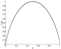
Figure 4: Lyapunov Exponent: $\lambda(p)=-p\log_{2}(p)-(1-p)\log_{2}(1-p)$ in units of bits/iteration plotted against $p$ for binary i.i.d sources. The maximum occurs at $p=\frac{1}{2}$. Note that $\lambda(p)=\lambda(1-p)$.

III Successive Source Approximation using GLS

In this section, we address the measurement problem proposed in Section I. Throughout our analysis, $N>2$ (finite) and $M=2$ is assumed. We are seeking minimum-redundancy binary symbol codes. “Minimum-redundancy” is defined as follows Huffman1952 :

Definition 1 (Minimum Redundancy)

A binary symbol code $\mathcal{C}=\{c_{1},c_{2},\ldots,c_{N}\}$ with lengths $L=\{l_{1},l_{2},\ldots,l_{N}\}$ for the i.i.d source $X$ with alphabet $\mathcal{A}=\{a_{1},a_{2},\ldots,a_{N}\}$ with respective probabilities $\{p_{1},p_{2},\ldots,p_{N}\}$ is said to have minimum-redundancy if $L_{\mathcal{C}}(X)=\sum_{i=1}^{N}l_{i}p_{i}$ is minimum.

For $N=2$, the minimum-redundancy binary symbol code for the alphabet $\mathcal{A}=\{a_{1},a_{2}\}$ is $\mathcal{C}=\{0,1\}$ ($a_{1}\mapsto 0$, $a_{2}\mapsto 1$). The goal of source coding is to minimize $L_{\mathcal{C}}(X)$, the average code-word length of $\mathcal{C}$, since this is important in any communication system. As we mentioned before, it is always true that $L_{\mathcal{C}}(X)\geq H(X)$ Shannon1948 .

III.1 Successive Source Approximation Algorithm using GLS

Our approach is to approximate the original i.i.d source (GLS with $N$ partitions) with the best GLS with a reduced number of partitions (reduced by 1). For the sake of notational convenience, we shall term the original GLS as order $N$ (for original source $X_{N}$) and the reduced GLS would be of order $N-1$ (for approximating source $X_{N-1}$). This new source $X_{N-1}$ is now approximated further with the best possible source of order $N-2$ ($X_{N-2}$). This procedure of successive approximation of sources is repeated until we end up with a GLS of order $M=2$ ($X_{2}$). It has only two partitions for which we know the minimum-redundancy symbol code is $\mathcal{C}=\{0,1\}$.

At any given stage $q$ of approximation, the easiest way to construct a source of order $q-1$ is to merge two of the existing $q$ partitions. What should be the rationale for determining which is the best $q-1$ order approximating source $X_{q-1}$ for the source $X_{q}$?

Definition 2 (Best Approximating Source)

Among all possible $q-1$ order approximating sources, the best approximation is the one which minimizes the following quantity:

$$\Delta=\lambda(X_{q})-\lambda(X_{q-1}).$$ (4)

where $\lambda(\cdot)$ is the Lyapunov exponent of the argument. The reason behind this choice is intuitive. We have already established that the Lyapunov exponent is equal to the Shannon’s entropy for the GLS and that it represents the amount of information (in bits) revealed by the symbolic sequence of the source at every iteration. Thus, the best approximating source should be as close as possible to the original source in terms of Lyapunov exponent.

There are three steps to our algorithm for finding minimum redundancy binary symbol code as given below here:

Algorithm 1 Successive Source Approximation using GLS

1. Embed the i.i.d source $X$ in to a GLS with $N$ partitions as described in II.1. Initialize $K=N$. The source is denoted by $X_{K}$ to indicate order $K$.

2. Approximate source $X_{K}$ with a GLS with $K-1$ partitions by merging the smallest two partitions to obtain the source $X_{K-1}$ of order $K-1$. $K\leftarrow K-1$.

3. Repeat step 2 until order of the GLS is 2 ($K=2$), then, stop.

We shall prove that the approximating source which merges the two smallest partitions is the best approximating source. It shall be subsequently proved that this algorithm leads to minimum-redundancy, i.e., it minimizes $L_{\mathcal{C}}(X)$. Assigning codewords to the alphabets will also be shown.

Theorem 1: (Best Successive Source Approximation) For a source $X_{M}$ which takes values from $\{A_{1},A_{2},\ldots A_{M-1},A_{M}\}$ with probabilities $\{p_{1},p_{2},\ldots p_{M-1},p_{M}\}$ respectively and with $1\geq p_{1}\geq p_{2}\geq\ldots\geq p_{M-1}\geq p_{M}\geq 0$ ($\sum_{i=1}^{i=M}p_{i}=1$), the source $X_{M-1}$ which is the best $M$-1 order approximation to $X_{M}$ has probabilities $\{p_{1},p_{2},\ldots p_{M-2},p_{M-1}+p_{M}\}$.

Proof:
By induction on $M$. For $M=1$ and $M=2$, there is nothing to prove. We will first show that the statement is true for $M=3$.

• $M=3$. $X_{3}$ takes values from $\{a_{1},a_{2},a_{3}\}$ with probabilities $\{p_{1},p_{2},p_{3}\}$ respectively and $1\geq p_{1}\geq p_{2}\geq p_{3}\geq 0$ with $p_{1}+p_{2}+p_{3}=1$.
  

  We need to show that $X_{2}$ which takes values from $\{a_{1},Z\}$ with probabilities $\{p_{1},p_{2}+p_{3}\}$ is the best $2$-order approximation to $X_{3}$. Here $Z$ is a symbol that represents the merged partition.
  

  This means, that we should show that this is better than any other $2$-order approximation. There are two other $2$-order approximations, namely, $Y_{2}$ which takes values from $\{a_{3},Z\}$ with probabilities $\{p_{3},p_{2}+p_{1}\}$ and $W_{2}$ which takes values from $\{a_{2},Z\}$ with probabilities $\{p_{2},p_{1}+p_{3}\}$.
  

  This implies that we need to show $\lambda(X_{3})-\lambda(X_{2})\leq\lambda(X_{3})-\lambda(Y_{2})$ and $\lambda(X_{3})-\lambda(X_{2})\leq\lambda(X_{3})-\lambda(W_{2})$.

• We shall prove $\lambda(X_{3})-\lambda(X_{2})\leq\lambda(X_{3})-\lambda(Y_{2})$.

  This means that we need to prove $\lambda(X_{2})\geq\lambda(Y_{2})$. This means we need to show $-p_{1}log_{2}(p_{1})-(p_{2}+p_{3})log_{2}(p_{2}+p_{3})\geq-p_{3}log_{2}(p_{3})-(p_{1}+p_{2})log_{2}(p_{1}+p_{2})$. We need to show the following:

  $$-p_{1}log_{2}(p_{1})-(1-p_{1})log_{2}(1-p_{1}) \geq -p_{3}log_{2}(p_{3})$$

  $$-(1-p_{3})log_{2}(1-p_{3})$$

  $$\Rightarrow\lambda_{2}(p_{1}) \geq \lambda_{2}(p_{3}).$$

  There are two cases. If $p_{1}\leq 0.5$, then since $p_{3}\leq p_{1}$, $\lambda_{2}(p_{1})\geq\lambda_{2}(p_{3})$. If $p_{1}>0.5$, then since $p_{2}+p_{3}=1-p_{1}$, we have $p_{3}\leq 1-p_{1}$. This again implies $\lambda_{2}(p_{1})\geq\lambda_{2}(p_{3})$. Thus, we have proved that $X_{2}$ is better than $Y_{2}$.

• We can follow the same argument to prove that $\lambda(X_{2})\geq\lambda(W_{2})$. Thus, we have shown that the theorem is true for $M=3$. An illustrated example is given in Figure 5.

• Induction hypothesis: Assume that the theorem is true for $M=k$, we need to prove that this implies that the theorem is true for $M=k+1$.
  

  Let $X_{k+1}$ have the probability distribution $\{p_{1},p_{2},\ldots p_{k},p_{k+1}\}$. Let us assume that $p_{1}\neq 1$ (if this is the case, there is nothing to prove). This means that $1-p_{1}>0$. Divide all the probabilities by ($1-p_{1}$) to get $\{\frac{p_{1}}{1-p_{1}},\frac{p_{2}}{1-p_{1}},\frac{p_{3}}{1-p_{1}}\ldots\frac{p_{k}}{1-p_{1}},\frac{p_{k+1}}{1-p_{1}}\}$. Consider the set $\{\frac{p_{2}}{1-p_{1}},\frac{p_{3}}{1-p_{1}}\ldots\frac{p_{k}}{1-p_{1}},\frac{p_{k+1}}{1-p_{1}}\}$. This represents a probability distribution of a source with $k$ possible values and we know that the theorem is true for $M=k$.
  

  This means that the best source approximation for this new distribution is a source with probability distribution $\{\frac{p_{2}}{1-p_{1}},\frac{p_{3}}{1-p_{1}}\ldots\frac{p_{k}+p_{k+1}}{1-p_{1}}\}$.
  

  In other words, this means:

  $$-\sum_{i=2}^{k-1}(\frac{p_{i}}{1-p_{1}})log_{2}(\frac{p_{i}}{1-p_{1}})-(\frac{p_{k}+p_{k+1}}{1-p_{1}})log_{2}(\frac{p_{k}+p_{k+1}}{1-p_{1}})\\$$

  $$\geq$$

  $$-\sum_{i=2,i\neq r,i\neq s}^{k+1}(\frac{p_{i}}{1-p_{1}})log_{2}(\frac{p_{i}}{1-p_{1}})-(\frac{p_{r}+p_{s}}{1-p_{1}})log_{2}(\frac{p_{r}+p_{s}}{1-p_{1}}).$$

  where $r$ and $s$ are both different from $k$ and $k+1$. Multiply on both sides by $(1-p_{1})$ and simplify to get:

  $$-\sum_{i=2}^{k-1}p_{i}log_{2}(p_{i})-(p_{k}+p_{k+1})log_{2}(p_{k}+p_{k+1}) \geq$$

  $$-\sum_{i=2,i\neq r,i\neq s}^{k+1}p_{i}log_{2}(p_{i})-(p_{r}+p_{s})log_{2}(p_{r}+p_{s}).$$

  Add the term $-p_{1}log_{2}(p_{1})>0$ on both sides and we have proved that the best $k$-order approximation to $X_{k+1}$ is the source $X_{k}$, where symbols with the two least probabilities are merged together. We have thus proved the theorem.$\hfill\square$

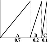
(a) Source $X$: {$A$,$B$,$C$} with probabilities {0.7, 0.2, 0.1}, $\lambda_{X}=1.156$.
       

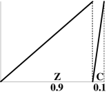
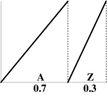
(b) $A$ and $B$ merged.                (c) $B$ and $C$ merged.
($\lambda_{AB}=0.47$)                             ($\lambda_{BC}=0.88$)

(d) $A$ and $C$ merged ($\lambda_{AC}=0.73$).

Figure 5: Successive source approximation using GLS: An example. Here, $\lambda_{BC}$ is the closest to $\lambda_{X}$. Unit of $\lambda(.)$ is bits/iteration.

III.2 Codewords are Symbolic Sequences

At the end of Algorithm 1, we have order-2 approximation ($X_{2}$). We allocate the code $C_{2}=\{0,1\}$ to the two partitions. When we go from $X_{2}$ to $X_{3}$, the two sibling partitions that were merged to form the parent partition will get the codes ‘$S0$’ and ‘$S1$’ where ‘$S$’ is the codeword of the parent partition. This process is repeated until we have allocated codewords to $X_{N}$.

It is interesting to realize that the codewords are actually symbolic sequences on the standard binary map. By allocating the code $C_{2}=\{0,1\}$ to $X_{2}$ we are essentially treating the two partitions to have equal probabilities although they may be highly skewed. In fact, we are approximating the source $X_{2}$ as a GLS with equal partitions (=0.5 each) which is the standard binary map. The code $C_{2}$ is thus the symbolic sequence on the standard binary map. Now, moving up from $X_{2}$ to $X_{3}$ we are doing the same approximation. We are treating the two sibling partitions to have equal probabilities and giving them the codes ‘$S0$’ and ‘$S1$’ which are the symbolic sequences for those two partitions on the standard binary map. Continuing in this fashion, we see that all the codes are symbolic sequences on the standard binary map. Every alphabet of the source $X$ is approximated to a partition on the binary map and the codeword allocated to it is the corresponding symbolic sequence. It will be proved that the approximation is minimum redundancy and as a consequence of this, if the probabilities are all powers of 2, then the approximation is not only minimum redundancy but also equals the entropy of the source ($L_{\mathcal{C}}(X)=H(X)$).

Theorem 2: (Successive Source Approximation) The successive source approximation algorithm using GLS yields minimum-redundancy (i.e., it minimizes $L_{\mathcal{C}}(X)$).

Proof:
We make the important observation that the successive source approximation algorithm is in fact a re-discovery of the binary Huffman coding algorithm Huffman1952 which is known to minimize $L_{\mathcal{C}}(X)$ and hence yields minimum-redundancy. Since our algorithm is essentially a re-discovery of the binary Huffman coding algorithm, the theorem is proved (the codewords allocated in the previous section are the same as Huffman codes). $\hfill\square$

III.3 Encoding and Decoding

We have described how by successively approximating the original stochastic i.i.d source using GLS, we arrive at a set of codewords for the alphabet which achieves minimum redundancy. The assignment of symbolic sequences as codewords to the alphabet of the source is the process of encoding. Thus, given a series of observations of $X$, the measuring device represents and stores these as codewords. For decoding, the reverse process needs to be applied, i.e., the codewords have to be replaced by the observations. This can be performed by another device which has a look-up table consisting of the alphabet set and the corresponding codewords which were assigned originally by the measuring device.

IV Some Remarks

We make some important observations/remarks here:

1. The faithful modeling of a stochastic i.i.d source as a GLS is a very important step. This ensured that the Lyapunov exponent captured the information content (Shannon’s Entropy) of the source.

2. Codewords are symbolic sequences on GLS. We could have chosen a different scheme for giving codewords than the one described here. For example, we could have chosen symbolic sequences on the Tent map as codewords. This would also correspond to a different set of Huffman codes, but with the same average codeword length $L_{\mathcal{C}}(X)$. Huffman codes are not unique but depend on the way we assign codewords at every level.

3. Huffman codes are symbol codes, i.e., each symbol in the alphabet is given a distinct codeword. We have investigated binary codes in this paper. An extension to the proposed algorithm is possible for ternary and higher bases.

4. In another related work, we have used GLS to design stream codes. Unlike symbol codes, stream codes encode multiple symbols at a time. Therefore, individual symbols in the alphabet no longer correspond to distinct codewords. By treating the entire message as a symbolic sequence on the GLS, we encode the initial condition which contains the same information. This achieves optimal lossless compression as demonstrated in NithinGLS .

5. We have extended GLS to piecewise non-linear, yet Lebesgue measure preserving discrete chaotic dynamical systems. These have very interesting properties (such as Robust Chaos in two parameters) and are useful for joint compression and encryption applications NithinGLS .

V Conclusions

Source coding problem is motivated as a measurement problem. A stochastic i.i.d source can be faithfully “embedded” into a piecewise linear chaotic dynamical system (GLS) which exhibits interesting properties. The Lyapunov exponent of the GLS is equal to Shannon’s entropy of the i.i.d source. The measurement problem is addressed by successive source approximation using GLS with the nearest Lyapunov exponent (by merging the two least probable states). By assigning symbolic sequences as codewords, we re-discovered the popular Huffman coding algorithm – a minimum redundancy symbol code for i.i.d sources.

References

- (1) C. E. Shannon, Bell Sys. Tech. Journal 27, 379 (1948).
- (2) D. J. C. MacKay, Information Theory, Inference and Learning Algorithms (Cambridge University Press, 2003).
- (3) W. Ebeling, and M. A. Jiménez-Montaño, Math. Biosc. 52, 53 (1980); M. A. Jiménez-Montaño, Bull. Math. Biol. 46, 641 (1984); P. E. Rapp, I. D. Zimmermann, E. P. Vining, N. Cohen, A. M. Albano, and M. A. Jiménez-Montaño, Phys. Lett. A 192, 27 (1994); M. A. Jiménez-Montaño, W. Ebeling, and T. Pöschel, preprint arXiv:cond-mat/0204134 [cond-mat.dis-nn] (2002).
- (4) P. Grassberger, preprint arXiv:physics/0207023v1 [physics.data-an], (2002).
- (5) L. M. Calcagnile, S. Galatolo, and G. Menconi, preprint arXiv:0809.1342v1 [cond-mat.stat-mech] (2008).
- (6) N. Nagaraj, P. G. Vaidya, and K. G. Bhat, Comm. in Non-linear Sci. and Num. Sim. 14, 1013 (2009).
- (7) N. Nagaraj, Chaos 19, 013136 (2009).
- (8) D. A. Huffman, in Proceedings of the I.R.E. 1952, 40(9) p. 1098.
- (9) G. K. Wallace, Comm. of the ACM 34, 30 (1991).
- (10) A. Papoulis, and S. U. Pillai, Probability, Random Variables and Stochastic Processes (McGraw Hill, New York, 2002).
- (11) T. Kohda, in Proceedings of the IEEE 2002, 90(5) p. 641.
- (12) V. S. Afraimovich, and S.-B. Hsu, Lectures on Chaotic Dynamical Systems (American Mathematical Society and International Press, 2003).
- (13) K. Dajani, and C. Kraaikamp, Ergodic Theory of Numbers (The Mathematical Association of America, Washington, DC, 2002).
- (14) M. S. Waterman, Amer. Math. Monthly 82, 622 (1975).
- (15) G. Cantor, Z. Math. und Physik 14, 121 (1869).
- (16) N. Nagaraj, and P. G. Vaidya, in Proceedings of Intl. Conf. on Recent Developments in Nonlinear Dynamics 2009, Narosa publishing house, edited by M. Daniel and S. Rajasekar (School of Physics, Bharathidasan University, 2009), p. 393; N. Nagaraj, Ph.D. thesis, National Institute of Advanced Studies 2009.