Deformable Model with a Complexity Independent from Image Resolution

Abstract

We present a parametric deformable model which recovers image components with a complexity independent from the resolution of input images. The proposed model also automatically changes its topology and remains fully compatible with the general framework of deformable models. More precisely, the image space is equipped with a metric that expands salient image details according to their strength and their curvature. During the whole evolution of the model, the sampling of the contour is kept regular with respect to this metric. By this way, the vertex density is reduced along most parts of the curve while a high quality of shape representation is preserved. The complexity of the deformable model is thus improved and is no longer influenced by feature-preserving changes in the resolution of input images. Building the metric requires a prior estimation of contour curvature. It is obtained using a robust estimator which investigates the local variations in the orientation of image gradient. Experimental results on both computer generated and biomedical images are presented to illustrate the advantages of our approach.

1 Introduction

In the field of image analysis, recovering image components is a difficult task. This turns out to be even more challenging when objects exhibit large variations of their shape and topology. Deformable models that are able to handle that kind of situations can use only little a priori knowledge concerning image components. This generally implies prohibitive computational costs (see Table 1).

In the framework of parametric deformable models, most authors [1, 2, 3] propose to investigate the intersections of the deformable model with a grid that covers the image space. Special configurations of these intersections characterize the self collisions of the mesh. Once self-instersections have been detected, local reconfigurations are performed to adapt the topology of the model according to its geometry. To take advantage of all image details, the grid and the image should have the same resolution. An other method [4] consists in constraining the lengths of the edges of the model between two bounds. Self-collisions are then detected when distances between non-neighbor vertices fall under a given threshold. Topological consistency is recovered using local operators that reconnect vertices consistently. Using all image details requires edges to have the same size as image pixels. The complexities of all these methods are thus directly determined by the size of input data.

In the framework of level-set methods, boundaries of objects are implicitly represented as the zero level set of a function $f$ [5, 6, 7, 8]. Usually $f$ is sampled over a regular grid that has the same resolution as the input image. Then $f$ is iteratively updated to make its zero level-set approach image contours. Even with optimization methods which reduce computations to a narrow band around evolving boundaries [9, 10], the complexity of these methods is determined by the resolution of the grid and hence by the resolution of the input image.

Table 1: Complexities of the deformable models that automatically adapt their topology. The length of the deformable model is denoted $l$, the with of a pixel is denoted $d$. The size of the image is denoted $|I|$, and $k$ denotes the width of the narrow band when this optimization is used. This shows that the complexities of these algorithms are completely determined by the resolution of the input image.

Model	Complexity per iteration
T-Snake[3]	$O(|I|)$
Simplex mesh[1]	$O(\frac{l}{d})$
Distance constraints[4])	$O(\frac{l}{d}\log\left(\frac{l}{d}\right))$
Level-set [5, 7]	$O(|I|)$
Level-set with narrow band [9]	$O\left(k\frac{l}{d}\right)+0\left(\frac{l}{d}\log\left(\frac{l}{d}\right)\right)$

In [11] a method is proposed to adapt the resolution of a deformable model depending on its position and orientation in the image. The main idea is to equip the image space with a Riemannian metric that geometrically expands parts of the image with interesting features. During the whole evolution of the model, the length of edges is kept as uniform as possible with this new metric. As a consequence, a well chosen metric results in an accuracy of the segmentation process more adapted to the processed image.

In this first attempt the metric had to be manually given by a user. This was time consuming and the user had to learn how to provide an appropriate metric. Our contribution is to propose an automated way of building metrics directly from images. The accuracy of the reconstruction is determined by the geometry of image components. The metric is built from the image

1. to optimize the number of vertices on the final mesh, thus enhancing the shape representation,

2. and to reduce both the number and the cost of the iterations required to reach the rest position.

Property (1) is obtained by building the metric in such a way that the length of the edges of the model linearly increases with both the strength and the radius of curvature of the underlying contours.

Property (2) is ensured by designing the metric in such a way that a coarse sampling of the curve is kept far away from image details, while it progressively refines when approaching these features.

To build a metric which satisfies these constraints, the user is asked for only three parameters:

• $s_{\text{ref}}$: the norm of the image gradient over which a contour is considered as reliable,

• $l_{\text{max}}$: the maximum length of the edges of the deformable model (this is required to prevent edges from growing too much which would lead to numerical instability),

• $l_{\text{min}}$: the minimum length of an edge (typically this corresponds to the half width of a pixel).

Over a sufficient resolution of the input image, the gradient magnitude as well as the curvature of objects do not depend on the sampling rate of the input image. Consequently the computational complexity of the segmentation algorithm is determined only by the geometrical complexity of image components and no longer by the size of input data.

The dynamics of the deformable model is enhanced too. In places without image structures the length of edges reaches its maximum. This results in (i) less vertices and (ii) larger displacements of these vertices. By this way both the cost per iteration and the number of iterations required to reach convergence are reduced.

We point out that these enhancements do not prevent the model from changing its topology and that the complexity of these topology changes is determined by the (reduced) number of vertices. Other methods, such as those presented in [1] and [3] require the model to be resampled (at least temporarily) on the image grid. As a result, these methods cannot take advantage of better sampling of the deformable curve to reduce their complexity.

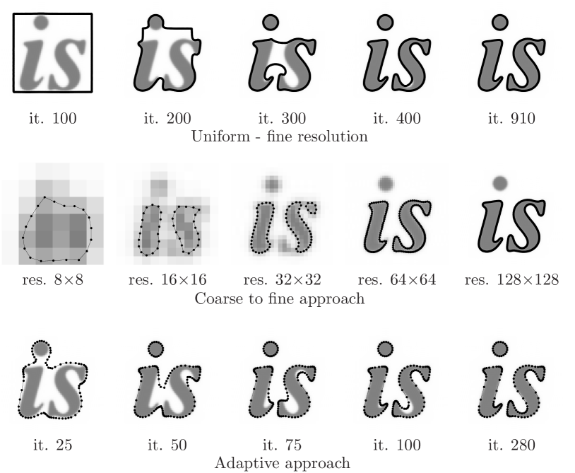
Fig. 1 illustrates the main idea of our approach and offers a comparison with the classical snake approach and with a coarse-to-fine snake method. Note that the same parameters are used for all three experiments: force coefficients, initialization, convergence criterion. First, it appears clearly that our approach achieves the same segmentation quality as regular snakes with a high precision. A coarse-to-fine approach may fail to recover small components. Second, computation times are greatly improved with our approach (about 6 times faster). The coarse-to-fine approach is also rather slow since a lot of time is spent extracting details that were not present at a coarser level. Third, the number of vertices is optimized according to the geometry of the extracted shape (3 times less vertices).

Moreover, the proposed model remains compatible with the general framework of deformable models: to enhance the behavior of the active contour, any additional force [12, 13, 14] may be used without change. In practice, with the same sets of forces, the visual quality of the segmentation is better with an adaptive vertex density than in the uniform case. Indeed, along straight parts of image components, the slight irregularities that result from the noise in the input images are naturally rubbed out when fewer vertices are used to represent the shape. In the vicinity of fine image details an equivalent segmentation accuracy is achieved in both the adaptive and uniform cases.

At last, the approach proposed to build the metric is almost fully automated. Thus, only little user interaction is required. However it remains easy to incorporate additional expert knowledges to specify which parts of image components have to be recovered accurately.

This paper is structured as follows: in Sect. 2 we describe the proposed deformable model and we show how changing metrics induces adaptive resolution. In Sect. 3, we explain how suitable metrics are built directly from images using a robust curvature estimator. Experimental evaluation of both the proposed model and the curvature estimator are presented in Sect. 4.

Figure 1: Illustration of the proposed approach to shape extraction. Top row: extraction with uniform sampling of the model. The edge length has approximately the pixel width. Computation statistics: 910 iterations, 10.14s, 458 vertices. Middle row: coarse to fine extraction. At each level, the edge length has approximately the pixel width. Computation statistics: 310+810+760+1020+510 iterations, 9.23s = 0.08+0.40+0.87+3.10+4.78, 392 vertices. Bottom row: extraction with adaptive sampling of the model. The edge length varies between half the pixel width and 20 times the pixel width. Computation statistics: 280 iterations, 1.73=0.31+1.42s (precomputation + evolution), 150 vertices.

2 Deformable Model

2.1 General description

Our proposed deformable model follows the classical energy formulation of active contours [15]: it is the discretization of a curve that is emdedded in the image space. Each of its vertices undergoes forces that regularize the shape of the curve, attract them toward image features and possibly tailor the behavior of the model [12, 13] for more specific purposes. In this paper, classical parametric snakes are extended with the ability to (i) dynamically and automatically change their topology in accordance with their geometry and (ii) adapt their resolution to take account of the geometrical complexity of recovered image components. In addition, only little work is necessary to adapt the proposed model for three-dimensional image segmentation (see [16] for details). In this three dimensional context, the number of vertices is further reduced and computation times are consequently greatly improved.

2.2 Resolution adaptation

During the evolution of the model, the vertex density along the curve is kept as regular as possible by constraining the length of the edges of the model between two bounds $\delta$ and $\zeta\delta$:

$$\delta\leq L_{E}(u,v)\leq\zeta\delta\mbox{ ,}$$ (1)

In (1) $L_{E}$ denotes the length of the line segment that joins $u$ and $v$. The parameter $\delta$ determines lengths of edges and hence vertex density along the curve. The parameter $\zeta$ determines the allowed ratio between maximum and minimum edge lengths.

At every step of the evolution of the model, each edge is checked. If its length is found to be less than $\delta$ then it is contracted. In contrast, if its length exceeds the $\zeta\delta$ threshold then the investigated edge gets split. To ensure the convergence of this algorithm $\zeta$ must be chosen greater than two. In the following $\zeta$ is set to the value $2.5$, which provides satisfying results in practice. The parameter $\delta$ is derived from the maximum edge length $l_{\text{max}}$ specified by the user as $\delta=l_{\text{max}}/\zeta$.

Adaptive resolution is achieved by replacing the Euclidean length estimator $L_{E}$ by a position and orientation dependent length estimator $L_{R}$ in (1). In places where $L_{R}$ underestimates distances, estimated lengths of edges tend to fall under the $\delta$ threshold. As a consequence, edges tend to contract and the resolution of the model locally decreases. In contrast, the resolution of the model increases in regions where $L_{R}$ overestimates distances.

More formally, Riemannian geometry provides us with theoretical tools to build such a distance estimator. In this framework, the length of an elementary displacement $\mathbf{ds}$ that starts from point $(x,y)$ is expressed as:

$$\|\mathbf{ds}\|_{R}^{2}={\vphantom{\mathbf{ds}}}^{t}{\mathbf{ds}}\times G(x,y)\times\mathbf{ds},$$ (2)

where $G$ associates a positive-definite symmetrical matrix with each point of the space. The $G$ mapping is called a Riemannian metric. From (2) follow the definitions of the Riemannian length of a path as

$$L_{R}(\gamma)=\int_{a}^{b}\|\mathbf{\dot{\gamma}}(t)\|_{R}\;dt\mbox{ ,}$$ (3)

and of the Riemannian distance between two points $u$ and $v$ as

$$d_{R}(u,v)=\inf_{\gamma\in{\mathcal{C}}}L_{R}(\gamma)\mbox{ ,}$$ (4)

where ${\mathcal{C}}$ contains all the paths that join $u$ and $v$. It is thus easily seen that defining the $G$ mapping is enough to completely define our new length estimator $L_{R}$. How this mapping is built from images to enhance and speed up shape recovery is discussed in Sect. 3.

2.3 Topology adaptation

During the evolution of the model, care must be taken to ensure that its interior and exterior are always well defined: self-collisions are detected and the topology of the model is updated accordingly (see [11] for more details on topology adaptation).

Since all the edges have their length lower than $\zeta\delta$, a vertex that crosses over an edge $(u,v)$ must approach either $u$ or $v$ closer than $\frac{1}{2}(\zeta\delta+d_{max})$, where $d_{max}$ is the largest distance covered by a vertex during one iteration. Self-intersections are thus detected by looking for pairs of non-neighbor vertices $(u,v)$ for which

$$d_{E}(u,v)\leq\frac{1}{2}(\zeta\delta+d_{max})\mbox{ .}$$ (5)

It is easily shown that this detection algorithm remains valid when $d_{E}$ is replaced with a $d_{R}$ distance estimator as described in Sect. 2.2. With a naive implementation, the complexity of this method is quadratic. However, it is reduced to $O(n\log n)$ by storing vertex positions in an appropriate quadtree structure.

Detected self-intersections are solved using local operators that restore a consistent topology of the mesh by properly reconnecting the parts of the curve involved in the collision.

2.4 Dynamics

Theoretically, in a space equipped with a Riemannian metric, the position $\mathbf{x}$ of a vertex that undergoes a force $\mathbf{F}$ follows equation

$$m\ddot{x}_{k}=F_{k}-\sum_{i,j}\Gamma_{ij}^{k}\dot{x}_{i}\dot{x}_{j}\mbox{ ,}$$ (6)

where the $\Gamma_{ij}^{k}$ coefficients are known as the Christoffel’s symbols associated with the metric:

$$\Gamma_{ij}^{k}=\frac{1}{2}\sum_{k}g^{kl}\left(\frac{\partial g_{il}}{\partial x_{j}}+\frac{\partial g_{lj}}{\partial x_{i}}-\frac{\partial g_{ij}}{\partial x_{l}}\right)\mbox{ .}$$ (7)

However, the last term of (6) is quadratic in $\mathbf{\dot{x}}$ and has therefore only little influence when the model is evolving. Furthermore, once at rest position it cancels and has consequently no impact on the final shape. Therefore it is neglected and we get back the classical Newton’s laws of motions. Experimentally, removing this term does not induce any noticeable change in the behavior of the model.

3 Tailoring Metrics to Images

3.1 Geometrical interpretation

For any location $(x,y)$ in the image space, the metric $G(x,y)$ is a positive-definite symmetrical matrix. Thus, in an orthonormal (for the Euclidean norm) base $(\mathbf{v}_{1},\mathbf{v}_{2})$ of eigenvectors, $G(x,y)$ is diagonal with coefficients $(\mu_{1},\mu_{2})$. Hence, the length of an elementary displacement $\mathbf{ds}=x_{1}\mathbf{v}_{1}+x_{2}\mathbf{v}_{2}$ is expressed as

$$\|\mathbf{ds}\|_{R}^{2}=\mu_{1}x_{1}^{2}+\mu_{2}x_{2}^{2}\mbox{ .}$$ (8)

This shows that changing the Euclidean metric with a Riemannian metric locally expands or contracts the space along $\mathbf{v}_{1}$ and $\mathbf{v}_{2}$ with ratios $1/\sqrt{\mu_{1}}$ and $1/\sqrt{\mu_{2}}$. Suppose now that $L_{E}$ replaced by $L_{R}$ in (1). In a place where the edges of the model are aligned with $\mathbf{v}_{1}$ this yields

$$\frac{\delta}{\sqrt{\mu_{1}}}\leq L_{E}(e)\leq\frac{\zeta\delta}{\sqrt{\mu_{1}}}\mbox{ .}$$ (9)

Of course a similar inequality holds in the orthogonal direction. This shows that (from a Euclidean point of view) the vertex density on the mesh of the model is increased by a ratio $\sqrt{\mu_{1}}$ in the direction of $\mathbf{v}_{1}$ and by a ratio $\sqrt{\mu_{2}}$ in the direction of $\mathbf{v}_{2}$. Therefore, at a given point of the image space, a direct control over the vertex density on the deformable mesh is obtained by properly tweaking $\mathbf{v}_{1}$, $\mathbf{v}_{2}$, $\mu_{1}$ and $\mu_{2}$ in accordance with underlying image features.

Although these eigenvectors and eigenvalues could be given by a user, it is a tedious and complicated task. It is therefore much more attractive and efficient to have them selected automatically. The subsequent paragraphs discuss this problem and describe a method to build the metric directly from the input image in such a way that the vertex density of the mesh adapts to the geometry of image components and no longer depends on the resolution of input data.

This property is interesting because the model complexity is made independent from the image resolution and is defined instead only by the geometrical complexity of the object to recover. Now, the geometrical complexity of an object embedded in an image cannot exceed the image resolution. Furthermore, since objects do not have high curvatures everywhere on their boundary, this complexity is generally much smaller.

3.2 Definition of metrics

Two cases have to be considered:

1. the case for which the model has converged, and for which we expect it to follow image contours,

2. and the case for which the model is still evolving. Thus parts of the curve may be far away of image details or cross over significant contours.

In case 1, the length of its edges is determined by (i) the geometrical properties of the recovered image components and (ii) the certainty level of the model position. More precisely, the length of edges is an increasing function of both the strength and curvature of the underlying contours.

In case 2, two additional sub-cases are possible.

• If the model crosses over the boundary of image components, the vertex density on the curve is increased. By this way the model is given more degrees of freedom to get aligned with the contour.

• In a place with no image feature (i.e. far away from image contours) vertex density is kept as low as possible. As a consequence, the number of vertices and hence the computational complexity decreases. Moreover since edge length is increased, vertices are allowed to travel faster. The number of iterations required to reach the rest position of the model is thus reduced.

To obtain these properties, the eigenstructure of the metric is chosen as follows

$$\left\{\begin{array}[]{lcl}\mathbf{v}_{1}=\mathbf{n}&\;\mbox{and}&\mu_{1}=\left[\displaystyle\frac{s^{2}}{{s_{\text{ref}}}^{2}}\times\frac{{\kappa_{\text{max}}}^{2}}{{\kappa_{\text{ref}}}^{2}}\right]_{1,\frac{{\kappa_{\text{max}}}^{2}}{{\kappa_{\text{ref}}}^{2}}}\\ \mathbf{v}_{2}=\mathbf{n}^{\bot}&\;\mbox{and}&\mu_{2}=\left[\displaystyle\frac{\kappa^{2}}{{\kappa_{\text{max}}}^{2}}\times\mu_{1}\right]_{1,{\mu_{1}}}\end{array}\right.\mbox{ ,}$$ (10)

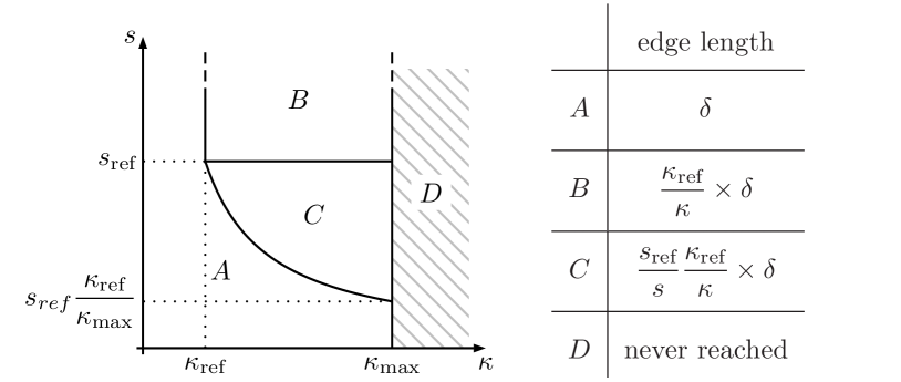
where $\mathbf{n}$ denotes a vector normal to the image contour, and the notation $[\cdot]_{a,b}$ constrains its arguments between the bounds $a$ and $b$. The parameters $s$ and $\kappa$ respectively denote the strength and the curvature of contours at the investigated point of the image. The parameter $\kappa_{\text{max}}$ corresponds to the maximum curvature that is detected in the input image. The different possible situations are depicted on Fig. 2. Computing these parameters directly from images is not straightforward and is discussed in Sect. 3.4.

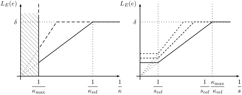
The parameter $s_{\text{ref}}$ is user-given. It specifies the strength over which a contour is assumed to be reliable. If an edge runs along a reliable contour, then its length is determined only by the curvature of the contour (see region $B$ in Fig. 2 and Fig. 3-left). In other cases the length of edges decreases as the contour gets weaker.

The parameter $\kappa_{\text{ref}}$ is a reference curvature for which the length of edges is allowed to vary between $\delta$ and $\zeta\delta$ only. Below this curvature contours are assumed to be straight and the length of edges remains bounded between $\delta$ and $\zeta\delta$. Along more curved contours, the length of edges increases linearly with the radius of curvature (see Fig. 3-left). This parameter is easily computed from the minimal length allowed by the user for the edges (see Fig. 2):

$$\frac{\kappa_{\text{ref}}}{\kappa_{\text{max}}}\delta=l_{\text{min}}\mbox{,}$$ (11)

where $l_{\text{min}}$ denotes the chosen minimal length. To take advantage of all the details available in the image, it is usual to set $l_{\text{min}}$ to the half width of a pixel.

Note that all the parameters are squared to compensate for the square root in (9). By this way the length of edges varies linearly with both $1/s$ and $1/k$.

Figure 2: Edge length (up to a factor at most $\zeta$) depending on the strength $s$ and curvature $\kappa$ of the underlying contour. It is assumed that edges run along the contour. In region $A$ contours are too weak or too straight. Therefore, edges keep their maximum length. In region $B$ contours are considered as reliable and have a curvature higher than the reference curvature $\kappa_{\text{ref}}$. The length of the edges increases linearly with the radius of curvature of underlying contours. In region $C$ contours have a varying reliability and have a curvature higher than the reference curvature. The length of edges depends on both $s$ and $\kappa$. The separation between regions $A$ and $C$ corresponds to contours for which $\frac{\kappa}{\kappa_{\text{ref}}}\frac{s}{s_{\text{ref}}}=1$. It corresponds to contours for which curvature and/or strength fall too low to let the model increase its vertex density safely.

Figure 3: Left: edge length (up to a $\zeta$ factor) as a function of the radius of curvature of the underlying contour. The solid line corresponds to a reliable contour ($s\geq s_{\text{ref}}$), the dashed line corresponds to a weaker contour ($s\leq s_{\text{ref}}$). The hatched part of the graph cannot be reached since estimated curvatures cannot exceed $\kappa_{\text{max}}$. Right: edge length (up to a factor at most $\zeta$) as a function of the strength of the underlying contour. The solid line corresponds to a contour with the highest possible curvature ($\kappa=\kappa_{\text{max}}$). The dashed lines corresponds to less curved contours ($\kappa\leq\kappa_{\text{max}}$). In both figures, it is assumed that edges run along the contour.

3.3 Influence of the resolution of input images

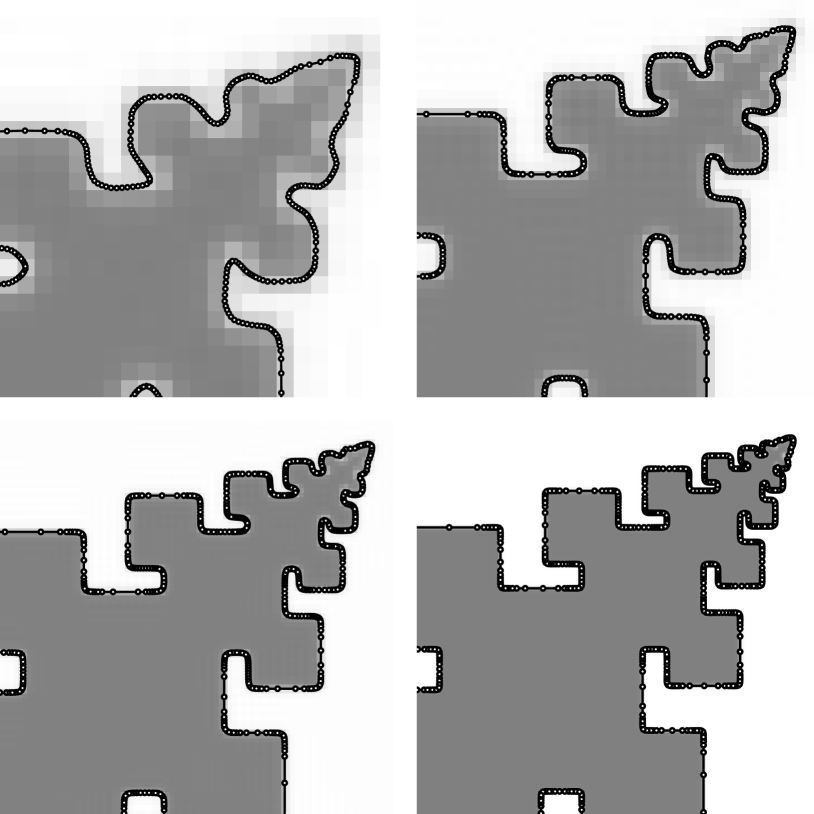
For input images with sufficiently high sampling rates, both $s$ and $\kappa$ are determined only by the geometry of image components. Consequently, the vertex density during the evolution of the model and after convergence are completely independent from the image resolution (see experimental results on Fig. 10).

If the sampling rate is too low to preserve all the frequencies of objects, contours are smoothed and fine details may be damaged. As a result, $s$ is underestimated over the whole image and $\kappa$ along highly curved parts of objects. In these areas, the insufficient sampling rate induces longer edges and details of objects cannot be represented accurately. However, these fine structures are not represented in input images. As a consequence, it is not worth increasing the vertex density since small features cannot be recovered even with shorter edges.

In featureless regions, or along straight object boundaries, the length of the edges depend neither on $s$ nor on $\kappa$ and remains bounded between $\delta$ and $\zeta\delta$ (see Fig. 2). As a result the improper sampling rate of the image has no impact on the vertex density on the deformable curve in these regions, which remains coarse.

As a result of this behavior, the segmentation process is able to take advantage of all finest details that can be recovered in the image. Indeed, when the resolution of the input image is progressively increased, contours and details are restored and $s$ and $\kappa$ get back their actual value. As a consequence the lengths of edges progressively decrease in image parts with fine details while remaining unchanged elsewhere. At the same time the global complexity of the model increases only slightly with the resolution of images until all the frequencies of image components are recovered. If the image is oversampled, $s$ and $\kappa$ are left invariant, and the number of vertices, and hence the complexity remains unaffected.

These properties are illustrated experimentally on Fig. 10, Fig. 11 and 12.

3.4 Computing strength and curvature of contours from images

To tailor metrics to enhance and fasten image segmentation we need to estimate both the strength $s$ of image contours and their curvature $\kappa$.

Consider a unit vector $\mathbf{v}$ and $Q_{\mathbf{v}}(x,y)=(\mathbf{v}\cdot\mathbf{\nabla I}(x,y))^{2}$. This quantity reaches its maximum when $\mathbf{v}$ has the same orientation (modulo $\pi$) as $\mathbf{\nabla I}(x,y)$. The minimum is reached in the orthogonal direction. To study the local variations of the image gradient it is convenient to consider the average of $Q_{\mathbf{v}}$ over a neighborhood. It is expressed in a matrix form as

$$\overline{Q_{\mathbf{v}}}(x,y)={\vphantom{\mathbf{v}}}^{t}{\mathbf{v}}\times\overline{\mathbf{\nabla I}\times{\vphantom{\mathbf{\nabla I}}}^{t}{\mathbf{\nabla I}}}\times\mathbf{v}\mbox{ ,}$$ (12)

where $\overline{(\cdot)}$ denotes the average of its argument over a neigborhood of point $(x,y)$. The positive-definite symmetrical matrix $J=\overline{\mathbf{\nabla I}\times{\vphantom{\mathbf{\nabla I}}}^{t}{\mathbf{\nabla I}}}$ is known as the gradient structure tensor. This operator is classically used to analyze local structures of images [17], since it characterizes their local orientations. It is further used for texture and image enhancement in anisotropic diffusion schemes [18, 19].

Let $\left\{(\mathbf{w}_{1},\xi_{1}),(\mathbf{w}_{2},\xi_{2})\right\}$ denote the eigen decomposition of $J$ and assume that $\xi_{2}\leq\xi_{1}$. It is easily seen that $\xi_{1}$ and $\xi_{2}$ respectively correspond to the maximum and minimum values reached by $Q_{\mathbf{v}}$ when the unit vector $\mathbf{v}$ varies. Eigenvectors indicate the directions for which these extrema are reached. Thus, they respectively correspond to the average direction of image gradients over the investigated neighborhood and to the orthogonal direction. The eigenvalues $\xi_{1}$ and $\xi_{2}$ store information on the local coherence of the gradient field in the neighborhood. When $\overline{(\cdot)}$ is implemented as a convolution with a Gaussian kernel $g_{\rho}$ ($\rho$ corresponds the size of the investigated neighborhood), the eigenvalues can be combined as follows to build the required estimators $s$ and $\kappa$:

$$\left\{\begin{array}[]{l}s^{2}\simeq\xi_{1}+\xi_{2}={\mathrm{Tr}}(J)=g_{\rho}\ast\left(\|\mathbf{\nabla I}\|^{2}\right)\\ \displaystyle\kappa^{2}\simeq\frac{1}{\rho^{2}}\times\frac{\xi_{2}}{\xi_{1}}\end{array}\right.\mbox{ .}$$ (13)

The estimator $s$ is approximately equivalent to the average norm of the gradient. The curvature estimator is based on a second order Taylor expansion of $I$ along a contour. With this approximation the eigenvalues of the structure tensor can be expressed as functions of the strength and the curvature of contours. The curvature $\kappa$ is then easily extracted (see Appendices for more details).

4 Experiments

4.1 Quality of the curvature estimator

This section illustrates the accuracy and robustness of our proposed curvature estimator. We investigate the influence of the sizes of the Gaussian kernels used to compute the gradient structure tensor and we compare our estimator with previous works.

For this purpose, we generate images of ellipses with known curvature. These images are corrupted with different levels of Gaussian noise (see Fig. 4). Then curvature is computed along ellipses with our estimator and results are compared with the true curvature. For a given noise level, the experiment is repeated $40$ times. The presented curves show the averages and the standard deviations of estimated curvatures over this set of $40$ test images. Noise levels are expressed using the peak signal to noise ratio defined as $PSNR=10\log\frac{I_{\text{max}}}{\sigma}$ where $I_{\text{max}}$ is the maximum amplitude of the input signal and $\sigma$ is the standard deviation of the noise.

Fig. 5 illustrates the influence of the parameter $\sigma$. As expected, it must be chosen in accordance with the noise level in the image. If $\sigma$ is too small, the direction of the image gradient changes rapidly in a neighborhood of the considered point. As a consequence, the second eigenvalue of the structure tensor increases. This explains why curvature is overestimated.

The dependency of our estimator on the radius $\rho$ of the local integration is depicted on Fig. 6. The presented curves show that this parameter has an influence only for images with strong noise. Indeed, contour information has to be integrated over much larger neighborhoods to mitigate the influence of noise.

In addition, our estimator is compared with two methods which both involve the computation of the second derivatives of the input image:

• the naive operator which simply computes the curvature of isocontours of the image as

  $$\kappa=\mathrm{div}\left(\frac{\mathbf{\nabla I}}{\|\mathbf{\nabla I}\|}\right)=\frac{I_{xx}{I_{y}}^{2}-2I_{xy}I_{x}I_{y}+I_{yy}{I_{x}}^{2}}{\left({I_{x}}^{2}+{I_{y}}^{2}\right)^{\frac{3}{2}}}\mbox{ ,}$$ (14)

• the more elaborate estimator proposed by Rieger et al. [20].

The latter method consists in computing the derivative of the contour orientation in the direction of the contour. Contour orientation is computed (modulo $\pi$) as the eigenvector $\mathbf{w}_{1}$ of the gradient structure tensor (which corresponds to the largest eigenvalue). Since orientation is only known modulo $\pi$, the vector $\mathbf{w}_{1}$ is converted into an appropriate continuous representation (using Knutsson mapping) prior to differentiation.

As shown on Fig. 7 all these estimators provide fairly equivalent results along a contour. Note however that the naive estimator is much more sensitive to noise than the others.

These estimators were also tested in places without image features. As depicted on Fig. 8, both the naive estimator and the one of Rieger et al. become unstable. The naive estimator fails because the denominator in (14) falls to zero and because second derivatives are very sensitive to noise. Rieger’s method can neither be used. Indeed, in a region without significant contour, the eigenvector $\mathbf{w}_{1}$ of the gradient structure tensor is only determined by noise and thus exhibits rapid variations. Computing its derivatives results in a spurious evaluation of the curvature. This justifies the use of our estimator, which, in addition, requires less computations than Rieger’s method since it estimates curvature directly from the eigendecomposition of the gradient structure tensor and does not involve their derivatives.

Figure 4: Images used to test curvature estimators (from left to right $PSNR=40\;\mathrm{dB}$, $30\;\mathrm{dB}$ and $20\;\mathrm{dB}$). The curvature is estimated along the border of ellipses and are compared with the true curvature for different estimators and different values of the parameters. Results are presented on Fig. 5-7.

Figure 5: Estimated curvature as a function of the true curvature for different values of $\sigma$ and for $\rho=10$ (the x-axis and y-axis respectively correspond to the true and estimated curvatures). The three graphics correspond to different noise levels: $PSNR=40\;\mathrm{dB}$ (top-left), $PSNR=30\;\mathrm{dB}$ (top-right) and $PSNR=20\;\mathrm{dB}$ (bottom).

Figure 6: Estimated curvature as a function of the true curvature for $\sigma=5$ and for different values of $\rho$ (abscissa and ordinate respectively correspond to the true and estimated curvatures). The three graphics correspond to different noise levels: $PSNR=40\;\mathrm{dB}$ (top-left), $PSNR=30\;\mathrm{dB}$ (top-right) and $PSNR=20\;\mathrm{dB}$ (bottom).

Figure 7: Comparison of curvature estimators along the contour of a noisy ellipse (left $PSNR=40\;\mathrm{dB}$, right $PSNR=20\;\mathrm{dB}$). (A) our estimator, (B) Rieger’s estimator, (C) naive estimator.

Figure 8: Comparison of curvature estimators. Left: test image ($PSNR=40\;\mathrm{dB}$). Right: curvature estimated along the radius drawn on the left figure. (A) our estimator, (B) Rieger’s estimator. The solid line represents the inverse of the distance to the center of the circle and the arrow indicates the position of the contour. The naive operator is not displayed since it is too unstable.

4.2 Parameter selection for a new image segmentation

Given a new image, we have to adjust some parameters to exploit at best the potentialies of the proposed approach. We follow the steps below:

1. The image structure tensor is computed: it provides the contour intensities $s$, the curvatures $k$ and the local metrics; the maximal curvature $k_{\text{max}}$ as well as the maximal intensity $s_{\text{max}}$ follow immediately.

2. The user chooses the minimal and the maximal edge lengths $l_{\text{min}}$ and $l_{\text{max}}$ for the model. Typically, the length $l_{\text{min}}$ is half the size of a pixel (a better precision has no sense given the input data) and the length $l_{\text{max}}$ is about 50 times $l_{\text{min}}$ for real data.

3. The user then selects the reference contour intensity $s_{\text{ref}}$ which corresponds to reliable contours. A simple way is to visualize the thresholding of the image $s$ by the value $s_{\text{ref}}$, and to tune this parameter accordingly. It can also be automated for certain images as a percentage of $s_{\text{max}}$ (typically $90\%$).

4. After that, the procedure is the same as for classical snakes: initialisation, selection of energy/force parameters, evolution until rest position.

From the preceding paragraphs, it is clear that the proposed approach does not induce significantly more interaction compared with classical snakes.

4.3 Behaviour of the deformable model

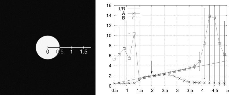
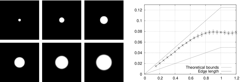
Adaptive vertex density is illustrated in Fig. 9. In this experiment images of circles with known radii are generated (left part of the figure). For each circle, the image space is equipped with a metric which is built as explained in Sect. 3. In this example $\kappa_{\text{ref}}=1$ and $s_{\text{ref}}$ is computed from the input image as the maximum value of $s$ over the image. Our deformable model is then used to segment and reconstruct the circles. Once it has converged, the Euclidean lengths of its edges are computed. The results are presented on the curve in the right part of the figure. They correspond to the expected behavior (see Fig. 3).

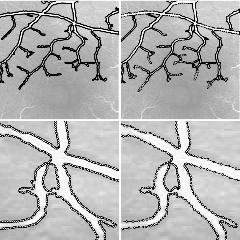
Adaptive vertex density is also visible in Fig. 11-14. As expected, changing the metric increases vertex density along highly curved parts of image components. As a result, the description of the shape of objects is enhanced while the number of vertices is optimized.

Independence with respect to the resolution of input images is shown on Fig. 10. Our model was tested on images of objects sampled at different rates (see Fig. 11). As expected, the number of vertices is kept independent from the resolution of the input image, as far as the sampling rate ensures a proper representation of the highest frequencies present in the signal. If this condition is not satisfied, as on Fig. 12, the model uses only the available information. If the resolution is increased, the length of the edges of the model remain unchanged, except in parts where the finer sampling rate of the image allows to recover finer features.

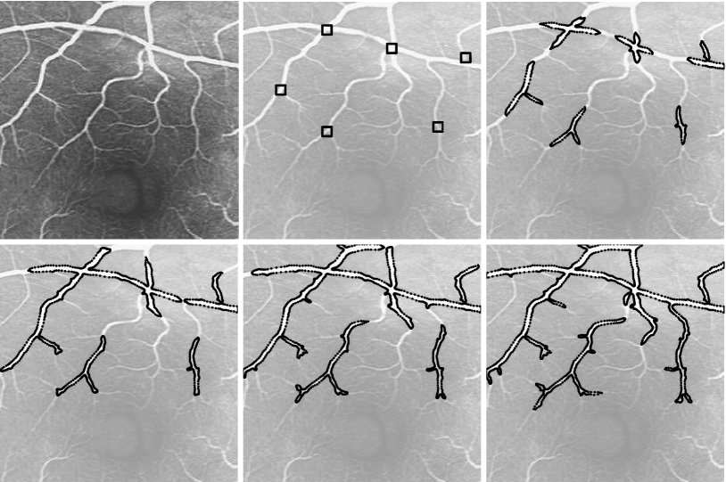
Fig. 11 and Fig. 13 demonstrate the ability of our model to dynamically and automatically adapt its topology. Note that the proposed way to build the metric is especially well suited to objects with thin and elongated features. With previous approaches [1, 2] automated topology changes can only be achieved using grids with a uniform resolution determined by the thinest part of objects. Their complexities are thus determined by the size of the smallest features to be reconstructed. The involved computational effort is therefore wasteful since much more vertices are used than required for the accurate description of objects. In contrast, replacing the Euclidean metric with a metric designed as described in this paper virtually broaden thin structures. As a consequence, even for large values of $\delta$, the inequality (5) where $d_{E}$ has been replaced by $d_{R}$ is not satisfied for two vertices $u$ and $v$ located on opposite sides of long-limbed parts of image components. Self-collisions are thus detected only where they really occur. At the same time, the number of vertices is kept independent from the size of the finest details to be recovered.

Fig. 13-14 illustrate the behavior of our deformable model on biomedical images. The input image (Fig. 13 top-right) is a fluorescein angiogram that reveals the structure of the circulatory system of the back of an eye. In addition to the classical regularizing forces, the vertices of the active contour undergo an application-specific force designed to help recovering blood vessels. This force pushes vertices in the direction of the outer normal and stops when the local gray level of the image falls under the average gray level over a neighborhood. More formally, the force $\mathbf{F}_{v}$ undergone by a vertex $v$ is defined as

$$\mathbf{F}_{v}=\left(I(v)-(g_{\tau}\ast I)(v)\right)\times\mathbf{n}_{v}\mbox{ .}$$ (15)

where $I$ is the input image, $g_{\tau}$ is a Gaussian filter used to estimate the average gray level over a neighborhood, and $\mathbf{n}_{v}$ is the outer normal to the deformable curve at vertex $v$. The presented results demonstrate the possibility to use additional forces designed to extend or improve deformable models [13, 12, 14]. Furthermore, computation times are given in Table 2. They show that reducing the number of required iterations and the number of vertices largely compensate for the time used to compute of the metric. These computation times are given in Table 3 for different size of input images.

At last, since the space is expanded only in the vicinity of image contours, vertices travel faster in parts of the image without feature. When approaching object boundaries, the deformable curve propagates slower and progressively refines. The advantage is twofold. First, the number of iterations required for the model to reach its rest position is reduced. Second, the cost of an iteration is reduced for parts of the deformable curve far away from image features, namely parts with a low vertex density. By this way a lot of computational complexity is saved when the deformable model is poorly initialized. This is especially visible on Fig. 11 (right) where the position of the model has been drawn every 50 iterations.

Figure 9: Left: test images (circles with known radii). Right: edge length as a function of the radius of curvature. Dashed lines correspond to the theoretical bounds.

Figure 10: Final number of vertices on the curve depending on the resolution of input image. The segmentation/reconstruction results as well as the evolution of the model are shown on Fig. 11.

Figure 11: Left, center: reconstruction of identical objects sampled at resolutions 40$\times$40 and 100$\times$100. Right: evolution of the deformable model every 50 iterations. The outer square corresponds to the initial position of the model.

Figure 12: Segmentation/Reconstruction of the same object sampled at increasing resolutions (50$\times$50, 100$\times$100, 200$\times$200 and 400$\times$400). For the four images all the parameters used to build the metric or attract the model toward object boundaries are identical. Please note that the deformable model automatically adapts its resolution to represent available image features as well as possible, while optimizing the number of vertices.

Figure 13: Segmentation process on an angiography. Top-left: input image. Other images: steps of the evolution of the deformable curve. The model is driven by an inflation force which stops when the local gray level is lower that the average gray-level in a neighborhood. Please note the topology changes when parts of the deformable curve collide. Computation times are given on Table 2

Figure 14: Segmentation of the angiography shown on Fig. 13. Left: results without adaptation. Right: results with a metric built as described in 3. Top: final result. Bottom: detailed view in a region which exhibits much adaptation of the vertex density as well as a complex topology. Please note how the length of edges is adapted according to the structures found in the input image and how this enables the deformable model to enter small gaps and recover structures finer than its edges. Computation times are given in Table 2.

Table 2: Number of iterations and time required to reach convergence. The table also indicates how many vertices are used to represent the whole shapes shown in Fig. 14. The two last columns describe the minimum and maximum length (in pixels) of an edge of the deformable model.

	iterations	total time (s)	vertices	min. edge length	max. edge length
uniform	350	78.5	3656	0.5	1.25
adaptive	250	37.35 (+1.24)	2065	0.35	25

Table 3: Computation times required to build the metric for different sizes of input images.

resolution of input image	100	150	200	250	300	350	400
computation time (s)	0.16	0.36	0.65	1.00	1.45	1.98	2.58

5 Conclusion

We presented a deformable model that adapts its resolution according to the geometrical complexity of image features. It is therefore able to recover finest details in images with a complexity almost independent from the size of input data. Admittedly, a preprocessing step is required to build the metric. However, involved computational costs are negligible and, as a byproduct, these precomputations provide a robust gradient estimator which can be used as a potential field for the deformable model. Most of the material used in our presented deformable model has a straightforward extension to higher dimensions [16, 21]. We are currently working on the extension of the whole approach to 3D images.

Appendix A Second order approximation of contours

In this section, we consider a contour that is tangent to the $x$ axis at the origin. This is expressed as $I_{x}(0,0)=0$ and $I_{y}(0,0)=s$, where $I_{x}$, $I_{y}$ and $s$ denote the partial derivatives of $I$ and the strength of the contour.

From the definition of a contour as a maximum of the norm of the gradient in the gradient direction follows $\left.\frac{\partial\left(\|\mathbf{\nabla I}\|\right)}{\partial\mathbf{\nabla I}}\right|_{(0,0)}=0$. Once expanded, this leads to $I_{yy}(0,0)=0$.

Let $\mathbf{t}$ and $\mathbf{n}$ denote the vectors tangent and normal to the investigated contour: $\mathbf{n}=\frac{\mathbf{\nabla I}}{\|\mathbf{\nabla I}\|}$ and $\mathbf{t}=\mathbf{n}^{\bot}$. From the definition of curvature follows $\frac{\partial\mathbf{n}}{\partial\mathbf{t}}=\kappa\mathbf{t}$. Replacing $\mathbf{t}$ and $\mathbf{n}$ by their expression as functions of $I$, and then expanding and evaluating this expression at point $(0,0)$ yields $I_{xx}(0,0)=s\kappa$.

From the above statements we get a second order Taylor expansion of $I$ as

$$I(x,y)-I(0,0)=s\left(y+\frac{1}{2}\kappa x^{2}\right)+I_{xy}xy+o(x^{2},y^{2})\mbox{ .}$$ (16)

In addition, if we assume that the strength of the contour remains constant along the contour, we get $\left.\frac{\partial\left(\|\mathbf{\nabla I}\|\right)}{\partial\mathbf{\nabla I}^{\bot}}\right|_{(0,0)}=0$. Expanding the previous expression leads to $I_{xy}(0,0)=0$.

With this additional hypothesis, $I$ may be rewritten as

$$I(x,y)-I(0,0)=s\left(y+\frac{1}{2}\kappa x^{2}\right)+o(x^{2},y^{2})\mbox{ .}$$ (17)

Appendix B Structure tensor of a parabolic contour

In this section we compute the eigenvalues of the structure tensor along a contour with strength $s$ and with local curvature $\kappa$.

B.1 Contour with constant intensity

Following approximation (17) we consider the image $I$ defined as

$$I(x,y)=s\left(y+\frac{1}{2}\kappa x^{2}\right)\mbox{ .}$$ (18)

For symmetry reasons, we know that the eigenvectors of the structure tensor $J$ at point $(0,0)$ are aligned with the $x$ axis and $y$ axis. In this special case, the eigenvalues of $J$ are given as $\xi_{1}=\overline{{I_{y}}^{2}}=\overline{s^{2}}$ and $\xi_{2}=\overline{{I_{x}}^{2}}=\overline{s^{2}\kappa^{2}x^{2}}$. If the averaging operation over a neighborhood is implemented as a convolution with a Gaussian function $g_{\rho}$, this yields $\xi_{1}=s^{2}$ and $\xi_{2}=s^{2}\kappa^{2}\rho^{2}$. In practice only $\xi_{1}$, $\xi_{2}$ and $\rho$ are known. Curvature (up to sign) is easily computed from these quantities as

$$|\kappa|=\frac{1}{\rho}\sqrt{\frac{\xi_{2}}{\xi_{1}}}$$ (19)

B.2 Contour with varying intensity

In this subsection we show that the estimator described in the previous paragraph remains valid to estimate the curvature of a contour with a varying intensity

We start with equation (16) :

$$I(x,y)=s\left(y+\frac{1}{2}\kappa x^{2}\right)+I_{xy}xy\mbox{ ,}$$ (20)

from which we get $\xi_{1}=s^{2}+I_{xy}^{2}$ and $\xi_{2}=s^{2}\kappa^{2}\rho^{2}+I_{xy}\rho^{2}$.

The curvature estimation $\hat{\kappa}$ is thus written :

$$\hat{\kappa}=\frac{1}{\rho}\sqrt{\frac{\xi_{2}}{\xi_{1}}}=\left(\frac{\kappa^{2}s^{2}+I_{xy}}{s^{2}+I_{xy}\rho^{2}}\right)^{\frac{1}{2}}\mbox{ .}$$ (21)

If $\kappa=0$ we get

$$\hat{\kappa}=\left(\frac{1}{\left(\frac{s}{I_{xy}}\right)^{2}+\rho^{2}}\right)^{\frac{1}{2}}\mbox{ ,}$$ (22)

Assuming that the contour intensity is significantly greater than its linear variation along $x$, we obtain $\frac{I_{xy}}{s}\simeq 0$. Replacing in (22) we get $\hat{\kappa}\simeq 0$.

If $\kappa\neq 0$, we get

$$\hat{\kappa}=\kappa+\frac{1-\kappa^{2}\rho^{2}}{2k}\times\left(\frac{I_{xy}}{s}\right)^{2}+o\left(\left(\frac{I_{xy}}{s}\right)^{3}\right)\mbox{.}$$ (23)

As shown before $\frac{I_{xy}}{s}\simeq 0$ for a reliable contour. As a consequence, such a contour $\hat{\kappa}\simeq\kappa$, which shows that the curvature estimator remains available for contours with a varying intensity.

Appendix C Implementation issues

The gradient structure tensor is implemented as successive convolutions of the input image with two Gaussian functions $g_{\sigma}$, $g_{\rho}$ and their partial derivatives:

$$J=g_{\rho}\ast(\nabla(I\ast g_{\sigma})\times{\vphantom{\nabla(I\ast g_{\sigma})}}^{t}{\nabla(I\ast g_{\sigma})})\mbox{ .}$$ (24)

Convolutions are implemented efficiently as a product in the frequency domain and could be further improved using recursive implementations of Gaussian filters [22, 23].

The parameter $\sigma$ determines how much the image gets smoothed before computing its derivatives. It is thus chosen in accordance with the noise level in the image. The parameter $\rho$ determines the size of the neighborhood over which the gradient information is integrated. The influences of these parameters are studied experimentally in Sect. 4.1.

Since the metric has to be computed everywhere in the image our estimator must remain stable in regions without contours (i.e. in regions where $\xi_{1}\simeq 0$. Therefore $\kappa$ is computed as follows:

$$\kappa\simeq\frac{1}{\rho}\sqrt{\frac{\xi_{2}}{\xi_{1}+\epsilon}}\mbox{ ,}$$ (25)

where $\epsilon$ is an arbitrary positive constant. By this way the denominator never vanishes and $\kappa$ falls to $0$ in places without image structure. In the vicinity of image contours $\epsilon$ may be neglected in front of $\xi_{1}$ and we get back estimation (19). Experimentally, a suitable choice for this constant is $\epsilon=\frac{1}{10}\xi_{1}^{\text{max}}$ where $\xi_{1}^{\text{max}}$ denotes the maximum value of $\xi_{1}$ over the image.

References

- [1] H. Delingette, J. Montagnat, New algorithms for controlling active contours shape and topology, in: D. Vernon (Ed.), ECCV’2000, Vol. 1843 of LNCS, Springer, Dublin, Ireland, 2000, pp. 381–395.
- [2] T. McInerney, D. Terzopoulos, Medical image segmentation using topologically adaptable snakes, in: Proc. of Computer Vision, Virtual Reality and Robotics in Medicine, Springer, Nice, France, 1995, pp. 92–101.
- [3] T. McInerney, D. Terzopoulos, Medical image segmentation using topologically adaptable surfaces, in: J. Troccaz, E. Grimson, R. Mösges (Eds.), Proc. of CVRMed-MRCAS, Vol. 1205 of LNCS, Springer, Grenoble, France, 1997, pp. 23–32.
- [4] J.-O. Lachaud, A. Montanvert, Deformable meshes with automated topology changes for coarse-to-fine 3D surface extraction, Medical Image Analysis 3 (2) (1999) 187–207.
- [5] V. Caselles, F. Catte, T. Coll, F. Dibos, A geometric model for active contours, Numerische Mathematik 66.
- [6] V. Caselles, R. Kimmel, G. Sapiro, Geodesic active contours, in: Proc. of ICCV95, Boston MA, 1995, pp. 694–699.
- [7] R. Malladi, J. A. Sethian, B. C. Vemuri, Shape modelling with front propagation: A level set approach, IEEE Trans. on Pattern Analysis and Machine Intelligence 17 (2) (1995) 158–174.
- [8] A. Yezzi, Jr., S. Kichenassamy, A. Kumar, P. Olver, A. Tannenbaum, A geometric snake model for segmentation of medical imagery, IEEE Trans. on Medical Imaging 16 (2) (1997) 199–209.
- [9] D. Adalsteinsson, J. Sethian, A fast level set method for propagating interfaces, Journal of Computational Physics 118 (2) (1995) 269–277.
- [10] J. Strain, Tree methods for moving interfaces, Journal of Computational Physics 15 (2) (1999) 616–648.
- [11] B. Taton, J.-O. Lachaud, Deformable model with non-euclidean metrics, in: A. Heyden, G. Sparr, M. Nielsen, P. Johansen (Eds.), Proc. ECCV’02, Vol. 2352 of LNCS, Springer, Copenhagen, 2002, pp. 438–453.
- [12] L. D. Cohen, On active contour models and balloons, CVGIP: Image Understanding 53 (2) (1991) 211–218.
- [13] C. Xu, J. L. Prince, Snakes, shapes, and gradient vector flow, IEEE Trans. on Image Processing 7 (3) (1998) 359–369.
- [14] Z. Yu, C. Bajaj, Normalized gradient vector diffusion and image segmentation, in: A. Heyden, G. Sparr, M. Nielsen, P. Johansen (Eds.), Proc. of 7th European Conference on Computer Vision (ECCV’02), Vol. 2352 of LNCS, Springer, Copenhagen, 2002, pp. 517–531.
- [15] M. Kass, A. Witkin, D. Terzopoulos, Snakes: Active contour models, International Journal of Computer Vision 1 (4) (1987) 321–331.
- [16] J.-O. Lachaud, B. Taton, Deformable model with adaptive mesh and automated topology changes, in: Proc. 4th Int. Conference on 3D Digital Imaging and Modeling, Banff, Canada, IEEE, 2003, pp. 12–19.
- [17] M. Kass, A. Witkin, Analyzing oriented patterns, Computer Vision, Graphics, and Image Processing 37 (3) (1987) 362–385.
- [18] J. Weickert, Multiscale texture enhancement, in: V. Hlaváč, R. Šára (Eds.), Proc. of Computer Analysis of Images and Patterns, Prague, Czech Republic, Vol. 970 of LNCS, Springer, 1995, pp. 230–237.
- [19] J. Weickert, Coherence-enhancing diffusion filtering, International Journal of Computer Vision 31 (1999) 111–127.
- [20] B. Rieger, L. J. van Vliet, Curvature of -dimensionnal space curves in grey-value images, IEEE Trans. on Image Processing 11 (7) (2002) 738–745.
- [21] B. Taton, Modèle déformable à densité adaptative : application à la segmentation d’images, Ph.D. thesis, Université Bordeaux 1, Talence, France (October 2004).
- [22] R. Deriche, Recursively implementing the gaussian filter and its derivatives, in: Proc. of 2nd Int. Conference on Image Processing, Singapore, 1992, pp. 263–267.
- [23] L. van Vliet, I. Young, P. beek, Recursive gaussian derivative filters, in: Proc. of 14th Int. Conference on Pattern Recognition (ICPR’98), Vol. 1, IEEE Computer Society Press, Brisbane, 1998, pp. 509–514.