Precise reconstruction of sparticle masses without ambiguities
Abstract:
We critically reexamine the standard applications of the method of kinematical endpoints for sparticle mass determination. We consider the typical decay chain in supersymmetry (SUSY) , which yields a jet , and two leptons and . The conventional approaches use the upper kinematical endpoints of the individual distributions , and , all three of which suffer from parameter space region ambiguities and may lead to multiple solutions for the SUSY mass spectrum. In contrast, we do not use , and , and instead propose a new set of (infinitely many) variables whose upper kinematic endpoints exhibit reduced sensitivity to the parameter space region. We then outline an alternative, much simplified procedure for obtaining the SUSY mass spectrum. In particular, we show that the four endpoints observed in the three distributions , and are sufficient to completely pin down the squark mass and the two neutralino masses and , leaving only a discrete 2-fold ambiguity for the slepton mass . This remaining ambiguity can be easily resolved in a number of different ways: for example, by a single additional measurement of the kinematic endpoint of any one out of the many remaining 1-dimensional distributions at our disposal, or by exploring the correlations in the 2-dimensional distribution of versus . We illustrate our method with two examples: the LM1 and LM6 CMS study points. An additional advantage of our method is the expected improvement in the accuracy of the SUSY mass determination, due to the multitude and variety of available measurements.
August 17, 2009
1 Introduction
SUSY is a primary target of the LHC searches for new physics beyond the Standard Model (BSM). In SUSY models with conserved -parity the superpartners are produced in pairs and each one decays through a cascade decay chain down to the lightest superpartner (LSP). If the LSP is the lightest neutralino , it escapes detection, making it rather difficult to reconstruct directly the preceding superpartners and thus measure their masses and spins. In recognition of this fact, in recent years there has been an increased interest in developing new techniques for mass [1, 2, 3, 4, 5, 6, 7, 8, 9, 10, 11, 12, 13, 14, 15, 16, 17, 18, 19, 20, 21, 22, 23, 24, 25, 26, 27, 28, 29, 30, 31, 32, 33, 34, 35, 36, 37, 38, 39, 40, 41, 42, 43, 44, 45, 46, 47, 48, 49] and spin [50, 51, 52, 53, 54, 55, 56, 57, 58, 59, 60, 61, 62, 63, 64, 65, 66, 67, 68, 69, 70, 71, 72, 73, 74, 75, 76] measurements in such SUSY-like missing energy events.
Roughly speaking, there are three basic types of mass determination methods in SUSY111For a recent study representative of each method, see Refs. [43, 47, 49].. In this paper we concentrate on the classic method of kinematical endpoints [1]. Following the previous SUSY studies, for illustration of our results we shall use the generic decay chain shown in Fig. 1.
Here , , and are new BSM particles with masses , , and . Their corresponding SM decay products are: a QCD jet , a “near” lepton and a “far” lepton . This decay chain is quite common in SUSY, with the identification , , and , where is a squark, is a slepton, and () is the first (second) lightest neutralino. However, our analysis is not limited to SUSY only, since the chain in Fig. 1 also appears in other BSM scenarios, e.g. Universal Extra Dimensions [77]. For concreteness, we shall assume that all three decays exhibited in Fig. 1 are two-body, i.e. we shall consider the mass hierarchy
| (1) |
This presents the most challenging case, in which one has to determine all four masses , , and .
The idea of the kinematic endpoint method is very simple. Given the SM decay products , and exhibited in Fig. 1, form the invariant mass222We shall see below that the formulas simplify considerably if we use invariant masses squared instead. This distinction is not central to our analysis. of every possible combination, , , , and , plot the resulting distributions and measure the corresponding upper kinematic endpoints [1, 7, 12]
| (2) | |||||
| (3) | |||||
| (4) | |||||
| (9) |
Here and below we follow the notation and conventions of Ref. [47], i.e. we write all results in terms of an overall mass scale (given by the mass of the heaviest BSM particle ) and three dimensionless squared mass ratios
| (10) |
Note that there are only three independent ratios in (10). We shall take those to be , , and (see Fig. 1), and their definition domain will be the interval .333As seen in eq. (9), at times we shall also utilize one or more of the other three ratios, , and , whenever this will lead to a simplification of the formulas. Of course, the latter three ratios are related to our preferred set due to the transitivity property .
In spite of their transparent theoretical meaning, the set of four endpoints (2-9) by themselves have (justifiably) never been used as the sole basis for a SUSY mass determination analysis. This is due to three generic problems, which are all very well known, and are separately reviewed in the next three subsections 1.1, 1.2 and 1.3. Our new approach to resolving these three problems, and the outline of the rest of the paper are presented in Sec. 1.4.
1.1 Near-far lepton ambiguity
The first problem is that one cannot differentiate between the “near” and “far” leptons and on an event-by-event basis. Since all decays in Fig. 1 are prompt, both leptons point back to the primary interaction vertex and there is no way to tell which came first and which came second. Consequently, one cannot separately construct the individual and invariant mass distributions, whose upper endpoints would be given by (3) and (4). This problem has motivated most of the previous invariant mass studies in the literature, beginning with [7], to introduce an alternative definition of the two distributions, simply by ordering the two entries in each event by invariant mass as follows
| (11) | |||||
| (12) |
Both of the newly defined quantities and also exhibit upper kinematic endpoints ( and , correspondingly). Since the individual and distributions are observable, their endpoints are experimentally measurable and can be related to the underlying SUSY mass spectrum as follows [7, 12]
| (16) | |||||
| (20) |
where
| (21) |
and and were already defined in (3) and (4), correspondingly. With this approach, the original set of 4 endpoints in eqs. (2-9) is replaced by
| (22) |
In contrast to this conventional approach in the literature, we shall adopt a very different attitude towards resolving the problem of the near-far lepton ambiguity. We will do the simplest possible thing, namely, we shall do nothing. We shall never ask the question “which lepton was and which one was ?”. We shall also not use the ordering (11,12). Instead, we shall simply take the two entries in each event, and always treat them in a symmetric fashion. For example, any observable invariant mass distribution that we will build out of the two measured quantities and should be invariant under the symmetry
| (23) |
The advantages of our approach may not be immediately obvious at this point, but will become clear in the process of our mass determination analysis in Sec. 3 below.
1.2 Insufficient number of measurements.
The second problem associated with the original set of four measurements (2-9), as well as the alternative set (22), is that the measured endpoints may not all be independent from each other. Indeed, there are certain regions of parameter space where one finds the following correlation [12]
| (24) |
In this case, the four measurements (22) are clearly insufficient to pin down all four independent input parameters , , and . Therefore, one has to measure an additional independent endpoint. To this end, it has been suggested to consider the constrained distribution , which exhibits a useful lower kinematic endpoint [7]
The distribution is nothing but the usual distribution over a subset of the original events, subject to the additional dilepton mass constraint
| (26) |
In the rest frame of particle , this cut implies the following restriction on the opening angle between the two leptons [6]
| (27) |
thus justifying the notation for .
The advantage of the “threshold” endpoint measurement (1.2) is that it is always independent of the other four measurements in (22). As a result, it would appear that the enlarged set of five kinematic endpoint measurements
| (28) |
should be in principle sufficient to determine all four unknown masses (see, however, Ref. [47] and Section 1.3 below).
Unfortunately, the “threshold” (1.2) also suffers from certain disadvantages, which are mostly of experimental nature. It is generally expected that the experimental precision on the determination of the lower kinematic endpoint (1.2) will be rather inferior compared to the precision on the other four upper kinematic endpoints (22) [12]. There are several generic reasons for such a pessimistic attitude. First, the region in the distribution near its lower endpoint (1.2) is rather sparsely populated, resulting in a shallow edge and sizable statistical errors. To make matters worse, the distribution near its lower edge is a convex function [19], which makes it even more difficult to tell where the signal ends and the tails from various sources begin [12]. Finally, the low mass region of almost any invariant mass distribution in SUSY is generally associated with larger SM (as well as SUSY combinatorial) backgrounds compared to its high mass counterpart.
Overall we find all these disadvantages sufficiently convincing so that we will drop the measurement (1.2) altogether and will never use it in the course of our analysis in Sec. 3 below. We will be justified in doing so, since the linear dependence problem (24), which has plagued previous studies and was the prime motivation for introducing the measurement in the first place, will have no effect on our analysis. In fact, we will not be using the endpoint measurement (for the reasons given in the previous subsection 1.1) and we will not be using the endpoint measurement (for the reasons given in the following subsection 1.3). Once these two problematic measurements are removed from consideration, the linear dependence problem (24) does not arise, and the “threshold” measurement (1.2) is not central to the analysis any more.
1.3 Parameter space region ambiguity
The third problem with the conventional set of measurements (28) is immediately obvious from the defining equations (9), (16) and (20) for the kinematic endpoints , , and , correspondingly. One can see that the relevant expressions are piecewise-defined functions, i.e. they depend on the values of the independent variables , , and . For example, there are four different cases for , and three different cases for the pair of . Altogether, these give rise to 9 different cases444The remaining 3 cases are always unphysical [12]. which must be separately considered [12, 47]. Of course, this represents a problem, since the masses are a priori unknown, and it is not clear which case is the relevant one. Barring any model-dependent assumptions, one is forced to consider all possibilities, obtain a solution for the spectrum, and only at the very end, test whether the solution falls within the parameter space applicable for the case at hand. This procedure may often result in several alternative solutions [12, 78, 79, 80, 81, 82, 47]. In fact, Ref. [47] recently proved that there exists a sizable parameter space region in which even the full set of measurements (28) would always yield two alternative solutions, even under ideal experimental conditions. The problem is further exacerbated by the inevitable experimental errors on the measurements (28), which would allow for an even larger number of “fake” or “duplicate” solutions [79, 80, 47].
Having identified the root of the duplication problem as the piecewise definition of the mathematical formulas in (9,16,20), our solution to the problem will be again very simple and conservative. We will simply avoid using any kinematic endpoints which are given in terms of piecewise-defined expressions. This requirement automatically eliminates from consideration the three conventional endpoints , , and . Since we already gave up on in the previous subsection, this leaves as the only measurement out of the conventional set (28) that we shall use in our analysis. This is perhaps the most drastic difference between our approach and all previous studies in the literature.
1.4 Posing the problem
In the previous three subsections we discussed each of the three generic theoretical555In addition, there are problems which are of experimental nature, e.g. identifying the correct jet and the correct lepton pair resulting from the decay chain in Fig. 1. There exists a set of standard experimental techniques which are aimed at overcoming these problems, e.g. the opposite flavor subtraction for the two leptons and the mixed event subtraction for the jet [83]. Wrong and pairings can also be identified and a posteriori removed whenever an invariant mass entry for , or exceeds the corresponding kinematic endpoint , or . In what follows we shall assume that those preliminary steps have already been done and the samples we are dealing with have already been appropriately subtracted to remove the combinatorial background. problems with the previous applications of the kinematic endpoint method for mass determination. We are now ready to explicitly formulate our main goal in this paper. We aim to design a method for measuring the masses of the particles in the decay chain of Fig. 1, which is based on kinematic endpoint information, and satisfies the following requirements:
-
•
It does not make use of any kinematic endpoints whose interpretation is ambiguous, i.e. whose expressions in terms of the physical masses are piecewise-defined functions.
-
•
It does not make use of any lower kinematic endpoints such as the “threshold” , due to the experimental challenges with such measurements.
-
•
It relies solely on 1-dimensional distributions, unlike the methods recently advertised in [81, 82, 18, 46, 47], which utilize 2-dimensional correlation plots. While the latter do provide a wealth of valuable information, they also typically require more data in order to obtain good enough statistics for drawing any robust conclusions from them. In contrast, the one-dimensional distributions should be available rather early on, and with sufficient statistics for endpoint measurements.
As already alluded to in the previous subsections, the first two requirements already eliminate four out of the five conventional inputs (28). Obviously, we will need to find a way to replace those with an alternative set of kinematic endpoint measurements which nevertheless satisfy the above requirements. In Section 2 we introduce and investigate a new set of invariant mass variables whose upper endpoints can be useful for our analysis. Then in Section 3 we outline our basic method, which makes use of some of these new variables. We illustrate our discussion in Section 4 with two numerical examples: the LM1 and LM6 CMS study points. Section 5 is reserved for our conclusions. In Appendix A we supply the analytic expressions for the shapes of the 1-dimensional invariant mass distributions used in our main analysis in Sec. 3.1. Those results can be useful in improving the precision on the extraction of the kinematical endpoints.
2 New variables
In this section we propose a new set of invariant mass (squared) variables. As already explained in the Introduction, our variables should be composed of and in a symmetric way, in accordance with (23). Consequently, any plotting manipulations or mathematical operations involving and should obey the symmetry implied by eq. (23).
2.1 The union
We begin with the simplest case, where we postpone applying any mathematical operations to and , and instead simply plot them. The requirement of eq. (23) implies that the only possibility is to place both of them together on the same plot, in essence forming the union
| (29) |
of the individual and distributions. Since each individual distribution is smooth and has a kinematic endpoint, the same two kinematic endpoints should be visible on the combined distribution as well666For specific numerical examples, refer to Sec. 4.. We shall denote the larger of the two endpoints with
| (30) |
and the smaller of the two endpoints with
| (31) |
The newly introduced quantities and are nothing but the usual kinematic endpoints and , given by (3) and (4), correspondingly. Of course, at this point we do not know which is which, and we have an apparent two-fold ambiguity: we can have either
| (32) |
or
| (33) |
Notice that both (30) and (31) are officially upper kinematic endpoints, and thus satisfy our basic requirements.
The benefits of our alternative treatment (29) in response to the near-far lepton ambiguity problem of Sec. 1.1, are now starting to emerge. With the conventional ordering (11,12) one has to deal with a three-fold ambiguity in the interpretation of the endpoints and , as seen in eqs. (16,20). Instead, the simple union (29) leads only to the two-fold ambiguity of eqs. (32,33). More importantly, the analysis of Sec. 3.1 below will reveal that in spite of the remaining two-fold ambiguity in eqs. (32,33), one can nevertheless uniquely determine all three of the masses , and ! We consider this to be one of the important results of this paper.
2.2 The product
In the remainder of this section, we shall construct new invariant mass squared variables out of the two entries and , simply by applying various mathematical operations on them in a symmetric fashion. We begin with the product
| (34) |
whose endpoint is given by
| (35) |
Unfortunately, this endpoint also turns out to be piecewise-defined, thus failing one of our basic requirements from the Introduction. Therefore we shall not use this endpoint in the course of our analysis.
2.3 The sums
Another possibility is to consider various sums, for example or , as originally proposed in [18]. Here we generalize the discussion in [18] and introduce a whole set of new variables, , labelled by the continuous parameter , which are defined as
| (36) |
Since is a continuous parameter, in principle there are infinitely many variables! Notice that the conventional variables and from (11) and (12) are also included in our set, and are simply given by
| (37) | |||||
| (38) |
We see that our new set (36) is a very broad generalization of the conventional definitions (11) and (12), which just correspond to the two extreme cases . Of course, the user is free to choose at will, and any finite value of will lead to a new variable .
In order to make the new variables useful for mass spectrum studies, we need to provide the formulas for their kinematic endpoints . These formulas are easy to derive, using the results from [47], and we present them in the next two subsections, where it is convenient to consider separately the following two cases: (in Sec. 2.3.1) and , but (in Sec. 2.3.2).
2.3.1 Kinematic endpoints of with
When one chooses a value of , the endpoint is given by the following expression
| (39) |
where was already defined in (4), and is a newly defined, -dependent quantity
| (40) |
As a cross-check, one can verify that in the limit the expression (39) reduces to (20), in agreement with (38). In that case, the upper line in (39) corresponds to options and in (20), where , while the lower line in (39) corresponds to option in (20), where . Unfortunately, just like the product endpoint (35), the endpoint (39) is in general piecewise-defined, and does not meet our criteria.
However, there is one important exception, namely the case of , in which we do get a singly defined function. According to the general definition (36), is simply the sum of the two entries in each event:
| (41) |
Using the identity
| (42) |
(41) can be equivalently rewritten as
| (43) |
To find the expression for its endpoint, one can set in (39), and then realize that the logical condition for executing the upper line becomes , which is impossible, since the mass ratios in (10) are always positive definite. Therefore, the endpoint is always calculated according to the lower line in (39), which results in [18]
| (44) |
Note that this endpoint is perfect for our purposes since the formula (44) is always unique, i.e. it is independent of the parameter space region. The variable will thus play a crucial role in our analysis below.
2.3.2 Kinematic endpoints of with and
Finally, in the case when , but , the endpoint is given by the following expression
| (45) |
where was already defined in (40). Again as a cross-check, one can verify that in the limit the expression (45) reduces to (16), in agreement with (37). In the case, the upper line in (45) corresponds to option in (16), where , while the lower line in (45) corresponds to options and in (16), where . Unfortunately, the endpoint function (45) is again piecewise-defined, and does not meet one of our basic criteria spelled out in the introduction.
2.4 The difference
Finally, one can also consider a set of variables which involve the absolute value of differences between and . In analogy with (36), we can define another infinite set of variables
| (48) |
Once again, the user is free to consider arbitrary values of . However, this freedom is redundant, when it comes to the issue of the kinematic endpoints of the variables in (48). It is not difficult to see that the endpoints of are always given by
| (49) |
and are in fact independent of ! Therefore, for the purposes of our discussion, it is sufficient to consider just one particular value of . In the following we shall only use :
| (50) |
which is the analogue of defined in (41).
The result (49) implies that the endpoint of (50) does not contain any new amount of information, which was not already present in the two kinematic endpoints and discussed in Sec. 2.1. Nevertheless, the independent measurement of can still be very useful, since it will mark the location of on the distribution. Then one will be looking for the second endpoint to the left, i.e. in the region of smaller values.
This completes our discussion of the new invariant mass variables and their kinematic endpoints. For our basic proof-of-principle measurement technique presented in the next Section 3.1, we shall use only three of them, namely , , and . However, the remaining variables are in principle just as good, their only disadvantage being that they failed our arbitrarily imposed condition at the beginning that the endpoint functions should all be region independent. Of course, one could, and in fact should, use all of the available kinematic endpoint information, which in a global fit analysis can only increase the experimental precision of the sparticle mass determination.
3 Theoretical analysis
3.1 Our method and the solution for the mass spectrum
Our starting point is the set of four measurements
| (51) |
in place of the conventional set (28). It is easy to verify that the measurements (51) are always independent of each other, and thus never suffer from the linear dependence problem discussed in Section 1.2.
Given the set of four measurements (51), it is easy to solve for the mass spectrum. To simplify the notation, we introduce the following shorthand notation for the endpoints of the mass squared distributions
| (52) |
The solution for the mass spectrum is then given by
| (53) | |||||
| (54) | |||||
| (57) | |||||
| (58) |
It is easy to verify that the right-hand side expressions in these equations are always positive definite, so that one can safely take the square root and compute the linear masses , , and . Notice that in spite of the two-fold ambiguity (32,33), the solution for , and is unique! Indeed, the expressions for , and are symmetric under the interchange . The remaining two-fold ambiguity for is precisely the result of the ambiguous interpretation (32,33) of the two endpoints, and is related to the symmetry under (23), or equivalently, under the interchange
| (59) |
In the next subsection we discuss several ways in which one can lift the remaining two-fold degeneracy for which is due to (59).
Notice the great simplicity of this method. The expressions for (53), (54) and (58) are region independent and therefore one does not have to go through the standard trial and error procedure involving the 9 parameter space regions [12, 47] associated with the various interpretations of the endpoints , and .
3.2 Disambiguation of the two solutions for
The method outlined in Sec. 3.1 allowed us to find the true masses of particles , and , but yields two separate possible solutions for the mass of particle . We shall now discuss several ways of lifting the remaining two-fold degeneracy for .
3.2.1 Invariant mass endpoint method
One possibility is to use an additional measurement of an invariant mass endpoint. Indeed, as shown in Secs. 1 and 2, there are still quite a few one-dimensional invariant mass distributions at our disposal, which we have not used so far. Those include the conventional distributions of , and , as well as the new distributions , and which we introduced in Sec. 2. Which of them can be used for our purposes? Note that the duplication in (57) arose due to the symmetry (59), so that any kinematic endpoint which violates this symmetry will be able to distinguish between the two solutions.
Let us begin with the conventional distributions , , and , whose endpoints we did not use in our analysis so far. It is easy to check that , and are invariant under the interchange (59) and cannot be used for discrimination. However, is not symmetric under (59) and can do the job. In fact, one can show that the two duplicate solutions for always777The only exception is the trivial case of , but then the two solutions for coincide, and is again uniquely determined. give different predictions for .
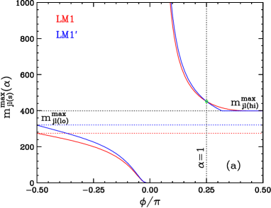
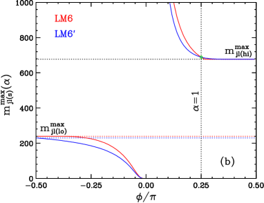
More importantly, many of our new variables from Sec. 2 can provide an independent cross-check on the correct choice for the solution. For example, the kinematic endpoint (35) of the product variable , also violates the symmetry (59) and distinguishes among the two solutions. The infinite set of variables can also be used, and for almost the whole range of . To see this, in Fig. 2 we compare the predictions for the kinematic endpoints of the real and fake solutions, for the two examples discussed in detail in Section 4: (a) the LM1 CMS study point and (b) the LM6 CMS study point. The corresponding mass spectra are listed in Table 1 below. For convenience, we plot versus the parameter
| (60) |
which allows us to map the whole definition domain for into the finite region for . Fig. 2 shows that for most of the allowed range, the two solutions predict different values for the kinematic endpoints . In fact, for , the two predictions are always different, apart from the trivial case of (). Even for , there still exists a range of , for which, at least theoretically, a discrimination can be made. The predictions are guaranteed to coincide only for () (as they should, see (51)), and for a certain range of the largest possible values of .
3.2.2 Invariant mass correlations
Another way to resolve the twofold ambiguity in our solution (57) is to simply go back to the original measurements of and and already at that point try to decide which of the two measured endpoints is and which one is . As already discussed in [18, 46], this identification is in principle possible, if one considers the correlations which are present in the two-dimensional distribution versus . The basic idea is illustrated in Fig. 3, where we show scatter plots of versus , for the two examples used in Fig. 2 and discussed in detail later in Section 4. Fig. 3(a) (Fig. 3(b)) shows the result for the real (fake) solution corresponding to the LM1 study point, while Figs. 3(c) and 3(d) show the analogous results for the LM6 study point. In each plot we used 10,000 entries, which roughly corresponds to () of data for the actual LM1 (LM6) SUSY study point. Here and below we show the ideal case where we neglect smearing effects due to the finite detector resolution, finite particle widths and combinatorial backgrounds. All of our plots are at the parton level (using our own Monte-Carlo phase space generator) and without any cuts. Notice that in order to avoid dealing with the large numerical values of the squared masses, we use a quadratic power scale on both axes, which allows us to preserve the simple shapes of the scatter plots when plotting versus the linear masses themselves.
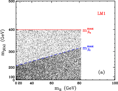
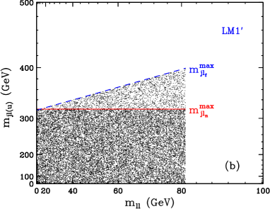
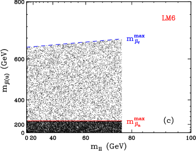
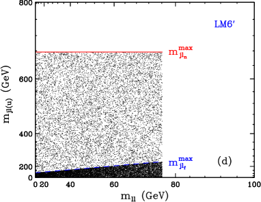
Fig. 3 shows that the combined distribution is simply composed of the two separate distributions and , but they are correlated differently with the dilepton distribution . In particular, let us concentrate on the conditional maxima and , i.e. the maximum allowed values of and , respectively, for a given fixed value of [18, 46]. A close inspection of Fig. 3 shows that the values of and are uncorrelated, and as a result, the conditional maximum does not depend on . In turn, this implies that the endpoint value given in (3) can be obtained for any :
| (61) |
Because of (61), the shape of the versus scatter plot is a simple rectangle [18, 46]. This is confirmed by the plots in Fig. 3, where the (red) horizontal solid line indicates the constant value (61) for the conditional maximum .
In contrast, the values of and are correlated. The conditional maximum does depend on the value of as follows:
| (62) |
where we introduce the shorthand notation used in [47]
| (63) | |||||
| (64) |
The absolute maximum of , which is given by (4) and denoted here by , can only be obtained when itself is at a maximum [18, 46]:
| (65) |
On the other hand, the conditional maximum obtains its minimum value at and corresponds to [18, 46]
| (66) |
Eqs. (65,66) imply that the shape of the versus scatter plot is a right-angle trapezoid. This is confirmed by the plots in Fig. 3, where we mark with a (blue) dashed line the conditional maximum (62). With sufficient statistics, this difference in the kinematic boundaries may be observable, and would reveal the identity of and [18, 46]. Once the individual and are known, the solution for the mass spectrum is unique – see e.g. Appendix A in [47]. Of course, in cases where , namely , it may be difficult in practice to tell which of the two boundaries in the scatter plot is inclined and which one is horizontal888A separate problem, which arises in the case of , will be discussed below in Sec. 4.1.. One example of this sort is offered by point LM6, which has and leads to a rather flat function, as seen in Fig. 3(c).
An alternative and somewhat related method will be to investigate the shapes of the one-dimensional distributions themselves [85]. In Appendix A we provide the analytical expressions for the shapes of the four invariant mass distributions , , and used in our basic analysis from Sec. 3.1. Given what we have already seen in Fig. 3, it is not surprising that the true and the fake solutions predict different shapes for the one-dimensional distributions as well. In the LM1 and LM6 examples considered below in Sec. 4, this difference is particularly noticeable for the and distributions (see Figs. 4(b), 4(d), 5(b) and 5(d)), and can be tested experimentally.
3.2.3 endpoint method
Let us note that if we identify particle with the LSP, we have a rather peculiar situation, in which we know the LSP mass , and we are unsure about the NLSP mass , for which we have to choose among two alternatives. This goes against the common lore which considers the LSP mass (in this case ) to be the least constrained among the masses appearing in the decay chain in Fig. 1. For example, the method of the Cambridge variable [2, 8] treats the LSP mass as a continuous unknown parameter. At this point of our analysis we already know the LSP mass, and we can use this knowledge to our advantage. For example, if we can collect a sufficient number of events of pair-production, we can apply the idea of for the decay as in the original proposal [2]. When we use for the trial LSP mass the known true value of given by (58), the kinematic endpoint of the distribution will reveal the correct value of the mass of the parent particle , thus selecting the true solution in (57).
As emphasized in Ref. [43], the endpoint method does not necessarily rely on being the LSP (i.e. the very last particle in the decay chain) or being the “grandparent” (i.e. the very first particle in the decay chain). For example, suppose that decays further. In that case, one simply needs to apply the more general “subsystem” variable [43] with being the “child” particle: . Similarly, the two particles do not have to be the two grandparents initiating the decay chains: it is sufficient to consider with and arbitrary [43]. Finally, for the purposes of selecting the correct solution in (57) it is also possible to apply the subsystem variable in a different way, where is the child, and the parent is either or . In this case, we know the parent mass, which is respectively given by (53) or (54), and we are asking the question, which of the two test masses in (57) gives the correct answer for the endpoint.
4 Numerical examples
We shall now illustrate the ideas of the previous section with two specific numerical examples: the LM1 and LM6 SUSY study points in CMS [83]. The mass spectra at LM1 and LM6 are listed in Table 1. Point LM1 is similar to benchmark point A (A’) in Ref. [86] (Ref. [87]) and to benchmark point SPS1a in Ref. [88]. Point LM6 is similar to benchmark point C (C’) in Ref. [86] (Ref. [87]). The table also lists the corresponding duplicate solutions LM1’ and LM6’, which are obtained by interchanging , or equivalently, by replacing the mass of via
| (67) |
| Variable | LM1 | LM1’ | LM6 | LM6’ |
|---|---|---|---|---|
| (GeV) | 94.9 | 158.15 | ||
| (GeV) | 118.9 | 143.35 | 291.0 | 165.65 |
| (GeV) | 179.6 | 304.8 | ||
| (GeV) | 561.6 | 861.9 | ||
| 0.6370 | 0.4383 | 0.2954 | 0.9115 | |
| 0.4383 | 0.6370 | 0.9115 | 0.2954 | |
| 0.1023 | 0.1251 | |||
| (GeV) | 81.10 | 76.12 | ||
| (GeV) | 398.8 | 676.8 | ||
| (GeV) | 320.6 | 239.8 | ||
| (GeV) | 451.8 | 689.2 | ||
| (GeV) | 451.8 | 689.2 | ||
| (GeV) | 215.2 | 176.4 | ||
| (GeV) | 398.8 | 676.8 | ||
| (GeV) | 406.6 | 398.8 | 676.8 | 677.0 |
| (GeV) | 417.9 | 402.5 | 676.8 | 678.4 |
| (GeV) | 611.0 | 638.9 | 886.0 | 807.1 |
| (GeV) | 142.9 | 159.7 | 174.9 | 138.0 |
| (GeV) | 200.1 | 225.9 | 224.8 | 184.8 |
| (GeV) | 274.6 | 319.1 | 239.8 | 229.9 |
| (GeV) | 292.0 | 319.4 | 393.7 | 310.9 |
| (GeV) | 398.8 | 320.6 | 239.8 | 676.8 |
| (GeV) | 320.6 | 398.8 | 676.8 | 239.8 |
It is interesting to note that LM1 and LM6 represent both sides of the ambiguity (59): at LM1, we have and correspondingly, and (32) applies. On the other hand, at LM6 we have and , so that (33) applies. Another interesting difference is that at LM1 particle is the right-handed slepton , while at LM6 the role of particle is played999Although the right-handed slepton is also kinematically accessible at point LM6, the wino-like neutralino decays much more often to as opposed to . by the left-handed slepton . Of course, to the extent that we are interested in kinematical features, this difference is not relevant, and particle of the LM6 spectrum may very well have been the right-handed slepton instead.
4.1 Mass measurements at points LM1 and LM6
Given the mass spectra in Table 1, it is straightforward to construct and investigate the relevant invariant mass distributions. For the purposes of illustration, we shall ignore spin correlations, referring the readers interested in those effects to Refs. [52, 58, 71]. We are justified to do so for several reasons. First, our method relies on the measurement of kinematic endpoints, whose location is unaffected by the presence of spin correlations. Second, in the case of supersymmetry (which is really what we have in mind here), particle is a scalar, which automatically washes out any spin effects in the and distributions. Furthermore, if particles and their antiparticles are produced in equal numbers, as would be the case if the dominant production is from and/or initial state, any spin correlations in the distribution are also washed out. Under those circumstances, therefore, the pure phase space distributions shown here are in fact the correct answer.
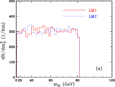
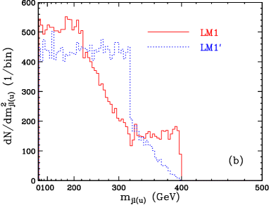
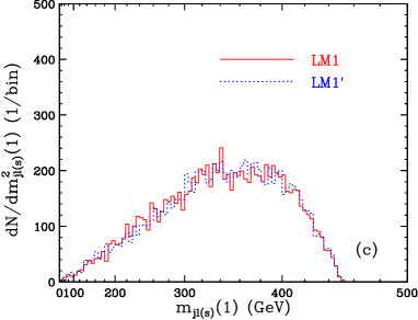
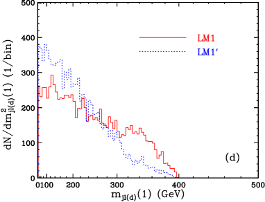
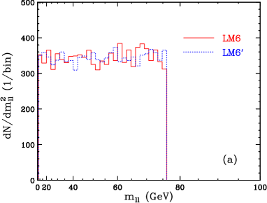
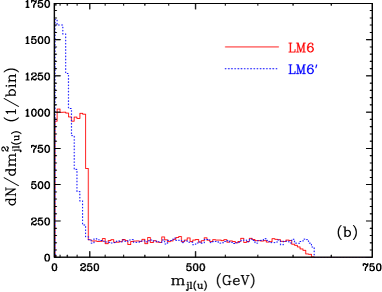
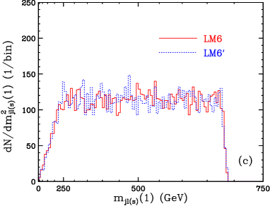
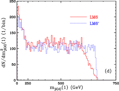
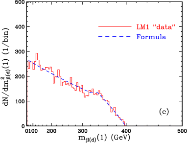
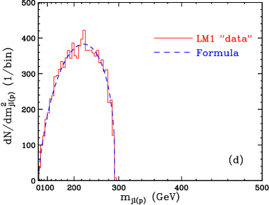
We begin our discussion with the four invariant mass distributions , , and , which form the basis of our method outlined in Sec. 3.1. Fig. 4 (Fig. 5) shows those four distributions for the case of study point LM1 (LM6). In each panel, the red (solid) histogram corresponds to the nominal spectrum (LM1 or LM6), while the blue (dotted) histogram corresponds to the “fake” solution (LM1’ or LM6’), which is obtained through the replacement (67). For all figures in this section, we use the same 4 samples of 10,000 events each, which were already used to make Fig. 3. Notice our somewhat unconventional way of filling and then plotting the histograms in this section. First, we show differential distributions in the corresponding mass squared, i.e. . This is done in order to preserve the connection to the analytical results in Appendix A, which are written the same way. More importantly, the shapes of the one-dimensional histograms are much simpler in the case of as opposed to [52, 58, 71]. In the next step, however, we choose to plot the thus obtained histogram versus the mass itself rather than the mass squared. This allows one to read off immediately the corresponding endpoint and compare directly to the values listed in Table 1. It also keeps the -axis range within a manageable range. However, since the histograms were binned on a mass squared scale, if we were to use a linear scale on the -axis, we would get bins with varying size. This would be rather inconvenient and more importantly, would distort the nice simple shapes of the distributions. Therefore, we use a quadratic scale on the -axis, which preserves the nice shapes and leads to a constant bin size on each plot.
Figs. 4 and 5 illustrate how each one of the measurements (51) can be obtained. For example, is the classic upper kinematic endpoint of the distributions in Figs. 4(a) and 5(a). This endpoint is very sharp and should be easily observable. is the absolute upper kinematic endpoint seen in the combined distribution in Figs. 4(b) and 5(b). Notice that the same endpoint can independently also be observed as the absolute upper kinematic limit of the difference distributions shown in Figs. 4(d) and 5(d). The fact that there are two independent ways of getting to the endpoint should allow for a reasonable accuracy of its measurement. Upon closer inspection of the combined distribution in Figs. 4(b) and 5(b), we also notice the intermediate kinematic endpoint seen around 320 GeV in Fig. 4(b) and around 240 GeV in Fig. 5(b). Finally, is the upper kinematic endpoint of the distribution shown in Figs. 4(c) and 5(c). It is also rather well defined, and should be well measured in the real data.
At this point we would like to comment on one potential problem which is not immediately obvious, but nevertheless has been encountered in practical applications of the invariant mass technique for SUSY mass determinations [85]. It has been noted that in the case of (see eqs. (63,64)), the numerical fit for the mass spectrum becomes rather unstable. Given our analytical results in Sec. 3.1, we are now able to trace the root of the problem. Notice that implies that . In this limit, from eqs. (2), (3), (4) and (44) we find
| (68) |
This means that the functions (53-58) giving the solution for the mass spectrum will all behave as , and, given the statistical fluctuations in an actual analysis, will have very poor convergence properties. We note that this problem is not limited to our preferred set of measurements (51) and is rather generic, but has been missed in most previous studies simply because the case of was rarely considered.
Figs. 4 and 5 reveal that, as expected, the real (red solid lines) and fake (blue dotted lines) solutions always give identical results for our basic set of four endpoint measurements (51). This is by design, and in order to discriminate among the real and the fake solution, we need additional experimental input, as discussed in Section 3.2. Before we proceed with the disambiguation analysis in the next subsection, we should stress once again that the real and fake solutions agree on 75% of the relevant mass spectrum, i.e. they give the same values for the masses of particles , and (see Table 1). The only question mark at this point is, what is the mass of particle . This issue is addressed in the following subsection.
4.2 Eliminating the fake solution for
As already discussed in Section 3.2, there are several handles which could discriminate among the two alternative values of in the real and the fake solution. One possibility, reviewed in Sec. 3.2.3, is to use additional independent measurements of kinematic endpoints. We shall not pursue this direction here, referring the interested readers to Ref. [43] for details. Another possibility, discussed in Sec. 3.2.2 and demonstrated explicitly with Fig. 3, is to use the different correlations in the 2-dimensional invariant mass distributions and . The near-far lepton ambiguity is avoided by studying the scatter plot of , shown in Fig. 3, which should be in principle sufficient to discriminate among the two alternatives.
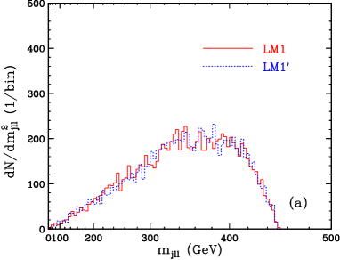
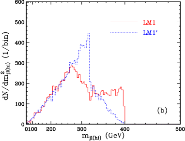
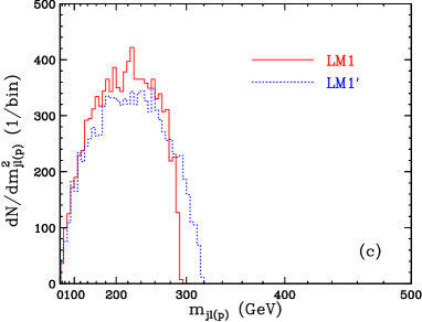
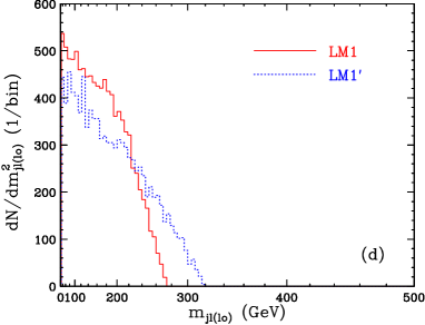
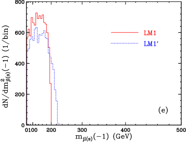
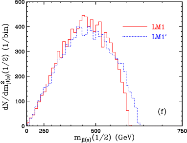
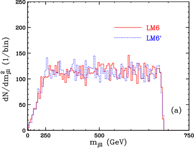
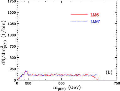
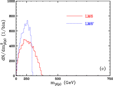
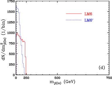
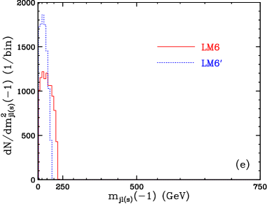
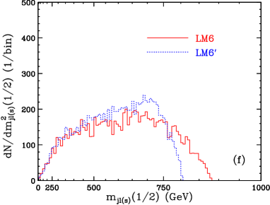
In keeping with the main theme of this paper, in this subsection we shall concentrate on the third possibility, already suggested in Sec. 3.2.1. We shall simply explore additional invariant mass endpoint measurements, which would hopefully discriminate among the two solutions for . Figs. 6 and 7 show several invariant mass distributions which have already been mentioned at one point or another in the course of our previous discussion. Fig. 6 shows the following 6 distributions: (a) ; (b) ; (c) ; (d) ; (e) and (f) , for the LM1 mass spectrum (red solid lines) and its LM1’ counterpart (blue dotted lines). Fig. 7 shows the same 6 distributions, but for the LM6 and LM6’ mass spectra. In both figures, we follow the same plotting conventions as in Figs. 4 and 5: we form the mass squared distribution , and then plot versus the corresponding linear mass using a quadratic scale on the -axis. Notice that the sum of the distribution in Fig. 6(b) (Fig. 7(b)) and the distribution in Fig. 6(d) (Fig. 7(d)) precisely equals the combined distribution in Fig. 4(b) (Fig. 5(b)). In order to be able to see this by the naked eye, we have kept the same and ranges on the corresponding plots.
As seen in Figs. 6 and 7, not all of the remaining invariant mass distributions are able to discriminate among the two solutions. As explained in Sec. 3.2.1, the suitable distributions are those whose endpoints violate the symmetry (59), which caused the ambiguity in the first place. For example, Figs. 6(a) and 7(a) show that the endpoint of the distribution is the same for the real and the fake solution. This is to be expected, since the defining expression (9) for is symmetric under (59). Figs. 6(a) and 7(a) also show that even the shapes of the distributions for the real and fake solution are very similar. In spite of this, the observation of the endpoint can still be very useful, e.g. in reducing the experimental error on the mass determination.
Similar comments apply to the distributions shown in Figs. 6(b) and 7(b). Here again the endpoint is a symmetric function of and , and the real and fake solutions predict identical endpoints. However, while the endpoints are the same, this time the shapes are not. The shape difference is more pronounced in the case of LM1 shown in Fig. 6(b), and less visible in the case of LM6 shown in Fig. 7(b).
The remaining four distributions shown in Figs. 6(c-f) and 7(c-f) already have different endpoints and can thus be used for discrimination among the real and fake solution for . All of the endpoints in Figs. 6(c-f) and 7(c-f) are relatively sharp and should be measured rather well. One should not forget that in Figs. 6 and 7 we show distributions for only three representative values of : in panels (d), in panels (e), and in panels (f). As seen in Fig. 2, there are infinitely many other choices for , which would still exhibit different endpoints for the real and fake solutions. Our conclusion is that through a suitable combination of additional endpoint measurements one would be able to tell apart the real solution for from its fake cousin.
5 Summary and conclusions
In this paper we revisited the classic technique for SUSY mass determinations via invariant mass endpoints. We set out to redesign the standard algorithm for performing these studies, by pursuing two main objectives (see Section 1.4):
-
•
Improving on the experimental precision of the SUSY mass determination. For example, we required that our analysis be based exclusively on upper invariant mass endpoints, which are expected to be measured with a greater precision than the corresponding lower endpoints (a.k.a. thresholds). Consequently, we did not make use of the “threshold” measurement , which has been an integral part of most SUSY studies since Ref. [7]. In the same vein, we also demanded that we should not rely on any features observed in a two- or a three-dimensional invariant mass distribution — such measurements are expected to be less precise than the (upper) endpoints extracted from simple one-dimensional histograms.
-
•
Avoiding any parameter space region ambiguities. It is well known that some of the invariant mass endpoints used in the conventional analyses are piecewise-defined functions. This feature may sometimes lead to multiple solutions for the SUSY mass spectrum in the “LHC inverse problem” [12, 78, 79, 80, 47]. In order to safeguard against this possibility, we conservatively demanded from the outset that none of our endpoint measurements be given by piecewise defined functions. This rather strict requirement rules out three of the standard endpoint measurements , , and .
In order to meet these objectives, in Section 2 we proposed a set of new invariant mass variables whose upper kinematic endpoints can be alternatively used for SUSY mass reconstruction studies. Then in Section 3 we outlined a simple analysis which was based on the particular set of four invariant mass variables (51), all of which satisfy our requirements. In Section 3.1 we provided simple analytical formulas for the SUSY mass spectrum in terms of the four measured endpoints in eq. (51). Our solutions revealed a surprise: in spite of the two-fold ambiguity (32,33) in the interpretation of two of our endpoints and , the answer for three (, and ) out of the four SUSY masses is unique! The fourth mass () is also known, up to the two-fold ambiguity (67), which can be easily resolved by a variety of methods discussed and illustrated in Sections 3.2 and 4.2. In Section 4 we applied our technique to two specific examples — the LM1 and LM6 CMS study points.
Our method contains a number of elements which help in achieving our two main objectives. For example, the precision of the SUSY mass determination is expected to improve, due to the following factors:
-
1.
Precise knowledge of the whole shape of the invariant mass distribution. In Appendix A we list the analytical expressions for all differential invariant mass distributions used in our basic analysis from Section 3.1: , and . We also provide the corresponding expression for the distribution, whose upper endpoint offers an independent measurement of (see eq. (49)). Finally, we also list the formula for the differential distribution of , whose endpoint can be used for selecting the correct solution, as shown in Figs. 6(c) and 7(c). The knowledge of the shape of the whole distribution is indispensable and greatly improves the accuracy of the endpoint extraction. In the absence of any analytical results like those in Appendix A, one would be forced to use simple linear extrapolations, which would lead to a significant systematic error.
-
2.
The number of available measurements tremendously exceeds the number of unknown mass parameters. In principle, in order to extract 4 mass parameters, one needs a set of 4 measurements, for which we chose (51). On the other hand, Section 2 contains a number of additional variables, whose endpoints will also be measured, and possibly even better than our basic set (51). The addition of these extra measurements cannot hurt, and can only improve the overall accuracy of the SUSY mass determinations.
-
3.
Improved precision on the endpoint measurements. Clearly, not all invariant mass variables will have their endpoints measured with exactly the same precision – some endpoints will be measured better than others. This difference can be due to many factors, e.g. the slope of the distribution near the endpoint, the shape (convex versus concave) of the distribution near the endpoint, the actual location of the endpoint, the level of SM and SUSY combinatorial background near the endpoint, etc. Our analysis in Sec. 3.1 was based on a specific set of 4 endpoint measurements (51), which were chosen due to the simplicity in their theoretical interpretation. However, these may not necessarily be the best measured endpoints. In fact one can already anticipate from Figs. 6 and 7 that the endpoints of some of the , , and distributions might be measured even better. For example, the distributions in Figs. 6(c), 6(e) and 6(f) are all steeper near their endpoints, compared to the distribution in Fig. 4(c) that we used. By the same token, one might expect that the endpoints in Figs. 7(a), 7(d) and 7(e) will be measured more precisely than the upper endpoints of Figs. 5(b) and 5(d).
-
4.
Controlled selection of an optimum set of measurements. Notice that the variable defined in eq. (36) depends on a continuous parameter whose value can be dialed up by the experimenter at will. This has several advantages. For example, as we have seen in Fig. 2, the discriminating power of in rejecting the wrong solution in (57) depends on the value of . Having obtained a preliminary information about the two competing solutions, one can then choose the optimum value (or a range of values) for for a subsequent study. Similarly, after the initial solution for the mass spectrum has been obtained, one can analyze by Monte Carlo the shapes of the distributions as a function of and select for further study specific values of for which the corresponding endpoints are expected to be measured with a much better experimental precision.
In meeting our second objective, our method shows a certain improvement on the theoretical side as well:
-
1.
Reduced sensitivity to the parameter space region. All of the new variables introduced in Sec. 2 exhibit milder sensitivity to the parameter space region, in comparison to the conventional endpoint . As can be seen from the formulas in Sec. 2, the endpoint for each of our variables is given by at most two different expressions, as opposed to four in the case of . A notable exception is the variable , whose endpoint is actually uniquely predicted, and is independent of the parameter space region. We therefore strongly encourage the use of in future analyses of SUSY mass determinations.
-
2.
Uniqueness of the solution. It is worth emphasizing that with only the 4 measurements of eq. (51) we can already uniquely determine three out of the four masses involved in the problem. Then, the addition of a fifth measurement, as discussed in Secs. 3.2.1 and 4.2, is sufficient to pin down all four of the SUSY masses. In contrast, with the conventional approach, one also starts with four measurements as in (22), but in the worst case scenario this results in infinitely many solutions, due to the linear dependence problem (24) discussed in Section 1.2. Adding a fifth measurement as in (28) helps, but once again, the worst case scenario leads to two alternative solutions [47]. In order to resolve the remaining duplication, and thus guarantee uniqueness of the solution under any circumstances, one needs at least 6 measurements.
In conclusion, our main accomplishment in this paper was to expand the experimenter’s arsenal with several new tools which can be used for SUSY mass determinations via kinematic endpoints. We believe that the variables suggested in Section 2 and the shapes of their distributions listed in Appendix A will eventually find their way into the actual experimental analyses after the discovery of SUSY (or any other new physics exhibiting the decay chain of Fig. 1).
Acknowledgments.
We thank M. Burns for collaboration in the early stages of this project. This work is supported in part by a US Department of Energy grant DE-FG02-97ER41029.Appendix A Appendix: Analytical expressions for the shapes of the invariant mass distributions
In this appendix we will provide the analytical expressions for the shapes of the invariant mass distributions , , , , and . To simplify the expressions, we introduce the shorthand notation for the corresponding endpoints, which was already introduced in (52), (61), (63) and (64):
| (A.1) | |||||
| (A.2) | |||||
| (A.3) | |||||
| (A.4) |
In this appendix, we shall ignore spin correlations and consider only pure phase space decays. General results including spin correlations for , and exist and can be found in [71]. We shall unit-normalize the , , and distributions, to which each event contributes a single entry. In contrast, the union distribution has two entries per event, so it will be normalized to 2 instead. It is also convenient to write the distributions in terms of masses squared instead of linear masses. Of course, the two are trivially related by
| (A.5) |
A.1 Dilepton mass distribution
The differential dilepton invariant mass distribution is given by
| (A.6) |
which is unit-normalized:
| (A.7) |
A.2 Combined jet-lepton mass distribution
The differential distribution for is given by
| (A.8) |
where is the usual Heaviside step function
| (A.9) |
It is easy to verify the normalization condition
| (A.10) |
where was already defined in (52).
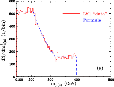
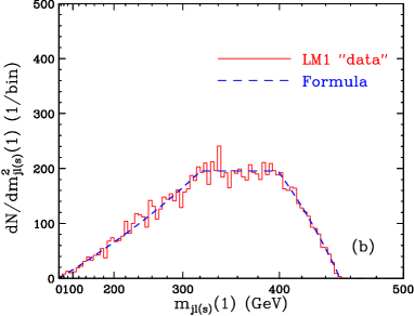
A.3 Distribution of the sum
A.4 Distribution of the difference
The differential distribution for the difference depends on the values of and . To simplify the notation, we define an antisymmetric function
| (A.13) |
which we heavily use in writing down the result for the differential distribution. Notice that there are various equivalent ways to write down these formulas, due to the transitivity property
| (A.14) |
For one needs to consider
five separate cases:
If , then
| (A.15) | |||||
If , then
| (A.16) | |||||
If , then
| (A.17) | |||||
If , then
| (A.18) | |||||
If , then
| (A.19) | |||||
The normalization condition now reads
| (A.20) |
A.5 Distribution of the product
Finally, for completeness we also list the differential distribution for the product variable (34), for which here we shall use the shorthand notation . To further simplify the notation, we define the function
| (A.21) |
where , and are defined as before in (A.2-A.4).
There are two separate cases:
If , the distribution is made up of two branches joining at (see, for example the LM1 distribution in Fig. 6(c) and the LM6’ distribution in Fig. 7(c))
| (A.22) | |||||
If , there is a single branch, as illustrated by the LM1’ distribution in Fig. 6(c) and the LM6 distribution in Fig. 7(c):
| (A.23) |
In both of those cases, the normalization condition is
| (A.24) |
where is the corresponding endpoint defined in (35).
References
- [1] I. Hinchliffe, F. E. Paige, M. D. Shapiro, J. Soderqvist and W. Yao, “Precision SUSY measurements at LHC,” Phys. Rev. D 55, 5520 (1997) [arXiv:hep-ph/9610544].
- [2] C. G. Lester and D. J. Summers, “Measuring masses of semi-invisibly decaying particles pair produced at hadron colliders,” Phys. Lett. B 463, 99 (1999) [arXiv:hep-ph/9906349].
- [3] H. Bachacou, I. Hinchliffe and F. E. Paige, “Measurements of masses in SUGRA models at LHC,” Phys. Rev. D 62, 015009 (2000) [arXiv:hep-ph/9907518].
- [4] I. Hinchliffe and F. E. Paige, “Measurements in SUGRA models with large tan(beta) at LHC,” Phys. Rev. D 61, 095011 (2000) [arXiv:hep-ph/9907519].
- [5] ATLAS collaboration, ATLAS detector and physics performance, ATLAS TDR 15, CERN/LHCC 99-15
- [6] M. M. Nojiri, D. Toya and T. Kobayashi, “Lepton Energy Asymmetry and Precision SUSY study at Hadron Colliders,” Phys. Rev. D 62, 075009 (2000) [arXiv:hep-ph/0001267].
- [7] B. C. Allanach, C. G. Lester, M. A. Parker and B. R. Webber, “Measuring sparticle masses in non-universal string inspired models at the LHC,” JHEP 0009, 004 (2000) [arXiv:hep-ph/0007009].
- [8] A. Barr, C. Lester and P. Stephens, “m(T2): The truth behind the glamour,” J. Phys. G 29, 2343 (2003) [arXiv:hep-ph/0304226].
- [9] M. M. Nojiri, G. Polesello and D. R. Tovey, “Proposal for a new reconstruction technique for SUSY processes at the LHC,” arXiv:hep-ph/0312317.
- [10] Christopher Gorham Lester, Model independent sparticle mass measurements at ATLAS, A dissertation submitted to the University of Cambridge for the degree of Doctor of Philosophy December 2001.
- [11] K. Kawagoe, M. M. Nojiri and G. Polesello, “A new SUSY mass reconstruction method at the CERN LHC,” Phys. Rev. D 71, 035008 (2005) [arXiv:hep-ph/0410160].
- [12] B. K. Gjelsten, D. J. Miller and P. Osland, “Measurement of SUSY masses via cascade decays for SPS 1a,” JHEP 0412, 003 (2004) [arXiv:hep-ph/0410303].
- [13] B. K. Gjelsten, D. J. Miller and P. Osland, “Measurement of the gluino mass via cascade decays for SPS 1a,” JHEP 0506, 015 (2005) [arXiv:hep-ph/0501033].
- [14] A. Birkedal, R. C. Group and K. Matchev, “Slepton mass measurements at the LHC,” In the Proceedings of 2005 International Linear Collider Workshop (LCWS 2005), Stanford, California, 18-22 Mar 2005, pp 0210 [arXiv:hep-ph/0507002].
- [15] C. G. Lester, M. A. Parker and M. J. . White, “Determining SUSY model parameters and masses at the LHC using cross-sections, kinematic edges and other observables,” JHEP 0601, 080 (2006) [arXiv:hep-ph/0508143].
- [16] D. J. Miller, P. Osland and A. R. Raklev, “Invariant mass distributions in cascade decays,” JHEP 0603, 034 (2006) [arXiv:hep-ph/0510356].
- [17] P. Meade and M. Reece, “Top partners at the LHC: Spin and mass measurement,” Phys. Rev. D 74, 015010 (2006) [arXiv:hep-ph/0601124].
- [18] Luc Pape, “Reconstruction of sparticle masses from endpoints (and others) at LHC”, CMS Internal Note CMS IN-2006/12.
- [19] C. G. Lester, “Constrained invariant mass distributions in cascade decays: The shape of the ’m(qll)-threshold’ and similar distributions,” Phys. Lett. B 655, 39 (2007) [arXiv:hep-ph/0603171].
- [20] C. G. Lester, M. A. Parker and M. J. . White, “Three body kinematic endpoints in SUSY models with non-universal Higgs masses,” JHEP 0710 (2007) 051 [arXiv:hep-ph/0609298].
- [21] B. K. Gjelsten, D. J. Miller, P. Osland and A. R. Raklev, “Mass determination in cascade decays using shape formulas,” AIP Conf. Proc. 903, 257 (2007) [arXiv:hep-ph/0611259].
- [22] S. Matsumoto, M. M. Nojiri and D. Nomura, “Hunting for the top partner in the littlest Higgs model with T-parity at the LHC,” Phys. Rev. D 75, 055006 (2007) [arXiv:hep-ph/0612249].
- [23] H. C. Cheng, J. F. Gunion, Z. Han, G. Marandella and B. McElrath, “Mass Determination in SUSY-like Events with Missing Energy,” JHEP 0712, 076 (2007) [arXiv:0707.0030 [hep-ph]].
- [24] C. Lester and A. Barr, “MTGEN : Mass scale measurements in pair-production at colliders,” JHEP 0712, 102 (2007) [arXiv:0708.1028 [hep-ph]].
- [25] W. S. Cho, K. Choi, Y. G. Kim and C. B. Park, “Gluino Stransverse Mass,” Phys. Rev. Lett. 100, 171801 (2008) [arXiv:0709.0288 [hep-ph]].
- [26] B. Gripaios, “Transverse Observables and Mass Determination at Hadron Colliders,” JHEP 0802, 053 (2008) [arXiv:0709.2740 [hep-ph]].
- [27] A. J. Barr, B. Gripaios and C. G. Lester, “Weighing Wimps with Kinks at Colliders: Invisible Particle Mass Measurements from Endpoints,” JHEP 0802, 014 (2008) [arXiv:0711.4008 [hep-ph]].
- [28] W. S. Cho, K. Choi, Y. G. Kim and C. B. Park, “Measuring superparticle masses at hadron collider using the transverse mass kink,” JHEP 0802, 035 (2008) [arXiv:0711.4526 [hep-ph]].
- [29] G. G. Ross and M. Serna, “Mass Determination of New States at Hadron Colliders,” Phys. Lett. B 665, 212 (2008) [arXiv:0712.0943 [hep-ph]].
- [30] M. M. Nojiri, G. Polesello and D. R. Tovey, “A hybrid method for determining SUSY particle masses at the LHC with fully identified cascade decays,” JHEP 0805, 014 (2008) [arXiv:0712.2718 [hep-ph]].
- [31] P. Huang, N. Kersting and H. H. Yang, “Hidden Thresholds: A Technique for Reconstructing New Physics Masses at Hadron Colliders,” arXiv:0802.0022 [hep-ph].
- [32] M. M. Nojiri, Y. Shimizu, S. Okada and K. Kawagoe, “Inclusive transverse mass analysis for squark and gluino mass determination,” JHEP 0806, 035 (2008) [arXiv:0802.2412 [hep-ph]].
- [33] D. R. Tovey, “On measuring the masses of pair-produced semi-invisibly decaying particles at hadron colliders,” JHEP 0804, 034 (2008) [arXiv:0802.2879 [hep-ph]].
- [34] M. M. Nojiri and M. Takeuchi, “Study of the top reconstruction in top-partner events at the LHC,” arXiv:0802.4142 [hep-ph].
- [35] H. C. Cheng, D. Engelhardt, J. F. Gunion, Z. Han and B. McElrath, “Accurate Mass Determinations in Decay Chains with Missing Energy,” Phys. Rev. Lett. 100, 252001 (2008) [arXiv:0802.4290 [hep-ph]].
- [36] W. S. Cho, K. Choi, Y. G. Kim and C. B. Park, “Measuring the top quark mass with at the LHC,” Phys. Rev. D 78, 034019 (2008) [arXiv:0804.2185 [hep-ph]].
- [37] M. Serna, “A short comparison between and ,” JHEP 0806, 004 (2008) [arXiv:0804.3344 [hep-ph]].
- [38] M. Bisset, R. Lu and N. Kersting, “Improving SUSY Spectrum Determinations at the LHC with Wedgebox and Hidden Threshold Techniques,” arXiv:0806.2492 [hep-ph].
- [39] A. J. Barr, G. G. Ross and M. Serna, “The Precision Determination of Invisible-Particle Masses at the LHC,” arXiv:0806.3224 [hep-ph].
- [40] N. Kersting, “On Measuring Split-SUSY Gaugino Masses at the LHC,” arXiv:0806.4238 [hep-ph].
- [41] M. M. Nojiri, K. Sakurai, Y. Shimizu and M. Takeuchi, “Handling jets + missing channel using inclusive mT2,” arXiv:0808.1094 [hep-ph].
- [42] H. C. Cheng and Z. Han, “Minimal Kinematic Constraints and ,” JHEP 0812, 063 (2008) [arXiv:0810.5178 [hep-ph]].
- [43] M. Burns, K. Kong, K. T. Matchev and M. Park, “Using Subsystem for Complete Mass Determinations in Decay Chains with Missing Energy at Hadron Colliders,” JHEP 0903, 143 (2009) arXiv:0810.5576 [hep-ph].
- [44] A. J. Barr, A. Pinder and M. Serna, “Precision Determination of Invisible-Particle Masses at the CERN LHC: II,” arXiv:0811.2138 [hep-ph].
- [45] P. Konar, K. Kong and K. T. Matchev, “: a global inclusive variable for determining the mass scale of new physics in events with missing energy at hadron colliders,” JHEP 0903, 085 (2009) [arXiv:0812.1042 [hep-ph]].
- [46] D. Costanzo and D. R. Tovey, “Supersymmetric particle mass measurement with invariant mass correlations,” JHEP 0904, 084 (2009) [arXiv:0902.2331 [hep-ph]].
- [47] M. Burns, K. T. Matchev and M. Park, “Using kinematic boundary lines for particle mass measurements and disambiguation in SUSY-like events with missing energy,” JHEP 0905, 094 (2009) arXiv:0903.4371 [hep-ph].
- [48] J. Alwall, K. Hiramatsu, M. M. Nojiri and Y. Shimizu, “Novel reconstruction technique for New Physics processes with initial state radiation,” arXiv:0905.1201 [hep-ph].
- [49] H. C. Cheng, J. F. Gunion, Z. Han and B. McElrath, “Accurate Mass Determinations in Decay Chains with Missing Energy: II,” arXiv:0905.1344 [hep-ph].
- [50] A. J. Barr, “Using lepton charge asymmetry to investigate the spin of supersymmetric particles at the LHC,” Phys. Lett. B 596, 205 (2004) [arXiv:hep-ph/0405052].
- [51] M. Battaglia, A. Datta, A. De Roeck, K. Kong and K. T. Matchev, “Contrasting supersymmetry and universal extra dimensions at the CLIC multi-TeV e+ e- collider,” JHEP 0507, 033 (2005) [arXiv:hep-ph/0502041].
- [52] J. M. Smillie and B. R. Webber, “Distinguishing spins in supersymmetric and universal extra dimension models at the Large Hadron Collider,” JHEP 0510, 069 (2005) [arXiv:hep-ph/0507170].
- [53] M. Battaglia, A. K. Datta, A. De Roeck, K. Kong and K. T. Matchev, “Contrasting supersymmetry and universal extra dimensions at colliders,” In the Proceedings of 2005 International Linear Collider Workshop (LCWS 2005), Stanford, California, 18-22 Mar 2005, pp 0302 [arXiv:hep-ph/0507284].
- [54] A. Datta, K. Kong and K. T. Matchev, “Discrimination of supersymmetry and universal extra dimensions at hadron colliders,” Phys. Rev. D 72, 096006 (2005) [Erratum-ibid. D 72, 119901 (2005)] [arXiv:hep-ph/0509246].
- [55] A. Datta, G. L. Kane and M. Toharia, “Is it SUSY?,” arXiv:hep-ph/0510204.
- [56] A. J. Barr, “Measuring slepton spin at the LHC,” JHEP 0602, 042 (2006) [arXiv:hep-ph/0511115].
- [57] A. Alves, O. Eboli and T. Plehn, “It’s a gluino,” Phys. Rev. D 74, 095010 (2006) [arXiv:hep-ph/0605067].
- [58] C. Athanasiou, C. G. Lester, J. M. Smillie and B. R. Webber, “Distinguishing spins in decay chains at the Large Hadron Collider,” JHEP 0608, 055 (2006) [arXiv:hep-ph/0605286].
- [59] L. T. Wang and I. Yavin, “Spin Measurements in Cascade Decays at the LHC,” JHEP 0704, 032 (2007) [arXiv:hep-ph/0605296].
- [60] C. Athanasiou, C. G. Lester, J. M. Smillie and B. R. Webber, “Addendum to ’Distinguishing spins in decay chains at the Large Hadron Collider’,” arXiv:hep-ph/0606212.
- [61] S. Abdullin et al. [TeV4LHC Working Group], “Tevatron-for-LHC report: Preparations for discoveries,” arXiv:hep-ph/0608322.
- [62] J. M. Smillie, “Spin Correlations in Decay Chains Involving W Bosons,” Eur. Phys. J. C 51, 933 (2007) [arXiv:hep-ph/0609296].
- [63] K. Kong and K. T. Matchev, “Phenomenology of universal extra dimensions,” AIP Conf. Proc. 903, 451 (2007) [arXiv:hep-ph/0610057].
- [64] C. Kilic, L. T. Wang and I. Yavin, “On the Existence of Angular Correlations in Decays with Heavy Matter Partners,” JHEP 0705, 052 (2007) [arXiv:hep-ph/0703085].
- [65] A. Alves and O. Eboli, “Unravelling the sbottom spin at the CERN LHC,” Phys. Rev. D 75, 115013 (2007) [arXiv:0704.0254 [hep-ph]].
- [66] C. Csaki, J. Heinonen and M. Perelstein, “Testing Gluino Spin with Three-Body Decays,” JHEP 0710, 107 (2007) [arXiv:0707.0014 [hep-ph]].
- [67] A. Datta, P. Dey, S. K. Gupta, B. Mukhopadhyaya and A. Nyffeler, “Distinguishing the Littlest Higgs model with T-parity from supersymmetry at the LHC using trileptons,” Phys. Lett. B 659, 308 (2008) [arXiv:0708.1912 [hep-ph]].
- [68] M. R. Buckley, H. Murayama, W. Klemm and V. Rentala, “Discriminating spin through quantum interference,” arXiv:0711.0364 [hep-ph].
- [69] M. R. Buckley, B. Heinemann, W. Klemm and H. Murayama, “Quantum Interference Effects Among Helicities at LEP-II and Tevatron,” Phys. Rev. D 77, 113017 (2008) [arXiv:0804.0476 [hep-ph]].
- [70] G. L. Kane, A. A. Petrov, J. Shao and L. T. Wang, “Initial determination of the spins of the gluino and squarks at LHC,” arXiv:0805.1397 [hep-ph].
- [71] M. Burns, K. Kong, K. T. Matchev and M. Park, “A General Method for Model-Independent Measurements of Particle Spins, Couplings and Mixing Angles in Cascade Decays with Missing Energy at Hadron Colliders,” JHEP 0810, 081 (2008), arXiv:0808.2472 [hep-ph].
- [72] W. S. Cho, K. Choi, Y. G. Kim and C. B. Park, “-assisted on-shell reconstruction of missing momenta and its application to spin measurement at the LHC,” Phys. Rev. D 79, 031701 (2009) arXiv:0810.4853 [hep-ph].
- [73] M. Graesser and J. Shelton, “Probing Supersymmetry With Third-Generation Cascade Decays,” arXiv:0811.4445 [hep-ph].
- [74] G. Hallenbeck, M. Perelstein, C. Spethmann, J. Thom and J. Vaughan, “Model Discrimination with the CMS Detector: a Case Study,” arXiv:0812.3135 [hep-ph].
- [75] O. Gedalia, S. J. Lee and G. Perez, “Spin Determination via Third Generation Cascade Decays,” arXiv:0901.4438 [hep-ph].
- [76] F. Boudjema and R. K. Singh, “A model independent spin analysis of fundamental particles using azimuthal asymmetries,” arXiv:0903.4705 [hep-ph].
- [77] H. C. Cheng, K. T. Matchev and M. Schmaltz, “Bosonic supersymmetry? Getting fooled at the CERN LHC,” Phys. Rev. D 66, 056006 (2002) [arXiv:hep-ph/0205314].
- [78] N. Arkani-Hamed, G. L. Kane, J. Thaler and L. T. Wang, “Supersymmetry and the LHC inverse problem,” JHEP 0608, 070 (2006) [arXiv:hep-ph/0512190].
- [79] B. K. Gjelsten, D. J. Miller and P. Osland, “Resolving ambiguities in mass determinations at future colliders,” In the Proceedings of 2005 International Linear Collider Workshop (LCWS 2005), Stanford, California, 18-22 Mar 2005, pp 0211 [arXiv:hep-ph/0507232].
- [80] B. K. Gjelsten, D. J. Miller, P. Osland and A. R. Raklev, “Mass ambiguities in cascade decays,” arXiv:hep-ph/0611080.
- [81] M. Park, Ambiguities in SUSY mass determination from kinematic endpoints at LHC, talk given at the Pheno 2008 Symposium “LHC Turn On”, Madison WI, April 28, 2008.
- [82] K. Matchev, New Physics Signatures and Precision Measurements at the LHC, talk given at the KITP Conference: “Anticipating Physics at the LHC Collider”, UC Santa Barbara, June 5, 2008.
- [83] G. L. Bayatian et al. [CMS Collaboration], “CMS technical design report, volume II: Physics performance,” J. Phys. G 34, 995 (2007).
- [84] F. Heinemann, “The discovery potential of the in mSUGRA in the -channel at high at the LHC”, Diploma thesis, ETH Zurich, Switzerland, March 2004.
- [85] Georgia Karapostoli, “Observation and measurement of the supersymmetric process with the CMS experiment at LHC”, CMS thesis CMS TS-2009/007.
- [86] M. Battaglia et al., “Proposed post-LEP benchmarks for supersymmetry,” Eur. Phys. J. C 22, 535 (2001) [arXiv:hep-ph/0106204].
- [87] M. Battaglia, A. De Roeck, J. R. Ellis, F. Gianotti, K. A. Olive and L. Pape, “Updated post-WMAP benchmarks for supersymmetry,” Eur. Phys. J. C 33, 273 (2004) [arXiv:hep-ph/0306219].
- [88] B. C. Allanach et al., “The Snowmass points and slopes: Benchmarks for SUSY searches,” in Proc. of the APS/DPF/DPB Summer Study on the Future of Particle Physics (Snowmass 2001) ed. N. Graf, Eur. Phys. J. C 25, 113 (2002) [arXiv:hep-ph/0202233].