The Acoustic Peak in the Lyman Alpha Forest

Abstract

We present the first simulation of the signature of baryonic acoustic oscillations (BAO) in Lyman-$\alpha$ forest data containing 180,000 mock quasar sight-lines. We use eight large dark-matter only simulations onto which we paint the Lyman-$\alpha$ field using the fluctuating Gunn-Peterson approximation. We argue that this approach should be sufficient for the mean signature on the scales of interest. Our results indicate that Lyman-$\alpha$ flux provides a good tracer of the underlying dark matter field on large scales and that redshift space distortions are well described by a simple linear theory prescription. We compare Fourier and configuration space approaches to describing the signal and argue that configuration space statistics provide useful data compression. We also investigate the effect of a fluctuating photo-ionizing background using a simplified model and find that such fluctuations do add smooth power on large scales. The acoustic peak position is, however, unaffected for small amplitude fluctuations ($<10\%$). Larger amplitude fluctuations make the recovery of the BAO signal more difficult and may degrade the achievable significance of the measurement.

I Introduction

Oscillations of the baryon-photon plasma in the early universe, also known as Baryon Acoustic Oscillations (BAO), imprint a distinct signature on the clustering of matter (Peebles and Yu, 1970; Sunyaev and Zeldovich, 1970). The distance that acoustic waves propagate in the first several hundred thousand years of cosmic evolution set a characteristic scale that is measurable as a distinct peak in the correlation function of matter fluctuations, or as an oscillatory pattern in the power spectrum of the same (see Eisenstein and Hu (1998); Meiksin et al. (1999) for a detailed description of the physics in modern cosmologies and Eisenstein et al. (2007a) for a comparison of Fourier and configuration space pictures). These oscillations have been traditionally measured in the Cosmic Microwave Background (see Nolta et al. (2009) for the latest) but with advent of new, large-volume galaxy redshift surveys BAO have been detected in galaxy clustering at low $z$ as well Eisenstein et al. (2005); Cole et al. (2005); Hütsi (2006); Blake et al. (2007); Padmanabhan et al. (2007); Percival et al. (2007).

The use of BAO as a probe of cosmological parameters is especially enticing since the signal is at relatively large scale (around $150\,$Mpc), where the modes are still mostly in the linear regime. The power spectrum or correlation function can be thus computed quite accurately with only linear perturbation theory once one specifies the baryon-to-photon ratio and matter-radiation ratio, which are both measured accurately from CMB acoustic peaks Hu and White (1997); White and Cohn (2002). The ability to calibrate the BAO signal provides a standard ruler in both the transverse and radial directions, allowing one to measure the the angular diameter distance and the Hubble parameter as a function of redshift in the clustering of matter. Absent any systematic errors, obtaining a high precision measurement of the distance simply requires surveying a large volume and locating the features in the 2-point function corresponding to the acoustic scale. The recent measurements of the distance scale to $z\simeq 0.2-0.4$ provide us with complementary constraints to other large scale structure probes, significantly improving constraints on key cosmological parameters.

The BAO technique becomes even more powerful as one moves to higher redshift, where the acoustic scale is expected to be more linear and at which more volume is available to be surveyed. Unfortunately tracing the large volumes with high fidelity, as is required by BAO studies, becomes increasingly expensive of telescope time if galaxies are used as the tracer. However, in principle any tracer of the mass field will do, including the neutral hydrogen in the inter-galactic medium (IGM) Viel et al. (2002); White (2003) or galaxies Chang et al. (2008). Tracing neutral hydrogen in galaxies via its redshifted $21\,$cm emission is a key goal for proposed future radio telescopes. However, even with current technology it is relatively straightforward to obtain a low resolution spectrum of distant quasars and study the Lyman-$\alpha$ forest of absorption lines which map the neutral hydrogen along the line-of-sight. At $z\simeq 2-3$ the gas making up the IGM is in photo-ionization equilibrium, which results in a tight density-temperature relation for the absorbing material with the neutral hydrogen density proportional to a power of the baryon density Hui and Gnedin (1997); Meiksin (2007). Since pressure forces are sub-dominant, the neutral hydrogen density closely traces the total matter density on large scales. The structure in QSO absorption thus traces, in a calculable way, slight fluctuations in the matter density of the universe back along the line-of-sight to the QSO, with most of the Lyman-$\alpha$ forest arising from over-densities of a few times the mean density.

The measurability of the BAO signal in the Lyman-$\alpha$ forest has received relatively little attention in the literature. Motivated by this and the development of the upcoming BOSS experiment, which will deliver unprecedented number of quasar spectra probing the Lyman-$\alpha$ forest at $z\sim 2-3$, we further develop the theory. It is difficult to compute the BAO signal in the forest analytically, involving as it does a projection of a non-linear mapping of a non-linear density field in redshift space. For this reason we resort to large N-body simulations. Our work is an expansion of, and is complementary to, McDonald and Eisenstein (2007) who estimated the potential of a survey such as BOSS to measure the BAO scale assuming that the Lyman-$\alpha$ flux traces the dark matter on large scales, following prescriptions from McDonald (2003). This work confirms that intuition by an explicit modeling of the Lyman-$\alpha$ forest flux, albeit in a simplified manner that does not fully capture the all of the small-scale physics.

The outline of the paper is as follows. We describe our simulations in Sec. II, discussing our results for the 2-point statistics of the Lyman-$\alpha$ forest in Sec. III.2. We measure and attempt to explain the modification of the signal by non-linear effects such as redshift-space distortions in the flux decrement correlation function. Furthermore, we make a preliminary investigation of one of the many systematic effects that could change the BAO signal – UV background fluctuations – in Sec. IV. Further investigation is underway to thoroughly understand the systematic effects of the Lyman-$\alpha$ forest BAO signal, but they are beyond the scope of this paper and will be reported in a future publication. Finally we discuss the possible strategies for the detection of the BAO signal in the flux decrement correlation or powerspectrum and conclude in Sec. V.

II Simulations

As mentioned above, it is difficult to compute the BAO signal in the Lyman-$\alpha$ forest analytically. It is also a challenging problem numerically. Since much of the signal of interest comes from near mean density gas, mass resolution is as important as force resolution. To resolve the Jean’s scale of the gas $\mathcal{O}(100\,{\rm kpc})$ while simultaneously simulating a representative volume stretches computational abilities, even for gravity-only simulations. We are thus forced to compromise. As we argue below, the physics governing the small-scale fluctuations should be approximately decoupled from the BAO scale, and inaccurate modeling of the small-scale physics should lead to smooth modifications of the flux power spectra or correlation functions which do not contain imprints of the acoustic scale.

Guided by this reasoning we ran 8 particle-mesh simulations of a flat $\Lambda$CDM cosmology, with $\Omega_{M}$ $=0.25$, $\Omega_{\Lambda}$ $=0.75$, $h=0.75$, $n=0.97$ and $\sigma_{8}$ $=0.8$. Each simulation evolved $3000^{3}$ particles in a $1500\,h^{-1}$Mpc box, computing the forces on a $3000^{3}$ grid. The particle data were dumped at $z=2.5$ and density and velocity fields generated from the particle positions and velocities along a regular grid of $150^{2}=22,500$ lines-of-sight using a spline kernel interpolation with an effective smoothing of $250\,h^{-1}$kpc. Though this smoothing is about twice the Jean’s scale at $z=2.5$, it is nearly three orders of magnitude smaller than the BAO scale providing good scale separation between the mis-modeled physics and the signal of interest.

For each line-of-sight the fluctuating Gunn-Peterson approximation (FGPA, Croft et al. (1998); Gnedin and Hui (1998); Meiksin (2007)) was used to generate skewers of optical depth with $3,000$ pixels each. We assumed a temperature at mean density of $2\times 10^{4}$ K and an equation of state $\gamma$=$1.5$ Theuns et al. (2002). Different choices for the slope, even an inverted equation of state, will quantitatively but not qualitatively change our conclusions. The optical depth included thermal broadening (assumed Gaussian) and skewers were generated both with and without peculiar velocities for the gas. The optical depth was scaled so that the mean transmitted flux $\bar{F}=\left\langle\exp(-\tau)\right\rangle=0.8$ Meiksin and White (2004). For completeness, we also generate the skewers with dark-matter over-density only, so we can compare the flux statistics to those of the underlying mass. We work throughout with relative fluctuations in the flux, $\delta_{F}=F(\hat{x})/\bar{F}-1$, so our fundamental data set is $\delta_{F}(\vec{x})$ on $150^{2}$ skewers of $3,000$ pixels each. In the results presented in this paper, $\bar{F}$ was determined globally for each box under consideration. We have also attempted to determine $\bar{F}$ individually for each skewer, which is closer to the observational situation where one has fit continuum for each individual quasar sight-line. As expected, the resulting two-point correlation functions changed by a small constant offset, which can be easily modeled in the analysis of the real data.

In this exploratory work we neglect several higher order effects in order to concentrate on the underlying physics. First, we neglect the evolution of Lyman-$\alpha$ forest with redshift – both the structure of the IGM and the mean flux – and generate the skewers at $z=2.5$. Second, we make the distant observer approximation that all skewers are parallel when in fact the comoving radial distance changes by about 20% across the depth of our simulation. This has two implications. The first is that the transverse distance between two points is to within $\sim 10\%$ of that obtained by assuming perfectly parallel skewers. The second is that in reality the line-of-sight velocities are not perfectly parallel and that the Kaiser formalism that we later employ will not be exact. We will return to these issues in a future publication.

Figure 1: The ratio of the monopole of the flux correlation function in redshift space for density fields smoothed on scales a factor of two (filled red points) or four (blue crosses) larger than our fiducial case. Errors are heavily correlated and only meant to be indicative of the underlying uncertainties.

x

Figure 2: The cross-correlation coefficient between the flux in our low and high resolution boxes, $\sqrt{\xi^{2}_{lh}/\xi_{ll}\xi_{hh}}$. Filled red points show the result for the two low resolution boxes having twice the smoothing length of the high resolution box, blue crosses is the same for $4\times$ smoothing length.

There are two important effects that make our simulations inaccurate. First, the simulations do not model the gas, assuming it faithfully traces the dark matter on large scales (e.g. Meiksin and White (2001)). Even if we did attempt to model the gas, our resolution is not adequate to model the small scale physics; a fully converged simulation would require a resolution of $\sim 30\,h^{-1}\,$kpc, a factor of several smaller than we achieve Meiksin (2007). Within the assumptions of the peak-background split the non-idealities will be absorbed into smooth additive and multiplicative functions and will not qualitatively alter our conclusions.

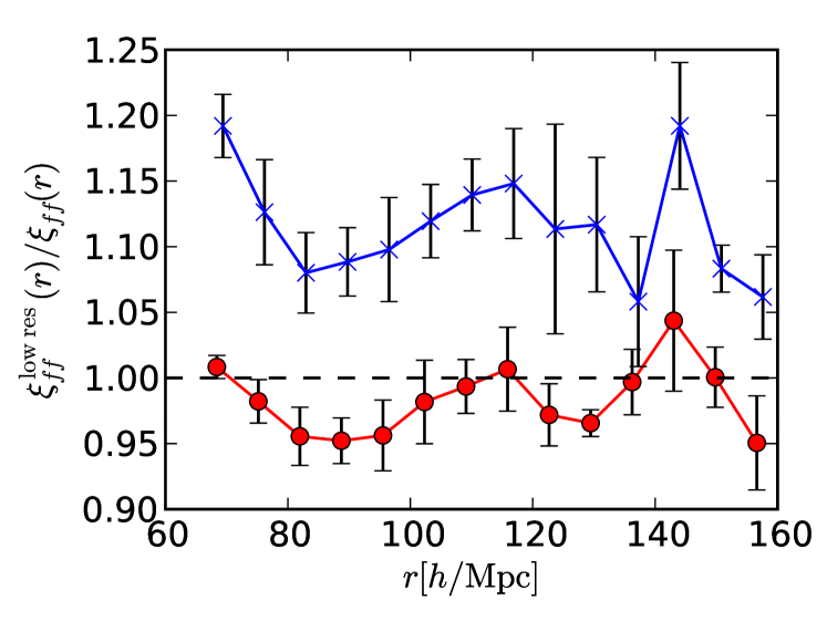
To test the effect of limited resolution on the BAO scale we smoothed the 3D density and velocity fields of two of our simulations by a factor of two or four before computing the skewers. As shown in Fig. 1 the simulations are quite well converged, with the ratio of flux correlation functions agreeing to within 10% for a factor-of-two change in resolution. We expect that the missing small scale physics will have a larger effect on the covariance of the clustering, i.e. the error bars, but we do not currently have enough simulations to make this measurement reliably.

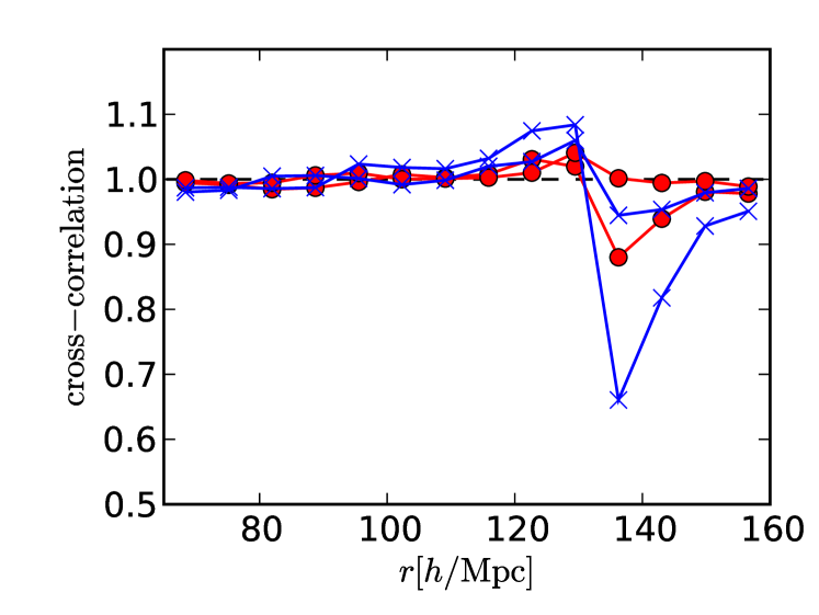
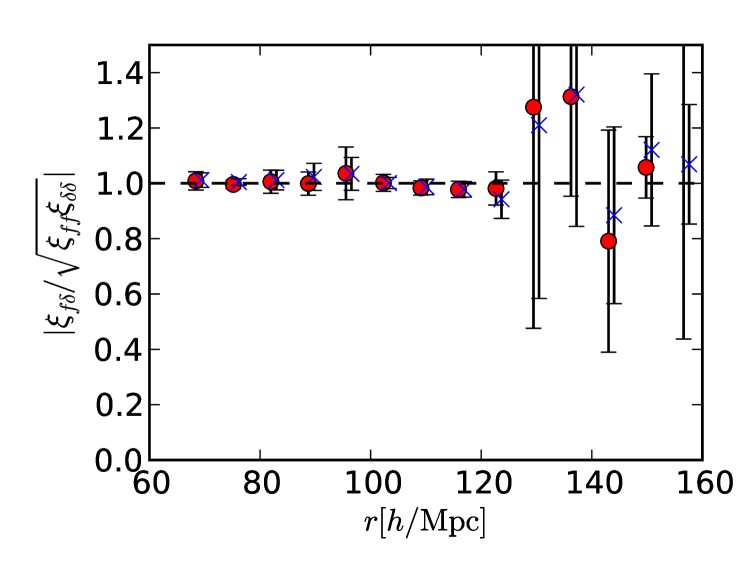
We can also compute the cross-correlation between the flux along the same lines-of-sight in the two simulations with different 3D smoothings of the density and velocity fields. This directly tests the impact of small-scale physics on how well the flux traces the density on large scales. Figure 2 shows this cross correlation. We do not plot the errors, but the uncertainty can be gauged from box-to-box scatter. The correlation is nearly unity on large scales, indicating that the details of the small-scale physics do not alter the behavior of the flux on large scales. The signal becomes difficult to measure beyond $100\,h^{-1}$Mpc where the correlation functions are small and become negative.

Figure 3: The cross power spectrum for the matter overdensity. Filled red points are measured from our simulations, the solid black line is the linear theory prediction, while the blue dashed line is the same for a baryon-less universe.

III BAO signal

Figure 4: The correlation functions, multiplied by $r^{2}$ for easier visualization, as a function of $r_{\perp}$ and $r_{||}$ in $h^{-1}$Mpc. (Top) Correlation functions for matter over-density in real space, redshift space and the theoretical predictions for linear theory. (Bottom) The correlation function in real and redshift space for the flux fluctuations, $\delta_{F}=F/\bar{F}-1$, and (bottom right) the relative difference between the flux and (appropriately scaled) dark matter correlation functions in redshift space $(\xi_{ff}-b^{2}\xi_{\delta\delta})/\xi_{ff}$. The features in this plot follow the crossing of $\xi_{ff}$ through zero, where the quantity we plot diverges. Note that each panel has a very different color scale.

III.1 Fourier space

We start by discussing the signal in Fourier space, where we expect different $k$ modes to be decoupled in the linear regime. Since the signature of BAO in Fourier space is a set of oscillations rather than a single peak, the aliasing of the modes introduced by a finite window function becomes severe in our problem. While this aliasing is most well known from pencil-beam galaxy surveys, it becomes more even more acute in the Lyman-$\alpha$ forest as the data are even more sparsely sampled. In fact, we were unable to obtain a measurement of the three-dimensional flux power spectrum from our skewers, due to strong mixing with the window function. The regular distribution of our skewers likely aggravated the problem, but it would remain even for irregularly distributed skewers.

Figure 5: The monopole correlation function of the dark matter, multiplied by $r^{2}$, in real space (filled red points) and redshift space (blue crosses), the latter divided by $C_{0}$. Error bars are estimated from the box-to-box scatter, are heavily correlated and only indicative of the underlying uncertainties. The linear theoretical prediction is plotted as the (black) solid line.

One can avoid the aliasing issue, however, if one works with cross-power spectra, defined as

$$P_{x}(k,r_{\perp}) = \left\langle\delta_{k,1}\delta^{*}_{k,2}\right\rangle,$$ (1)

$$= \int_{k}^{\infty}\frac{q\,dq}{2\pi^{2}}P(q)\ J_{0}\left(r_{\perp}\sqrt{q^{2}-k^{2}}\right)\,.$$ (2)

where $\delta_{k}$ is the Fourier transform of matter over-density or flux along a single skewer and $r_{\perp}$ is the transverse separation between skewers.

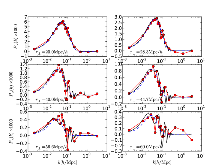
In Figure 3 we show the cross spectrum for the matter overdensity and the corresponding linear predictions for both baryonic and baryon-less universes for a few values of $r_{\perp}$. Note that the acoustic feature not only appears as a series of oscillations superimposed over a smooth shape, but the oscillations have an increasing frequency. Methods which involve measuring binned cross power spectra would need very fine binning to avoid losing signal-to-noise. While the full array of cross-spectra undoubtedly contains the acoustic information, the difficulties of extracting it from this statistics appeared daunting, and we do not consider the cross power spectra any further.

III.2 Configuration space

The configuration space statistics more naturally allow for complex observing geometries, and irregularly sampled data while in principle having more complex covariance properties. We measured the correlation function of both $\delta$ and $\delta_{f}$ in both real and redshift space by brute-force averaging over all possible pairs of pixels in bins of perpendicular distance $r_{\perp}$ and parallel distance $r_{||}$.

In real space, within the context of the peak-background split model one can argue that the two-point flux statics should go as

$$\xi_{ff}(r)=B(r)\xi_{\delta\delta}(r)+A(r),$$ (3)

where $\xi_{ff}$ is the flux correlation function, $\xi_{\delta\delta}$ is that of the matter and $A(r)$ and $B(r)$ are functions that are smooth on large scales. In practice we find that $B(r)$ is a constant and $A(r)$ is consistent with zero in our simulations allowing us to write

$$\xi_{ff}(r)=b^{2}\xi_{\delta\delta}(r)$$ (4)

with $b$ a large-scale bias.

In redshift space, we start by modeling the large-scale redshift space distortions from super-cluster infall as Kaiser (1987)

$$\xi(r,\mu)=\sum_{\ell=0,2,4}\xi_{\ell}(r)\,L_{\ell}(\mu),$$ (5)

where $L_{\ell}(\mu)$ indicates the Legendre polynomial of order $\ell$ and Hamilton (1992)

$$\xi_{0}(r) = C_{0}\xi(r),$$

$$\xi_{2}(r) = C_{2}\left[\xi(r)-\bar{\xi(r)}\right],$$

$$\xi_{4}(r) = C_{4}\left[\xi(r)+\frac{5}{2}\bar{\xi}(r)-\frac{7}{2}\widetilde{\xi}(r)\right],$$ (6)

with

$$C_{0} = 1+\frac{2}{3}\beta+\frac{1}{5}\beta^{2},$$

$$C_{2} = \frac{4}{3}\beta+\frac{4}{7}\beta^{2},$$

$$C_{4} = \frac{8}{35}\beta^{2}$$ (7)

and

$$\bar{\xi}(r) = \frac{3}{r^{3}}\int_{0}^{r}s^{2}\xi_{R}(s)ds$$

$$\widetilde{\xi}(r) = \frac{5}{r^{2}}\int_{0}^{r}s^{4}\xi_{R}(s)ds.$$ (8)

We use $\xi_{R}$ here to explicitly denote the real-space correlation function. These expressions hold for both the matter and the flux, with $\beta=f\equiv d\ln\delta/d\ln a\simeq\Omega_{m}^{0.6}\simeq 1$ in the former case. We leave $\beta$ as a free parameter for the flux, although we expect it to be close to unity also.

Figure 6: (Top) The flux correlation function in real (filled red points) and redshift (blue crosses) space. The black solid and and dashed lines are the scaled matter correlation functions. (Bottom) as above but divided by the equivalent matter linear correlation function. There is no deviation from scale-independent bias seen in the lower panel. Errors are estimated from the box-to-box scatter, are heavily correlated and only indicative of the underlying uncertainties.

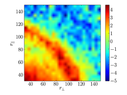
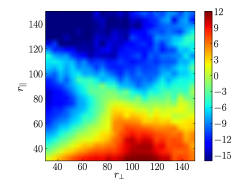
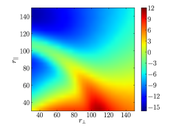
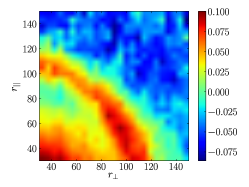
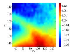
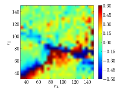
We show our main results in Figure 4, which plots the correlation functions (multiplied by $r^{2}$) in both real space and redshift space, along with theoretical predictions from the simple model described above. The left panels show the real-space correlation function, where one can clearly see the expected BAO ‘ridge’ at $r\simeq 105\,h^{-1}$Mpc. The middle panels show the correlation function in redshift-space, which is very similar to the left panels with the exception of a bias. The Lyman-$\alpha$ flux follows the dark matter and shares the same $\beta\simeq 1$. In the upper right-hand panel we show the predictions calculated using the linear theory correlation function and super-cluster infall with $\beta=0.96$, appropriate to the matter at $z=2.5$.

Our ability to use linear theory to describe the acoustic signature at these redshifts is an important feature of the method. The dominant effect of non-linear clustering is to broaden the acoustic peak, with an amplitude that can be estimated from the rms Zel’dovich displacement Eisenstein et al. (2007b); Crocce and Scoccimarro (2008); Matsubara (2008). At $z=2.5$ this is about $3\,h^{-1}$Mpc in our cosmology, to be compared to the much larger intrinsic width of the acoustic feature (set by the diffusion, or Silk, damping scale: $12\,h^{-1}$Mpc). Adding these in quadrature we see non-linear evolution will only change the peak width by $4\%$. Thus linear theory should accurately describe the acoustic feature in the matter at these redshifts. It is also interesting to note that super-cluster infall does not generate an elliptical contour in redshift space, as can be seen clearly in Eq. (6).

Finally, the bottom right-hand panel of Figure 4 shows the residuals $(\xi_{ff}-b^{2}\xi_{\delta\delta})/\xi_{ff}$ in redshift space. The bright ridge is associated with the correlation function going though zero, which increases the fractional errors, but there is no large-scale radial structure in the difference plot.

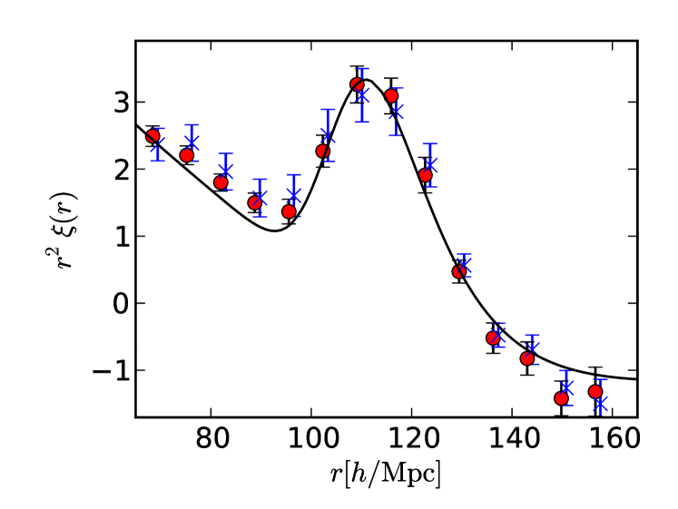
We now focus our attention on the angularly averaged (or monopole) correlation function, $\xi_{0}$, which in the large-scale limit should be proportional to the real-space correlation function (Eq. 6). Figure 5 shows $\xi_{0}$ of the matter in real and redshift space, using only information from the skewers, compared to the linear theory predictions. We note that linear theory describes the matter very well on these scales and at this high redshift in both real and redshift space.

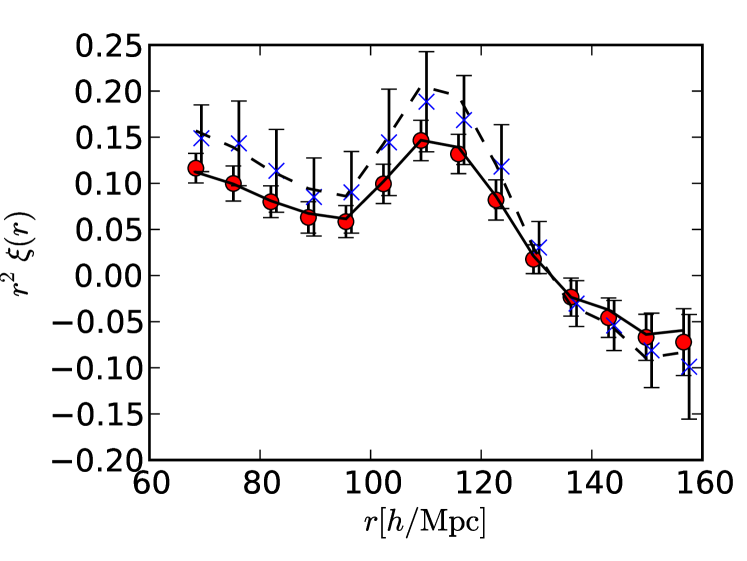
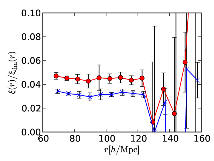
Figure 6 shows the real and redshift space correlation functions of the flux and the ratio of the flux to matter correlation functions (the ‘bias’ squared). The implied bias is consistent with scale-invariant at $b\simeq 0.2$, comparable to that obtained by McDonald (2003). Finally, Figure 7 shows the cross-correlation coefficient between the flux and matter over-density,

$$r\equiv\sqrt{\frac{\xi^{2}_{f\delta}}{\xi_{ff}\xi_{\delta\delta}}}$$ (9)

which is unity when flux traces matter perfectly. While in principle $r\leq 1$, when it is measured from simulations it can exceed unity due to noise. The simulations show that the variations in the flux are tracing those in the matter remarkably well on all scales of interest, in both real and redshift space. This validates the idea of measuring the BAO feature in the Lyman-$\alpha$ forest, and shows that there is no information lost in measuring flux rather than matter fluctuations on these large scales even though the dynamic range in the flux can be drastically smaller than in the density field.

Figure 7: The cross-correlation coefficient between flux and matter over-density in real (filled red points) and redshift (blue crosses) space.

IV Fluctuating photo-ionization rate

While our ability to measure the acoustic scale with galaxies has been impressively demonstrated, we still do not know whether this will be possible from the Lyman-$\alpha$ forest. The calculations above suggest that the signal is present, and the propagation of statistical errors suggest the measurement will be interesting McDonald and Eisenstein (2007), however there are many systematic error which need to be controlled in order to obtain the forecast statistical precision.

One possible cause for concern, in addition to systematic errors in the measurements themselves, is non-gravitational contributions to the flux correlations. These could arise from hydrodynamic forces, radiative transfer effects, reionization heating or other departures from the simple FGPA assumed thus far Meiksin (2007). Many of these effects are expected to contribute mostly on small scales, with no power preferentially on the acoustic scale, and by the arguments provided earlier should not bias the BAO measurement (see e.g. Figure 2). Diagnostics of these non-gravitational contributions can be found in the higher moments of the flux Zaldarriaga et al. (2001); Fang and White (2004) and all indications are that the forest is dominated by gravitational instability on large scales. However, the errors on such measurements are still large enough that the issue is not settled.

One possible contributor to the observed power on large scales is fluctuations in the UV background field or the photo-ionization rate ($\Gamma$). Since the attenuation length of the IGM at $z\sim 2-3$ is large, and the background is thought to be dominated by rare sources (QSOs), $\Gamma$ may have spatial structure on large scales. If the IGM is in photo-ionization equilibrium the optical depth, $\tau\propto\Gamma^{-1}$. Since this is the most obvious source of ‘extra’ large-scale power we investigate this scenario in more detail.

To begin we estimate the expected magnitude of fluctuations in the ionizing background field assuming it is generated by UV light from quasars Meiksin and White (2004); Croft (2004); McDonald et al. (2005). We do this numerically by populating each $(1.5\,h^{-1}{\rm Gpc})^{3}$ box with mock quasars with luminosities following a broken power-law luminosity function

$$\Phi\propto\frac{1}{(L/L_{\star})^{\alpha}+(L/L_{\star})^{\beta}}$$ (10)

with the parameters detailed in Table 5 of Croom et al. (2004). We neglect any luminosity dependent conversion from optical of UV luminosity in this preliminary study. Each QSO is assumed to emit isotropically with constant luminosity $L$, so the contribution to the photo-ionization rate from the $i$th QSO at distance $r_{i}$ can taken to be

$$\Gamma_{i}\propto L_{i}\ \frac{e^{-r_{i}/r_{0}}}{4\pi r_{i}^{2}}$$ (11)

which neglects finite lifetimes or light-cone effects. Here $r_{0}$ is the ’attenuation length’ of the IGM, which is $\mathcal{O}(100\,{\rm Mpc})$. We chose $r_{0}=100\,h^{-1}$Mpc, close to the acoustic scale, to maximize the potential contamination effect Meiksin and White (2004).

Since $r_{0}$ is large, we neglect any QSO clustering in our model, placing the sources at random within the volume. The spatial structure in the photo-ionization rate, or summed UV background, depends on the luminosity function, in particular on the slopes at both the faint and bright end. Table 1 shows some characteristic examples, with the variations in the photo-ionization rate ranging from $31\%$ to $39\%$. In what follows we shall take $0.01\leq L/L_{\star}\leq 100$, $\alpha=-3.31$ and $\beta=-1.09$ as our fiducial model for the QSO component. The correlation function of $\Gamma$ is close to constant at small scales, and falls dramatically beyond the attenuation length, $r_{0}$.

$\alpha$	$\beta$	$M_{\rm lo}$	$M_{\rm hi}$	$\sigma_{\Gamma}/\langle\Gamma\rangle$
-3.31	-1.09	-29	-16	0.37
-3.31	-1.29	-29	-16	0.31
-3.31	-1.09	-29	-20	0.38
-3.31	-1.29	-29	-20	0.32
-3.31	-1.09	-29	-22	0.39
-3.31	-1.29	-29	-22	0.35

Table 1: Relative rms fluctuations in the UV background or photo-ionization rate, $\sigma_{\Gamma}/\langle\Gamma\rangle$, for different choices of the slopes in the QSO luminosity function and the magnitude limits of the QSOs we include.

To the particular realization of the QSO component we add a uniform piece (to model the emission from faint AGN, galaxies and the IGM itself Meiksin (2007)) such that the rms fluctuation of the total is $5\%$, $10\%$ or $20\%$ and divide our original $\tau$ in every pixel by the ionization rate at that location. The overall normalization is rescaled to set the mean flux, $\bar{F}=0.8$.

Figure 8: The effect of photo-ionization rate fluctuations on the flux correlation function. The four panels show correlation functions for UV fluctuations of 0% (top left), 5% (top right), 10% (bottom left) and 20% (bottom right). Note that the vertical scale is different in each panel. The solid lines correspond to the model of Eq. 12.

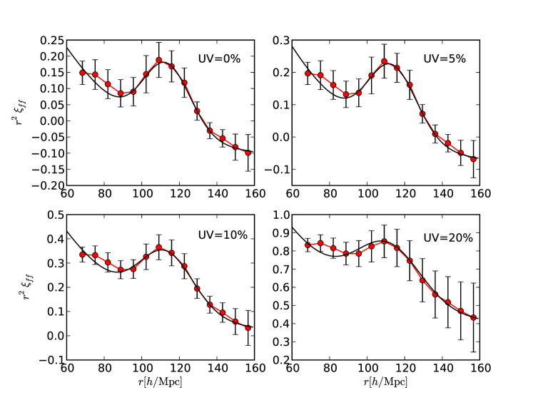
Figure 8 shows the correlation functions of the resulting fluxes. Fluctuations in $\Gamma$ significantly affect the correlation function on large scales, increasing the level of power by a large factor. The additional power is however quite smooth, indicating that the acoustic information is still accessible. To see whether one can still reliably measure the position of the peak in such degraded data, we have attempted to fit the data using the following theoretical model

$$\xi(r)=b^{2}\left(\xi_{\rm nb}(r)+\frac{h}{r^{2}}G(r_{\rm peak},\sigma_{\rm peak})\right)+\mathcal{o},$$ (12)

where $b$, $h$, $r_{\rm peak}$, $\sigma_{\rm peak}$ and $\mathcal{o}$ are free parameters, $\xi_{\rm nb}$ is the linear correlation function for a baryon-less universe, and $G(\mu,\sigma)$ is a Gaussian. We do not advocate this as a realistic model of the correlation function, but merely as a convenient prescription allowing us to asses whether there are any biases introduced in the measurement of the position of the peak by the presence of UV fluctuations. We found best-fit point in each of the 8 boxes individually, assuming a diagonal covariance with the plotted error bars, and used the scatter between these best fits to asses the uncertainty in the parameters. The results of these fits are shown in Table 2 and Figure 8.

model	$r_{\rm peak}$	$\sigma_{\rm peak}$
dark matter, real space	$113.2\pm 1.0$	$16.5\pm 2.5$
flux, redshift space	$113.1\pm 0.6$	$17.9\pm 2.9$
flux, redshfit sp., UV=5%	$113.1\pm 0.6$	$18.6\pm 3.1$
flux, redshift sp., UV=10%	$112.8\pm 0.7$	$20.4\pm 3.0$
flux, redshift sp., UV=20%	$111.1\pm 1.1$	$24.4\pm 4.1$

Table 2: Fits of the correlation function, including UV background fluctuations, to the model of Eq. 12.

These results indicate that the peak position is not affected by the presence of small UV fluctuations, but fluctuations larger than around $\sim 20\%$ start to overwhelm the acoustic signal and biases begin to introduced into the peak position recovery. It is possible that more sophisticated modeling could still recover the peak, but it is likely that such large UV fluctuations will degrade the accuracy of the BAO measurement. In principle one can search for evidence of UV fluctuations in existing QSO spectra. We also find a weak evidence that the width of the peak broadens as UV fluctuations are increased.

V Discussion and Conclusions

Baryon acoustic oscillations have become one of our most promising methods for determining cosmological distances and hence the expansion history of the Universe. The structure in the spectrum of distant quasars, which is thought to trace the structure of the IGM at near mean density, has been suggested as a relatively cheap method for measuring BAO at high redshift White (2003). It is difficult to compute the BAO signal in the Lyman-$\alpha$ forest analytically, since it involves projection of a non-linear mapping of a non-linear density field in redshift space. Instead we have used large-volume N-body simulations. We argued that while the small-scale physics in these simulations is not accurate, the overall picture should not change drastically with more realistic simulations. Our conclusions can be summarized as follows.

We see clear evidence for the acoustic scale in our 180,000 mock spectra. While the BAO signal is present in both Fourier and configuration space statistics, the latter seem to be the better for analyzing the data. There are two mains reasons for this. First, the BAO feature is a single comparably narrow feature in the correlation function, rather than a series of oscillations in the power spectrum. Second, the complex nature by which the Lyman-$\alpha$ forest samples the underlying field makes the analysis considerably more subtle in Fourier space, or conversely the mask much easier to handle in configuration space.

Within the peak-background split approximation, the Lyman-$\alpha$ flux follows the mass fluctuations on large scales. Within the FGPA the flux is a highly non-trivial but deterministic transformation of the underlying density field and we find that the Lyman-$\alpha$ flux correlation functions trace the mass with high fidelity on large scales, with negligible scale dependent bias. We also find that the cross-correlation between the flux and matter is consistent with unity. This is both surprising, given that the flux has limited “dynamic range” compared to the mass, and very encouraging.

Given the difficulty of observing in the deep ultra-violet bands from the ground, Lyman-$\alpha$ observations are limited to redshifts $z>2$ from ground based observations. The upper practical limit is set by the fact that quasars must be bright enough to observe them with a survey instrument and this limits the upper redshift to $z\sim 2-3$. Our simulation redshift of $z=2.5$ is thus at a typical value for a future instrument such as BOSS. Quantitative details are likely to change with redshift, but our main qualitative conclusions are robust, because there is no fundamental change in the properties of the intergalactic medium in the redshift range of interest.

Similarly, our skewers were simulated at a fixed redshift, while the real Lyman-$\alpha$ forest probes an evolving intergalactic medium. This will manifest itself as an effective large-scale bias that evolves with redshift, but is unlikely to change abruptly. We therefore propose to analyse the data in discrete redshift bins that are wide enough to have enough Fourier modes along the line of sight, but are at the same time narrow enough to allow an approximation of a constant or linearly varying effective large-scale bias.

However, a number of other systematic effects will need careful investigation before the BAO program can be carried out with Lyman-$\alpha$ forest data. We have begun by investigating the effect of spatial structure in the photo-ionization field, which modulates the optical depth on scales comparable to the acoustic feature. We find that such a modulation does not introduce any confusion into the determination of the acoustic scale, though it does modulate the total amplitude of the flux correlation function. This is not too surprising, the photo-ionization rate does not know to add power at $105\,h^{-1}$Mpc differently than at $104$ or $106$, but is also encouraging.

As the simulations become increasingly realistic we may begin to see some scale-dependence in the bias. We therefore suggest that one should model BAO in the Lyman-$\alpha$ forest, by measuring a set of bands in the correlation function, together with a linear $\beta$ parameter. This could for example be achieved using an (optimal) quadratic estimator. The resulting $\beta$ should be close to that of the matter, i.e. close to unity. In order to be conservative, the resulting correlation function could be compared with the theoretical predictions for the matter correlation function using the formalism in Equation 3 with $A(r)$ and $B(r)$ being smooth, one or two parameter functions. Sufficiently accommodating functions can also protect against unexpected systematics.

Significantly more work needs to be done before this program can be executed and there are several important effects that need to be understood. First, quasar continuum fluctuations can potentially give rise to large-scale fluctuations that might have a preferred scale. The fact that we are cross-correlating different spectra alleviates the problem to some extent, but may not solve it. Similarly, metal contamination can also give rise to spurious correlations. If fluctuations in the UV background, or photo-ionization rate, are large they may imprint large-scale power in the flux correlation function which can overwhelm the acoustic signal and reduce the sensitivity of the measurement.

Many of these issues can be dealt with using two basic approaches. The first is to model them. For example, pixel pairs which are thought to be contaminated by a metal doublet could be ‘blinded’ within an optimal quadratic estimator. A second method is to split the full sample into all possible subsamples. For example, quasars of the same absolute magnitude or the same source redshift are more likely to have similar continuum fluctuations and one could check the results by splitting the sample into subsamples according to QSO magnitude or redshift. Our results provide added impetus to further develop these promising ideas.