Edinburgh 2009/06
IFUM-941-FT
FREIBURG-PHENO-09/03
Precision
determination of electroweak parameters
and the strange content of
the proton
from neutrino deep–inelastic scattering
The NNPDF Collaboration:
Richard D. Ball1,
Luigi Del Debbio1, Stefano Forte2, Alberto Guffanti3,
José I. Latorre4, Andrea Piccione2,
Juan Rojo2 and Maria Ubiali1.
1 School of Physics and Astronomy, University of Edinburgh,
JCMB, KB, Mayfield Rd, Edinburgh EH9 3JZ, Scotland
2 Dipartimento di Fisica, Università di Milano and
INFN, Sezione di Milano,
Via Celoria 16, I-20133 Milano, Italy
3 Physikalisches Institut, Albert-Ludwigs-Universität Freiburg
Hermann-Herder-Straße 3, D-79104 Freiburg i. B., Germany
4 Departament d’Estructura i Constituents de la Matèria,
Universitat de Barcelona,
Diagonal 647, E-08028 Barcelona, Spain
This paper is dedicated to the memory of Wu-Ki Tung
Abstract:
We use recent neutrino dimuon production data combined with a global deep-inelastic parton fit to construct a new parton set, NNPDF1.2, which includes a determination of the strange and antistrange distributions of the nucleon. The result is characterized by a faithful estimation of uncertainties thanks to the use of the NNPDF methodology, and is free of model or theoretical assumptions other than the use of NLO perturbative QCD and exact sum rules. Better control of the uncertainties of the strange and antistrange parton distributions allows us to reassess the determination of electroweak parameters from the NuTeV dimuon data. We perform a direct determination of the and CKM matrix elements, obtaining central values in agreement with the current global CKM fit: specifically we find and . Our result for is more precise than any previous direct determination. We also reassess the uncertainty on the NuTeV determination of through the Paschos-Wolfenstein relation: we find that the very large uncertainties in the strange valence momentum fraction are sufficient to bring the NuTeV result into complete agreement with the results from precision electroweak data.
1 The strange content of the nucleon
The determination of the strange and antistrange quark distributions of the nucleon is of considerable phenomenological interest, because many final states in the standard model and beyond couple directly to strangeness. A notable example is the determination of the electroweak mixing angle by the NuTeV collaboration [1], which might provide evidence for physics beyond the standard model, and which is very sensitive [2] to the strange content of the nucleon.
Unfortunately, the bulk of the data which are used for parton determination, namely neutral-current deep-inelastic scattering, have minimal sensitivity to flavour separation, and no sensitivity at all to the separation of quark and antiquark contributions. As a consequence, until very recently in standard parton fits such as CTEQ6.5 [3] and MRST2006 [4], the strange and antistrange quark distributions were not determined directly: rather, they were assumed to be equal, and then proportional to the total light antiquark sea distribution. The only available attempt at a determination of the strange and antistrange distributions [5] was based on a re-analysis of old (mostly bubble-chamber) charged-current neutrino-nucleon scattering data: unfortunately, the quality of these old data was insufficient for a reliable determination.
This situation has changed recently, due to the availability of a wider set of inclusive neutrino deep-inelastic scattering data [6, 7] and, more importantly, of data for deep-inelastic neutrino and anti-neutrino production of charm [8, 9, 10] (“dimuon” data, henceforth), which is directly sensitive to the strange and antistrange parton distributions. As a consequence, dedicated analyses of the strange quark distribution have been performed [11, 12, 13, 14], and independent parametrizations of the strange and antistrange distributions are included in most recent parton fits [15]. However, the standard method of parton determination used in all these references, which is based on fitting the parameters of a fixed functional form, is known to be hard to handle when the experiments are relatively unconstraining. Indeed, it is not uncommon that the addition of new experimental information to a parton fit of this kind, actually leads to an increase rather than a decrease of uncertainty bands (see e.g. [16]), because the new data require the use of a more general parametrization. This hampers a direct statistical interpretation of the uncertainty bands on parton distributions obtained in this way: indeed, in some of these parton determinations [15, 17] experimental uncertainties are inflated by suitable “tolerance” criteria. Precision measurements are thus very difficult to obtain whenever the results are significantly affected by parton uncertainties. This is clearly the case in the extraction of the electroweak mixing angle from the NuTeV data of Ref. [1], and it could be more generally an issue for LHC observables which depend crucially on the strange distribution, such as the “standard candle” [17].
A method of parton determination which is free of these difficulties was developed by us in a series of papers [18, 19, 20], and has led recently to the construction of a full parton set based on a fit to a global set of deep-inelastic scattering data: NNPDF1.0 [21]. This method is based on the use of neural networks for parton parametrization, and a Monte Carlo method supplemented by a suitable training and stopping algorithm for the construction of the parton fit. In this approach, parton distributions are given as a Monte Carlo sample representing their probability distributions as inferred from the data: so, for instance, uncertainties can be obtained from the sample by computing standard deviations, likelihood intervals by determining frequency histograms, and so on.
It was shown that this methodology is largely free of bias related to parton parametrization, and it handles in a satisfactory way incomplete information, contradictory data, and the addition of new data within a single framework. In particular, in Ref. [21] it was explicitly verified that when data are removed by changing the kinematic cuts, the uncertainty bands widen in such a way that results before and after the cuts remain compatible, while results outside the data region directly affected by the cuts remain stable. In Ref. [22] it was further checked that the same behaviour is observed when the whole dataset is altered, e.g. by removing all data from one or more experiments: a fit to a smaller dataset has wider uncertainties, but remains compatible with the fit to the larger dataset.
That these stability properties of the NNPDF approach apply also to the way the strange distribution is treated was shown in a dedicated study based on the same methodology [23], leading to the NNPDF1.1 parton set. In NNPDF1.1, the strange parton distributions are parametrized by two independent neural networks, instead of being taken to be proportional to the light antiquark distribution as in NNPDF1.0. However, the dataset is the same as for NNPDF1.0: so the distribution is only very weakly constrained, and the essentially unconstrained by the the data. Nevertheless, when results of this pair of fits are compared, they show remarkable stability, despite the fact that each neural network is parametrized by a very redundant set of parameters (the addition of two neural nets results in the addition of 74 extra free parameters in the fit). Indeed, parton distributions which are unaffected by the addition of independent strange degrees of freedom (such as the gluon) are unchanged, and the only marked effect of the independent parametrization of strangeness is an increase, by about a factor two, of the uncertainty on the total valence quark distribution ( ). Remarkably, statistical analysis of the NNPDF1.0 set alone was already sufficient to show [21] that the uncertainty on this combination was underestimated.
In this paper, by adding recent dimuon data to the global deep-inelastic scattering dataset on which the NNPDF1.0 and NNPDF1.1 fits were based, we construct a new parton set, NNPDF1.2, which includes a determination of the strange and antistrange distributions. Furthermore, we determine directly the and CKM matrix elements which control the strength of the charged–current coupling to neutrinos in dimuon production of the strange and down quarks respectively, and we use our determination of the strange quark distribution to compute the correction to the Paschos-Wolfenstein ratio to be used in extractions of the electroweak mixing angle.
We find that the shape of the strange and antistrange distributions which are compatible with data are rather more general than those obtained in other recent studies [11, 12, 13, 14, 15, 17]. Our uncertainty on the ratio of strange to light sea momenta is rather more asymmetric than hitherto assumed: . This may have nontrivial implications for LHC observables, such as the cross section ratio mentioned above. Despite these increased uncertainties, we find that, perhaps surprisingly, the dimuon data are sufficient to determine . This is one order of magnitude more precise than any other direct determination from neutrino deep-inelastic scattering, and is comparable to the current PDG best average of direct determinations from meson decays, ( [24]), though still two orders of magnitude worse than the results of a global CKM fit. The related CKM element is also determined, , with a similar accuracy to other determinations from dimuon data.
We further find that the distribution, which must change sign as a function of in order for the total nucleon strangeness to vanish, can do so in a wide variety of ways, and that its sign at any given is not well determined. As a consequence, the uncertainty in the strange valence momentum fraction, and thus in the correction to the Paschos-Wolfenstein ratio, is much larger than hitherto assumed, and is such that the NuTeV measurement of is actually in complete agreement with determinations from precision electroweak data once this uncertainty is taken into account.
Many of the techniques and tools that we use in this paper are part of the standard NNPDF methodology, already described in detail in Refs. [19, 20, 21] and used there for the construction of the NNPDF1.0 parton set. Here we will focus on the new aspects of the NNPDF1.2 set, and then discuss our main results. Thus in Sect. 2 we describe the dimuon cross section and its available experimental determinations, and in Sect. 3 we will give its expression in perturbative QCD and thus its relation to the strange distribution, and discuss the way the strange and antistrange distributions are treated, as well as some specific theoretical issues related to the treatment of this observable, such as the treatment of the charm mass and of nuclear corrections. Full details of the hard kernels used to construct the physical observables are given in Appendix A. In Section 4 we present our determination of the strange and antistrange distributions, specifically their shape and their contribution to the nucleon momentum, and compare them to results obtained by other groups. In Section 5 we will discuss in detail the implications of our results for precision electroweak measurements, and discuss specifically the determination of the CKM matrix elements and and the impact of our results on the NuTeV determination of the electroweak mixing angle.
2 Experimental data
The NNPDF1.2 parton determination is based on the same data set used for NNPDF1.0, supplemented by data on deep-inelastic neutrino production of charm from NuTeV [8, 25] which give us a handle on the strange distribution, whose determination is the main goal of this paper. We also add to the data set some recently published measurements of neutral current and charged current deep-inelastic cross sections by the ZEUS experiment based on HERA-II data [26, 27].
An earlier measurement of the dimuon cross section using the same detector (but a different beam-line) was performed by the CCFR collaboration [28]. This previous measurement is significantly less accurate and its compatibility with the NuTeV data is debatable [14, 8]; we will not include it in our fit. A recent measurement of the dimuon cross section has also been performed by the CHORUS collaboration [9]; unfortunately, however, only the results of a leading–order QCD analysis of this data have been published, and not the cross-section data themselves, which therefore cannot be used in our analysis.
The treatment of experimental data in the present fit follows Ref. [21]. In particular, all information on correlated systematics is included in our fit, in that the full covariance matrix is computed including all available correlated uncertainties (including normalization uncertainties).
Below we give more explicit details of the new data and corresponding observables which have been included in the current fit.
2.1 Data set, uncertainties and correlations
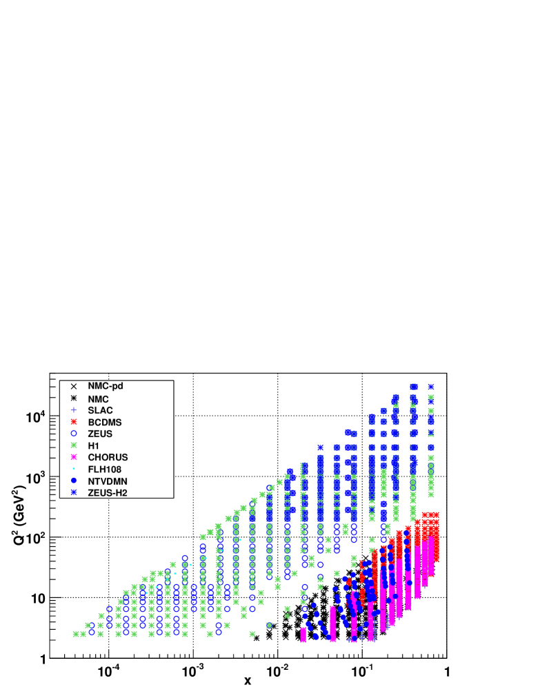
The data set used for the present fit is obtained by supplementing the data set used for the NNPDF1.0 fit, as summarized in Table 1 of Ref. [21], with the data summarized in Table 1 given here. A scatter plot of the full data set is displayed in Figure 1. Note that NuTeV dimuon data overlap with the rest of fixed target experiments, providing information on the proton strangeness for .
| Experiment | Set | (%) | Ref. | ||||||
| ZEUS-HERA-II | |||||||||
| ZEUS06NC | 90 (90) | .005 | 0.65 | 200.0 | 30000.0 | 2.6 | [26] | ||
| ZEUS06CC | 37 (37) | .015 | 0.65 | 280.0 | 30000.0 | 14 | [27] | ||
| NUTEV Dimuon | |||||||||
| NuTeV Dimuon | 45 (43) | .0267 | 0.37 | 1.1 | 116.5 | 19 | [25] | ||
| NuTeV Dimuon | 45 (41) | .021 | 0.25 | 0.8 | 68.3 | 23 | [25] | ||
| Total (including Tab. 1 of Ref. [21]) | 4165 (3372) | ||||||||
The covariance matrix is computed for all the data included in the fit, as discussed in Ref. [21]. The NuTeV dimuon data are affected by a common normalization uncertainty of 2.1% [6]; eight correlated systematics; and a statistical uncertainty. The statistical uncertainty is around 15% for neutrino and around 25% for anti-neutrino data, while correlated systematics are generally smaller by a factor between three and five. This dominant statistical uncertainty is affected by a bin by bin correlation due to the unfolding procedure used in extracting the dimuon cross section from the measured observable. The covariance matrix which describes these correlations is not available. Its effect has been summarized in Ref. [25] by providing for each bin an “effective number of degrees of freedom”, which provides the expected value of the best-fit to the given data bin, i.e., effectively, a rescaling for the statistical error. These rescaling factors can be as low as 30%, and are typically around 50%, indicating sizable correlations.
Rescaling of statistical errors in order to account for missing correlations could bias the fit in an unpredictable way and it is a dangerous procedure if the information on the covariance matrix is lost. On the other hand, only including correlations for the subdominant systematic errors could lead to an underestimate of the relative impact of these uncertainties. Hence, because the covariance matrix of the NuTeV data is unfortunately unavailable, the only consistent procedure for the treatment of these data is to add all uncertainties in quadrature, and only consider normalizations as correlated uncertainties. This is the procedure that we shall follow.
| Experiment | ZEUS-HERA-II | NuTeV Dimuon | Total |
|---|---|---|---|
| -4.2 | -5.4 | -2.3 | |
| 0.999 | 0.999 | 0.999 | |
| 6.5 | -2.6 | -6.1 | |
| 13.79% | 21.23% | 11.24% | |
| 13.88% | 21.17% | 11.24% | |
| 0.999 | 0.998 | 0.999 | |
| 0.287 | 0.034 | 0.146 | |
| 0.294 | 0.034 | 0.146 | |
| 0.994 | 0.978 | 0.996 | |
| 6.89 | 0.169 | 1.61 | |
| 7.03 | 0.168 | 1.54 | |
| 0.997 | 0.988 | 0.988 |
2.2 Observables, kinematic cuts and pseudo-data sample
The set of observables considered in these fits consists of the structure functions and reduced cross-sections considered in Ref. [21] and summarized in Table 1 of that reference, supplemented by the dimuon cross section. Neutrino dimuon production is induced by charm production through charged current interactions of neutrinos with the target nuclei, followed by the fragmentation of the charm quark into a charmed hadron and its decay into a muon. The corresponding cross section is given by
| (1) | |||||
where
| (2) |
The charm production cross section is obtained from the published NuTeV neutrino dimuon production cross sections [25] as
| (3) |
where is the average branching ratio of charmed hadrons into muons and is a bin-dependent experimental acceptance correction. Acceptances are provided by the NuTeV collaboration, based on a leading-order model [29]; next-to-leading order acceptances [30] (not publicly available) differ by less than 3% from the leading-order ones. The branching ratio used in the NuTeV analysis [10] comes from a reanalysis of the emulsion data of the FNAL E531 experiment and turns out to be , in agreement with other determinations [31, 9]. A simultaneous extraction of this parameter along with the determination of strangeness in Ref. [14] leads to a similar result. In the determination of the dimuon cross section, the branching ratio will be set equal to the central value used in the NuTeV analysis [10]. The associated uncertainty will then be included in our fit as discussed in Section 3.2 below.
Our data set is obtained by imposing on all the data listed in Table 1 of Ref. [21] and in Table 1 the same kinematical cuts as in NNPDF1.0, namely GeV2 and GeV2. After these cuts, 84 out of the 90 NuTeV dimuon data points are left. After cuts, the total number of data points in the NNPDF1.2 analysis is .
Error propagation from the experimental data to the fit is performed through a Monte Carlo procedure, described in detail in Ref. [21], by generating a set of 1000 pseudo-data replicas, whose faithfulness can be verified by studying suitable statistical estimators. The statistical estimators for the new data sets included in the present fit, as well as for the global data set, are summarized in Table 2.
3 Neural networks, parton distributions and physical observables
Physical observables are determined from a set of PDFs given at a reference scale, which are in turn parametrized in terms of neural networks, according to the formalism discussed in detail in Sect. 3-4 of Ref. [21]. Here we summarize the new features of this determination: the use of an independent parametrization for the strange and antistrange distribution and its construction in terms of neural networks, the new physical observables used for dimuon data, and some issues that require reconsidering when dealing with this observable, namely the treatment of the charm mass and nuclear corrections.
3.1 Parametrization of the strange PDF
In the NNPDF1.0 fit of Ref. [21], parton distributions were parametrized using five independent neural networks: four independent linear combinations of the two light flavours and anti-flavours, and the gluon. The strange and antistrange quark distributions were assumed to be given by with , and heavy quarks were generated dynamically, using a zero-mass variable flavour number scheme (ZM-VFN). In the subsequent NNPDF1.1 fit [23], two further neural networks were introduced to parametrize the strange and antistrange quark distributions. Here, as in Ref. [23] we parametrize parton distributions in terms of seven independent neural networks, as we now discuss.
The primary partonic quantities out of which all physical observables are built up are the gluon, the singlet quark distribution, the total valence quark distribution, and ten nonsinglet combinations of the valence ) or total () quark and antiquark distribution for the -th quark flavor. These are constructed as in Ref. [21], to which we refer for more details. The starting scale is chosen at the charm threshold, where the charm distributions are assumed to vanish, and the remaining six light quark distributions and the gluon distribution are parametrized in terms of independent neural networks. The possibility of introducing an intrinsic charm distribution will not be studied in the present fit, though there is no obstacle to including it in future studies.
The four light non-strange distributions and the gluon distribution are parametrized in terms of neural networks as in Ref. [21], by letting
| (4) |
where is a linear combination of parton distributions, and NN is a multi-layer feed-forward neural network with two intermediate layers and architecture 2-5-3-1, parametrized by 37 free parameters (weights and thresholds). The constants are either simply set to one, or else used to enforce the valence and momentum sum rules.
The preprocessing function is included in order to speed up the convergence of the fit: the neural network only has to fit the deviation from the behaviour of the preprocessing function, whose exponents are thus fixed to values which absorb some of the gross behaviour of the function without biasing the result (i.e. without imposing a steep growth or fall which would have trouble in reabsorbing). Independence of the results on the choice of the preprocessing exponents was verified in Ref. [21] by varying them within a reasonable stability range. This stability range is identified in Ref. [21] by requiring the quality of the fit to be unchanged as the exponents are varied. A small residual dependence on the preprocessing exponents was found in Ref. [21] for the triplet and total valence quark distributions. In order to be able to disentangle accurately the strange contribution it is important that uncertainties on all light quark flavours are estimated as precisely as possible: for this purpose, in the NNPDF1.1 fit of Ref. [23] and in the present fit all preprocessing exponents are randomized: a different value is taken for each Monte Carlo replica, uniformly distributed within the stability range.
The choice of linear combinations of the two lightest flavours which are parametrized independently according to Eq. (4) is the same in the present fit as in NNPDF1.0. On top of them, we add two independent neural networks in the strange sector, in order to parametrize
| (5) |
according to
| (6) | |||||
| (7) |
where
| (8) |
The exponents , of the preprocessing functions are randomized as discussed above, and their ranges are also listed in Table 3.
The contribution in Eq. (7) is introduced in order to enforce the strange valence sum rule: the constant is fixed by requiring
| (9) |
which gives the condition
| (10) |
Clearly, the sum rules requires to change sign at least once. This way of implementing the sum rule is designed in order to ensure that this crossing happens naturally in the valence region, rather than in some contrived way outside the data region where the shape of is completely unconstrained. To this purpose, the exponents are chosen in such a way that peaks in the valence region, and that the small and large behaviour of are not controlled by the contribution. In practice the latter condition is enforced by requiring and , while the former is enforced by letting , which sets the maximum of at . We then choose , and take as a uniformly distributed random number in the range . The consequences of this very flexible implementation of the strangeness valence sum rule will be discussed in Sect. 4.4 below.
3.2 The dimuon physical observable
The NNPDF1.2 data set, displayed in Fig. 1, contains data for the same set of observables discussed in Ref. [21], with the addition of the dimuon cross section Eq. (1). The latter is determined by the charm structure functions , and , which in the quark model are given by
| (11) | |||
| (12) |
with . Full expressions for these structure functions in perturbative QCD at any scale in terms of the basis of PDFs used in our fits are given in Appendix A.
Because they are not inclusive with respect to the final state quark flavour, these structure functions depend on CKM matrix elements. These are extremely well determined by current global fits including unitarity constraints; for our global fits we will use the current best-fit PDG [24] values: uncertainties on them are tiny and will be neglected. In Section 4 we will then study the quality of our fit as the parameters and are varied without the unitarity constraint, and use this to provide a direct determination of these parameters from the dimuon data.
Also, as already discussed in Sect. 2, the dimuon cross-section Eq. (3) depends on the branching ratio . The uncertainty in this is actually rather significant: in previous analyses [10, 14] of dimuon data this turned out to be one of the dominant sources of uncertainty. To take account of this uncertainty, the value of the branching ratio used in the fit has been randomized about its central value, analogously to the procedure used for the preprocessing exponents, with a Gaussian distribution of width equal to the stated uncertainty [10].
3.3 Treatment of the charm mass
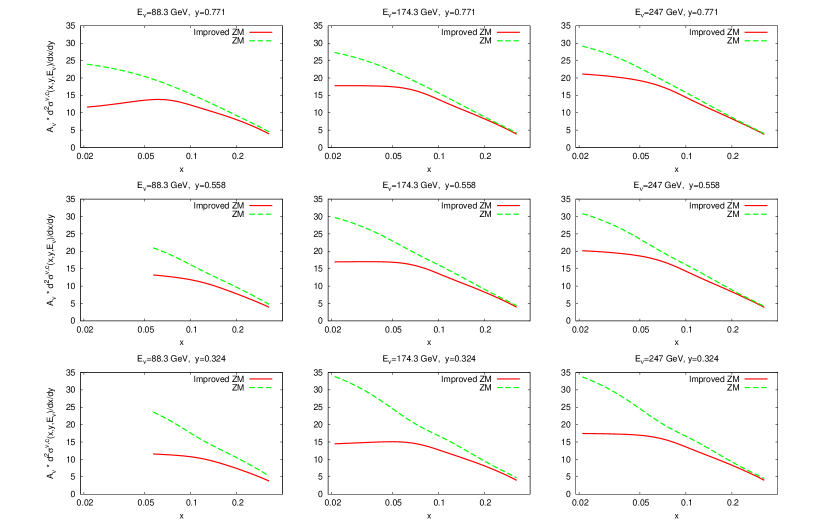
In the previous NNPDF1.0 and NNPDF1.1 parton determinations, heavy quarks were treated in a zero mass variable flavour number (ZM-VFN) scheme, as discussed in Sect. 3.4 of Ref. [21]. Contributions suppressed by powers of the heavy quark mass, i.e. of order , which are neglected in this scheme, have a small but not entirely negligible impact [32], mostly through the initial condition on the charm distribution, which then affects all other PDFs due to the momentum sum rule. For the purpose of the present analysis, an improved treatment of the charm mass is advisable at least for dimuon production, as the dimuon cross section measures charm production, and a sizable fraction of the NuTeV dimuon data are thus at scales close to the charm mass.
To this purpose, we employ (for the dimuon observable only) the improved ZM-VFN (I-ZM-VFN) scheme, proposed in Ref. [33] and discussed in detail in Ref. [34]. There, it was shown that the bulk of the charm mass effects near threshold can be accounted for by requiring that the threshold for the inclusion of heavy quarks in the sum over final states be set at its physical value , and that the phase-space constraint due to the heavy quark mass be respected in convolution integrals. The latter requirement is in practice implemented by replacing the Bjorken variable by a rescaling variable defined as
| (13) |
Whereas results obtained with this I-ZM-VFN scheme are in fair agreement with those obtained with a full treatment of the quark mass (so-called general mass, or GM scheme), and in rather better agreement with the data, they may lead to an excessive suppression of heavy quark production: to this purpose, in Ref. [34] a one-parameter family of rescaling variables has been constructed, such that the agreement with the GM scheme can be optimized by tuning this parameter. It turns out, however, that the simplest choice Eq. (13) is actually very close to the optimal one for charged current deep inelastic scattering.
Hence, in the present analysis we will use the ZM-VFN for all inclusive observables, but for the dimuon cross section Eq. (3) we will use the I-ZM-VFN of Ref. [33]. In practice, this means that we will retain the full dependence in Eq. (1), and in the expressions for the structure functions Eq. (A) all convolutions are defined as
| (14) |
The impact of this treatment of the charm mass is shown in Fig. 2, where we compare a NLO determination of the dimuon cross section Eq. (3) within the ZM-VFN and I-ZM-VFN schemes, based on our previous NNPDF1.0 parton set. The suppression of the cross section at small due to finite quark mass is apparent from this plot. Clearly, the inclusion of quark mass effects only in the determination of the dimuon cross section, and then in the I-ZM-VFN scheme, is an approximation. This approximation will lead to a systematic uncertainty in our determination of the strange PDFs and of CKM matrix elements in the next sections. We will estimate this uncertainty by comparing results obtained in the ZM-VFN and I-ZM-VFN scheme: as the full GM scheme is actually in between these two, this provides a rather conservative overestimate of the associated uncertainty. We will then see that this systematic uncertainty is actually small in comparison to the statistical uncertainty on strangeness and associated observables.
3.4 Nuclear Corrections
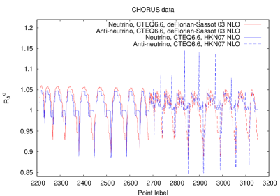
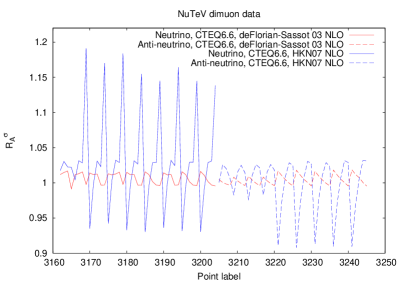
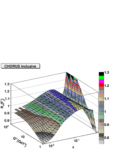
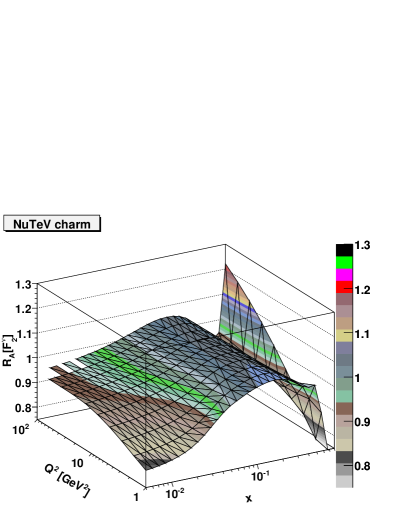
Neutrino data are obtained from deep-inelastic scattering off a nuclear target: for NuTeV essentially Fe, [25], and for CHORUS (whose inclusive structure function measurements are also included in our data set) Pb, , [7]. Therefore, a suitable nuclear correction should be introduced in order to obtain from these data a determination of the PDFs of free nucleons.
Nuclear corrections have been determined by various groups [35, 36, 37, 38], using models of nuclear structure. The correction
| (15) |
to the reduced cross sections and , obtained using the parametrizations of Refs. [35, 36], are displayed in Figs. 4 for the experimental CHORUS inclusive and dimuon NuTeV data. It is apparent that corrections obtained using different models can be significantly different, but they are all quite small. For this reason, nuclear corrections were not used in the NNPDF1.0 fit [21]. In the NNPDF1.2 fit presented here we will not include nuclear corrections in our baseline fit, but, in order to determine the associated systematic uncertainty, we will repeat the fit with the nuclear corrections computed using the models of Refs. [35, 36], which provide corrections to the parton distributions. The dependence of the nuclear correction on the kinematic variables is shown in Fig. 4 in the kinematic region and for values relevant for CHORUS and NuTeV data, using the model of Ref. [37], which instead provides directly a correction to the structure function.
4 Results
In this section we present the NNPDF1.2 parton set. After discussing the general features of the fit and its result, and comparing these to the previous NNPDF parton set, we discuss in detail the determination of the strange and antistrange distributions, which are the novel features of this fit. We finally compare results to experimental data, including a comparison with the recent [26] determination of the structure function.
4.1 The NNPDF1.2 parton set: statistical features
| 5000 | 1/3 | 120 | 3 | 10 |
We have produced a set of replicas of seven PDFs, each determined as an optimal fit to one of the Monte Carlo replicas obtained from the data set of Sect. 2. We have used the genetic algorithm minimization and a cross-validation method for the determination of the optimal fit, according to the method presented in Sect. 4 of Ref. [21]. The parameters of the genetic algorithm are summarized in Table 4; they coincide with those used in Ref. [21] for the five PDFs already present in that fit.
The general statistical features of our final parton set are summarized in Tables 5-6, to be compared with the corresponding tables (Tables 7-8) of Ref. [21], where all the relevant quantities are defined (note that average uncertainties are now given in percentage value, while they were given as absolute values in Ref. [21]).
The statistical features of the fit can be summarized as follows:
-
•
The general features of the total fit (Tab. 5) are essentially indistinguishable from those of Ref. [21], and the comments we made then still apply. The same is true for the features of the fit to individual experiments (Tab. 6) when these were already included in the dataset of Ref. [21]. This stability upon the addition of two new independent PDFs (thus 74 extra free parameters) and a randomization of the preprocessing exponents supports the reliability of the results obtained in NNPDF1.0 for all PDFs which were determined there.
-
•
The quality of the fit to the new HERA II data is comparable to that to the BCDMS data, and somewhat worse than that of the fit to other HERA data. These new data mostly probe the large region, like BCDMS and unlike other HERA data (see Fig. 1), and are generally rather precise, also like BCDMS and unlike other HERA data (see Tab. 1 and Tab. 1 of Ref. [21]). This somewhat larger value of the for large high precision data, though compatible with statistical fluctuations and with the theoretical error related to the use of NLO perturbation theory, may suggest some minor data incompatibility in this region.
-
•
The of the fit to dimuon data is rather smaller than one. This is a consequence of the fact that, as discussed in Sec. 2.1, correlations have not been included for these data because the covariance matrix is not available. The average value of the we obtain is in good agreement with that expected on the basis of the “effective number of degrees of freedom” published in Ref. [25], and with other fits to the same data [14].
-
•
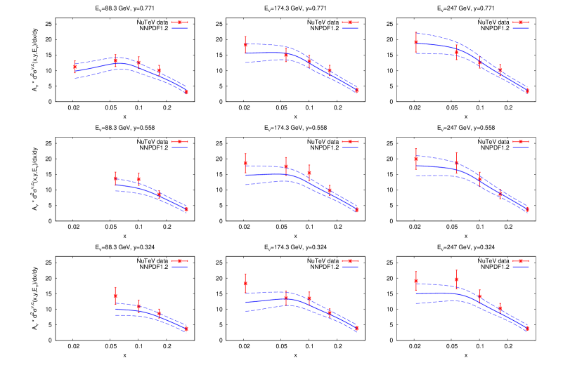
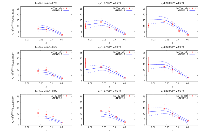
The uncertainty of the fit to dimuon data, as measured by the average standard deviation is very close to the uncertainty of the data, unlike that of all other data sets (reflected by the results for the total fit), where the fit uncertainty is much smaller than the data uncertainty (4% vs. 11% for the total fit). This is a consequence of the fact that dimuon data have little redundancy, and are sensitive to strangeness, to which other data are essentially insensitive; while all other data have a very large redundancy, especially low- HERA data which depend mainly on the quark singlet and gluon. This effect can also be observed in the comparison between experimental data and NNPDF1.2 predictions of Fig. 15.
-
•
The average correlation is very low for the dimuon data, because the only correlated systematics is normalization. However, the fit to these data does display a correlation of the same order of magnitude as for other data, reflecting the underlying smoothness of parton distributions.
| 1.31 | |
|---|---|
| 2.80 | |
| 2.75 | |
| 2.80 | |
| 1024 | |
| 11.0% | |
| 4.0% | |
| 0.15 | |
| 0.32 | |
| Experiment | ||||||||
|---|---|---|---|---|---|---|---|---|
| SLAC | 1.27 | 3.32 | 4.2% | 2.6% | 0.31 | 0.63 | ||
| BCDMS | 1.57 | 3.14 | 5.7% | 4.5% | 0.47 | 0.51 | ||
| NMC | 1.70 | 3.09 | 4.9% | 2.3% | 0.16 | 0.62 | ||
| NMC-pd | 1.46 | 3.12 | 1.7% | 1.7% | 0.36 | |||
| ZEUS | 1.07 | 2.64 | 13% | 3.9% | 0.26 | |||
| H1 | 1.03 | 2.52 | 12% | 3.3% | 0.25 | |||
| CHORUS | 1.37 | 2.88 | 15% | 3.7% | 0.27 | |||
| FLH108 | 1.67 | 2.56 | 72% | 5.7% | 0.65 | 0.76 | ||
| NuTeV Dimuon | 0.62 | 2.62 | 21% | 22% | 0.03 | 0.50 | ||
| ZEUS-HERA-II | 1.51 | 2.90 | 14% | 2.5% | 0.29 | 0.34 |
4.2 The NNPDF1.2 parton set: parton distributions
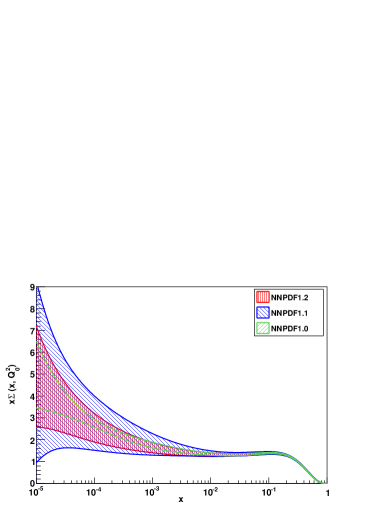
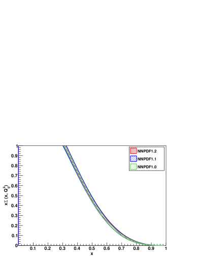
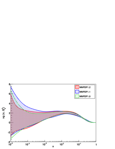
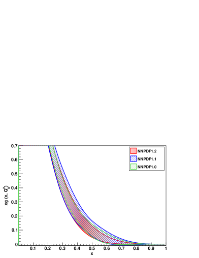
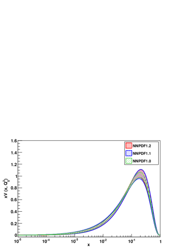
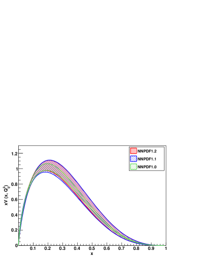
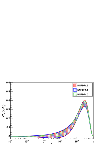
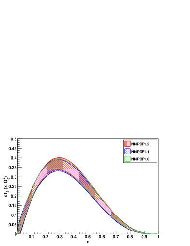
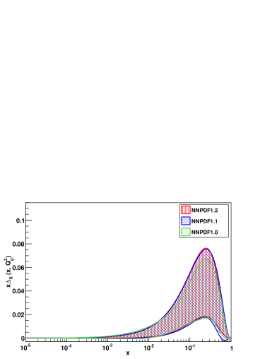
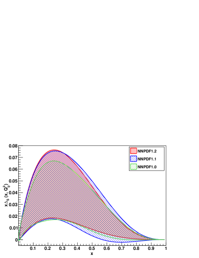
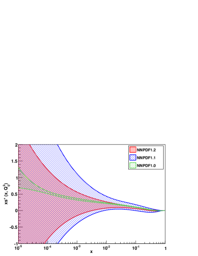
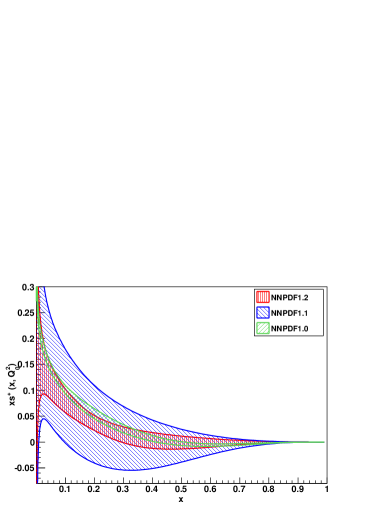
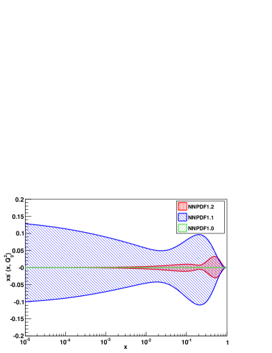
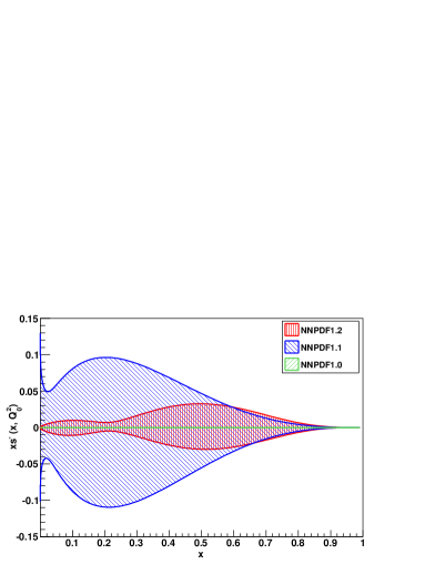
The NNPDF1.2 set of parton distributions at the starting scale GeV2 is displayed in Figs. 5-7, and compared to the previous sets NNPDF1.0 [21] and NNPDF1.1 [23]. The distances (defined as in Ref. [21]) between each pair of these three sets are shown in Table 7.
The general features of this PDF set and its comparison to the previous NNPDF sets are the following
-
•
In the singlet sector, there is very little difference in central values and uncertainties between the NNPDF1.2 and NNPDF1.0 parton sets: the distance between the sets is compatible with statistical fluctuations. The NNPDF1.1, which had an independent parametrization for the strange distribution without any data to constrain it displays an increase in the uncertainty of the quark singlet due to this unconstrained strange contribution.
-
•
The isospin triplet and the sea asymmetry are the same in all NNPDF sets within fluctuations. The total valence has the same central value in all sets within fluctuations, and the same uncertainty in the NNPDF1.2 and NNPDF1.1 sets, while the uncertainty on it was somewhat underestimated in NNPDF1.0. This underestimate of the NNPDF1.0 valence uncertainty was already singled out based on a statistical stability analysis in Sect. 5.4 of Ref. [21], where it was suggested that it could be cured by a randomization of the preprocessing exponents in Eq. (4). This randomization has been implemented in NNPDF1.1 and NNPDF1.2, which indeed have somewhat larger valence uncertainty, compatible with each other. This is despite the fact that the strange contribution to the total valence is affected by a much larger uncertainty in NNPDF1.1 than in NNPDF1.2.
-
•
The central value and uncertainty on the strange distributions Eq. (5) are compatible with those of NNPDF1.1, where strangeness was independently parametrized but essentially unconstrained by data, whereas they are incompatible with those of NNPDF1.0, where strangeness was determined by the assumptions and . This means that this simple assumption, though perhaps not too far off, is insufficient to determine the strange distribution within its stated accuracy. This conclusion was also reached recently in Ref. [13]. The uncertainty on strangeness as we determine it here turns out to be rather larger than that induced by the NNPDF1.0 assumption, but much smaller than that obtained in NNPDF1.1 in the absence of dimuon data. It is thus possible to determine the shape of with reasonable accuracy. However, our determination of turns out to be compatible with the NNPDF1.0 assumption that . We shall discuss the features of the strange distribution in greater detail in Sect. 4.4 below.
| NNPDF1.2 vs. NNPDF1.1 | ||
|---|---|---|
| Data | Extrapolation | |
| 2.7 | 1.2 | |
| 3.1 | 1.8 | |
| 2.4 | 2.0 | |
| 1.3 | 1.4 | |
| 1.5 | 0.9 | |
| 1.1 | 1.2 | |
| 1.1 | 1.0 | |
| 1.3 | 1.4 | |
| 0.8 | 0.8 | |
| 1.3 | 1.1 | |
| 2.0 | 1.6 | |
| 4.5 | 1.8 | |
| 1.1 | 1.3 | |
| 6.1 | 4.6 | |
| NNPDF1.1 vs. NNPDF1.0 | ||
|---|---|---|
| Data | Extrapolation | |
| 1.6 | 0.9 | |
| 4.0 | 2.3 | |
| 2.3 | 1.7 | |
| 1.6 | 1.2 | |
| 1.6 | 0.8 | |
| 1.8 | 3.4 | |
| 1.8 | 1.7 | |
| 5.3 | 5.2 | |
| 1.2 | 1.0 | |
| 1.6 | 1.1 | |
| 1.0 | 1.0 | |
| 5.4 | 2.3 | |
| 1.1 | 1.3 | |
| 7.4 | 4.6 | |
| NNPDF1.2 vs. NNPDF1.0 | ||
|---|---|---|
| Data | Extrapolation | |
| 3.2 | 1.9 | |
| 2.9 | 3.3 | |
| 1.7 | 0.9 | |
| 1.6 | 1.3 | |
| 1.1 | 1.0 | |
| 2.0 | 3.2 | |
| 2.6 | 2.4 | |
| 5.3 | 4.9 | |
| 1.4 | 0.9 | |
| 1.5 | 1.2 | |
| 6.2 | 3.7 | |
| 5.7 | 3.8 | |
| 1.3 | 1.2 | |
| 6.8 | 6.5 | |
4.3 Theoretical uncertainties
As discussed in Sects. 3.3-3.4, dimuon data are potentially sensitive to the treatment of the quark mass, and neutrino data in general are potentially sensitive to nuclear corrections. In order to explore this sensitivity, we have repeated the NNPDF1.2 fit using also for dimuon data the ZM-VFN scheme (as in Ref. [21]) instead of the improved I-ZM-VFN quark mass treatment discussed in Sect. 3.3 and used for the default NNPDF1.2 fit (the ZM-VFN is used for all other data anyway). The distances between results thus obtained are displayed in Tab. 8. It is apparent that there is a certain change in the central value of the strange distribution in the region of the data, of order of about ten, which, with replicas, means that the central value has moved by about in units of the standard deviation. The uncertainty on itself, and the central value of the singlet distribution in the region of the data are affected to a lesser extent, while all other PDFs are unaffected. Thus the charm mass corrections displayed in Fig. 2 have a small but noticeable effect on the determination of the total strange distribution. Our approximate treatment will correspondingly be a source of systematics, which we shall take into account when discussing quantities related to strangeness.
In order to study the sensitivity to the nuclear corrections displayed in Fig. 3 we have repeated the NNPDF1.2 fit with all neutrino data corrected for nuclear effects according to the models of de Florian-Sassot [35] and HKN07 [36]. The distances tabulated in Tab. 8 show that the effect of nuclear corrections is negligible: fits with or without nuclear corrections differ by an amount which is compatible with statistical fluctuations.
| ZM | De Florian-Sassot | HKN07 | ||||
| Data | Extrapolation | Data | Extrap. | Data | Extrap. . | |
| 5.2 | 1.0 | 2.3 | 1.4 | 2.3 | 0.9 | |
| 2.5 | 1.6 | 1.5 | 1.2 | 1.2 | 1.1 | |
| 1.4 | 1.5 | 1.2 | 1.0 | 1.4 | 1.1 | |
| 1.8 | 1.5 | 1.2 | 1.2 | 1.2 | 1.4 | |
| 1.4 | 2.0 | 1.3 | 1.0 | 1.0 | 1.0 | |
| 2.9 | 0.9 | 1.4 | 1.5 | 1.1 | 1.1 | |
| 1.2 | 1.2 | 1.3 | 1.2 | 0.8 | 0.7 | |
| 1.5 | 1.1 | 1.3 | 1.5 | 1.3 | 0.9 | |
| 2.1 | 2.3 | 0.8 | 1.0 | 1.1 | 1.0 | |
| 1.1 | 1.1 | 1.2 | 1.3 | 1.0 | 1.3 | |
| 9.4 | 1.1 | 2.1 | 1.5 | 1.6 | 1.1 | |
| 3.4 | 1.6 | 1.5 | 1.0 | 1.5 | 1.0 | |
| 0.9 | 0.9 | 1.0 | 1.1 | 1.3 | 1.1 | |
| 1.4 | 1.2 | 1.0 | 1.0 | 1.4 | 0.9 | |
4.4 Determination of the strange distribution
The determination of the strange and antistrange PDFs is problematic because of the scarceness of the experimental information on these quantities, which makes it difficult to separate the genuine information from theoretical bias, a situation which our methodology is especially suited to deal with. In previous parton fits, a range of possible shapes of the strange PDFs was explored by assuming different functional forms and studying the variation of results [13].
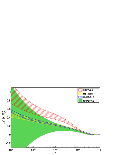
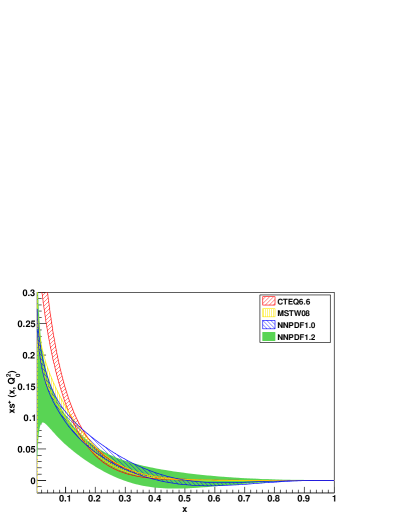
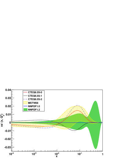
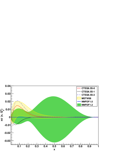

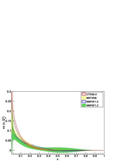
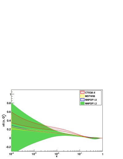
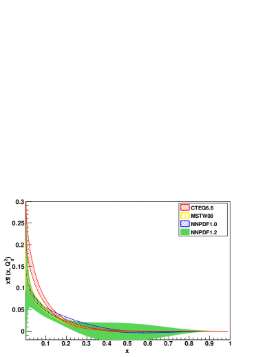
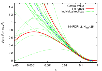
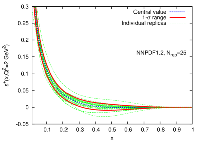
The , and strange PDFs Eq. (5) are shown at the input scale in Fig. 8, where they are also compared to the most recent CTEQ6.6 [17] and MSTW08 [15] sets. Whereas the CTEQ collaboration has not performed a full determination of the uncertainty band, a study of the dependence of the best-fit on assumptions on its functional form was performed in Ref. [13]: several of the corresponding results are also shown in Fig. 8. For greater clarity, in Fig. 9 we also plot the uncertainties on these PDFs.
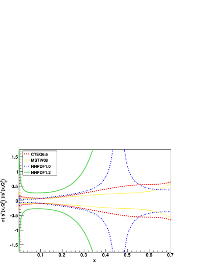
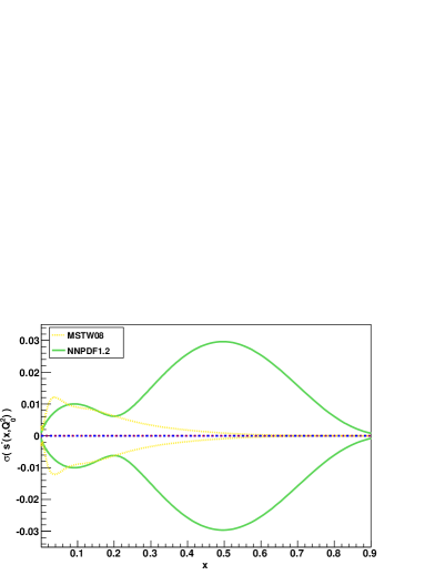
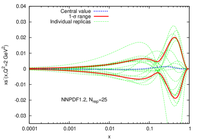
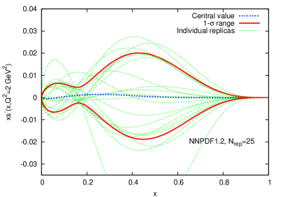
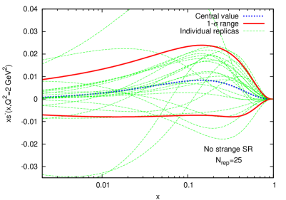
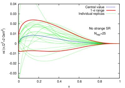
In the data region all determinations of agree, however the NNPDF1.2 has a much larger uncertainty than other existing determinations. The origin of this can be understood by looking at Fig. 10, where we display 25 randomly chosen replicas out of our full set, and the mean and standard deviation computed from them: clearly, our large uncertainty is a consequence of the great flexibility afforded by the neural network parametrization. This is particularly noticeable in the case of , which must have at least one node because of the sum rule Eq. (9): individual replicas cross the –axis in different places, with different sign (from positive to negative or conversely), and some replicas have more than one crossing. It is interesting to observe that the “neck” in the uncertainty on around corresponds to the value of at which the crossing is most likely to occur. The role played by the valence sum rule Eq. (9) in determining these features of the strangeness asymmetry can be elucidated by repeating the fit without imposing it. The results, displayed in Fig. 11, show that even without the sum rule constraint many replicas still cross the the –axis.
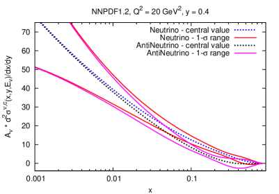
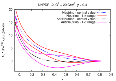
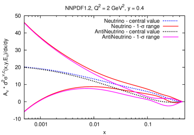
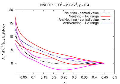
Another theoretical constraint which may help in reducing uncertainties is that of positivity of cross sections. For instance, as in Ref. [21], in the determination of the NNPDF1.2 PDF set we have imposed positivity of the structure function at low and , which helps in reducing the uncertainty of the gluon distribution at the edge of the HERA data region. In view of the fact that (see Fig. 8) both and can turn negative to within one sigma for , and also in the large region, one may wonder whether imposing positivity of the dimuon cross section might likewise help in reducing the uncertainty on the strange and antistrange distributions. In order to test this, in Fig. 12 we display the total dimuon cross section, both at the initial GeV2 and at the typical scale of the NuTeV data GeV2, computed using the NNPDF1.2 PDFs of Fig. 8. The cross section only becomes significantly negative at low and very low . For antineutrinos, it also become somewhat negative at large : at the scale of the large data GeV2 for . We conclude that the constraint of positivity only affects physical observables quite far from the data region. We have thus not imposed this constraint in the current fit. It might be worth implementing it in future fits which include Drell-Yan data, as these could further constrain strangeness, especially at large .
Further constraints could be based on theoretical expectations: for example, one may expect the strange PDF to be smaller than the light quark valence PDFs; indeed, the systematic implementation of theoretical or model constraints in parton fits has been advocated e.g. in Ref. [39]. However, expectations based on models of the nucleon have often turned out to be in disagreement with experiment: for instance, in the polarized case the strange distribution turns out to be unexpectedly large and in fact larger than the up distribution (see e.g. Ref. [40]). To obtain reliable phenomenology, such as the determination of electroweak parameters to be discussed below, we prefer therefore to only rely on exact constraints, such as the valence sum rule or positivity.
The features of the strange distributions which are most interesting for physics applications (as we shall discuss in more detail in Section 5) are the momentum fractions, defined as
| (16) |
with similar definitions for moments of other PDF combinations, and in particular their ratio to the light sea or respectively light valence momentum fractions:
| (17) | |||||
| (18) |
In many parton fits, including the NNPDF1.0 fit, these quantities are taken to be fixed at the starting scale: the value of the relative total strange momentum (sometimes also called strange suppression) is, since the earliest measurements, taken to be [41] , while the strange asymmetry is assumed to vanish, i.e. .
| Analysis | Reference | |
|---|---|---|
| NNPDF1.2 | This work | |
| MSTW08 | [15] | |
| CTEQ66 | [17] | |
| AKP08 | [14] |
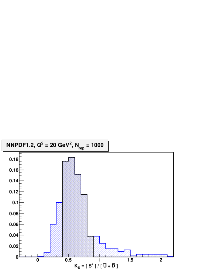
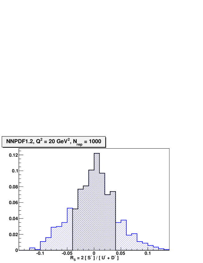
The value and uncertainty on these quantities can be determined from the NNPDF1.2 set by performing averages over replica PDFs [21], which for and will not necessarily coincide with the ratio of average PDFs, because Eqs. (17-18) are not linear in the PDFs. In fact, because the denominator in Eq. (17) can assume rather small values, we expect that the distribution of values of the total strange fraction can be rather asymmetric and non-gaussian. The probability distribution of at GeV2 is shown in Fig. 13, and turns out to be indeed quite far from gaussian. Therefore, we compute the one- uncertainty as a central 68% confidence integral, namely requiring the two outer tails of the probability distribution (lighter blue region in Fig. 13) to each correspond to 16% probability, with the central value still given by the average. The result we thus obtain for the expected and its uncertainty are shown in Table 9, along with the results found using other parton sets. The median of the probability distribution is equal to , significantly different from the average because of the asymmetry. The NNPDF1.2 uncertainty is much larger than that found in other fits, for the reasons discussed above. Note that, however, all values are essentially consistent with the simple assumption used in older parton fits.
| Analysis | Reference | [GeV2] | ||
|---|---|---|---|---|
| NNPDF1.2 | This work | |||
| MSTW08 | [15] | 1 | ||
| CTEQ6.5s | [13] | 1.69 | ||
| CTEQ6.1s | [11] | 1.69 | ||
| AKP08 | [14] | 20 | ||
| NuTeV07 | [10] | 16 | ||
| BPPZ03 | [42] | 20 |
In the case of the strange momentum asymmetry Eq. (18) the denominator is fixed by knowledge of the valence content of the nucleon, which is known quite accurately: hence we expect the uncertainty to be symmetric and dominated by uncertainty of the numerator. Indeed, the probability distribution for , shown in Fig. 14, turns out to be approximately gaussian so that the uncertainty computed from the central 68% confidence essentially coincides with the standard deviation of the distribution, while central value and uncertainty for are essentially proportional to those of the strangeness asymmetry . This latter quantity has been determined by various groups, at various scales: several of these results are collected in Table 10 and compared to our own. Results are given both at the scale at which they were determined, and then also when evolved to a common scale, exploiting the fact that at NLO (though not at NNLO [43]) evolves multiplicatively. In this case, too, the NNPDF1.2 uncertainty is much larger than that obtained in other fits: while for all other groups there is an indication that a positive value of is favored (all results being nevertheless compatible with zero), this indication looses its significance in our analysis due to the very large uncertainty.
In the next section we will see that, surprisingly, even with such large uncertainties it is possible to exploit our determination of and for a determination of electroweak parameters. In view of this, it is useful to also study possible sources of systematic uncertainty on these quantities. Possible significant sources of systematics are the following:
-
•
Heavy quark mass effects. The treatment of heavy quark mass effects entails various ambiguities related to the prescription used to deal with subleading terms [33]. In our case, a further source of systematics is due to the fact that the charm quark mass is treated approximately, using the I-ZM-VFN scheme as discussed in Sect. 3.3, and then only for dimuon data. The corresponding uncertainty is conservatively estimated by repeating the fit in a pure ZM-VFN scheme.
- •
-
•
Higher order QCD corrections. These are very conservatively estimated by repeating the fit at LO.
| (mean) | ||
|---|---|---|
| Reference | ||
| ZM-VFN | ||
| Nuclear - dFS03 | ||
| Nuclear - HKN07 | ||
| LO | ||
| No strange SR |
The results from and obtained in each of these cases are compared in Table 11 to the reference NNPDF1.2 result, all at the scale GeV2. It is apparent that the effect of any of these systematics is rather moderate, even if very conservatively estimated. In the same table we also show the result of a fit in which the sum rule Eq. (9) is not imposed: even in this case the result changes very little.
Estimating the effect of the systematics from the sum in quadrature of the shift of central values due to the four central rows of Table 11 we get, at GeV2
| (19) | |||||
| (20) |
The systematics on is thus negligible, and mostly due to nuclear effects. The systematics on is not quite negligible, and almost entirely due to the treatment of the heavy quark mass: this is an aspect of our analysis which could be improved in the future within a more accurate treatment of quark mass effects.
4.5 Comparison with experimental data
The results obtained from a NLO computation of the dimuon cross section from the reference set of NNPDF1.2 parton distributions with replicas are compared in Fig. 15 to the NuTeV experimental data. The agreement is clearly excellent in all bins except for the lowest values (bottom left plot), where the approximate treatment of the quark mass leads to a deterioration in quality of the fit.
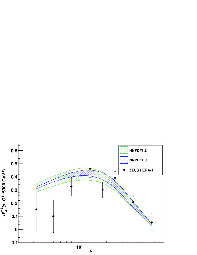
In Ref. [26], an extraction of the interference parity–violating structure function evolved to a common scale GeV2 was also presented. This extraction is based on data already included in our fit, so these data do not provide any extra information. However, it is interesting to compare directly to it, because this structure function is directly sensitive to the flavour and valence/sea decomposition of PDFs (specifically to strangeness), which is difficult to probe directly (see e.g. Ref. [21], appendix A.2). Because the contribution of to the total reduced cross–section is small and only relevant in a limited region of phase space, the agreement between data and theory for this quantity could in principle be poor without this being significantly reflected in the quality of the global fit.
| NNPDF 1.0 | TeV | 8.49 0.18 | 5.81 0.13 | 1.36 0.02 |
| TeV | 11.83 0.26 | 8.41 0.20 | 1.95 0.04 | |
| NNPDF 1.1 | TeV | 8.52 0.33 | 5.79 0.28 | 1.36 0.04 |
| TeV | 11.86 0.46 | 8.38 0.39 | 1.95 0.06 | |
| NNPDF 1.2 | TeV | 8.61 0.25 | 5.85 0.15 | 1.37 0.03 |
| TeV | 11.99 0.34 | 8.47 0.21 | 1.97 0.04 |
A comparison of these data with the NLO prediction obtained using the NNPDF1.0 and NNPDF1.2 parton sets is shown in Fig. 16, and shows good agreement: for NNPDF1.2, and for NNPDF1.0, comparable to the value for other data in the valence region (despite the fact that for the NNPDF1.0 fit neither the data of Ref. [26] nor dimuon data were used). The widening of the uncertainty band when going from NNPDF1.0 to NNPDF1.2 is a consequence of the sensitivity of this structure function to valence combinations, and strangeness in particular: very precise measurements of it could greatly improve flavour separation of PDFs.
A detailed study of the phenomenological implications of our reassessment of the strangeness uncertainty for LHC observables is beyond the scope of this work. However, in Table 12 we collect the total cross section for and production computed at NLO with MCFM [44, 45, 46, 47]: results obtained with the NNPDF1.2 and NNPDF1.1 parton sets are compared to those found using NNPDF1.0. already discussed in Ref. [21]. Because of the increased uncertainty on the strange distribution, the uncertainty in the cross section is larger in NNPDF1.1 and NNPDF1.2, though less so in NNPDF1.2 due to the constraint from dimuon data.
5 Precision determination of electroweak parameters
Neutrino DIS data, and especially dimuon data, can be used to perform direct measurements of electroweak parameters [48, 49]. However the potential precision of these measurements can be spoiled by PDF uncertainties. Indeed, we have seen in Sect. 4 that the uncertainties we obtain on the strange distributions are quite large, typically larger by almost one order of magnitude than those found in previous global fits.
The CKM matrix elements control the strength of the coupling of various partons to neutrinos according to Eqs. (11,12). In spite of the large PDF uncertainties in the strange sector, we shall provide here the most precise direct determination up to date of the CKM matrix element within a single experiment. We will also provide a determination of with an accuracy consistent with previous results from neutrino data. These remarkable results are possible because PDF uncertainties are free from parametrization bias, thus they may be disentangled from the uncertainty on the physical parameters.
We will then turn to a study of the impact of PDF uncertainties on the extraction of the electroweak mixing angle from the Paschos-Wolfenstein ratio: we will show that once PDF uncertainties are properly taken into account, the NuTeV measurement of this ratio [1] is in full agreement with the standard model prediction.
5.1 Determination of and .
Since the pioneering CDHS studies [41], neutrino DIS has been used as a means to directly determine CKM matrix elements: the parton–model expressions for the neutrino and anti-neutrino dimuon production Eqs. (11,12) provide two equations which relate two experimentally measurable cross sections to the two unknowns and .
However, these equations also contain as unknowns the second moments of the light quark PDFs (the total cross section is proportional to the second moment of the PDF). The standard lore [41, 31, 24] is then that if one assumes that , the linear combination only depends on the and the and valence components, which are well measured by other experiments, so it can be used to determine . On the other hand, the orthogonal combination depends on the ratio, but also on Eq. (17), and thus it can only be used to determine the combination . Indeed, the PDG [24] quotes a value of obtained from the average neutrino dimuon experiments as the best current direct determination. Only the bound at 90% confidence level [31] was quoted in previous PDG [50] editions, but this is now superseded by a direct determination from decays (for a recent update, see Ref. [51]). Of course, the values obtained from the current global CKM fits [52, 53, 24] are much more precise than these direct determinations (see Table 14 below).
In the NNPDF1.2 reference fit, , , and are each fixed to the current PDG value [24], obtained from the global CKM unitarity fit. We now show that, thanks to the fact that we are free of bias related to the parametrization of strangeness, we can extract both and from the fit. In order to do this, we perform a scan over the values of and used in the fit, holding fixed, but relaxing the unitarity constraint (in practice, because of its smallness, the precise value chosen for is inconsequential). The best–fit value and uncertainty for the CKM parameters are then determined in the standard way by maximum likelihood from the profile.
The determined from a set of data points fluctuates, with a standard deviation equal to . In order to determine the profile as the underlying parameters are varied, these fluctuations must be kept under control. Within our Monte Carlo approach, this could be done by using the same set of data replicas each time the is recomputed with different values of the underlying parameters. This might however bias the result in a random way depending on the particular set of replicas which has been chosen in the first place. We prefer thus to vary randomly the set of replicas which is used for different parameter values: fluctuations are then kept under control by using a sufficiently large set of replicas, given the fluctuation of the computed from a replica average has a standard deviation equal to . Because only dimuon data are sensitive to the CKM matrix elements, we can determine their values from the dependence of the of the fit to these data only, rather than for that of the fit to the global dataset. Because we have (see Tab. 1) dimuon data points, a set of replicas is sufficient to guarantee that point-by-point fluctuations are smaller than .
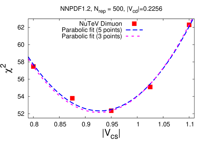
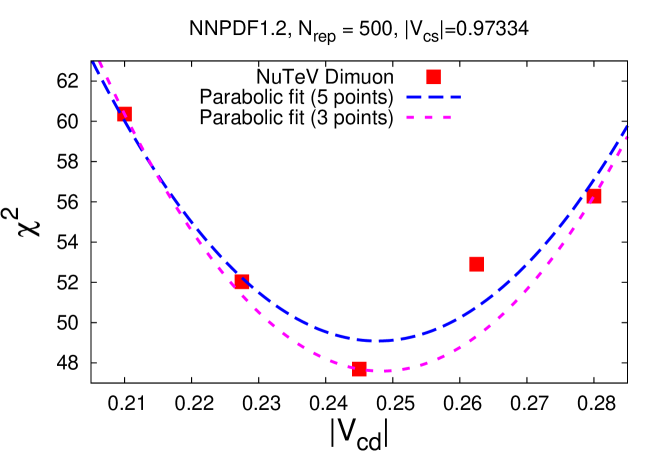
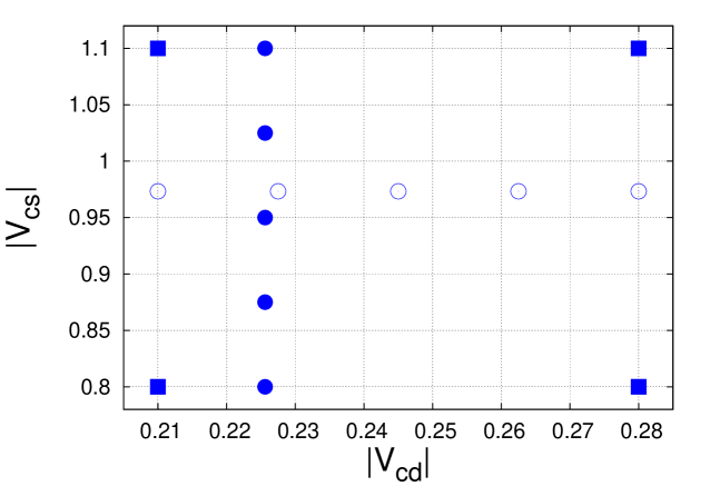
First, we vary independently each of the two CKM matrix elements, keeping the other fixed at its central value in the CKM unitarity fit. The profile is computed for five equally spaced values of the parameter which is being varied. The values have been chosen on the basis of a preliminary exploration of the space of parameters based on fits with a small number of replicas; they are displayed in Fig. 19. The ensuing profile is displayed in Fig. 17 for and in Fig. 18 for . We observe well-defined minima in both cases. A parabolic fit leads to
| (21) | |||||
| (22) |
where the one- uncertainty is obtained from the condition . The fit is quite stable upon the choice of different subsets of the five available points: if it is repeated by only retaining the central and two outer points neither the central values nor the uncertainties Eqs. (21-22) vary significantly. This confirms that the number of replicas used to compute the is sufficiently large for the result not to be biased by statistical fluctuations. Both fits are shown in Figs. 17-18.
This shows that either CKM matrix element can be determined from our data, with comparable uncertainty, by taking the other fixed. We can thus perform a simultaneous determination of both these CKM matrix elements. In order to improve the accuracy of this determination, we compute the at four more points in the (, ) plane, denoted by squares in Fig. 19. The in these additional points is computed from a smaller set of replicas. The result of the combined fit is then
| (23) | |||||
| (24) |
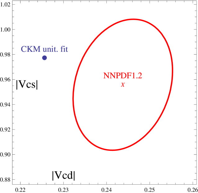
The uncertainties turn out to be almost identical to the diagonal uncertainties, and the correlation coefficient is relatively small , reflected in a moderate shift in central values in comparison to the separate fits Eqs. (21-22). The location of the best-fit point and one- () ellipse in the (, ) plane for the best-fit paraboloid is shown in Fig. 20.
| Statistical | ||
|---|---|---|
| Mass effects | ||
| Higher order QCD | ||
| Nuclear corrections | ||
| Total systematic uncertainty | ||
| Total uncertainty |
This determination Eq. (24) is affected by the same systematics that we examined in Sect. 4.3, namely, higher order QCD corrections, treatment of heavy quark effects and modeling of nuclear corrections. In order to assess their impact in the CKM element determination, we have repeated the determination of each of the two parameters as the other is kept fixed, Eqs. (21-22), by recomputing the for a smaller set of replicas along the points denoted as circles in Fig. 19, with each of these three effects varied in turn as we did in Sect. 4.3. We then take the shift in central value as an estimate of the corresponding uncertainty. The results are summarized in Table 13. Putting everything together, we find
| (25) | |||||
| (26) |
In Table 14 we compare our final results Eqs. (25-26) with the best CKM unitarity fit results and with other direct determinations. Our determination of is consistent with other direct determinations, and of comparable accuracy, though one should bear in mind that previous determinations from dimuon data were based on fits with a fixed functional form, and thus subject to potentially large systematics bias. Our determination of is rather more accurate that any other direct determination from dimuon data, more accurate than any single direct determination, and of comparable accuracy to the PDF average of determinations from decays.
| Analysis | Description | Reference | |
|---|---|---|---|
| NNPDF1.2 | Direct determination from global PDF analysis | This work | |
| CDHS | LO determination from | [41] | (90% C.L.) |
| CCFR | NLO determination from | [28, 31] | (90% C.L.) |
| PDG08 | Averages of determinations from decays | [24] | |
| Hocker | Averages of determinations from | [54] | |
| DELPHI | Direct measurement from decays | [55] | |
| PDG08 | CKM unitarity fit | [24] |
5.2 PDF corrections to the Paschos-Wolfenstein ratio
The successful determination of the CKM matrix elements which control charged current scattering suggests that we might use our parton set for a reliable reassessment of the determination of the coupling which controls neutral current neutrino DIS. As is well known [56], this coupling depends on the electroweak mixing angle, which can thus be extracted from its experimental measurement. Specifically, in the parton model one has
| (27) | |||||
where is the electroweak mixing angle, is the strange valence momentum fraction Eq. (16), , and the valence momentum fractions of other quark flavors, and .
The recent experimental determination [1]
| (28) |
is obtained using Eq. (27) under the assumption that for an isoscalar nucleon target -===, so the term in square brackets in Eq. (27) vanishes. Of course, the NuTeV iron target is not exactly isoscalar; however, the corresponding correction can be computed [1] with small uncertainty [2]. The result Eq. (28) disagrees at the three- level with the value determined in global precision electroweak fits, such as [57, 58]
| (29) |
Possible explanations for this include nuclear effects, electroweak corrections, QCD corrections, and physics beyond the standard model [2] (see e.g. [59] for an updated list of references). However, one may also[2] question the validity of the assumption of the vanishing of the contribution in square brackets in Eq. (27). The possibility that even for an isoscalar target due to isospin violation induced by QED evolution effects was discussed in Ref. [60]: it could easily explain about a third of the observed discrepancy.
In our fit, isospin symmetry is assumed, and furthermore . We are then left with the correction
| (30) |
with defined in Eq. (18). Using the value of Eq. (20), obtained at the typical scale GeV2 of the NuTeV data (and whose scale dependence is very small anyway [43]) we obtain
| (31) |
where the theoretical uncertainty comes from the effects discussed above in Sect. 4.3, and it is not to be confused with the experimental systematics in the NuTeV measurement Eq. (28).
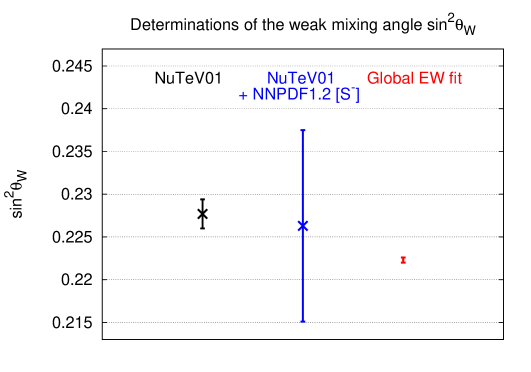
Even neglecting these theoretical uncertainties (which we estimated very conservatively), the additional PDF uncertainty due to strangeness alone is thus about twice the observed discrepancy in . We must conclude therefore that the apparent inconsistency between the NuTeV measurement and the global electroweak fit disappears once the uncertainty on the strange distribution is properly taken into account. Applying the correction Eq. (31) the NuTeV result becomes
| (32) |
We recommend that the corrected result Eq. (32) be used, for instance in global electroweak fits. This corrected result is compared graphically in Fig. 21 to the original NuTeV result Eq. (28) and the result from the global electroweak fit Eq. (29).
6 Conclusions and outlook
We have presented an upgrade of the NNPDF1.0 parton set, which now includes an independent parametrization for the strange distributions, and the inclusion of dimuon data which constrain them. Besides being an intermediate step towards a fully global fit including hadronic data, our results are interesting as a test of the NNPDF methodology, as a state-of-the art determination of the strange PDFs, and as a determination of electroweak parameters.
We have shown that the NNPDF approach has no difficulty in dealing with situations where experimental information is scarce and only provides loose constraints on the form of parton distributions. Within our approach, this does not require the introduction of theoretical assumptions or constraints in order to obtain stable results. We can thus provide reliable estimates of uncertainties, free of bias induced by theoretical assumptions.
We have obtained a determination of the strange momentum fraction and of the strangeness valence component, which, though in agreement with previous determinations, turn out to be affected by uncertainties which are sizably larger than those found by other groups.
Nevertheless, we have shown that, with the uncertainty on the strange PDF carefully estimated, the dimuon data can be used to provide a good determination of the CKM matrix elements and . In particular, our determination of is the most accurate ever obtained from neutrino deep-inelastic scattering data, and it is also more accurate than any individual direct determination from decays. We have also shown that once PDF uncertainties are estimated reliably, the value of the electroweak mixing angle extracted from NuTeV inclusive data is in agreement with standard model expectations.
The main defect of our results is that they are still based on an approximate treatment of the charm mass. Within the context of the present work, the only significant implication of this is a slight increase in the systematic uncertainty on our determination of . However, this also entails a further small but non-negligible systematic uncertainty in our determination of PDFs [21].
It will be interesting to study the implications for LHC observables of this reassessment of the uncertainty on the strange distribution. The NNPDF1.2 release is available from the webpage of the NNPDF Collaboration http://sophia.ecm.ub.es/nnpdf/.
Acknowledgments
This work was partly supported by grants
PRIN-2006 (Italy),
MEC FIS2004-05639-C02-01
(Spain) and by the European network HEPTOOLS under contract
MRTN-CT-2006-035505. L.D.D. is funded by an STFC Advanced Fellowship and
M.U. by a SUPA graduate studentship.
We acknowledge discussions with S. Alekhin, P. Nadolsky, P. Nason and
A. Vicini.
We are especially grateful to D. Mason for providing
us with the NuTeV data and acceptances, to F. Olness for information
on NLO acceptances, to R. Sassot and R. Petti for
providing us with their nuclear PDF sets and to A. Tapper and
K. Nagano
for help with the HERA-II data. J.R. acknowledges the hospitality
of the CERN TH Division where part of this work was completed.
Appendix A Kernels for Physical Observables
In this appendix we expand the physical observables for dimuon production in the evolution basis of the PDFs, and derive expressions for the kernels, in the same way and using the same notation as in Appendix A of Ref. [21]. All convolutions may be performed either in the ZM-VFNS or in the I-ZM-VFN scheme, as discussed in Sect. 3.3.
The cross-section for charm production in neutrino scattering off an isoscalar nucleon is given by Eq. (1), which we write as
| (33) |
where
| (34) |
Taking into account a possible non-isoscalar component of the nuclear target by defining , in the quark model we have
| (35) | |||
| (36) |
where all explicit dependence on and has been dropped. In terms of the PDF evolution eigenstates we then have
| (37) |
where the +(-) sign corresponds to neutrino (anti-neutrino) scattering, and the CKM factors are
| (38) |
Unitarity of the CKM matrix is imposed setting ; in the CKM determination in Sec. 5.2 it is however left unconstrained. Below threshold , so .
In perturbative QCD the charm production neutrino structure functions thus take the form
| (39) | |||
| (40) |
where and is the number of active flavours. We can thus write the charm production neutrino cross-sections as
| (41) |
where in Mellin space the kernels are
| (42) | |||||
| (43) | |||||
| (44) | |||||
| (45) | |||||
| (46) |
Below the threshold the singlet kernels simplify to
| (47) | |||||
| (48) | |||||
| (49) |
References
- [1] NuTeV, G.P. Zeller et al., Phys. Rev. Lett. 88 (2002) 091802.
- [2] S. Davidson et al., JHEP 02 (2002) 037.
- [3] W.K. Tung et al., JHEP 02 (2007) 053.
- [4] A.D. Martin et al., Phys. Lett. B652 (2007) 292.
- [5] V. Barone, C. Pascaud and F. Zomer, Eur. Phys. J. C12 (2000) 243.
- [6] NuTeV, M. Tzanov et al., Phys. Rev. D74 (2006) 012008.
- [7] CHORUS, G. Onengut et al., Phys. Lett. B632 (2006) 65.
- [8] NuTeV, M. Goncharov et al., Phys. Rev. D64 (2001) 112006.
- [9] CHORUS, A. Kayis-Topaksu et al., Nucl. Phys. B798 (2008) 1.
- [10] D. Mason et al., Phys. Rev. Lett. 99 (2007) 192001.
- [11] F. Olness et al., Eur. Phys. J. C40 (2005) 145.
- [12] S. Kretzer et al., Phys. Rev. Lett. 93 (2004) 041802.
- [13] H.L. Lai et al., JHEP 04 (2007) 089.
- [14] S. Alekhin, S. Kulagin and R. Petti, (2008), arXiv:0812.4448.
- [15] A.D. Martin et al., (2009), arXiv:0901.0002.
- [16] G. Watt et al., (2008), arXiv:0806.4890.
- [17] P.M. Nadolsky et al., (2008), arXiv:0802.0007.
- [18] S. Forte et al., JHEP 05 (2002) 062.
- [19] NNPDF, L. Del Debbio et al., JHEP 03 (2005) 080.
- [20] NNPDF, L. Del Debbio et al., JHEP 03 (2007) 039.
- [21] NNPDF, R.D. Ball et al., Nucl. Phys. B809 (2009) 1.
- [22] M. Dittmar et al., (2009), arXiv:0901.2504.
- [23] NNPDF, J. Rojo et al., (2008), arXiv:0811.2288.
- [24] Particle Data Group, C. Amsler et al., Phys. Lett. B667 (2008) 1.
- [25] D.A. Mason, FERMILAB-THESIS-2006-01.
- [26] ZEUS, S. Chekanov et al., (2009), arXiv:0901.2385.
- [27] ZEUS, S. Chekanov et al., (2008), arXiv:0812.4620.
- [28] CCFR, A.O. Bazarko et al., Z. Phys. C65 (1995) 189.
- [29] D. Mason, Private communication, 2009.
- [30] F. Olness, Private communication, 2009.
- [31] T. Bolton, (1997), hep-ex/9708014.
- [32] J. Pumplin, H.L. Lai and W.K. Tung, Phys. Rev. D75 (2007) 054029.
- [33] R.S. Thorne and W.K. Tung, (2008), arXiv:0809.0714.
- [34] P.M. Nadolsky and W.K. Tung, (2009), arXiv:0903.2667.
- [35] D. de Florian and R. Sassot, Phys. Rev. D69 (2004) 074028.
- [36] M. Hirai, S. Kumano and T.H. Nagai, Phys. Rev. C76 (2007) 065207.
- [37] S.A. Kulagin and R. Petti, Phys. Rev. D76 (2007) 094023.
- [38] K.J. Eskola, H. Paukkunen and C.A. Salgado, (2009), arXiv:0902.4154.
- [39] H. Honkanen, S. Liuti, J. Carnahan, Y. Loitiere and P. R. Reynolds, Phys. Rev. D79 (2009) 034022.
- [40] D. de Florian, R. Sassot, M. Stratmann and W. Vogelsang, Phys. Rev Lett. 101 (2008) 072001.
- [41] H. Abramowicz et al., Z. Phys. C15 (1982) 19.
- [42] V. Barone et al., JHEP 01 (2006) 006.
- [43] S. Catani et al., Phys. Rev. Lett. 93 (2004) 152003.
- [44] J.M. Campbell and R.K. Ellis, Phys. Rev. D62 (2000) 114012.
- [45] J. Campbell and R.K. Ellis, Phys. Rev. D65 (2002) 113007.
- [46] J. Campbell, R.K. Ellis and F. Tramontano, Phys. Rev. D70 (2004) 094012.
- [47] MCFM, http://mcfm.fnal.gov.
- [48] J. Conrad, M. Shaevitz and T. Bolton, Rev. Mod. Phys. 70 (1998) 1341.
- [49] M.L. Mangano et al., (2001), hep-ph/0105155.
- [50] Particle Data Group, D.E. Groom et al., Eur. Phys. J. C15 (2000) 1.
- [51] S. Narison, Phys. Lett. B668 (2008) 308.
- [52] UTFit, http://www.utfit.org.
- [53] HEPDATA, http://ckmfitter.in2p3.fr/.
- [54] A. Hocker et al., Eur. Phys. J. C21 (2001) 225.
- [55] DELPHI, P. Abreu et al., Phys. Lett. B439 (1998) 209.
- [56] E.A. Paschos and L. Wolfenstein, Phys. Rev. D7 (1973) 91.
- [57] H. Flacher et al., (2008), arXiv:0811.0009.
- [58] S. Heinemeyer, W. Hollik and G. Weiglein, Phys. Rept. 425 (2006) 265.
- [59] J.T. Londergan, Eur. Phys. J. A32 (2007) 415.
- [60] A.D. Martin et al., Eur. Phys. J. C39 (2005) 155.