One-dimensional stability of parallel shock
layers in isentropic magnetohydrodynamics

Abstract

Extending investigations of Barker, Humpherys, Lafitte, Rudd, and Zumbrun for compressible gas dynamics and Freistühler and Trakhinin for compressible magnetohydrodynamics, we study by a combination of asymptotic ODE estimates and numerical Evans function computations the one-dimensional stability of parallel isentropic magnetohydrodynamic shock layers over the full range of physical parameters (shock amplitude, strength of imposed magnetic field, viscosity, magnetic permeability, and electrical resistivity) for a $\gamma$-law gas with $\gamma\in[1,3]$. Other $\gamma$-values may be treated similarly, but were not checked numerically. Depending on magnetic field strength, these shocks may be of fast Lax, intermediate (overcompressive), or slow Lax type; however, the shock layer is independent of magnetic field, consisting of a purely gas-dynamical profile. In each case, our results indicate stability. Interesting features of the analysis are the need to renormalize the Evans function in order to pass continuously across parameter values where the shock changes type or toward the large-amplitude limit at frequency $\lambda=0$ and the systematic use of winding number computations on Riemann surfaces.

1 Introduction

In this paper, continuing investigations of [4, 27, 13], we study by a combination of asymptotic ODE estimates and numerical Evans function computations the one-dimensional stability of parallel isentropic magnetohydrodynamic (MHD) shock layers over a full range of physical parameters, including arbitrarily large shock amplitude and strength of imposed magnetic field, for a $\gamma$-law gas with $\gamma\in[1,3]$, with our main emphasis on the case of an ideal monatomic or diatomic gas. The restriction to $\gamma\in[1,3]$ is an arbitrary one coming from the choice of parameters on which the numerical study is carried out; stability for other $\gamma$ can be easily checked as well. (Note that our analytical results are for any $\gamma\geq 1$.) In each case, we obtain results indicative of stability. Recall that Evans stability, defined in terms of the Evans function associated with the linearized operator about the wave, by the “Lyapunov-type” results of [38, 39, 51, 52, 23, 24, 46], implies linear and nonlinear stability for all except the measure-zero set of parameters on which the characteristic speeds of the endstates coincide with the shock speed or each other.

Parallel shocks may be of fast Lax, intermediate (overcompressive), or slow Lax type depending on magnetic field strength; however, the shock layer is independent of magnetic field, consisting of a purely gas-dynamical profile. Thus, the study of their stability is both a natural next step to and an interesting generalization of the investigations of stability of gas-dynamical shocks in [27]. See also the investigations of stability of fast parallel Lax shocks in certain parameter regimes in [13] using energy methods, and of general fast Lax shocks in the small-magnetic field limit in [20, 19] using Evans function techniques.

1.1 Equations

In Lagrangian coordinates, the equations for compressible isentropic MHD in one dimension take the form

$$\left\{\begin{array}[]{l}v_{t}-u_{1x}=0,\\ u_{1t}+(p+(1/2\mu_{0})(B_{2}^{2}+B_{3}^{2}))_{x}=(((2\mu+\eta)/v)u_{1x})_{x},\\ u_{2t}-((1/\mu_{0})B_{1}^{*}B_{2})_{x}=((\mu/v)u_{2x})_{x},\\ u_{3t}-((1/\mu_{0})B_{1}^{*}B_{3})_{x}=((\mu/v)u_{3x})_{x},\\ (vB_{2})_{t}-(B_{1}^{*}u_{2})_{x}=((1/\sigma\mu_{0}v)B_{2x})_{x},\\ (vB_{3})_{t}-(B_{1}^{*}u_{3})_{x}=((1/\sigma\mu_{0}v)B_{3x})_{x},\\ \end{array}\right.$$ (1.1)

where $v$ denotes specific volume, $u=(u_{1},u_{2},u_{3})$ velocity, $p=p(v)$ pressure, $B=(B_{1}^{*},B_{2},B_{3})$ magnetic induction, $B_{1}^{*}$ constant, and $\mu>0$ and $\eta>0$ the two coefficients of viscosity, $\mu_{0}>0$ the magnetic permeability, and $\sigma>0$ the electrical resistivity; see [3, 10, 33, 35] for further discussion.

We restrict to an ideal isentropic polytropic gas, in which case the pressure function takes form

$$p(v)=av^{-\gamma}$$ (1.2)

where $a>0$ and $\gamma>1$ are constants that characterize the gas. In our numerical investigations, we shall focus mainly on the most common cases of a monatomic gas, $\gamma=5/3$, and a diatomic gas, $\gamma=7/5$; more generally, we investigate all $\gamma\in[1,3]$. With brief exceptions (e.g., Section 4.4), we take

$$\eta=-2\mu/3,$$ (1.3)

as typically prescribed for (nonmagnetic) gas dynamics [5].

Here, we are allowing $u$ and $B$ to vary in full three-dimensional space, but restricting spatial dependence to a single direction $e_{1}$ measured by $x$. That is, we consider planar solutions, or three-dimensional solutions with one-dimensional dependence on spatial variables. Note that the divergence-free condition ${\rm div}_{x}B\equiv 0$ of full MHD reduces in the planar case to our assumption that $B_{1}\equiv\text{\rm constant}=B_{1}^{*}$. In the simplest, parallel case

$$B_{2}=B_{3}\equiv 0;\,u_{2}=u_{3}\equiv 0,$$ (1.4)

equations (1.1) reduce to the one-dimensional isentropic compressible Navier–Stokes equations

$$\left\{\begin{array}[]{l}v_{t}-u_{1x}=0,\\ u_{1t}+p_{x}=(((2\mu+\eta)/v)u_{1x})_{x}.\\ \end{array}\right.$$ (1.5)

In the remainder of the paper, we study traveling-wave solutions in this special parallel case and their stability with respect to general (not necessarily parallel) planar perturbations.

1.2 Viscous shock profiles

A viscous shock profile of (1.1) is an asymptotically-constant traveling-wave solution

$$(v,u,B)(x,t) =(\hat{v},\hat{u},\hat{B})(x-st),\quad\lim_{z\to\pm\infty}=(v_{\pm},u_{\pm},B_{\pm}).$$ (1.6)

In the parallel case, these are of the simple form

$$(\hat{v},\hat{u},\hat{B})(x-st)=(\hat{v},\hat{u}_{1},0,0,B_{1}^{*},0,0)(x-st),$$

where $(\hat{v},\hat{u}_{1})$ is a gas-dynamical shock profile satisfying the traveling-wave ODE

$$\left\{\begin{array}[]{l}-sv_{x}-u_{1x}=0,\\ -su_{1x}+p_{x}=(((2\mu+\eta)/v)u_{1x})_{x}.\\ \end{array}\right.$$ (1.7)

1.3 Rescaled equations

By a preliminary rescaling in $x$, $t$, we may arrange without loss of generality $\mu=1$. Following the approach of [27, 29, 28], we now rescale

$$(v,u_{1},u_{2},u_{3},\mu_{0},x,t,B)\to\Big{(}\frac{v}{\varepsilon},-\frac{u_{1}}{\varepsilon s},\frac{u_{2}}{\varepsilon},\frac{u_{3}}{\varepsilon},\varepsilon\mu_{0},-\varepsilon s(x-st),\varepsilon s^{2}t,\frac{B}{s}\Big{)}$$

holding $\mu$, $\sigma$ fixed, where $\varepsilon:=v_{-}$, transforming (1.1) to the form

$$\left\{\begin{aligned} v_{t}+v_{x}-u_{1x}&=0\\ u_{1t}+u_{1x}+\left(av^{-\gamma}+\left(\frac{1}{2\mu_{0}}\right)\left(B_{2}^{2}+B_{3}^{2}\right)\right)_{x}&=(2\mu+\eta)\left(\frac{u_{1x}}{v}\right)_{x}\\ u_{2t}+u_{2x}-\left(\frac{1}{\mu_{0}}B_{1}^{*}B_{2}\right)_{x}&=\ \mu\left(\frac{u_{2x}}{v}\right)_{x}\\ u_{3t}+u_{3x}-\left(\frac{1}{\mu_{0}}B_{1}^{*}B_{3}\right)_{x}&=\mu\left(\frac{u_{3x}}{v}\right)_{x}\\ \left(vB_{2}\right)_{t}+\left(vB_{2}\right)_{x}-\left(B_{1}^{*}u_{2}\right)_{x}&=\left(\left(\frac{1}{\sigma\mu_{0}v}\right)B_{2x}\right)_{x}\\ \left(vB_{3}\right)_{t}+\left(vB_{3}\right)_{x}-\left(B_{1}^{*}u_{3}\right)_{x}&=\left(\left(\frac{1}{\sigma\mu_{0}v}\right)B_{3x}\right)_{x}\end{aligned}\right.$$ (1.8)

where $p(v)=a_{0}v^{-\gamma}$ and $a=a_{0}\varepsilon^{-\gamma-1}s^{-2}$.

By this step, we reduce without loss of generality to the case of a shock profile with speed $s=-1$, left endstate

$$(v,u_{1},u_{2},u_{3},B_{1},B_{2},B_{3})_{-}=(1,0,0,0,B_{1}^{*},0,0),$$ (1.9)

and right endstate

$$(v,u_{1},u_{2},u_{3},B_{1},B_{2},B_{3})_{+}=(v_{+},v_{+}-1,0,0,B_{1}^{*},0,0),$$ (1.10)

satisfying the profile ODE

$$(2\mu+\eta)v^{\prime}=H(v,v_{+}):=v(v-1+a(v^{-\gamma}-1))$$ (1.11)

(obtained by integrating (1.7) and substituting the first equation into the second) where $1=v_{-}\geq v_{+}>0$ and (setting $v^{\prime}=0$ at $v=v_{+}$ and solving)

$$a=-\frac{v_{+}-1}{v_{+}^{-\gamma}-1}=v_{+}^{\gamma}\frac{1-v_{+}}{1-v_{+}^{\gamma}}.$$ (1.12)

See [4, 27] for further details.

Proposition 1.1 ([4]).

For each $\gamma\geq 1$, $0<v_{+}\leq 1-\varepsilon$, $\varepsilon>0$, (1.11) has a unique (up to translation) monotone decreasing solution $\hat{v}$ decaying to its endstates with a uniform exponential rate, independent of $v_{+}$, $\gamma$. In particular, for $0<v_{+}\leq\frac{1}{12}$ and $\hat{v}(0):=v_{+}+\frac{1}{12}$,

$$|{\hat{v}}(x)-v_{+}| \leq\Big{(}\frac{1}{12}\Big{)}e^{-\frac{3x}{4}}\quad x\geq 0,$$ (1.13a)

$$|{\hat{v}}(x)-v_{-}| \leq\Big{(}\frac{1}{4}\Big{)}e^{\frac{x+12}{2}}\quad x\leq 0.$$ (1.13b)

Corollary 1.2.

Initializing $\hat{v}(0):=v_{+}+\frac{1}{12}$ as in Proposition 1.1, $\hat{v}$ converges uniformly as $v_{+}\to 0$ to a translate $\hat{v}_{0}$ of $\frac{1-\tanh\big{(}\frac{x}{2(2\mu+\eta)}\big{)}}{2}$.

Proof.

By (1.12), $a\sim v_{+}^{\gamma}\to 0$ as $v_{+}\to 0$, whence the result follows on any bounded set $|x|\leq L$ by continuous dependence, taking the limit as $a\to 0$ in (1.11) to obtain a limiting flow of $v^{\prime}=\frac{v(1-v)}{2\mu+\eta}$. Taking now $L\to\infty$, the result follows for $|x|\geq M$ by $v_{+}\to 0$ and $|\hat{v}-v_{+}|\leq Ce^{-\theta M}$; see (1.13a)–(1.13b). ∎

1.4 Families of shock profiles

At this point, we have reduced our study of parallel shock stability, for a fixed gas constant $\gamma$, to consideration of a one-parameter family of profiles indexed by the right endstate $1\geq v_{+}>0$ and a four-parameter family of equations (1.8) indexed (through (1.12)) by $v_{+}$ and the three remaining physical parameters

$$\mu_{0}>0,\,\sigma>0,\,B_{1}^{*}\geq 0,$$ (1.14)

where we have taken $B_{1}^{*}$ without loss of generality to be nonnegative by use of the symmetry under $B\to-B$ of (1.1). Here, the small-amplitude limit corresponds to $v_{+}\to v_{-}=1$ and the large-amplitude limit to $v_{+}\to 0$, where in this scaling the amplitude is given by $|v_{-}-v_{+}|$.

A straightforward computation shows that the characteristics of the first-order hyperbolic system obtained by neglecting second-derivative terms in (1.8) at the endstates $v_{\pm}$ have values

$$(1\pm c(v)),1,1,\Big{(}1\pm\frac{B_{1}^{*}}{\sqrt{\mu_{0}v_{\pm}}}\Big{)},$$ (1.15)

where $c(v):=\sqrt{-p^{\prime}(v)}=\sqrt{\gamma av^{-\gamma-1}}$ is the gas-dynamical sound speed, satisfying $c_{+}>1>c_{-}$. Thus, the shock is a Lax $1$-shock for $0\leq B_{1}^{*}<\sqrt{\mu_{0}v_{+}}$, meaning that it has six positive characteristics at $v_{-}$ and one at $v_{+}$; an intermediate doubly overcompressive shock for $\sqrt{\mu_{0}v_{+}}<B_{1}^{*}<\sqrt{\mu_{0}}$, meaning that it has six positive characteristics at $v_{-}$ and three at $v_{+}$; and a Lax $3$-shock for $\sqrt{\mu_{0}}<B_{1}^{*}$, meaning that it has $4$ positive characteristics at $v_{-}$ and three at $v_{+}$.

For Lax $1$- and $3$-shocks, the profile (1.6) is generically (and always for $1$-shocks) unique up to translation as a traveling-wave solution of the full equations connecting endstates (1.9) and (1.10), i.e., even among possibly nonparallel solutions. That is, it lies generically within a one-parameter family $\{\hat{U}^{\xi}\}=\{(\hat{v},\hat{u}_{1},\hat{u}_{2},\hat{u}_{3},\hat{B}_{2},\hat{B}_{3})^{\xi}\}$ of viscous shock profiles, $\xi\in\mathbb{R}$, with $\hat{U}^{\xi}(x):=\hat{U}(x-\xi)$. For overcompressive shocks, it lies generically within a three-parameter family $\{(\hat{v},\hat{u}_{1},\hat{u}_{2},\hat{u}_{3},\hat{B}_{2},\hat{B}_{3})^{\xi}\}$ of viscous profiles and their translates, $\xi\in\mathbb{R}^{3}$, of which it is the unique parallel solution up to translation [38]. For further discussion of hyperbolic shock type and its relation to existence of viscous profiles, see, e.g., [37, 55, 50, 51, 38].

1.5 Evans, spectral, and nonlinear stability

Following [55, 38, 51], define spectral stability as nonexistence of nonstable eigenvalues $\Re\lambda\geq 0$ of the linearized operator about the wave, other than at $\lambda=0$ (where there is always an eigenvalue, due to translational invariance of the underlying equations). A slightly stronger condition is Evans stability, which for Lax or overcompressive shocks may be defined [55, 38, 28] as nonvanishing for all $\Re\lambda\geq 0$ of the Evans function associated with the integrated eigenvalue equation about the wave. See [1, 16, 50, 51, 38] for a general definition of the Evans function associated with a system of ordinary differential equations; for a definition in the present context, see Section 2. Recall that zeros of the Evans function (either integrated or nonintegrated) agree with eigenvalues of the linearized operator about the wave on $\{\Re\lambda\geq 0\}\setminus\{0\}$, so that Evans stability implies spectral stability.

The following “Lyapunov-type” result of Raoofi [45], specialized to our case, states that, for generic parameter values, Evans stability implies nonlinear orbital stability, regardless of the type of the shock; see also [39, 51, 24, 46].

Proposition 1.3 ([45]).

Let $\hat{U}:=(\hat{v},\hat{u}_{1},\hat{u}_{2},\hat{u}_{3},\hat{B}_{2},\hat{B}_{3})$ be a parallel viscous shock profile of (1.1)–(1.2) connecting endstates (1.9)–(1.10), with characteristics (1.15) distinct and nonzero, that is Evans stable. Then, for any solution $\tilde{U}:=(\tilde{v},\tilde{u}_{1},\tilde{u}_{2},\tilde{u}_{3},\tilde{B}_{2},\tilde{B}_{3})$ of (1.1) with $L^{1}\cap H^{3}$ initial difference and $L^{1}$-first moment $E_{0}:=\|\tilde{U}(\cdot,0)-\hat{U}\|_{L^{1}\cap H^{3}}$ and $E_{1}:=\||x|\,|\tilde{U}(\cdot,0)-\hat{U}|\|_{L^{1}}$ sufficiently small and some uniform $C>0$, $\tilde{U}$ exists for all $t\geq 0$, with

$$\|\tilde{U}(\cdot,t)-\hat{U}(\cdot-st)\|_{L^{1}\cap H^{3}} \leq CE_{0}\quad\hbox{\rm(stability)}.$$ (1.16)

Moreover, there exist $\alpha(t)$, $\alpha_{\infty}$ such that

$$\|\tilde{U}(\cdot,t)-\hat{U}^{\alpha(t)}(\cdot-st))\|_{L^{p}} \leq CE_{0}(1+t)^{-(1/2)(1-1/p)},$$ (1.17)

and

$$|\alpha(t)-\alpha_{\infty}|,\,(1+t)^{1/2}|\dot{\alpha}(t)|\leq C(\varepsilon)\max\{E_{0},E_{1}\}(1+t)^{-1/2+\varepsilon},$$ (1.18)

for all $1\leq p\leq\infty$, $\varepsilon>0$ arbitrary  (phase-asymptotic orbital stability).

Finally, recalling that Evans stability for Lax shocks is equivalent to the three conditions of spectral stability, transversality of the traveling wave as a connecting orbit of (1.11), and inviscid stability of the shock while Evans stability for overcompressive shocks is equivalent to spectral stability, transversality, and an “inviscid stability”-like low-frequency stability condition generalizing the Lopatinski condition of the Lax case [55, 38, 51], we obtain the following partial converse allowing us to make stability conclusions from spectral information alone.

Proposition 1.4.

A parallel viscous shock profile of (1.1)–(1.2), (1.9)–(1.10), that is a Lax $1$-shock and spectrally stable is also Evans stable (hence, for generic parameters, nonlinearly orbitally stable). A parallel viscous shock profile that is an intermediate (overcompressive) shock, spectrally stable and low-frequency stable is Evans stable. A parallel viscous shock profile that is a Lax $3$-shock, spectrally stable, and transverse is Evans stable. For $\mu=1$ and $B_{1}^{*}\geq\max\left\{\sqrt{\frac{\gamma\mu_{0}}{2}},\sqrt{\frac{\gamma}{2\sigma}}\,\right\}+\sqrt{\mu_{0}}$, Lax $3$-shocks are transverse. For parallel viscous shocks of any type, spectral stability implies Evans (and nonlinear) stability on a generic set of parameters.

Proof.

Lax $1$-shocks and intermediate-shocks, as extreme shocks (i.e., all characteristics entering the shock from the $-\infty$ side), are always transversal [38]. One-dimensional inviscid stability of either Lax $1$- or $3$-shocks follows by a straightforward calculation using decoupling of the linearized equations into $(v,u_{1})$ and $(u_{2},B_{2})$ and $(u_{3},B_{3})$ systems [6, 49, 13]. Transversality for large $B_{1}^{*}$ is shown in Proposition B.3. Finally, both transversality (in the Lax $3$-shock case) and (in the overcompressive case) low-frequency stability conditions can be expressed as nonvanishing of functions that are analytic in the model parameters, hence either vanish everywhere or on a measure zero set. It may be shown that these are both nonvanishing for sufficiently weak profiles $|1-v_{+}|$ small, hence they are generically nonvanishing. From these facts, the result follows. ∎

Remark 1.5.

Our numerical results indicate Evans stability for all parameters, which implies in passing uniform transversality of $3$- and overcompressive-shock profiles and low-frequency stability of overcompressive profiles. Transversality is a minimal condition for orbital stability, being needed even to guarantee existence of the smooth manifold $\hat{U}^{\alpha}$ under discussion [38]. As discussed above, it is not implied by spectral stability alone.

1.6 The reduced linearized eigenvalue equations

Linearizing (1.8) about a parallel shock profile $(\hat{v},\hat{u}_{1},0,0,B_{1}^{*},0,0)$, we obtain a decoupled system

$$\left\{\begin{aligned} v_{t}+v_{x}-u_{1x}&=0\\ u_{1t}+u_{1x}-a\gamma\left(\hat{v}^{-\gamma-1}v\right)_{x}&=(2\mu+\eta)\left(\frac{u_{1x}}{\hat{v}}+\frac{\hat{u}_{1x}}{\hat{v}^{2}}v\right)_{x}\\ u_{2t}+u_{2x}-\frac{1}{\mu_{0}}(B_{1}^{*}B_{2})_{x}&=\ \mu\left(\frac{u_{2x}}{\hat{v}}\right)_{x}\\ u_{3t}+u_{3x}-\frac{1}{\mu_{0}}(B_{1}^{*}B_{3})_{x}&=\ \mu\left(\frac{u_{3x}}{\hat{v}}\right)_{x}\\ \left(\hat{v}B_{2}\right)_{t}+\left(\hat{v}B_{2}\right)_{x}-(B_{1}^{*}u_{2})_{x}&=\left(\left(\frac{1}{\sigma\mu_{0}}\right)\frac{B_{2x}}{\hat{v}}\right)_{x}\\ \left(\hat{v}B_{3}\right)_{t}+\left(\hat{v}B_{3}\right)_{x}-(B_{1}^{*}u_{3})_{x}&=\left(\left(\frac{1}{\sigma\mu_{0}}\right)\frac{B_{3x}}{\hat{v}}\right)_{x},\end{aligned}\right.$$ (1.19)

consisting of the linearized isentropic gas dynamic equations in $(v,u_{1})$ about profile $(\hat{v},\hat{u}_{1})$, and two copies of an equation in variables $(u_{j},\hat{v}B_{j})$, $j=2,3$.

Introducing integrated variables $V:=\int v$, $U:=\int u_{1}$ and $w_{j}:=\int u_{j}$, $\alpha_{j}:=\int\hat{v}B_{j}$, $j=2,3$, we find that the integrated linearized eigenvalue equations decouple into the integrated linearized eigenvalue equations for gas dynamics in variables $(V,U)$ and two copies of

$$\left\{\begin{aligned} \lambda w+w^{\prime}-\frac{B_{1}^{*}\alpha^{\prime}}{\mu_{0}\hat{v}}&=\mu\frac{w^{\prime\prime}}{\hat{v}}\\ \lambda\alpha+\alpha^{\prime}-B_{1}^{*}w^{\prime}&=\frac{1}{\sigma\mu_{0}\hat{v}}\left(\frac{\alpha^{\prime}}{\hat{v}}\right)^{\prime}\end{aligned}\right.$$ (1.20)

in variables $(w_{j},\alpha_{j})$, $j=2,3$.

As noted in [55, 38, 28], spectral stability is unaffected by the change to integrated variables. Thus, spectral stability of parallel MHD shocks, decouples into the conditions of spectral stability of the associated gas-dynamical shock as a solution of the isentropic Navier–Stokes equations (1.5), and spectral stability of system (1.20). Assuming stability of the gas-dynamical shock (as has been verified in great generality in [27, 29]), spectral stability of parallel MHD shocks thus reduces to the study of the reduced eigenvalue problem (1.20), into which the shock structure enters only through density profile $\hat{v}$. Likewise, the Evans function associated with the full system (1.19) decouples into the product of the Evans function for the gas-dyamical eigenvalue equations and the Evans function for the reduced eigenvalue problem (1.20). Thus, assuming stability of the associated gas-dynamical shock, Evans stability of parallel MHD shocks reduces to Evans stability of (1.20).

Remark 1.6.

The change to integrated coordinates removes two additional zeros of the Evans function for the reduced equations (1.20) that would otherwise occur at the origin in the overcompressive case, making possible a unified study across different parameter values/shock types.

1.7 Analytical stability results

1.7.1 The case of infinite resistivity/permeability

We start with the observation that, by a straightforward energy estimate, parallel shocks are unconditionally stable in transverse modes $(\tilde{u},\tilde{B})$ in the formal limit as either electrical resistivity $\sigma$ or magnetic permeability $\mu_{0}$ go to infinity, for quite general equations of state. This is suggestive, perhaps, of a general trend toward stability.

Theorem 1.7.

In the degenerate case $\mu_{0}=\infty$ or $\sigma=\infty$, parallel MHD shocks are transversal, Lopatinski stable (resp. low-frequency stable), and spectrally stable with respect to transverse modes $(\tilde{u},\tilde{B})$, for all physical parameter values, hence are Evans (and thus nonlinearly) stable whenever the associated gas-dynamical shock is Evans stable.

Proof.

By Proposition 1.4, Lopatinski stability holds for Lax-type shocks, and transversality holds for Lax $1$-shocks and overcompressive shocks. Noting that the (decoupled) transverse part of linearized traveling-wave ODE for $\sigma=\infty$ or $\mu_{0}=\infty$ reduces to $(d-1)$ copies of the same scalar equation, and recalling that transversality/Lopatinski stability hold always for the decoupled gas-dynamical part [27], we readily verify low-frequency stability in the overcompressive case and transversality in the Lax $3$-shock case as well. Thus, we need only verify transverse spectral stability, or nonexistence of decaying solutions of (1.20).

For $\sigma=\infty$, we may rewrite (1.20) in symmetric form as

$$\mu_{0}\hat{v}\lambda w+\mu_{0}\hat{v}w^{\prime}-B_{1}^{*}\alpha^{\prime} =\mu\mu_{0}w^{\prime\prime},$$ (1.21)

$$\lambda\alpha+\alpha^{\prime}-B_{1}^{*}w^{\prime} =0.$$

Taking the real part of the complex $L^{2}$-inner product of $w$ against the first equation and $\alpha$ against the second equation and summing gives

$$\Re\lambda(\int(\hat{v}\mu_{0}|w|^{2}+|\alpha|^{2})=-\int\mu\mu_{0}|w^{\prime}|^{2}+\int\hat{v}_{x}|w|^{2}<0,$$

a contradiction for $\Re\lambda\geq 0$ and $w$ not identically zero. If $w\equiv 0$ on the other hand, we have a constant-coefficient equation for $\alpha$, which is therefore stable. The $\mu_{0}=\infty$ case goes similarly; see Appendix B.2. ∎

Notably, this includes all three cases: fast Lax, overcompressive, and slow Lax type shock. Further, the same proof yields the result for the more general class of equations of state $p(\cdot)$ satisfying $\frac{p(v_{+})-p(v_{-})}{v_{+}-v_{-}}<0$, so that $\hat{v}_{x}<0$ for $s<0$. With the analytical results of [27], we obtain in particular the following asymptotic results.

Corollary 1.8.

For $\sigma=\infty$ or $\mu_{0}=\infty$, parallel isentropic MHD shocks with ideal gas equation of state, whether Lax or overcompressive type, are linearly and nonlinearly stable in the small- and large-amplitude limits $v_{+}\to 1$ and $v_{+}\to 0$, for all physical parameter values.

1.7.2 Bounds on the unstable spectrum

By a considerably more sophisticated energy estimate, we can bound the size of unstable eigenvalues uniformly in $1\geq v_{+}>0$ and the gas constant $\gamma\geq 1$ to a ball of radius depending on $\sigma$, $\mu_{0}$, $B_{1}^{*}$, a crucial step in studying the limit $v_{+}\to 0$.

Theorem 1.9.

Nonstable eigenvalues $\Re\lambda\geq 0$ of (1.20) are confined for $0<v_{+}\leq 1$ to the region

$$\Re\lambda+|\Im\lambda|<\frac{1}{2}\max\Big{\{}\frac{1}{\mu},\mu_{0}\sigma\Big{\}}+(B_{1}^{*})^{2}\sqrt{\dfrac{\sigma}{\mu\mu_{0}}}.$$ (1.22)

Proof.

See Appendix B. ∎

1.7.3 Asymptotic Evans function analysis

Denoting by $D(\lambda)$ the “reduced” Evans function (defined Section 2) associated with the reduced eigenvalue equations (1.20), we introduce the pair of renormalizations

$$\check{D}(\lambda) :=\frac{\Big{(}(1-B_{1}^{*}/\sqrt{\mu_{0}})^{2}+4\lambda(\mu/2+1/2\sigma\mu_{0})\Big{)}^{1/4}}{\Big{(}(1-B_{1}^{*}/\sqrt{\mu_{0}})^{2}+4(\mu/2+1/2\sigma\mu_{0})\Big{)}^{1/4}}\frac{\Big{(}v_{+}/4+\lambda\Big{)}^{1/4}}{\Big{(}v_{+}/4+1\Big{)}^{1/4}}$$ (1.23)

$$\quad\times\frac{\Big{(}(1-B_{1}^{*}/\sqrt{\mu_{0}v_{+}})^{2}+4\lambda(\mu/2v_{+}+1/2\sigma\mu_{0}v_{+}^{2})\Big{)}^{1/4}}{\Big{(}(1-B_{1}^{*}/\sqrt{\mu_{0}v_{+}})^{2}+4(\mu/2v_{+}+1/2\sigma\mu_{0}v_{+}^{2})\Big{)}^{1/4}}D(\lambda)$$

and

$$\hat{D}(\lambda) :=\frac{\Big{(}(1-B_{1}^{*}/\sqrt{\mu_{0}})^{2}+4\lambda(\mu/2+1/2\sigma\mu_{0})\Big{)}^{1/4}}{\Big{(}(1-B_{1}^{*}/\sqrt{\mu_{0}})^{2}+4(\mu/2+1/2\sigma\mu_{0})\Big{)}^{1/4}}D(\lambda).$$ (1.24)

Intermediate behavior.

Theorem 1.10.

On $\Re\lambda\geq 0$, the reduced Evans function $D$ is analytic in $\lambda$ and continuous in all parameters except at $v_{+}=0$ and $B_{1}=\sqrt{\mu_{0}v_{\pm}}$, at which points it exhibits algebraic singularities (blow-up) at $\lambda=0$. The renormalized Evans functions $\check{D}$ and $\hat{D}$ are analytic in $\lambda$ and continuous in all parameters except at $(\lambda,v_{+})=(0,0)$.

Proof.

Immediate from Propositions 2.13 and 3.6. ∎

The small-amplitude limit.

Proposition 1.11 ([31, 44]).

For $\sigma>0$, $\mu_{0}>0$, $B_{1}^{*}>0$ bounded, and $B_{1}^{*}$ bounded away from $\sqrt{\mu_{0}}$, parallel shocks are Evans stable in both full and reduced sense in the small-amplitude limit $v_{+}\to 1$. Moreover, $D$ converges uniformly on compact subsets of $\{\Re\lambda\geq 0\}$ as $v_{+}\to 1$ to a nonzero real constant.

Proof.

For $|v_{-}-v_{+}|=|1-v_{+}|$ sufficiently small and $B_{1}^{*}$ bounded away from $\sqrt{\mu_{0}}$, the associated profile must be a Lax $1$- or $3$-shock, whence stability follows by the small-amplitude results obtained by energy estimates in [31] or by asymptotic Evans function techniques in [44]. Convergence on compact sets follows by the argument of Proposition 4.9, [29], which likewise uses techniques from [44]. ∎

The large-amplitude limit.

Theorem 1.12.

For $\sigma$, $\mu_{0}$ and $B_{1}^{*}$ bounded, the reduced Evans function $D(\lambda)$ converges uniformly on compact subsets of $\{\Re\lambda\geq 0\}\setminus\{0\}$ in the large-amplitude limit $v_{+}\to 0$ to a limiting Evans function $D^{0}(\lambda)$ obtained by substituting $\hat{v}_{0}$ for $\hat{v}$ in (1.20), $\hat{v}_{0}$ as in Proposition 1.2; see Definition 3.4 for a precise definition. Likewise, $\check{D}$ and $\hat{D}$ converge to

$$\check{D}^{0}(\lambda):=\frac{\Big{(}1-B_{1}^{*}/\sqrt{\mu_{0}})^{2}+4\lambda(\mu/2+1/2\sigma\mu_{0})\Big{)}^{1/4}}{\Big{(}1-B_{1}^{*}/\sqrt{\mu_{0}})^{2}+4(\mu/2+1/2\sigma\mu_{0})\Big{)}^{1/4}}\lambda^{1/2}D^{0}(\lambda)$$ (1.25)

and

$$\hat{D}^{0}(\lambda):=\frac{\Big{(}(1-B_{1}^{*}/\sqrt{\mu_{0}})^{2}+4\lambda(\mu/2+1/2\sigma\mu_{0})\Big{)}^{1/4}}{\Big{(}(1-B_{1}^{*}/\sqrt{\mu_{0}})^{2}+4(\mu/2+1/2\sigma\mu_{0})\Big{)}^{1/4}}D^{0}(\lambda),$$ (1.26)

each continuous on $\Re\lambda\geq 0$. Moreover, for $B_{1}^{*}<\sqrt{\mu_{0}}$, nonvanishing of $\check{D}^{0}$ on $\{\Re\lambda>0\}$ is necessary and nonvanishing of $\check{D}^{0}$ on $\{\Re\lambda\geq 0\}$ is sufficient for reduced Evans stability (i.e., nonvanishing of $\check{D}$, $D$ on $\{\Re\lambda>0\}$ for $v_{+}>0$ sufficiently small. For $B_{1}^{*}>\sqrt{\mu_{0}}$, nonvanishing of $\hat{D}^{0}$ on $\{\Re\lambda>0\}$ is necessary and nonvanishing of $\hat{D}^{0}$ on $\{\Re\lambda\geq 0\}$ together with a certain sign condition on $\hat{D}(0)$ is sufficient for reduced Evans stability for $v_{+}>0$ sufficiently small. This sign condition is implied in particular by nonvanishing of $\hat{D}(0)$ on the range

$$\sqrt{\mu_{0}}\leq B_{1}^{*}\leq\sqrt{\mu_{0}}+\max\Big{\{}\sqrt{\frac{\mu_{0}}{2}},\sqrt{\frac{1}{2\sigma}}\,\Big{\}}.$$ (1.27)

Proof.

Convergence follows by Proposition 3.6; for stability criteria, see Section 3.5. ∎

Remark 1.13.

The theoretically cumbersome condition (1.27) is in practice no restriction, since we check in any case the stronger condition of nonvanishing of $\hat{D}$ for $\Re\lambda\geq 0$ on the entire range $\sqrt{\mu_{0}}\leq B_{1}^{*}\leq\sqrt{\mu_{0}}+\max\Big{\{}\sqrt{\frac{\mu_{0}}{2}},\sqrt{\frac{1}{2\sigma}}\,\Big{\}}$.

Remark 1.14.

Recall [27] that the associated gas-dynamical shock has already been shown to be Evans stable for $v_{+}>0$ sufficiently small. Thus, not only reduced Evans stability, but full Evans stability, is implied for $v_{+}>0$ sufficiently small by stability of the limiting function $\check{D}^{0}$ (resp. $\hat{D}^{0}$).

Large- and small-parameter limits.

Theorem 1.15.

For $\sigma$, $\mu_{0}$ bounded and bounded from zero, and $v_{+}$ bounded from zero, parallel shocks are reduced Evans stable in the limit as $B_{1}^{*}\to\infty$ or $B_{1}^{*}\to 0$. For $\lambda$ bounded and $\Re\lambda\geq 0$, the Evans function converges as $B_{1}^{*}\to\infty$ to a constant.

Theorem 1.16.

For $B_{1}^{*}$ bounded, and $v_{+}$ bounded from zero, parallel shocks are reduced Evans stable in the limit as $\sigma\to 0$ with $\mu_{0}$ bounded, $\mu_{0}\to 0$ with $\sigma$ bounded. In each case, the Evans function converges uniformly to zero on compact subsets of $\{\Re\lambda\geq 0\}$, with $C^{-1}\sqrt{\sigma}\leq|D^{\sigma}(\lambda)|\leq C\sqrt{\sigma}$ for $C\sigma\leq|\lambda|\leq C$ and $C^{-1}\sqrt{\mu_{0}}\leq|D^{\sigma}(\lambda)|\leq C\sqrt{\mu_{0}}$ for $C\mu_{0}\leq|\lambda|\leq C$.

Theorem 1.17.

For $B_{1}^{*}$ bounded, and $v_{+}$ and $\mu_{0}$ bounded from zero, parallel shocks are reduced Evans stable in the limit as $\sigma\mu_{0}\to\infty$. For $\lambda$ bounded and $\Re\lambda\geq 0$, the Evans function $D$, appropriately renormalized, converges as $\sigma\mu_{0}\to\infty$ to the Evans function $\hat{D}$ for (1.21); more precisely, $D\sim e^{c_{0}\sigma\mu_{0}+c_{1}+c_{2}\lambda}\hat{D}$ for $c_{j}$ constant.

Remark 1.18.

Except for certain “corner points” consisting of simultaneous limits of $B_{1}^{*}\to\infty$ together with $\sigma\to 0$, or $\sigma\mu_{0}\to\infty$ together with $v_{+}\to 0$ or $\mu_{0}\to 0$, our analytic results verify stability on all but a (large but) compact set of parameters. We conjecture that stability holds in these limits as well; this would be an interesting question for further investigation.

As pointed out in [29], the limit $v_{+}\to 0$ is connected with the isentropic approximation, and does not occur for full (nonisentropic) MHD for gas constant $\gamma>1$; thus, a somewhat more comprehensive analysis is possible in that case. Note that the reduced eigenvalue equations are identical in the nonisentropic case [13], except with $\hat{v}$ replaced by a full (nonisentropic) gas-dynamical profile, from which observation the reader may check that all of the analytical results of this paper goes through unchanged in the nonisentropic case, since the analysis depends only on $\hat{v}$, and this only through properties of monotone decrease, $|v_{x}|\leq C|v|$ (immediate for $v$ bounded from zero), and uniform exponential convergence as $x\to\pm\infty$, that are common to both the isentropic and nonisentropic ideal gas cases.

Discussion. Taken together, and along with the previous theoretical and numerical investigations of [27] on stability of gas-dynamical shocks, our asymptotic stability results reduce the study of stability of parallel MHD shocks, in accordance with the general philosophy set out in [27, 29, 28], mainly (i.e., with the exception of “corner points” discussed in Remark 1.18) to investigation of the continuous and numerically well-conditioned renormalized functions $\check{D}$ and $\hat{D}$ on a compact parameter-range suitable for discretization, together with investigation of the similarly well-conditioned limiting functions $\check{D}^{0}$ and $\hat{D}^{0}$. However, notice that the same results show that the unrenormalized Evans function $D$ blows up as $\lambda\to 0$, both in the large-amplitude limit $v_{+}\to 0$ and in the characteristic limits $B_{1}^{*}\to\sqrt{\mu_{0}v_{\pm}}$, hence is not suitable for numerical testing across the entire parameter range. Indeed, in practice these singularities dominate behavior even rather far from the actual blow-up points, making numerical investigation infeasibly expensive if renormalization is not carried out, even for intermediate values of parameters/frequencies. This is a substantial difference between the current and previous analyses, and represents the main new difficulty that we have overcome in the present work.

1.8 Numerical stability results

For a given amplitude, the above analytical results truncate the computational domain to a compact set, thus allowing for a comprehensive numerical Evans function study patterned after [27, 29], which yields Evans stability in the intermediate parameter range. We then demonstrate Evans stability in the large-amplitude limit by (i) verifying convergence to the limiting Evans functions given in Theorem 1.12 (i.e., checking that convergence has occurred to desired tolerance at the limits of values $v_{+}$, $\lambda$ considered), and (ii) verifying nonvanishing on $\Re\lambda\geq 0$ of the limiting functions $\hat{D}^{0}$, $\check{D}^{0}$. These computational results, together with the analytical results in Section 1.7, give unconditional stability for all values except for cases where two or more parameters blow up simultaneously as described in Remark 1.18. The numerical computations were performed by the authors’ STABLAB package, which is written in MATLAB, and has been used successfully for several systems [4, 27, 29, 11, 26, 28].

When compared to the numerical study for isentropic Navier-Stokes [4, 27], this present system is better conditioned, yet much more computationally taxing since there are more free parameters to cover, i.e., $(\gamma,v_{+},B^{*}_{1},\mu_{0},\sigma)$; the isentropic model by contrast has only two parameters $(\gamma,v_{+})$. Since each dimension adds, roughly, an order of magnitude to the runtime, we upgraded our STABLAB package to allow for parallel computation via MATLAB’s parallel computing toolbox. In our main study, we computed along $30,\!870$ semi-circular contours corresponding to the parameter values

$$(\gamma,v_{+},B^{*}_{1},\mu_{0},\sigma)\in[1.0,3.0]\times[10^{-5},0.8]\times[0.2,3.8]\times[0.2,3.8]\times[0.2,3.8].$$

In every case, the winding number was zero, thus demonstrating Evans stability; see Section 5 for more details.

We also carried out a number of small studies to illustrate our analytical work in the limiting fixed-amplitude cases. These are briefly described below and are also given more detail in Section 5.

$\begin{array}[]{lr}\includegraphics[width=213.39566pt]{figures/vplimit}&\includegraphics[width=213.39566pt]{figures/vplimit_zoom}\end{array}$

Figure 1: Renormalized Evans function output for semi-circular contour of radius $4.5$ (left) as the amplitude varies. Parameters are $B^{*}_{1}=2$, $\mu_{0}=1$, $\sigma=1$, $\gamma=5/3$, with $v_{+}=10^{-1},10^{-1.5},10^{-2},10^{-2.5},10^{-3},10^{-3.5},10^{-4},10^{-4.5},10^{-5},10^{-5.5},10^{-6}$. Note the striking concentric structure of the contours, which converge to the outer contour in the large-amplitude limit (i.e., $v_{+}\rightarrow 0$) and to a non-zero constant in the small-amplitude limit (i.e., $v_{+}\rightarrow 1$), indicating stability for all shock strengths since the winding numbers throughout are all zero. The limiting contour given by $\hat{D}^{0}(\lambda)$ is also displayed, but is essentially identical to nearby contours. When the image is zoomed in near the origin (right), which is marked by a crosshair, we see that the curves are well behaved and distinct from the origin. Also clearly visible is the theoretically predicted square-root singularity at the origin of the limiting contour, as indicated by a right angle in the curve at the image of the origin on the real axis.

In Figure 1, we see the typical concentric structure as $v_{+}$ varies on $[0,1]$. Note that in the strong-shock limit, the output converges to the outer contour representing the Evans function output of the limiting system. In the small-amplitude limit, the system converges to a non-zero constant. Since the origin is outside of the contours, one can visually verify that the winding number is zero thus implying Evans stability, even in the strong-shock limit.

In Figure 2, we illustrate the convergence of the Evans function as $B^{*}_{1}\rightarrow\infty$. Note that the contours converge to zero, but they are stable for all finite values of $B^{*}_{1}$. Stability is proven analytically in Theorem 1.15 by a tracking argument. Prior to this computation, however, a significant effort was made to prove stability with energy estimates, but these efforts were in vain since the Evans function converges to zero as $B^{*}_{1}\rightarrow\infty$.

In Figure 3, we see the structure as $\mu_{0}\rightarrow 0$. Once normalized (right), we see that the structure is essentially unchanged despite a large variation in $\mu_{0}$; in particular, the shock layers are stable in the $\mu_{0}\rightarrow 0$ limit. This was proven analytically in Theorem 1.16.

Finally, in Figure 4, we see the behavior of the Evans function in the case that $r=\mu/(2\mu+\eta)\to\infty$. This is the opposite case of that considered in [13]. As we show in Proposition 4.3, this case can be computed by disengaging the shooting algorithm and just taking the determinant of initializing e-bases at $\pm\infty$. Notice that in this limit the shock layers are also stable.

$\begin{array}[]{cc}\includegraphics[width=213.39566pt]{figures/big_B}&\includegraphics[width=213.39566pt]{figures/big_B_zoom}\end{array}$

Figure 2: Evans function output for semi-circular contour of radius 5 (left) and a zoom-in of the same image near the origin (right). Parameters are $v_{+}=10^{-2}$, $\mu_{0}=1$, $\sigma=1$, $\gamma=5/3$, with $B^{*}_{1}=2,3.5,5,10,15,20,25,30,35,40$. Note that the contours converge to zero, which is marked by a cross hair, as $B^{*}_{1}\rightarrow\infty$.

$\begin{array}[]{cc}\includegraphics[width=213.39566pt]{figures/mu_small}&\includegraphics[width=213.39566pt]{figures/mu_small_normalized}\end{array}$

Figure 3: Evans function output for semi-circular contour of radius 5 (left) together with a renormalized version of the contours (right), where each contour is divided by its rightmost value, thus putting all contours through $z=1$ on the right side. Although these results are typical, the parameters in this example are $B^{*}_{1}=2$, $v_{+}=10^{-2}$, $\sigma=1$, $\gamma=5/3$, with $\mu_{0}=10^{-.5},10^{-1},10^{-1.5},10^{-2},10^{-2.5},10^{-3},10^{-3.5},10^{-4},10^{-4.5},10^{-5}$. Note that the renormalized contours are nearly identical. This provides a striking indication of stability for all values of $\mu_{0}$ in our range of consideration, and in particular for $\mu_{0}\rightarrow 0$.

$\begin{array}[]{cc}\includegraphics[width=213.39566pt]{figures/etaInfty}&\includegraphics[width=213.39566pt]{figures/etaInfty2}\end{array}$

Figure 4: Renormalized Evans function in the $r=\infty$ case. Parameters are $v_{+}=10^{-1}$, $10^{-2}$, $10^{-3}$, $10^{-4}$, $10^{-5}$, $10^{-6}$, $\mu_{0}=1$, $\sigma=1$, $\gamma=5/3$. We also have a semi-circular radius of $4.5$ with $B_{1}^{*}=2$ (left), and a semi-circular radius of $1$ with $B_{1}^{*}=0.5$ (right).

1.9 Discussion and open problems

Our numerical and analytical investigations suggest strongly (and in some cases rigorously prove) reduced Evans stability of parallel ideal isentropic MHD shock layers, independent of amplitude, viscosity and other transport parameters, or magnetic field, for gas constant $\gamma\in[1,3]$, indicating that they are stable whenever the associated gas-dynamical shock layer is stable. Together with previous investigations of [27] indicating unconditional stability of isentropic gas-dynamical shock layers for $\gamma\in[1,3]$, this suggests unconditional stability of parallel isentropic MHD shocks for gas constant $\gamma\in[1,3]$, the first such comprehensive result for shock layers in MHD.

It is remarkable that, despite the complexity of solution structure and shock types occurring as magnetic field and other parameters vary, we are able to carry out a uniform numerical Evans function analysis across almost (see Remark 1.18) the entire parameter range: a testimony to the power of the Evans function formulation. Interesting aspects of the present analysis beyond what has been done in the study of gas dynamical shocks in [27, 29] are the presence of branch singularities on certain parameter boundaries, necessitating renormalization of the Evans function to remove blow-up singularities, and the essential use of winding number computations on Riemann surfaces in order to establish stability in the large-amplitude limit. The latter possibility was suggested in [16] (see Remark 3, Section 2.1), but to our knowledge has not up to now been carried out.

We note that Freistühler and Trakhinin [13] have previously established spectral stability of parallel viscous MHD shocks using energy estimates in the regime

$$r:=\mu/(2\mu+\eta)\ll 1,$$

whenever $B_{1}^{*}<2\sqrt{\mu_{0}v_{-}}$ (translating their results to our setting $s=-1$), which includes all $1$- and intermediate-shocks, and some slow shocks ($B_{1}^{*}>\sqrt{\mu_{0}v_{-}}$). Recall that we have here followed the standard physical prescription $\eta=-2\mu/3$, so that $\mu/(2\mu+\eta)=3/4,$ outside the regime studied in [13]. Thus, the two analyses are complementary. It would be an interesting mathematical question to investigate stability for general ratios $\mu/(2\mu+\eta)$. See Section 4.4 for further discussion of this issue. Here we study only the limit $r\to\infty$ complementary to that studied by [13], the case $r=3/4$ suggested by nonmagnetic gas dynamics, and the remaining cases in the $r\to 0$ limit left open in [13]. Other $r$-values may be studied numerically, but were not checked.

Stability of general (not necessarily parallel) fast shocks in the small magnetic field limit has been established in [19] by convergence of the Evans function to the gas-dynamical limit, assuming that the limiting gas-dynamical shock is stable, as has been numerically verified for ideal gas dynamics in [27, 29, 28]. Stability of more general, non-gas-dynamical shocks with large magnetic field, is a very interesting open question. In particular, as noted in [48], one-dimensional instability, by stability index considerations, would for an ideal gas equation of state imply the interesting phenomenon of Hopf bifurcation to time-periodic, or “galloping” behavior at the transition to instability. For analyses of the related inviscid stability problem, see, e.g., [49, 6, 40] and references therein.

Another interesting direction for further investigation would be a corresponding comprehensive study of multi-dimensional stability of parallel MHD shock layers, as carried out for gas-dynamical shocks in [28]. As pointed out in [13], instability results of [6, 49] for the corresponding inviscid problem imply that parallel shock layers become multi-dimensionally unstable for large enough magnetic field, by the general result [56, 51] that inviscid stability is necessary for viscous stability, so that in multi-dimensions instability definitely occurs. The question in this case is whether viscous effects can hasten the onset of instability, that is, whether viscous instability can occur in the presence of inviscid stability.

2 The Evans function and its properties

We begin by constructing carefully the Evans function associated with reduced system (1.20), and recalling its basic properties for our later analysis.

2.1 The Evans system

The reduced eigenvalue equations (1.20) may be written as a first-order system

$$\begin{pmatrix}w\\ \mu w^{\prime}\\ \alpha\\ \frac{\alpha^{\prime}}{\sigma\mu_{0}\hat{v}}\end{pmatrix}^{\prime}=\begin{pmatrix}0&1/\mu&0&0\\ \lambda\hat{v}&\hat{v}/\mu&0&-\sigma B_{1}^{*}\hat{v}\\ 0&0&0&\sigma\mu_{0}\hat{v}\\ 0&-B_{1}^{*}\hat{v}/\mu&\lambda\hat{v}&\sigma\mu_{0}\hat{v}^{2}\end{pmatrix}\begin{pmatrix}w\\ \mu w^{\prime}\\ \alpha\\ \frac{\alpha^{\prime}}{\sigma\mu_{0}\hat{v}}\end{pmatrix},$$ (2.1)

or

$$W^{\prime}=A(x,\lambda)W,$$ (2.2)

indexed by the three parameters $B_{1}^{*}$, $\sigma$, and $\tilde{\mu}_{0}:=\sigma\mu_{0}$. Recall that we have already fixed $\mu=1$ and $(2\mu+\eta)=4/3$.

2.2 Limiting subspaces

Denote by

$$A_{\pm}(\lambda):=\lim_{x\to\pm\infty}A(x,\lambda)=\begin{pmatrix}0&1/\mu&0&0\\ \lambda v_{\pm}&v_{\pm}/\mu&0&-\sigma B_{1}^{*}v_{\pm}\\ 0&0&0&\sigma\mu_{0}v_{\pm}\\ 0&-B_{1}^{*}v_{\pm}/\mu&\lambda v_{\pm}&\sigma\mu_{0}v_{\pm}^{2}\end{pmatrix}$$ (2.3)

the limiting coefficient matrices associated with (2.1)-(2.2).

Lemma 2.1.

For $\Re\lambda\geq 0$, $\lambda\neq 0$, and $1\geq v_{+}>0$, each of $A_{\pm}$ has two eigenvalues with strictly positive real part and two eigenvalues with strictly negative real part, hence their stable and unstable subspaces $S_{\pm}$ and $U_{\pm}$ vary smoothly in all parameters and analytically in $\lambda$. For $v_{+}>0$ they extend continuously to $\lambda=0$, and analytically everywhere except at $B_{1}^{*}=\sqrt{\mu_{0}v_{\pm}}$, where they depend smoothly on $\sqrt{(1-B_{1}^{*}/\mu_{0}v_{\pm})^{2}+4\lambda c}$, $c:=\frac{1}{2}\Big{(}\frac{\mu}{v}+\frac{1}{\sigma\mu_{0}v^{2}}\Big{)}_{\pm}.$

Proof.

By standard hyperbolic–parabolic theory (e.g., Lemma 2.21, [51]), $A_{\pm}$ have no pure imaginary eigenvalues for $\Re\lambda\geq 0$, $\lambda\neq 0$, for any $v_{+}>0$ and parameter values $\sigma$, $\tilde{\mu}_{0}$, $B_{1}^{*}$, whence the numbers of stable (negative real part) and unstable (positive real part) eigenvalues are constant on this set. By homotopy taking $\lambda$ to positive real infinity, we find readily that there must be two of each.

Alternatively, we may see this directly by looking at the corresponding second-order symmetrizable hyperbolic–parabolic system

$$\lambda\begin{pmatrix}w\\ \alpha\end{pmatrix}+\begin{pmatrix}1&-B_{1}^{*}/\mu_{0}v_{\pm}\\ -B_{1}^{*}&1\end{pmatrix}\begin{pmatrix}w\\ \alpha\end{pmatrix}_{x}=\begin{pmatrix}\mu/v_{\pm}&0\\ 0&1/\sigma\mu_{0}v_{\pm}^{2}\end{pmatrix}\begin{pmatrix}w\\ \alpha\end{pmatrix}_{xx},$$

and applying the standard theory here, specifically, noting that eigenvalues consist of solutions $\mu$ of

$$\lambda\in\sigma\Big{(}-\mu\begin{pmatrix}1&-B_{1}^{*}/\mu_{0}v_{\pm}\\ -B_{1}^{*}&1\end{pmatrix}+\mu^{2}\begin{pmatrix}\mu/v_{\pm}&0\\ 0&1/\sigma\mu_{0}v_{\pm}^{2}\end{pmatrix}\Big{)},$$ (2.4)

so that $\mu=ik$ by a straightforward energy estimate yields $\Re\lambda\leq-\theta k^{2}$ for $\theta>0$.

Applying to reduced system (2.4) Lemma 6.1 [38] or Proposition 2.1, [55], we find further that, whenever the convection matrices

$$\beta_{\pm}:=\begin{pmatrix}1&-B_{1}^{*}/\mu_{0}v_{\pm}\\ -B_{1}^{*}&1\end{pmatrix}$$ (2.5)

are noncharacteristic in the sense that their eigenvalues $\alpha=1\pm\frac{B_{1}^{*}}{\sqrt{\mu_{0}v_{\pm}}}$ are nonzero, these subspaces extend analytically to $\lambda=0$.

Finally, we consider the degenerate case that $B_{1}^{*}=\sqrt{\mu_{0}v_{\pm}}$ and the convection matrix $\beta$ is characteristic. Considering (2.4) as determining $\lambda/\mu$ as a function of $\mu$ for $\mu$ small, we obtain, diagonalizing $B$ and applying standard matrix perturbation theory [34] that in the nonzero eigendirection $r_{j}$ of $\beta$, associated with eigenvalue $\beta_{j}\neq 0$, $\lambda/\mu\sim\beta_{j}$, and, inverting, we find that $\mu_{j}(\lambda)$ extends analytically to $\lambda=0$. In the zero eigendirection, on the other hand, associated with left and right eigenvectors $l=(1/2,1/2B_{1}^{*})^{T}$ and $r=(B,1)^{T}$, we find that

$$\lambda\sim-\mu(1-B_{1}^{*}/\sqrt{\mu_{0}v_{\pm}})+c\mu^{2}+\dots,$$

where

$$c=(l^{T}\beta r)_{\pm}=\frac{1}{2}\Big{(}\frac{\mu}{v}+\frac{1}{\sigma\mu_{0}v^{2}}\Big{)}_{\pm}\neq 0,$$

leading after inversion to the claimed square-root singularity. Likewise, the stable eigendirections of $A_{\pm}$ associated with $\mu$ vary continuously with $\lambda$, converging for $B_{1}^{*}=\sqrt{\mu_{0}v_{\pm}}$ and $\lambda=0$ to $(w,\alpha,w^{\prime},\alpha^{\prime})^{T}=\begin{pmatrix}r\\ 0\end{pmatrix},$ where $r$ is the zero eigendirection of $\beta$. This accounts for three eigenvalues $\mu$ lying near zero, bifurcating from the three-dimensional kernel of $A_{\pm}$ near a degenerate, characteristic, value of $B_{1}^{*}$. The fourth eigenvalue is far from zero and so varies analytically in all parameters about $\lambda=0$. ∎

Remark 2.2.

Remarkably, even though the shock changes type upon passage through the points $B_{1}^{*}=\sqrt{\mu_{0}v_{\pm}}$, the stable and unstable subspaces of $A_{\pm}$ vary continuously, with stable and unstable eigendirections coalescing in the characteristic mode.

2.3 Limiting eigenbases and Kato’s ODE

Denote by $\Pi_{+}$ and $\Pi_{-}$ the eigenprojections of $A_{+}$ onto its stable subspace and $A_{-}$ onto its unstable subspace, with $A_{\pm}$ defined as in (2.3). By Lemma 2.1, these are analytic in $\lambda$ for $\Re\lambda\geq 0$, $v_{+}>0$, except for square-root singularities at $\lambda=0$ for $B_{1}^{*}=\sqrt{\mu_{0}v_{\pm}}$. Introduce the complex ODE [34]

$$R^{\prime}=\Pi^{\prime}R,\quad R(\lambda_{0})=R_{0},$$ (2.6)

where ^′ denotes $d/d\lambda$, $\lambda_{0}$ is fixed with $\Re\lambda_{0}>0$, $\Pi=\Pi_{\pm}$, and $R$ is a $4\times 2$ complex matrix. By a partition of unity argument [34], there exists a choice of initializing matrices $R_{0}$ that is smooth in the suppressed parameters $v_{+}$, $B_{1}^{*}$, $\sigma$, and $\mu_{0}$, is full rank, and satisfies $\Pi(\lambda_{0})R_{0}=R_{0}$; that is, its columns are a basis for the stable (resp. unstable) subspace of $A_{+}$ (resp. $A_{-}$).

Lemma 2.3 ([34, 53]).

There exists a global solution $R$ of (2.6) on $\{\Re\lambda\geq 0\}$, analytic in $\lambda$ and smooth in parameters $v_{+}>0$, $B_{1}^{*}\geq 0$, $\sigma>0$, and $\mu_{0}>0$ except at the singular values $\lambda=0$, $B_{1}^{*}=\sqrt{\mu_{0}v_{\pm}}$, such that (i) ${\rm rank}R\equiv{\rm rank}R^{0}$, (ii) $\Pi R\equiv R$, and (iii) $\Pi R^{\prime}\equiv 0$.

Proof.

As a linear ODE with analytic coefficients, (2.6) possesses an analytic solution in a neighborhood of $\lambda_{0}$, that may be extended globally along any curve, whence, by the principle of analytic continuation, it possesses a global analytic solution on any simply connected domain containing $\lambda_{0}$ [34]. Property (i) follows likewise by the fact that $R$ satisfies a linear ODE. Differentiating the identity $\Pi^{2}=\Pi$ following [34] yields $\Pi\Pi^{\prime}+\Pi^{\prime}\Pi=\Pi^{\prime}$, whence, multiplying on the right by $\Pi$, we find the key property

$$\Pi\Pi^{\prime}\Pi=0.$$ (2.7)

From (2.7), we obtain

$$(\Pi R-R)^{\prime} =(\Pi^{\prime}R+\Pi R^{\prime}-R^{\prime})=\Pi^{\prime}R+(\Pi-I)\Pi^{\prime}R=\Pi\Pi^{\prime}R,$$

which, by $\Pi\Pi^{\prime}\Pi=0$ and $\Pi^{2}=\Pi$ gives

$$(\Pi R-R)^{\prime} =-\Pi\Pi^{\prime}(\Pi R-R),\quad(\Pi R-R)(\lambda_{0})=0,$$

from which (ii) follows by uniqueness of solutions of linear ODE. Expanding $\Pi R^{\prime}=\Pi\Pi^{\prime}R$ and using $\Pi R=R$ and $\Pi\Pi^{\prime}\Pi=0$, we obtain $\Pi R^{\prime}=\Pi\Pi^{\prime}\Pi R=0$, verifying (iii). ∎

Remark 2.4.

Property (iii) indicates that the Kato basis is an optimal choice in the sense that it involves minimal variation in $R$. It is useful also for computing the Kato basis in different ways [30, 7]; see Appendix C.

2.4 Characteristic values: the regularized Kato basis

We next investigate the behavior of the Kato basis near $\lambda=0$ and the degenerate points $B_{1}^{*}=\sqrt{\mu_{0}v_{\pm}}$ at which the reduced convection matrix $\beta_{\pm}$ of (2.5) becomes characteristic in a single eigendirection.

Example 2.5.

A model for this situation is the eigenvalue equation for a scalar convected heat equation $\lambda u+\eta u^{\prime}=u^{\prime\prime}$ with convection coefficient $\eta$ passing through zero. The coefficient matrix for the associated first-order system is

$$A:=\begin{pmatrix}0&1\\ \lambda&\eta\end{pmatrix}.$$ (2.8)

As computed in Appendix C, the stable eigenvector of $A$ determined by Kato’s ODE (2.6) is

$$R(\eta,\lambda):=\frac{(\eta^{2}/4+1)^{1/4}}{(\eta^{2}/4+\lambda)^{1/4}}\Big{(}1,-\eta/2-\sqrt{\eta^{2}/4+\lambda}\,\Big{)}^{T},$$ (2.9)

which, apart from the divergent factor $\frac{(\eta^{2}/4+1)^{1/4}}{(\eta^{2}/4+\lambda)^{1/4}}$, is a smooth function of $\sqrt{\eta^{2}/4+\lambda}$.

The computation of Example (2.5) indicates that the Kato basis blows up at $\lambda=0$ as $\big{(}(1-B_{1}^{*}/\sqrt{\mu_{0}v_{\pm}})^{2}+4\lambda\big{)}^{-1/4}$ as $B_{1}^{*}$ crosses characteristic points $\sqrt{\mu_{0}v_{\pm}}$ across which the shock changes type, hence does not give a choice that is continuous across the entire range of shock profiles. However, the same example shows that there is a different choice $(1,-\eta/2-\sqrt{\eta^{2}/4+\lambda}\,)^{T}$ that is continuous, possessing only a square-root singularity. We can effectively exchange one for another, by rescaling the Kato basis as we now describe.

Following [1, 16], associate with bases $R_{\pm}=(R_{1},R_{2})^{\pm}$ the wedge (i.e., exterior algebraic) product ${\cal R}_{\pm}:=(R_{1}\wedge R_{2})^{\pm}$.

Lemma 2.6.

The “regularized Kato products”

$$\tilde{\cal R}_{+}:=\frac{\Big{(}(1-B_{1}^{*}/\sqrt{\mu_{0}v_{+}})^{2}+4\lambda(\mu/2v_{+}+1/2\sigma\mu_{0}v_{+}^{2})\Big{)}^{1/4}}{\Big{(}(1-B_{1}^{*}/\sqrt{\mu_{0}v_{+}})^{2}+4(\mu/2v_{+}+1/2\sigma\mu_{0}v_{+}^{2})\Big{)}^{1/4}}(R_{1}^{+}\wedge R_{2}^{+})$$ (2.10)

and

$$\tilde{\cal R}_{-}:=\frac{\Big{(}(1-B_{1}^{*}/\sqrt{\mu_{0}})^{2}+4\lambda(\mu/2+1/2\sigma\mu_{0})\Big{)}^{1/4}}{\Big{(}(1-B_{1}^{*}/\sqrt{\mu_{0}})^{2}+4(\mu/2+1/2\sigma\mu_{0})\Big{)}^{1/4}}(R_{1}^{+}\wedge R_{2}^{+})$$ (2.11)

are analytic in $\lambda$ and smooth in remaining parameters on all of $\lambda\geq 0$, $v_{+}>0$, $B_{1}^{*}\geq 0$, $\sigma>0$, $\mu_{0}>0$ except the points $\lambda=0$, $B_{1}^{*}=\sqrt{\mu_{0}v_{\pm}}$, where they are continuous with a square-root singularity, depending smoothly on $\sqrt{(1-B_{1}^{*}/\sqrt{\mu_{0}v_{\pm}})^{2}+4\lambda}$. Moreover, they are bounded from zero (full rank) on the entire parameter range.

Proof.

A computation like that of Example 2.5 applied to system (2.3), replacing $\eta$ with the characteristic speed $1-B_{1}^{*}/\sqrt{\mu_{0}v_{\pm}}$ and introducing a diffusion coefficient $c_{\pm}=\frac{1}{2}\Big{(}\frac{\mu}{v}+\frac{1}{\sigma\mu_{0}v^{2}}\Big{)}_{\pm}$, i.e., considering

$$\lambda u+\eta u^{\prime}=cu^{\prime\prime},$$ (2.12)

shows that, for an appropriate choice of initializing basis $R_{0}$ in (2.6), there is blowup as $(\lambda,B_{1}^{*})\to(0,\sqrt{\mu_{0}v_{\pm}})$ at rate

$$\Big{(}(1-B_{1}^{*}/\sqrt{\mu_{0}v_{\pm}})^{2}+4\lambda c_{\pm})\Big{)}^{-1/4}$$

in a basis vector involving the characteristic mode, while the second basis vector remains bounded and analytic, whence the result follows. For the derivation of approximate equation (2.12), see the proof of Lemma 2.1. ∎

Remark 2.7.

A review of the argument shows that estimate (2.10) derived for fixed $v_{+}$ remains valid so long as $|\lambda|\leq C|\mu|\ll v_{+}^{2}$. Different asymptotics hold for $v_{+}\leq C\sqrt{|\lambda|}$; see Section 3.1.

Remark 2.8.

Lemma 2.6 (by uniform full rank) includes the information that the unregularized Kato bases blow up at rate $\lambda^{-1/4}$ at $B_{1}^{*}=\sqrt{\mu_{0}v_{\pm}}$.

2.5 Conjugation to constant-coefficients

We now recall the conjugation lemma of [41]. Consider a general first-order system

$$W^{\prime}=A(x,\lambda,p)W$$ (2.13)

with asymptotic limits $A_{\pm}$ as $x\to\pm\infty$, where $p\in{\mathbb{R}}^{m}$ denotes up-to-now-supressed model parameters.

Lemma 2.9 ([41, 44]).

Suppose for fixed $\theta>0$ and $C>0$ that

$$|A-A_{\pm}|(x,\lambda,p)\leq Ce^{-\theta|x|}$$ (2.14)

for $x\gtrless 0$ uniformly for $(\lambda,p)$ in a neighborhood of $(\lambda_{0},p_{0})$ and that $A$ varies analytically in $\lambda$ and smoothly (resp. continuously) in $p$ as a function into $L^{\infty}(x)$. Then, there exist in a neighborhood of $(\lambda_{0},p_{0})$ invertible linear transformations $P_{+}(x,\lambda,p)=I+\Theta_{+}(x,\lambda,p)$ and $P_{-}(x,\lambda,p)=I+\Theta_{-}(x,\lambda,p)$ defined on $x\geq 0$ and $x\leq 0$, respectively, analytic in $\lambda$ and smooth (resp. continuous) in $p$ as functions into $L^{\infty}[0,\pm\infty)$, such that

$$|\Theta_{\pm}|\leq C_{1}e^{-\bar{\theta}|x|}\quad\text{\rm for }x\gtrless 0,$$ (2.15)

for any $0<{\bar{\theta}}<\theta$, some $C_{1}=C_{1}(\bar{\theta},\theta)>0$, and the change of coordinates $W=:P_{\pm}Z$ reduces (2.13) to

$$Z^{\prime}=A_{\pm}Z\quad\text{\rm for }x\gtrless 0.$$ (2.16)

Proof.

The conjugators $P_{\pm}$ are constructed by a fixed point argument [41] as the solution of an integral equation corresponding to the homological equation

$$P^{\prime}=AP-A_{\pm}P.$$ (2.17)

The exponential decay (2.14) is needed to make the integral equation contractive in $L^{\infty}[M,+\infty)$ for $M$ sufficiently large. Continuity of $P_{\pm}$ with respect to $p$ (resp. analyticity with respect to $\lambda$) then follow by continuous (resp. analytic) dependence on parameters of fixed point solutions. Here, we are using also the fact that (2.14) plus continuity of $A$ from $p\to L^{\infty}$ together imply continuity of $e^{\tilde{\theta}|x|}(A-A_{\pm})$ from $p$ into $L^{\infty}[0,\pm\infty)$ for any $0<\tilde{\theta}<\theta$, in order to obtain the needed continuity from $p\to L^{\infty}$ of the fixed point mapping. See also [44, 20]. ∎

Remark 2.10.

In the special case that $A$ is block-diagonal or -triangular, the conjugators $P_{\pm}$ may evidently be taken block-diagonal or triangular as well, by carrying out the same fixed-point argument on the invariant subspace of (2.17) consisting of matrices with this special form. This can be of use in problems with multiple scales; see, for example, the proof in Section 4 of Theorem 1.16 ($\sigma\to 0$).

2.6 Construction of the Evans function

Definition 2.11 ([38, 51, 52]).

The Evans function is defined on (2.6) on $\Re\lambda\geq 0$, $v_{+}>0$, $B_{1}^{*}\geq 0$, $\sigma>0$, $\mu_{0}>0$ as

$$D(\lambda,p) :=\det(P^{+}R_{1}^{+},P^{+}R_{2}^{+},P^{-}R_{1}^{-},P^{-}R_{2}^{-})|_{x=0}$$ (2.18)

$$=\langle P^{+}R_{1}^{+}\wedge P^{+}R_{2}^{+}\wedge P^{-}R_{1}^{-}\wedge P^{-}R_{2}^{-}|_{x=0}\rangle,$$

where $\langle\cdot\rangle$ of a full wedge product denotes its coordinatization in the standard (single-element) basis $e_{1}\wedge e_{2}\wedge e_{3}\wedge e_{4}$, where $e_{j}$ are the standard Euclidean basis elements in ${\mathbb{C}}^{4}$.

Definition 2.12.

The regularized Evans function is defined as

$$\tilde{D}(\lambda,p) :=\frac{\Big{(}(1-B_{1}^{*}/\sqrt{\mu_{0}})^{2}+4\lambda(\mu/2+1/2\sigma\mu_{0})\Big{)}^{1/4}}{\Big{(}(1-B_{1}^{*}/\sqrt{\mu_{0}})^{2}+4(\mu/2+1/2\sigma\mu_{0})\Big{)}^{1/4}}$$ (2.19)

$$\quad\times\frac{\Big{(}(1-B_{1}^{*}/\sqrt{\mu_{0}v_{+}})^{2}+4\lambda(\mu/2v_{+}+1/2\sigma\mu_{0}v_{+}^{2})\Big{)}^{1/4}}{\Big{(}(1-B_{1}^{*}/\sqrt{\mu_{0}v_{+}})^{2}+4(\mu/2v_{+}+1/2\sigma\mu_{0}v_{+}^{2})\Big{)}^{1/4}}D(\lambda,p)$$

$$=\langle{\cal P}_{+}\tilde{R}_{+}\wedge{\cal P}_{-}\tilde{R}_{-}|_{x=0}\rangle,$$

where ${\cal P}_{\pm}(R_{1}\wedge R_{2}):=P_{\pm}R_{1}\wedge P_{\pm}R_{2}$ denotes the “lifting” to wedge product space of conjugator $P_{\pm}$.

Proposition 2.13.

The Evans function $D$ is analytic in $\lambda$ and smooth in remaining parameters on all of $\lambda\geq 0$, $v_{+}>0$, $B_{1}^{*}\geq 0$, $\sigma>0$, $\mu_{0}>0$ except the points $\lambda=0$, $B_{1}^{*}=\sqrt{\mu_{0}v_{\pm}}$, where it blows up as

$$\Big{(}(1-B_{1}^{*}/\sqrt{\mu_{0}v_{\pm}})^{2}+4\lambda(\mu/2v_{\pm}+1/2\sigma\mu_{0}v_{\pm}^{2})\Big{)}^{-1/4}.$$

The regularized Evans function $\tilde{D}$ is analytic in $\lambda$ and smooth in remaining parameters on the same domain, and continuous with a square-root singularity at $(\lambda,B_{1}^{*})=(0,\sqrt{\mu_{0}v_{\pm}})$, depending smoothly on $\sqrt{(1-B_{1}^{*}/\sqrt{\mu_{0}v_{\pm}})^{2}+4\lambda}$.

Proof.

Local existence/regularity is immediate, by Lemmas 2.3, 2.6, and 2.9, Proposition 1.1, and Definitions 2.11, 2.12. Global existence/regularity then follow [38, 44, 51, 52] by the observation that the Evans function is independent of the choice of conjugators $P_{\pm}$ (in general nonunique) on the region where $A_{\pm}$ are hyperbolic (have no center subspace), in this case $\{\Re\lambda\geq 0\}\setminus\{0\}$. ∎

Remark 2.14.

Evidently, for $B_{1}^{*}\neq\sqrt{\mu_{0}v_{\pm}}$, Evans stability, defined as nonvanishing of $D$ on $\Re\lambda\geq 0$ is equivalent to nonvanishing of the regularized Evans function $\tilde{D}$ on $\Re\lambda\geq 0$. On the other hand, $\tilde{D}$ is continuous throughout the physical parameter range, making possible a numerical verification of nonvanishing, even up to the characteristic points $B_{1}^{*}=\sqrt{\mu_{0}v_{\pm}}$.

Remark 2.15.

An alternative, simpler and more general regularization of the Evans function is

$$\hat{D}(\lambda,p):=\frac{D(\lambda,p)}{(|{\cal P}_{+}{\cal R}_{+}||{\cal P}_{-}{\cal R}_{-}|)|_{x=0}}\;,$$ (2.20)

where $|{\cal P}_{+}{\cal R}_{+}|$ and $|{\cal P}_{-}{\cal R}_{-}|$ denote norms of $({\cal P}{\cal R})_{\pm}$ in the standard basis $e_{i}\wedge e_{j}$, $i\neq j$. Though not analytic, it is still $C^{\infty}$ wherever $D$ is analytic, and its zeros agree in location and multiplicity with those of $D$, and is continuous wherever the stable (unstable) subspaces of $A_{+}$ ($A_{-}$) are continuous. Indeed, it is somewhat more faithful than the usual Evans function to the original idea [1] of a quantity measuring the angle between subspaces. The disadvantage of this regularization is that it eliminates structure (analyticity, asymptotic behavior) that has proved quite useful both in verifying code by benchmarks, and in interpreting behavior/trends [27, 11, 29, 28].

Proposition 2.16.

On $\{\Re\lambda\geq 0\}\setminus\{0\}$, the zeros of $D$ (resp. $\tilde{D}$) agree in location and multiplicity with eigenvalues of $L$.

Proof.

Agreement in location– the part that concerns us here– is an immediate consequence of the construction. Agreement in multiplicity was established in [14, 15]. For an alternative argument, see [55, 38]. ∎

3 The strong shock limit

We now investigate behavior of the Evans function in the strong shock limit $v_{+}\to 0$. By Lemma 2.9, Proposition 1.1, and Corollary 1.2, this reduces to the problem of finding the limiting Kato basis $R_{+}$ at $+\infty$ as $v_{+}\to 0$. That is, this is a “regular perturbation” problem in the sense of [44, 29], and not a singular perturbation as in the much more difficult treatment of the gas-dynamical part $(v,u_{1})$ done in [27]. On the other hand, we face new difficulties associated with vanishing of the limiting Evans function at $\lambda=0$ and branch points in both limiting and finite Kato flows, which require additional stability index and Riemann surface computations to complete the analysis.

3.1 Limiting eigenbasis at $+\infty$ as $v_{+}\to 0$, $|\lambda|\geq\theta>0$

Fixing $\mu=1$ without loss of generality, we examine the limit of the stable subspace as $v_{+}\to 0$ of

$$A_{+}(\lambda)=\begin{pmatrix}0&1&0&0\\ \lambda v_{+}&v_{+}&0&-\sigma B_{1}^{*}v_{+}\\ 0&0&0&\sigma\mu_{0}\\ 0&-B_{1}^{*}v_{+}&\lambda v_{+}^{2}&v_{+}^{2}(\sigma\mu_{0})\end{pmatrix}.$$ (3.1)

Making the “balancing” transformation

$$\tilde{A}_{+}:=v_{+}^{-1/2}TA_{+}T^{-1},\quad T:={\rm diag}\{v_{+}^{1/2},1,1,1\}$$ (3.2)

and expanding in powers of $v_{+}$, we obtain

$$\tilde{A}_{+} =\tilde{A}^{+}_{0}+v_{+}^{1/2}\tilde{A}^{+}_{1/2}+v_{+}^{3/2}\tilde{A}^{+}_{3/2}$$ (3.3)

$$:=\begin{pmatrix}0&1&0&0\\ \lambda&0&0&0\\ 0&0&0&0\\ 0&0&0&0\\ \end{pmatrix}+v_{+}^{1/2}\begin{pmatrix}0&0&0&0\\ 0&1&0&-\sigma B_{1}^{*}\\ 0&0&0&\sigma\mu_{0}\\ 0&-B_{1}^{*}&\lambda&0\end{pmatrix}$$

$$\quad+v_{+}^{3/2}\begin{pmatrix}0&0&0&0\\ 0&0&0&0\\ 0&0&0&0\\ 0&0&0&\sigma\mu_{0}\\ \end{pmatrix}.$$

Noting that the upper lefthand $2\times 2$ block of $\tilde{A}_{0}^{+}$ has eigenvalues $\pm\sqrt{\lambda}$ bounded from zero, we find [34] that $\tilde{A}_{+}$ has invariant projections $\Pi_{1}={\cal R}_{1}{\cal L}_{1}^{*}$ and $\Pi_{2}={\cal R}_{2}{\cal L}_{2}^{*}$ within $O(v_{+}^{1/2})$ of the standard Euclidean projections onto the first–second and the third–fourth coordinate directions, i.e.,

$${\cal R}_{1}=\begin{pmatrix}1&0\\ 0&1\\ 0&0\\ 0&0\\ \end{pmatrix}+O(v_{+}^{1/2}),\;{\cal R}_{2}=\begin{pmatrix}0&0\\ 0&0\\ 1&0\\ 0&1\\ \end{pmatrix}+O(v_{+}^{1/2}),$$

$${\cal L}_{1}=\begin{pmatrix}1&0&0&0\\ 0&1&0&0\\ \end{pmatrix}+O(v_{+}^{1/2}),\;{\cal L}_{2}=\begin{pmatrix}0&0&1&0\\ 0&0&0&1\\ \end{pmatrix}+O(v_{+}^{1/2}).$$

Indeed, looking more closely– expanding in powers of $v_{+}^{1/2}$ and matching terms– we find after a brief calculation

$${\cal R}_{2}=\begin{pmatrix}0&\frac{\sigma B_{1}^{*}v_{+}^{1/2}}{\lambda}\\ 0&0\\ 1&0\\ 0&1\\ \end{pmatrix}+O(v_{+}),\;{\cal L}_{2}=\begin{pmatrix}0&0&1&0\\ B_{1}^{*}v_{+}^{1/2}&0&0&1\\ \end{pmatrix}+O(v_{+}).$$

Looking at ${\cal L}_{1}\tilde{A}_{+}{\cal R}_{1}=\begin{pmatrix}0&1\\ \lambda&v_{+}^{1/2}\end{pmatrix}+O(v_{+})$ and noting that $\pm\sqrt{\lambda}$ are spectrally separated by the assumption $|\lambda|\geq\theta>0$, we find that the stable eigenvector within this space is

$$(1,-v_{+}^{1/2}/2-\sqrt{v_{+}/4+\lambda})^{T}+O(v_{+}^{1/2}),$$

and thus the corresponding stable eigenvector within the full space is

$$\tilde{R}_{1}=(1,-v_{+}^{1/2}/2-\sqrt{v_{+}/4+\lambda},0,0)^{T}+O(v_{+}^{1/2}).$$

Looking at $v_{+}^{-1/2}{\cal L}_{2}\tilde{A}_{+}{\cal R}_{2}=\begin{pmatrix}0&\sigma\mu_{0}\\ \lambda&\sigma\mu_{0}v_{+}\end{pmatrix}+O(v_{+}^{3/2})$ and noting that the eigenvalues $-\sigma\mu_{0}v_{+}/2\pm\sqrt{\sigma^{2}\mu_{0}^{2}v_{+}^{2}/4+\sigma\mu_{0}\lambda}$ of the principal part are again spectrally separated so long as $\sigma\mu_{0}>0$ are held fixed, we find that the stable eigenvector within this space is

$$\Big{(}1,-v_{+}/2-\sqrt{v_{+}^{2}/4+\lambda/\sigma\mu_{0}}\;\Big{)}^{T}+O(v_{+}^{3/2}),$$

and thus the corresponding stable eigenvector within the full space is

$$\tilde{R}_{2}=\Big{(}O(v_{+}^{1/2}),0,1,-v_{+}/2-\sqrt{v_{+}^{2}/4+\lambda/\sigma\mu_{0}}\;\Big{)}^{T}+O(v_{+}^{3/2}).$$

Converting back to original coordinates, we find stable eigendirections $T^{-1}\tilde{R}_{1}=(1,0,0,0)^{T}+O(v_{+}^{1/2})$ and

$$T^{-1}\tilde{R}_{2}=\left(*,0,1,-v_{+}/2-\sqrt{v_{+}^{2}/4+\lambda/\sigma\mu_{0}}\right)^{T}+O(v_{+}^{3/2}),$$

or, using an appropriate linear combination,

$$\hat{R}_{1}=\begin{pmatrix}1\\ 0\\ 0\\ 0\end{pmatrix}+O(v_{+}^{1/2}),\quad\hat{R}_{2}=\begin{pmatrix}0\\ 0\\ 1\\ -v_{+}/2-\sqrt{v_{+}^{2}/4+\lambda/\sigma\mu_{0}}\end{pmatrix}+O(v_{+}^{1/2}).$$ (3.4)

Finally, we deduce the limiting Kato ODE flow as $v_{+}\to 0$. A straightforward property of the Kato ODE is that it is invariant under constant coordinate transformations such as (3.2). Thus, we find, for appropriate initialization, that $R_{1}^{0}\equiv(r,0,0,0)^{T}$, where $(r,s)^{T}$ is the Kato eigenvector associated with $\begin{pmatrix}0&1\\ \lambda&v_{+}^{1/2}\end{pmatrix}$, or (by the calculation of Example 2.5, setting $\eta=v_{+}^{1/2}$)

$$R_{1}\sim\Big{(}\frac{v_{+}/4+1}{v_{+}/4+\lambda}\Big{)}^{1/4}(1,0,0,0)^{T},$$ (3.5)

with limit

$$R_{1}^{0}=(\lambda^{-1/4},0,0,0)^{T}.$$ (3.6)

Similar considerations yield a second limiting solution $R_{2}=(0,0,r,s)^{T}$, where $(r,s)^{T}$ is the Kato eigenvector associated with $\begin{pmatrix}0&\sigma\mu_{0}\\ \lambda&\sigma\mu_{0}v_{+}\end{pmatrix}$, or

$$R_{2}\sim\Big{(}\frac{v_{+}^{2}/4+1/\sigma\mu_{0}}{v_{+}^{2}/4+\lambda/\sigma\mu_{0}}\Big{)}^{1/4}(0,0,1,-v_{+}/2-\sqrt{v_{+}^{2}/4+\lambda/\sigma\mu_{0}})^{T},$$ (3.7)

with limit

$$R_{2}^{0}=\Big{(}0,0,\lambda^{-1/4},-\lambda^{1/4}/\sqrt{\sigma\mu_{0}})\Big{)}^{T}.$$ (3.8)

We collect these observations as the following lemma.

Lemma 3.1.

On compact subsets of $\{\Re\lambda\geq 0\}\setminus\{0\}$, $R_{1}$ and $R_{2}$ converge uniformly in relative error to fixed (i.e., independent of $\lambda$) linear combinations of $R_{1}^{0}$ and $R_{2}^{0}$ as defined in (3.6) and (3.8).

Remark 3.2.

The above computations show that the formulae for $R_{j}^{0}$ remain valid so long as $|\lambda|\gg v_{+}^{2}$. Recall, for $|\lambda|\ll v_{+}^{2}$, the behavior is as described in Lemma 2.6. This leaves only the case $|\lambda|\sim v_{+}^{2}$ unexamined.

3.2 Limiting behavior at $+\infty$ as $v_{+}$, $\lambda\to 0$

As suggested by the different behavior for $|\lambda|\gg v_{+}^{2}$ and $|\lambda|\ll v_{+}^{2}$, behavior in the transition zone $|\lambda|\sim v_{+}^{2}$ appears to be rather complicated, and so we do not attempt to describe either the limiting subspace or limiting Kato flow as $v_{+}$ and $\lambda$ simultaneously go to zero, recording only the following topological information.

Lemma 3.3.

In rescaled coordinates $(w,w^{\prime},\alpha,\alpha^{\prime}/\hat{v})$, for $v_{+}>0$ sufficiently small, the Kato product $R_{1}^{+}\wedge R_{2}^{+}$ defined above is analytic for $\Re\lambda\geq-\theta$, $\theta>0$ sufficiently small, except at two (possibly coinciding) singularities $\lambda_{1}$, $\lambda_{2}$ near the origin, each of fourth-root type and blowing up as $(\lambda-\lambda_{j})^{-1/4}$.

Proof.

Equivalently, by the computation of Example 2.5, we must show that each of the stable eigenvalues $\alpha_{1}$, $\alpha_{2}$ of $A_{+}$ collide with unstable eigenvalues at precisely one point $\lambda_{j}$, which is a branch point of degree two. Computing the characteristic polynomial $p(\lambda,\alpha):=\det(A_{+}(\lambda)-\alpha)$ with the aid of (2.4), we obtain $p(\lambda,\alpha)=(\alpha^{2}-v_{+}\alpha-\lambda v_{+})(\alpha^{2}-\sigma\mu_{0}v_{+}^{2}\alpha-\lambda\sigma\mu_{0}v_{+}^{2})-\sigma(B_{1}^{*})^{2}v_{+}^{2}\alpha^{2},$ a quadratic in $\lambda$. Taking the resultant of $p$ with $\partial_{\alpha}p$, we therefore obtain a quadratic polynomial $q(\lambda)$ whose roots $\lambda_{j}$ are the points at which $A_{+}(\lambda)$ has double eigenvalues. Noting that $\lambda_{1}=\lambda_{2}=0$ for $v_{+}=0$, we find by continuity that they lie near the origin for $v_{+}$ sufficiently small.

Noting that $\partial_{\alpha}^{3}p=8\alpha-2(v_{+}+\sigma\mu_{0}v_{+}^{2})$, we find that $\lambda_{1}=\lambda_{2}$ only if $\alpha=(1/4)(v_{+}+\sigma\mu_{0}v_{+}^{2})$. Plugging this into the linear equation $\partial_{\alpha}^{2}p(\lambda,\alpha)=0$ in $\lambda$ gives the further information $(2v_{+}+O(v_{+}^{2}))\lambda=v_{+}^{2}(-1/4-\sigma(B_{1}^{*})^{2})+O(v_{+}^{3}),$ hence $\lambda\sim v_{+}(-1/8-\sigma(B_{1}^{*})^{2}/2)\gg v_{+}^{2}$ for $v_{+}$ small. But, in this case, the analysis of 3.1 implies that this coalescence represents a pair of branch points of degree two and not a single branch point of degree four; see Remark 3.2. The same analysis prohibits the possibility that either of $\lambda_{j}$ represents a branch point of degree four, hence they must each be degree two or three. Finally, the global behavior described in Lemma 3.1 excludes the possibility that they be degree three, leaving the asserted result as the only possible outcome. ∎

3.3 Limiting subspaces at $-\infty$ as $\lambda\to 0$

Case (i)($|B_{1}^{*}|/\sqrt{\mu_{0}}>1$) For $\mu=1$, $v_{-}=1$, (2.4) becomes

$$\lambda\in\sigma\Big{(}\mu\begin{pmatrix}1&-B_{1}^{*}/\mu_{0}\\ -B_{1}^{*}&1\end{pmatrix}+\mu^{2}\begin{pmatrix}1&0\\ 0&1/\sigma\mu_{0}\end{pmatrix}\Big{)},$$ (3.9)

whence we find by a standard limiting analysis [55, 38] as $\lambda\to 0$ that the unstable subspace of $A_{-}$, expressed in coordinates $(w,\alpha,w^{\prime},\alpha^{\prime})$, is spanned by the direct sum of $R_{1}^{-}=\begin{pmatrix}r_{1}\\ 0\end{pmatrix}$ and $R_{2}^{-}=\begin{pmatrix}s_{1}\\ \mu_{2}s_{2}\end{pmatrix}$, where $r_{1}$ is the stable subspace of $\begin{pmatrix}1&-B_{1}^{*}/\mu_{0}\\ -B_{1}^{*}&1\end{pmatrix}$ and $s_{2}$ is the unstable subspace of

$$\begin{pmatrix}1&0\\ 0&1/\sigma\mu_{0}\end{pmatrix}^{-1}\begin{pmatrix}1&-B_{1}^{*}/\mu_{0}\\ -B_{1}^{*}&1\end{pmatrix}=\begin{pmatrix}1&-B_{1}^{*}/\mu_{0}\\ -B_{1}^{*}\sigma\mu_{0}&\sigma\mu_{0}\end{pmatrix},$$ (3.10)

with $\mu_{2}$ the associated eigenvalue.

By direct computation, $r_{1}\equiv(1,-\sqrt{\mu_{0}})^{T}$, while

$$s_{2} =\Big{(}1,\frac{(1-\sigma\mu_{0})-\sqrt{(1-\sigma\mu_{0})^{2}+4\sigma(B_{1}^{*})^{2}}}{2B_{1}^{*}/\mu_{0}}\Big{)}^{T}$$

$$=\Big{(}1,\frac{-2\sigma\mu_{0}B_{1}^{*}}{(1-\sigma\mu_{0})+\sqrt{(1-\sigma\mu_{0})^{2}+4\sigma(B_{1}^{*})^{2}}}\Big{)}^{T},$$

and

$$\mu_{2}=\frac{(1+\sigma\mu_{0})+\sqrt{(1-\sigma\mu_{0})^{2}+4\sigma(B_{1}^{*})^{2}}}{2},$$

from which we recover expressions in standard coordinates $\Big{(}w,w^{\prime},\alpha,\frac{\alpha^{\prime}}{\sigma\mu_{0}}\Big{)}^{T}$ of

$$R_{1}^{-}=\Big{(}1,0,-\sqrt{\mu_{0}},0\Big{)}^{T}$$ (3.11)

and

$$R_{2}^{-}=\begin{pmatrix}1\\ \frac{(1+\sigma\mu_{0})+\sqrt{(1-\sigma\mu_{0})^{2}+4\sigma(B_{1}^{*})^{2}}}{2}\\ \frac{(1-\sigma\mu_{0})-\sqrt{(1-\sigma\mu_{0})^{2}+4\sigma(B_{1}^{*})^{2}}}{2B_{1}^{*}/\mu_{0}}\\ -(2\sigma\mu_{0}B_{1}^{*})\frac{(1+\sigma\mu_{0})+\sqrt{(1-\sigma\mu_{0})^{2}+4\sigma(B_{1}^{*})^{2}}}{(1-\sigma\mu_{0})+\sqrt{(1-\sigma\mu_{0})^{2}+4\sigma(B_{1}^{*})^{2}}}\\ \end{pmatrix}.$$ (3.12)

Case (ii)($|B_{1}^{*}|/\sqrt{\mu_{0}}\leq 1$) In this case, the unstable subspace of $A_{-}$ is spanned by the direct sum of $(s_{1},\mu_{1}s_{1})^{T}$ and $(s_{2},\mu_{2}s_{2})$, where $s_{j}$, $\mu_{j}$ are the unstable eigenvectors, eigenvalues of (3.10), giving, by a similar computation as above,

$$R_{1}^{-}=\begin{pmatrix}1\\ \frac{(1+\sigma\mu_{0})-\sqrt{(1-\sigma\mu_{0})^{2}+4\sigma(B_{1}^{*})^{2}}}{2}\\ \frac{(1-\sigma\mu_{0})+\sqrt{(1-\sigma\mu_{0})^{2}+4\sigma(B_{1}^{*})^{2}}}{2B_{1}^{*}/\mu_{0}}\\ -(2\sigma\mu_{0}B_{1}^{*})\frac{(1+\sigma\mu_{0})-\sqrt{(1-\sigma\mu_{0})^{2}+4\sigma(B_{1}^{*})^{2}}}{(1-\sigma\mu_{0})-\sqrt{(1-\sigma\mu_{0})^{2}+4\sigma(B_{1}^{*})^{2}}}\\ \end{pmatrix}.$$ (3.13)

and $R_{2}^{-}$ as in (3.12).

Remark 3.4.

The precise form of the eigenbases is not really important here, only the fact that in case (i) there is a limiting direction (3.11) corresponding to a nondecaying, zero-eigenvalue mode, whereas in case (ii) all solutions asymptotic to ${\rm Span}\{R_{1}^{-},R_{2}^{-}\}$ decay exponentially as $x\to-\infty$.

3.4 The limiting Evans function

Definition 3.5.

We define the limiting Evans function $D^{0}$ as the Evans function associated with the limiting ODE (2.1) with $\hat{v}=\hat{v}^{0}$, $\hat{v}^{0}$ as defined in Corollary 1.2, with $R_{+}$ (indeterminate for this system, since $A_{+}$ is almost empty) taken as $R_{+}^{0}:=\lim_{v_{+}\to 0}R_{+}$ computed above in (3.11), (3.12), and the renormalizations $\check{D}^{0}$, $\hat{D}^{0}$ as in (1.25), (1.26).

Proposition 3.6.

Appropriately normalized, $D\to D^{0}$, $\check{D}\to\check{D}^{0}$, and $\hat{D}\to\hat{D}^{0}$ uniformly on compact subsets of $\{\Re\lambda\geq 0\}\setminus\{0\}$, up to a constant factor independent of $\lambda$. Moreover, $\check{D}^{0}$ is continuous on $\{\Re\lambda\geq 0\}$ and analytic except for a square-root singularity at $\lambda=0$. Both $D$ and $D^{0}$ extend meromorphically to $B(0,r)$, for $r$, $v_{+}>0$ sufficiently small, $D^{0}$ with a single square-root singularity $\lambda^{-1/2}$ at the origin, and $\check{D}$ with a pair of fourth-root singularities $(\lambda-\lambda_{1})^{-1/4}$ and $(\lambda-\lambda_{2})^{-1/4}$ for $\lambda_{j}\in B(0,r)$, with $D\to D^{0}$ on $\partial B(0,r)$ for these extensions as well.

Proof.

Convergence of $D$ on $\{\Re\lambda\geq 0\}\setminus\{0\}$ follows by Lemmas 2.9 and 3.1, Proposition 1.1, and Corollary 1.2, whereupon convergence of $\check{D}$ and $\hat{D}$ follows by comparison of (1.23) and (1.25) and of (1.24) and (1.26). Regularity of $\check{D}^{0}$ follows by Lemma 2.9 and regularity of formulae (3.6), (3.8), as does holomorphic extension to $B(0,r)$. Holomorphic extension of $\check{D}$ and the asserted description of singularities follows by Lemmas 2.9 and 3.3. ∎

3.4.1 Behavior near $\lambda=0$

At the origin, we have the following striking bifurcation in behavior of $\check{D}^{0}$.

Lemma 3.7.

For $B_{1}^{*}\geq\sqrt{\mu_{0}}$, $\check{D}^{0}(0)\equiv 0$. For $0\leq B_{1}^{*}<\sqrt{\mu_{0}}$, $\check{D}^{0}(0)\neq 0$.

Proof.

The first assertion follows from the fact that, by (3.11), for $B_{1}^{*}\geq\sqrt{\mu_{0}}$, both the initializing eigenvector $R_{1}^{-}\equiv(1,0,-\sqrt{\mu_{0}},0)^{T}$ of $A_{-}$ and the initializing eigenvectors $R_{1}^{0}$, $R_{2}^{0}$ at $+\infty$ are preserved by the flow of (2.1) when $\lambda=0$, for any value of $v_{+}$, corresponding to the fact that constant $w\equiv w_{0}$, $\alpha\equiv\alpha_{0}$ are always solutions of (1.20) when $\lambda=0$. Thus, for $B_{1}\geq\sqrt{\mu_{0}}$, the first, third, and fourth columns in the determinant (2.18) defining $\check{D}^{0}$, consist of multiples of $(1,0,-\sqrt{\mu_{0}},0)^{T}$, $(1,0,0,0)$, and $(0,0,1,0)$, hence the determinant is zero. The second assertion follows similarly from the observation that for $B_{1}^{*}<\sqrt{\mu_{0}}$, the solutions of (2.1) corresponding to $R_{1}^{-}$, $R_{2}^{-}$ at $\lambda=0$ are exponentially decaying as $x\to-\infty$, hence independent of the constant solutions corresponding to the initializing eigenvectors $R_{1}^{0}$, $R_{2}^{0}$ at $+\infty$. ∎

Remark 3.8.

As the proof indicates, the bifurcation described in Lemma 3.7 originates in the nature (i.e., decaying vs. constant) of solutions as $x\to-\infty$, corresponding to change in type of the underlying shock. Generically we expect that $\check{D}^{0}$ vanishes to square-root order at $\lambda=0$ for $B_{1}^{*}\geq\sqrt{\mu}_{0}$, since it has a square-root singularity there.

3.5 Proof of the limiting stability criteria

Proof of Theorem 1.12.

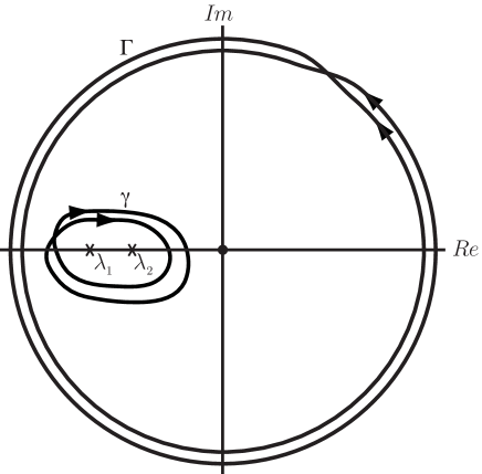
By Theorem 1.9, Proposition 3.6, and properties of limits of analytic functions, it suffices to consider the case that $|\lambda|$ and $|v_{+}|$ are arbitrarily small. Denote the Evans function for a given $v_{+}$ as $D^{v_{+}}$, suppressing other parameters. By Lemmas 2.9, and 3.3, we may for $v_{+}$ sufficiently small extend $D^{v_{+}}$ meromorphically to a ball $B(0,r)$ about $\lambda=0$, and the resulting extension is analytic (multi-valued) except at a pair of branch singularities $\lambda_{1}$ and $\lambda_{2}$ at which $D^{v_{+}}$ behaves as $d_{j}(\lambda-\lambda_{j})^{-1/4}$ for complex constants $d_{j}$. Making a branch cut on the segment between $\lambda_{1}$ and $\lambda_{2}$ as in Figure 5, we may view $\check{D}^{v_{+}}$ as an analytic function on a slit, two-sheeted Riemann surface obtained by circling the deleted segment $\overline{\lambda_{1}\lambda_{2}}$. Applying Proposition 3.6 again, we find that

$$D^{v_{+}}(\lambda)\sim D^{0}(\lambda)\sim c_{0}\lambda^{-1/2}+c_{1}$$

on $\partial B(0,r)$ as $v_{+}\to 0$, where $c_{j}$ are complex constants.

By Lemma 3.7, $c_{0}\neq 0$ for $B_{1}^{*}<\sqrt{\mu_{0}}$. For $B_{1}^{*}\geq\sqrt{\mu_{0}}$, $c_{0}\equiv 0$, and the condition that $\hat{D}^{0}\sim D^{0}$ not vanish at the origin is the condition that $c_{1}\neq 0$. Taking the winding number of $D^{v_{+}}$ around $\partial B(0,r)$, therefore, on the two-sheeted Riemann surface we have constructed– that is, circling twice as $D^{v_{+}}$ varies meromorphically– we obtain in the first place winding number negative one, and in the second (assuming $c_{1}\neq 0$) winding number zero. Subtracting the winding number about the segment $\overline{\lambda_{1}\lambda_{2}}$, necessarily greater than or equal to negative one by the asymptotics of $D^{v_{+}}$ at $\lambda_{j}$, we find by Cauchy’s Theorem/Principle of the Argument that for $B_{1}^{*}<\sqrt{\mu_{0}}$ there are no zeros of $\check{D}^{v_{+}}$ within $B(0,r)\setminus\overline{\lambda_{1}\lambda_{2}}$, concluding the proof in this case.

For $B_{1}^{*}\geq\sqrt{\mu_{0}}$, we find that there is at most one zero of $\check{D}^{v_{+}}$ within $B(0,r)\setminus\overline{\lambda_{1}\lambda_{2}}$. To complete the proof, we appeal as in [11] to the mod-two stability index of [16, 50, 51], which counts the parity of the number of unstable eigenvalues according to its sign, and is given by a nonzero real multiple of $D^{v_{+}}(0)$. To establish the theorem, it suffices to prove then that this stability index does not change sign, since we could then conclude stability by homotopy to a limiting stable case $\sigma\to+\infty$ or $B_{1}^{*}\to+\infty$. (Alternatively, we could check the sign by explicit computation, but we do not need to do so.) Recall that $D^{v_{+}}(0)$ is a nonvanishing real multiple of the product of the hyperbolic stability determinant and a transversality coefficient vanishing if and only if the traveling wave connection is not transverse.

As noted already in Proposition 1.4, the hyperbolic stability determinant does not vanish for Lax $3$-shocks, so is nonvanishing for $B_{1}^{*}>\sqrt{\mu_{0}}$. The transversality coefficient is an Evans function-like Wronskian of decaying solutions of the linearized traveling-wave ODE

$$\hat{v}^{-1}\begin{pmatrix}\mu_{0}&0\\ 0&1/\sigma\mu_{0}\end{pmatrix}\begin{pmatrix}\tilde{u}\\ \tilde{B}\end{pmatrix}^{\prime}=\begin{pmatrix}\mu_{0}&-B_{1}^{*}\\ -B_{1}^{*}&\hat{v}\end{pmatrix}\begin{pmatrix}\tilde{u}\\ \tilde{B}\end{pmatrix},$$ (3.14)

hence converges by Lemma 2.9 to the corresponding Wronskian for the limiting system with $\hat{v}$ replaced by $\hat{v}^{0}$. But, this limit must be nonzero wherever $c_{1}$ is nonzero, or else $\check{D}^{0}$ would vanish at $\lambda=0$ to at least order $\lambda$ due to a second linear dependence in decaying as well as asymptotically constant modes, and so $c_{1}=0$ in contradiction to our assumptions. Therefore, transversality holds by assumption for $0\leq B_{1}^{*}-\sqrt{\mu_{0}}\leq\max\{\sqrt{\frac{\mu_{0}}{2}},\sqrt{\frac{1}{2\sigma}}\,\}$ and $v_{+}$ sufficiently small.

On the other hand, an energy estimate like that of Section B.3 sharpened by the observation that $|\hat{v}^{0}_{x}|\leq\hat{v}$, improving the general estimate $\hat{v}_{x}\leq\gamma\hat{v}$, yields transversality of (3.14) for $B_{1}^{*}-\sqrt{\mu_{0}}\geq\max\{\sqrt{\frac{\mu_{0}}{2}},\sqrt{\frac{1}{2\sigma}}\,\}$. Thus, we have transversality for all $B_{1}^{*}\geq\sqrt{\mu_{0}}$, and we may conclude by homotopy to the stable $B_{1}^{*}\to\infty$ limit that the transversality coefficient has a sign consistent with stability, that is, there are an even number of nonstable zeros $\Re\lambda\geq 0$ of the Evans function $D^{v_{+}}$ for $v_{+}$ sufficiently small. Since we have already established that there is at most one nonstable zeros of $D^{v_{+}}$, this implies that there are no nonstable zeros, yielding stability as claimed. ∎

Figure 5: Winding number on two-sheeted Riemann surface.

Remark 3.9.

From Lemma 3.7, there might appear to be inherent numerical difficulty in verifying nonvanishing of $\check{D}$ for $B_{1}^{*}$ less than but close to $\sqrt{\mu_{0}}$, since $\check{D}$ vanishes at the origin for $B_{1}^{*}=\sqrt{\mu_{0}}$. However, this is only apparent, since we know analytically that $\check{D}^{0}$ does not vanish at, hence also near, $\lambda=0$ for $B_{1}^{*}<\sqrt{\mu_{0}}$.

4 Further asymptotic limits

In this section, we require beyond the conjugation lemma the further asymptotic ODE tools of the convergence and tracking/reduction lemmas of [38, 44]. Statements and proofs of these results are given for completeness in Appendix A.

4.1 The small-$\sigma$ and -$\mu_{0}$ limits

Proof of Theorem 1.16 ($\sigma\to 0$).

Considering (2.1) as indexed by $p:=\sigma$ with $A=A^{\sigma}$, we have (A.2)–(A.3) by uniform exponential convergence of $\hat{v}$ as $x\to\pm\infty$. Take without loss of generality $\mu=1$. Applying Lemma A.1, we find that the transformations $P^{\sigma}_{\pm}$ conjugating (2.1) to its constant-coefficient limits $Z^{\prime}=A^{\sigma}_{\pm}Z$, by which the Evans function is defined in (2.18), are given to $O(\sigma)$ by the transformations $P^{0}_{\pm}$ conjugating to its constant-coefficient limits the $\sigma=0$ system $W^{\prime}=A^{0}(x,\lambda)W$, with

$$A^{0}=\begin{pmatrix}0&1&0&0\\ \lambda\hat{v}&\hat{v}&0&0\\ 0&0&0&0\\ 0&-B_{1}^{*}\hat{v}&\lambda\hat{v}&0\end{pmatrix};$$ (4.1)

that is, $P^{\sigma}_{\pm}=P^{0}_{\pm}+O(\sigma)$. Moreover, for $v_{+}$ bounded from zero, and $\sigma/\lambda$ sufficiently small, it is straightforward to verify that the stable subspace of $A_{+}(\lambda,\sigma)$ is given to order $\sigma/\lambda$ by the span of $(r_{+},s_{+})^{T}$ and $(0,q_{+})^{T}$, where $r_{+}^{T}$ is the stable eigenvector of $\begin{pmatrix}0&1\\ \lambda\hat{v}&\hat{v}\end{pmatrix}$ and $q_{+}=(-\sqrt{\sigma\mu_{0}/\lambda},1)$, and, similarly, the unstable subspace of $A_{-}(\lambda,\sigma)$ is given to order $\sigma/\lambda$ by the span of $(r_{-},s_{-})^{T}$ and $(0,q_{-})^{T}$, where $r_{-}^{T}$ is the unstable eigenvector of $\begin{pmatrix}0&1\\ \lambda\hat{v}&\hat{v}\end{pmatrix}$ and $q_{-}=(\sqrt{\sigma\mu_{0}/\lambda},1)$. Thus, the Evans function for $\sigma>0$, appropriately rescaled, is within $O(\sigma/\lambda)$ of the product of the Evans function of the diagonal block $w^{\prime}=\begin{pmatrix}0&1\\ \lambda\hat{v}&\hat{v}\end{pmatrix}w$ initialized in the usual way, which is nonzero by our earlier analysis of the decoupled case $B_{1}^{*}=0$, and of the trivial flow

$$w^{\prime}=\hat{v}(x)\begin{pmatrix}0&0\\ \lambda&0\end{pmatrix}w$$ (4.2)

initialized with vectors parallel to $q\pm^{T}$ in the conjugated flow. To estimate the second determinant, we produce explicit conjugators $P^{0}_{\pm}$ for the $\sigma=0$ flow, making use of the observation of Remark 2.10 that, by lower block-triangular form of the $A^{0}$, these may be taken lower block-triangular as well, and so the problem reduces to finding conjugators $p^{0}_{\pm}$ for the flow (4.2) in the lower block. But, these may be found by exponentiation to be

$$p^{0}_{\pm}=\begin{pmatrix}1&0\\ c_{\pm}(x)&1\end{pmatrix},\qquad c_{\pm}(x):=\int_{x}^{\pm\infty}(\hat{v}-v_{\pm})(y)dy,$$

yielding an Evans function to order $\sigma/\lambda$ of

$$\det(p^{0}_{-}q_{-},p^{0}_{+}q_{+})=\det\begin{pmatrix}\sqrt{\sigma\mu_{0}/\lambda}&-\sqrt{\sigma\mu_{0}/\lambda}\\ 1+c_{-}(0)\sqrt{\sigma\mu_{0}/\lambda}&1-c_{+}\sqrt{\sigma\mu_{0}/\lambda}\end{pmatrix},$$

or

$$(1+O(\sqrt{\sigma/\lambda}))2\sqrt{\sigma\mu_{0}/\lambda}\neq 0.$$

In particular, the Evans function is nonvanishing for $1\gg|\sqrt{\sigma/\lambda}|\gg|\sigma|,\,|\sigma/\lambda|$, as occurs for

$$\sigma\ll|\lambda|\ll\sigma^{-1}.$$

Since the Evans function is nonvanishing in any case for $|\lambda|$ sufficiently large, by Theorem 1.9, we obtain nonvanishing except in the case $0\leq|\lambda|\leq C\sigma$, which must be treated separately.

To treat $|\lambda|\leq C\sigma$, notice that the stable/unstable subspaces of $A^{\sigma}_{\pm}$ decouple to order $\sigma$ for $\sigma>0$ sufficiently small and $\lambda$ only bounded into the direct sum of $(r,s)_{\pm}^{T}$ already discussed and $(0,\tilde{q}_{\pm})^{T}$ with $\tilde{q}_{\pm}^{T}$ the stable/unstable eigenvectors of

$$\begin{pmatrix}0&1\\ \lambda/\sigma\mu_{0}&\sigma\mu_{0}v\end{pmatrix},$$

which may be chosen holomorphically as $\tilde{q}_{\pm}=(1,\sigma\mu_{0}/2\mp\sqrt{\sigma^{2}\mu_{0}^{2}/4+\lambda/\sigma\mu_{0}})$, with a single square-root singularity at $\lambda=-(\sigma\mu_{0})^{3}/4$. For $|\lambda|\geq C\sigma$, these factor as

$$\tilde{q}_{\pm}=(1+O(\sigma/\lambda))(1,\mp\sqrt{\lambda/\sigma\mu_{0}})=(1+O(\sigma/\lambda))(\sqrt{\lambda/\sigma\mu_{0}})q_{\pm},$$

and the Evans function for $\sigma>0$ by our previous computations thus satisfies

$$D^{\sigma}(\lambda)=(\lambda/\sigma\mu_{0})\times(1+O(\sqrt{\sigma/\lambda}))2e^{c_{-}(0)+c_{+}(0)}\sqrt{\sigma\mu_{0}/\lambda}\sim C\sqrt{\lambda/\sigma\mu_{0}}.$$

Taking the winding number about $|\lambda|=C\sigma$ on the punctured Riemann surface obtained by circling twice the branch singularity $\lambda_{*}=(\sigma\mu_{0})^{3}/4$, we thus obtain winding number one. Subtracting the nonnegative winding number obtained by circling twice infinitesimally close to $\lambda_{*}$, we find (similarly as in the treatment of the large-amplitude limit, case $B_{1}^{*}\geq\sqrt{\mu_{0}}$) that there is at most one root of $D^{\sigma}$ on $\Re\lambda\geq 0$, for $\sigma>0$ sufficiently small, so that stability is decided by the sign of the stability index, which is the product of a transversality coefficient and the hyperbolic stability determinant (resp. low-frequency stability condition, in the overcompressive case). A singular perturbation analysis of (B.4) as $\sigma\to 0$ shows that (since it decouples into scalar fibers) connections are always transverse for $\sigma>0$, so the transversality coefficient does not vanish. Hyperbolic stability holds always for Lax $1$- and $3$-shocks (Proposition 1.4), and the low-frequency stability condition holds for intermediate (overcompressive) shocks by a similar singular perturbation analysis, so the stability determinant does not vanish either.

Thus, the sign of the stability index is constant, and so there is always either a single unstable root of $D^{\sigma}$ on $\Re\lambda\geq 0$ or none, in each of the three cases. But, the former possibility may be ruled out by homotopy to the stable, small-amplitude limiting case. Thus, all type shocks are reduced Evans stable for $\sigma>0$ sufficiently small. The asserted $\sqrt{\sigma}$ asymptotics follow from the estimates already obtained in the proof; uniform convergence to zero follows by estimating $D^{\sigma}$ instead to order $\sqrt{\sigma}$, at which level we obtain a determinant involving two copies of the constant solution $W\equiv(0,0,0,1)^{T}$ of the limiting $\sigma=0$ system, giving zero as the limiting value. ∎

Proof of Theorem 1.16 ($\mu_{0}\to 0$).

The case $\mu_{0}\to 0$ is similar to but a bit tricker than the case $\sigma\to 0$ just discussed. Fixing without loss of generality $\mu=1$ and applying Lemma A.1, we deduce that the transformations $P^{\mu_{0}}_{\pm}$ conjugating (2.1) to its limiting constant-coefficient systems, by which the Evans function is defined in (2.18), satisfy $P^{\mu_{0}}_{\pm}=P^{0}_{\pm}+O(\mu_{0})$, where $P^{0}_{\pm}$ are the transformations conjugating to its constant-coefficient limits the upper block-triangular $\mu_{0}=0$ system

$$\begin{pmatrix}W_{1}\\ W_{2}\\ W_{4}\\ W_{3}\end{pmatrix}^{\prime}=\begin{pmatrix}0&1&0&0\\ \lambda\hat{v}&\hat{v}&-\sigma B_{1}^{*}\hat{v}&0\\ 0&-B_{1}^{*}\hat{v}&0&\lambda\hat{v}\\ 0&0&0&0\\ \end{pmatrix}\begin{pmatrix}W_{1}\\ W_{2}\\ W_{4}\\ W_{3}\end{pmatrix},$$ (4.3)

which has a constant right zero-eigenvector $r=(\sigma B_{1}^{*},0,\lambda,0)^{T}$ and an orthogonal constant left zero-eigenvector $\ell=(0,0,0,1)^{T}$, signaling a Jordan block at eigenvalue zero. It is readily checked for the limiting matrices at $\pm\infty$, similarly as in the $\sigma\to 0$ case, that for $\mu_{0}/\lambda$ sufficiently small, the Jordan block splits to order $\sim\sqrt{\mu_{0}/\lambda}$, so that the “slow” stable eigenvector at $+\infty$ (that is, the one with eigenvalue near zero) is given by

$$r+c_{+}\sqrt{\mu_{0}/\lambda}(*,*,*,1)^{T}+O(\mu_{0}/\lambda),$$

and the slow unstable eigenvector at $-\infty$ by

$$r+c_{-}\sqrt{\mu_{0}/\lambda}(*,*,*,1)^{T}+O(\mu_{0}/\lambda),$$

where $c_{\pm}$ are constants with a common sign. (Here, we deduce nonvanishing of the final coordinate of the second summand without computation by noting that the dot product with $\ell$ must be $\sim\sqrt{\mu_{0}/\lambda}$.)

As for the $\sigma\to 0$ case, we now observe that (4.3) may be conjugated to constant-coefficients by block-triangular conjugators $P_{\pm}=\begin{pmatrix}p_{\pm}&q_{\pm}\\ 0&1\end{pmatrix}$, where $p_{\pm}$ conjugate the upper lefthand block system

$$\begin{pmatrix}W_{1}\\ W_{2}\\ W_{4}\end{pmatrix}^{\prime}=\begin{pmatrix}0&1&0\\ \lambda\hat{v}&\hat{v}&-\sigma B_{1}^{*}\hat{v}\\ 0&-B_{1}^{*}\hat{v}&0\\ \end{pmatrix}\begin{pmatrix}W_{1}\\ W_{2}\\ W_{4}\end{pmatrix}.$$ (4.4)

Moreover, changing coordinates to lower block-triangular form

$$\begin{pmatrix}W_{1}\\ W_{2}\\ W_{4}-\lambda W_{1}/\sigma B_{1}^{*}\end{pmatrix}^{\prime}=\begin{pmatrix}0&1&0\\ 0&\hat{v}&-\sigma B_{1}^{*}\hat{v}\\ 0&-B_{1}^{*}\hat{v}-\lambda/\sigma B_{1}^{*}&0\\ \end{pmatrix}\begin{pmatrix}W_{1}\\ W_{2}\\ W_{4}-\lambda W_{1}/\sigma B_{1}^{*}\end{pmatrix},$$ (4.5)

conjugating by a lower block-triangular conjugator, and changing back to the original coordinates, we see that the conjugators $p_{\pm}$ may be chosen to preserve the exact solution $(W_{1},W_{2},W_{4},W_{3})^{T}\equiv r$.

Combining these observations, we find that the Evans function for $\lambda$ bounded and $\mu_{0}/\lambda$ sufficiently small is given by

$$D^{\mu_{0}}(\lambda) =\det\begin{pmatrix}\tilde{r}&v_{2}^{-}&v_{2}^{+}&\tilde{r}\\ c_{-}\sqrt{\mu_{0}/\lambda}&0&0&-c_{+}\sqrt{\mu_{0}/\lambda}\\ \end{pmatrix}+O(\mu_{0}/\lambda)$$ (4.6)

$$=\det\begin{pmatrix}0&v_{2}^{-}&v_{2}^{+}&\tilde{r}\\ (c_{-}+c_{+})\sqrt{\mu_{0}/\lambda}&0&0&c_{+}\sqrt{\mu_{0}/\lambda}\\ \end{pmatrix}+O(\mu_{0}/\lambda)$$

$$=(c_{-}+c_{+})\sqrt{\mu_{0}/\lambda}d(\lambda)+O(\mu_{0}/\lambda),$$

where $r=:\begin{pmatrix}\tilde{r}\\ 0\end{pmatrix}$ and $d(\lambda):=\det\begin{pmatrix}v_{2}^{-}&v_{3}^{+}&\tilde{r}\end{pmatrix}$ is a nonstandard Evans function associated with the upper-block system (4.4), where $v_{2}^{-}$ and $v^{+}_{3}$ as usual are unstable and stable eigendirections of the coefficient matrix, but we have included also the neutral mode $\tilde{r}$. Expressed in coordinate (4.5), $d(\lambda)$ reduces, finally, to the standard Evans function $\check{d}(\lambda)$ for the reduced system

$$\begin{pmatrix}W_{2}\\ W_{4}-\lambda W_{1}/\sigma B_{1}^{*}\end{pmatrix}^{\prime}=\begin{pmatrix}\hat{v}&-\sigma B_{1}^{*}\hat{v}\\ -B_{1}^{*}\hat{v}-\lambda/\sigma B_{1}^{*}&0\\ \end{pmatrix}\begin{pmatrix}W_{2}\\ W_{4}-\lambda W_{1}/\sigma B_{1}^{*}\end{pmatrix},$$

which may be rewritten as a second order equation

$$\big{(}\lambda+\sigma(B_{1}^{*})^{2}\big{)}z+z^{\prime}=(z^{\prime}/\hat{v})^{\prime}$$ (4.7)

in $z=W_{2}^{\prime}$. Taking the real part of the complex $L^{2}$-inner product of $z$ against (4.7) gives

$$\Re\lambda\|v\|_{L^{2}}^{2}+\|v\sqrt{\big{(}\Re\lambda+\sigma(B_{1}^{*})^{2}\big{)}}\|_{L^{2}}^{2}=-\|v^{\prime}/\sqrt{\hat{v}}\|_{L^{2}}^{2},$$

contradicting the existence of a decaying solution for $\Re\lambda\geq 0$ and verifying that $\check{d}(\lambda)\neq 0$. Consulting (4.6), therefore, we find that $D^{\mu_{0}}(\lambda)$ for $\lambda$ bounded and $\mu_{0}/\lambda$ sufficiently small does not vanish and, moreover, $D^{\mu}_{0}\sim c\sqrt{\mu_{0}/\lambda}$ for $\lambda$ sufficiently small, $c\neq 0$ constant. Performing a Riemann surface winding number computation like that for the case $\sigma\to 0$, we find, finally, that $D^{\mu_{0}}$ does not vanish for any $\Re\lambda\geq 0$. We omit the details of this last step, since they are essentially identical to those in the previous case. Likewise, the asserted asymptotics follow exactly as before. ∎

4.2 The large- and small-$B_{1}^{*}$ limits

Proof of Theorem 1.15.

Stability in the small-$B_{1}^{*}$ limit follows readily by continuity of the Evans function with respect to parameters, the high-frequency bound of Theorem 1.9, and the zero-$B_{1}^{*}$ stability result of Proposition B.1. We now turn to the large-$B_{1}^{*}$ limit. Let us rearrange (2.1), $\mu=1$, to

$$\begin{pmatrix}w\\ \alpha\\ w^{\prime}\\ \frac{\alpha^{\prime}}{\sigma\mu_{0}\hat{v}}\end{pmatrix}^{\prime}=\begin{pmatrix}0&0&1&0\\ 0&0&0&\sigma\mu_{0}\hat{v}\\ \lambda\hat{v}&0&\hat{v}&-\sigma B_{1}^{*}\hat{v}\\ 0&\lambda\hat{v}&-B_{1}^{*}\hat{v}&\sigma\mu_{0}\hat{v}^{2}\\ \end{pmatrix}\begin{pmatrix}w\\ \alpha\\ w^{\prime}\\ \frac{\alpha^{\prime}}{\sigma\mu_{0}\hat{v}}\end{pmatrix},$$ (4.8)

By Theorem 1.9, we have stability for $|\lambda|\geq C|B_{1}^{*}|^{2}$ independent of $v_{+}$. For $v_{+}>0$, we find easily stability for $|\lambda|\geq C|B_{1}^{*}|$ for $B_{1}^{*}$ sufficiently large. For, rescaling $x\to|B_{1}^{*}|x$, and $W\to(\lambda^{1/2}W_{1},\lambda^{1/2}W_{2},W_{3},W_{4})^{T}$, we obtain $W^{\prime}=\hat{A}W=\hat{A}_{0}W+O(|B_{1}^{*}|^{-1})W$, where

$$\hat{A}_{0} =\begin{pmatrix}0&0&\hat{\lambda}^{1/2}&0\\ 0&0&0&\hat{\lambda}^{1/2}\sigma\mu_{0}\hat{v}\\ \hat{\lambda}^{1/2}\hat{v}&0&0&-\sigma\hat{v}\\ 0&\hat{\lambda}^{1/2}\hat{v}&-v&0\\ \end{pmatrix},$$ (4.9)

with $\hat{\lambda}^{1/2}:=\lambda^{1/2}/B_{1}^{*}$, and $\hat{v}=\bar{v}(x/B_{1}^{*})$, $\bar{v}$ independent of $B_{1}^{*}$.

For $\hat{\lambda}\gg|B_{1}^{*}|^{-1}$ it is readily calculated that $\hat{A}_{0}$ has spectral gap $\gg|B_{1}^{*}|^{-1}$ for $\Re\lambda\geq 0$. Indeed, splitting into cases $\hat{\lambda}\geq C^{-1}$ and $\hat{\lambda}\ll 1$, it is readily verified in the first case by standard matrix perturbation theory that there exist matrices $R(\hat{v}(x))$ and $L=R^{-1}$, both smooth functions of $\hat{v}$, such that

$$L\hat{A}_{0}R=D:=\begin{pmatrix}M&0\\ 0&N\end{pmatrix},$$

with $\Re M\geq\theta>0$ and $\Re N\leq-\theta<0$. Making the change of coordinates $W=RZ$, we obtain the approximately block-diagonal equations $Z^{\prime}=\tilde{A}Z$, where

$$\tilde{A}:=LAR-L^{\prime}R=D+O(|B_{1}^{*}|^{-1}).$$ (4.10)

Using the tracking/reduction lemma, Lemma A.4, we find that there exist analytic functions $z_{2}=\Phi_{2}(z_{1})=O(r)$ and $z_{1}=\Phi_{1}(z_{2})=O(r)$ such that $(z_{1},\Phi_{2}(z_{1})$ and $(\Phi_{1}(z_{2}),z_{2})$ are invariant under the flow of (4.16), hence represent decoupled stable and unstable manifolds of the flow. But, this implies that the Evans function is nonvanishing on $\lambda\in\{\Re\lambda\geq 0\}$ for $B_{1}^{*}$ sufficiently large and $|\lambda|^{1/2}\geq|B_{1}^{*}|/C$, for any fixed $C>0$. See [55, 38, 50] for similar arguments.

If $|\lambda^{1/2}|\ll B_{1}^{*}$ on the other hand, or, equivalently, $|\hat{\lambda}^{1/2}|\ll 1$, then we can decompose $\hat{A}$ alternatively as $W^{\prime}=\hat{A}W=\hat{B}_{0}W+\hat{\lambda}^{1/2}B_{1}W+O(|B_{1}^{*}|^{-1})$, where

$$\hat{B}_{0} =\begin{pmatrix}0&0&0&0\\ 0&0&0&0\\ 0&0&0&-\sigma\hat{v}\\ 0&0&-v&0\\ \end{pmatrix},\qquad\hat{B}_{1} =\begin{pmatrix}0&0&1&0\\ 0&0&0&\sigma\mu_{0}\hat{v}\\ \hat{v}&0&0&0\\ 0&\hat{v}&0&0\\ \end{pmatrix}.$$ (4.11)

By smallness of $\hat{\lambda}^{1/2}$ together with spectral separation between the diagonal blocks of $\hat{B}_{0}$, there exist $L$, $R$, $LR\equiv 0$ such that the transformation $W=RZ$ takes the system to $Z^{\prime}=(LBR-L^{\prime}R)Z=CZ+O(|B_{1}^{*}|^{-1})\Theta$, where $\Theta=\begin{pmatrix}0&*\\ &*\\ \end{pmatrix}$ and

$$C=\begin{pmatrix}-\hat{\lambda}\beta^{-1}+O(\hat{\lambda}^{2})&0\\ 0&\hat{\beta}\end{pmatrix},\qquad\beta=\begin{pmatrix}0&-1/\mu_{0}\hat{v}\\ -1&0\\ \end{pmatrix},\qquad\hat{\beta}=\begin{pmatrix}0&-\sigma\hat{v}\\ -v&0\\ \end{pmatrix}.$$ (4.12)

Diagonalizing $\beta$ into growing and decaying mode by a further transformation, and applying the tracking lemma again, we may decouple the equations into a scalar uniformly-growing mode, a scalar uniformly-decaying mode, and a $2$-dimensional mode governed by

$$z^{\prime}=-\hat{\lambda}\beta^{-1}z+O(|B_{1}^{*}|^{-2}+|\hat{\lambda}^{2}|)z.$$ (4.13)

If $\hat{\lambda}\gg|B_{1}^{*}|^{-1}$, or, equivalently, $|\lambda|\gg|B_{1}^{*}|$, then we make a further transformation diagonalizing $\beta^{-1}$ at the expense of an $O(|B_{1}^{*}|^{-1})$ error, then use the resulting $\geq|\hat{\lambda}|$ spectral gap together with the tracking lemma to again conclude nonvanishing of the Evans function.

Thus, we may restrict to the case $|\lambda|\leq C|B_{1}^{*}|$, or $|\hat{\lambda}|\leq C|B_{1}^{*}|^{-1}$. Considering again (4.13) in this case, we find that all $O(|B_{1}^{*}|^{-2}+|\hat{\lambda}^{2}|)$ entries converge at rate

$$O(|B_{1}^{*}|^{-2})|\hat{v}-v_{+}|\leq C|B_{1}^{*}|^{-2}e^{-|x|/CB_{1}^{*}}$$

to limiting values, whence, by the convergence lemma, Lemma A.1, the Evans function for the reduced system (4.13) converges to that for $z^{\prime}=-\hat{\lambda}\beta^{-1}z$ as $B_{1}^{*}\to\infty$. But, this equation, written in original coordinates, is exactly the eigenvalue equation for the reduced inviscid system

$$\lambda\begin{pmatrix}w\\ \alpha\end{pmatrix}+\begin{pmatrix}0&-B_{1}^{*}/\mu_{0}\hat{v}\\ -B_{1}^{*}&0\end{pmatrix}\begin{pmatrix}w\\ \alpha\end{pmatrix}^{\prime}=0,$$ (4.14)

which may be shown stable by an energy estimate as in the case $\sigma=0$.

Finally, noting that the decoupled fast equations are independent of $\lambda$ to lowest order, we find for $|\lambda|$ bounded and $B_{1}^{*}\to\infty$ that the Evans function (which decomposes into the product of the decoupled Evans functions) converges to a constant multiple of the Evans function for (4.14). For $|\lambda|\leq C$, or $\hat{\lambda}\leq C|B_{1}^{*}|^{-2}$, however, we may apply to (4.13) the convergence lemma, Lemma A.1, together with Remark A.3, to see that the Evans function in fact converges to that for the piecewise constant-coefficient equations obtained by substituting for the coefficient matrix on $x\gtrless 0$ its asymptotic values at $\pm\infty$, that is, the determinant $d:=\det(r^{+},r^{-})$, where $r^{+}$ is the stable eigenvector of

$$\begin{pmatrix}0&-B_{1}^{*}/\mu_{0}\hat{v}\\ -B_{1}^{*}&0\end{pmatrix}$$

at $+\infty$ and $r^{-}$ is the unstable eigenvector at $-\infty$. Computing, we have $r^{\pm}=(1,\mp\sqrt{\mu_{0}v_{\pm}})^{T}$ where giving a constant limit $d=\sqrt{\mu_{0}v_{+}}+\sqrt{\mu_{0}}$ as claimed. ∎

4.3 The large-$\sigma\mu_{0}$ limit

Proof of Theorem 1.17.

By Theorem 1.9, it is sufficient to treat the case $|\lambda|\leq C\sigma\mu_{0}$. Decompose (2.1), $\mu=1$, as $W^{\prime}=RA_{0}+A_{1}$, where $R:=\sigma\mu_{0}$, $\hat{\lambda}:=\lambda/R$, and

$$A_{0}=\begin{pmatrix}0&0&0&0\\ \hat{\lambda}\hat{v}&0&0&-B_{1}^{*}\hat{v}/\mu_{0}\\ 0&0&0&\hat{v}\\ 0&0&\hat{\lambda}\hat{v}&\hat{v}^{2}\end{pmatrix},\qquad A_{1}=\begin{pmatrix}0&1&0&0\\ 0&\hat{v}&0&0\\ 0&0&0&0\\ 0&-B_{1}^{*}\hat{v}&0&0\\ \end{pmatrix},$$

with $|A_{1}|\leq C$. If $|\hat{\lambda}|\geq 1/C>0$, then the lower $2\times 2$ righthand block of $A_{0}$ has eigenvalues $\pm\hat{v}\sqrt{\hat{\lambda}}$ uniformly bounded from the eigenvalues zero of the upper lefthand $2\times 2$ block. By standard matrix perturbation theory, therefore, there exist well-conditioned coordinate transformations $L$, $R$ depending smoothly on $\hat{v}$ such that

$$D:=LA_{0}R=\begin{pmatrix}0&0&0&0\\ \hat{\lambda}\hat{v}&0&0&0\\ 0&0&\hat{v}\sqrt{\hat{\lambda}}&0\\ 0&0&0&-\hat{v}\sqrt{\hat{\lambda}}\\ \end{pmatrix}.$$

Making the coordinate transformation $W=RZ$, we obtain $Z^{\prime}=DZ+O(1)Z$. Applying the tracking lemma, Lemma A.4, we reduce to a system of three decoupled equation, consisting of a uniformly growing scalar equation, a uniformly decaying scalar equation, and a $2\times 2$ equation $z^{\prime}=\begin{pmatrix}0&1\\ R\hat{\lambda}\hat{v}&0\end{pmatrix}z+O(R^{-1})z.$ Rescaling by $z:=\begin{pmatrix}1&0\\ 0&R^{1/2}\end{pmatrix}y$, we obtain $y^{\prime}=R^{1/2}\begin{pmatrix}0&1\\ \hat{\lambda}\hat{v}&0\end{pmatrix}y+O(R^{-1/2})y,$ which, by a second application of the tracking lemma, may be reduced to a pair of decoupled, uniformly growing/decaying scalar equations, thus completely decoupling the original system into four growing/decaying scalar equations, from which we may conclude nonvanishing of the Evans function.

It remains to treat the case $|\hat{\lambda}|\ll 1$. We decompose (2.1), $\mu=1$, in this case as $W^{\prime}=RB_{0}+B_{1}$, where

$$B_{0}=\begin{pmatrix}0&0&0&0\\ 0&0&0&-B_{1}^{*}\hat{v}/\mu_{0}\\ 0&0&0&\hat{v}\\ 0&0&0&\hat{v}^{2}\end{pmatrix},\qquad B_{1}=\begin{pmatrix}0&1&0&0\\ \lambda\hat{v}&\hat{v}&0&0\\ 0&0&0&0\\ 0&-B_{1}^{*}\hat{v}&\lambda\hat{v}&0\\ \end{pmatrix},$$

with $|\lambda|\ll R$. Defining $T=\begin{pmatrix}I&\theta\\ 0&I\end{pmatrix}$ where $\theta=(0,-B_{1}^{*}\hat{v}/\mu_{0},\hat{v})^{T}$, and making the change of variables $W=TZ$, we obtain $Z^{\prime}=RC_{0}Z+C_{1}Z$, where

$$C_{0}=\begin{pmatrix}c_{0}&0\\ 0&\hat{v}^{2}+\frac{\hat{v}^{2}}{R}\Big{(}\frac{(B_{1}^{*})^{2}}{\mu_{0}}+\lambda\Big{)}\end{pmatrix},\>\;c_{0}=\beta-\theta x=\begin{pmatrix}0&1&0\\ \lambda\hat{v}&\hat{v}-(B_{1}^{*})^{2}\hat{v}^{2}/\mu_{0}&\lambda(B_{1}^{*})^{2}\hat{v}^{2}/\mu_{0}\\ 0&-B_{1}^{*}\hat{v}^{2}&\lambda\hat{v}^{2}\\ \end{pmatrix},$$

and

$$\beta=\begin{pmatrix}0&1&0\\ \lambda\hat{v}&\hat{v}&0\\ 0&0&0\\ \end{pmatrix},\qquad x=\begin{pmatrix}0&-B_{1}^{*}\hat{v}&\lambda\hat{v}\end{pmatrix},\qquad C_{1}=\begin{pmatrix}0&*\\ *&0\end{pmatrix}=O(1).$$

Applying the tracking lemma, we reduce to a decoupled system consisting of a uniformly growing scalar equation

$$y^{\prime}=(R+\frac{(B_{1}^{*})^{2}}{\mu_{0}}+\lambda)\hat{v}^{2}y+O(1/R)y$$ (4.15)

associated with the lower right diagonal entry and a $3\times 3$ system

$$z^{\prime}=c_{0}z+O(1/R)z.$$

For $|\lambda|\gg 1$, we may write $c_{0}=\begin{pmatrix}0&1&*\\ \lambda\hat{v}&0&*\\ 0&0&\lambda\hat{v}^{2}\\ \end{pmatrix}+O(1),$ and apply the tracking lemma again to obtain three decoupled equations uniformly growing/decaying at rates $\pm\sqrt{\lambda\hat{v}}$ and $\lambda\hat{v}^{2}$, giving nonvanishing of the Evans function. For $|\lambda|\leq C$ on the other hand, we may apply the convergence lemma, Lemma A.1, using the fact that the $O(1/R)$ coefficient converges to its limits as $CR^{-1}e^{-\eta|x|}$, $\eta>0$, together with Remark A.3, to obtain convergence to the unperturbed system $z^{\prime}=c_{0}z$. But, this may be recognized as exactly the formal limiting system (1.21) for ($\sigma=\infty$), which is stable by Theorem 1.7 (established by energy estimates). Noting that the Evans function for the full system is the product of the Evans functions of its decoupled components, and that The Evans function for the scalar component converges likewise to that for $y^{\prime}=(R+\frac{(B_{1}^{*})^{2}}{\mu_{0}}+\lambda)\hat{v}^{2}y$, or (by direct computation/exponentiation) $d(\lambda)=e^{c_{0}R+c_{1}+c_{2}\lambda}$ for constants $c_{j}$, we find, finally, that the full Evans function after renormalization by factor $e^{-c_{0}R}$ converges to a constant multiple of the Evans function for (1.21). ∎

4.4 The limit as $\mu/(2\mu+\eta)\to 0$ or $\to\infty$

Finally, we briefly discuss the effect of dropping the gas-dynamical assumption $\eta=-4\mu/3$, and considering more general values of $(2\mu+\eta)>0$. This parameter does not appear in the transverse equations, so enters only indirectly to our analysis, through its effect on the gas-dynamical profile $\hat{v}(x)$. Specifically, denoting $r:=\mu/(2\mu+\eta)\to 0$, and taking as usual the normalization $\mu=1$, we find that

$$\hat{v}(x)=\bar{v}(rx),$$

where $\bar{v}$ is a profile independent of the value of $r$. Thus, the study in [13] of the limit $r\to 0$ is the limit of slowly-varying coefficients, and the opposite limit $r\to\infty$ is the limit rapidly-varying coefficients. We consider each of these limiting cases in turn. Intermediate values of $\mu/(2\mu+\eta)$ would presumably need to be studied numerically, an interesting direction for further investigation.

4.4.1 The $r\to 0$ limit

In the $r\to 0$ limit, we have the following result completing the analysis of [13]

Proposition 4.1.

Parallel isentropic MHD shocks with ideal gas equation of state are reduced Evans stable in the limit as $r\to 0$ with other parameters held fixed.

Proof.

The case $B_{1}^{*}<2\sqrt{\mu_{0}}$ including Lax $1$-type, overcompressive type, and some Lax $3$-type shocks has been established in [13] by energy estimates. Thus, it suffices to treat the case of Lax $3$-shocks and (by Proposition 1.9) bounded $|\lambda|$.

For shocks of any type, it is straightforward to verify that the Evans function is nonvanishing on $\lambda\in\{\Re\lambda\geq 0\}\setminus B(0,\varepsilon)$, any $\varepsilon>0$, for $r$ sufficiently small. For, on this set of $\lambda$, there is a uniform spectral gap between the real parts of the stable and unstable eigenvalues of $A(x,\lambda)$, for all $x\in(-\infty,+\infty)$, by the hyperbolic-parabolic structure of the equations, similarly as in Lemma 2.1. It follows by standard matrix perturbation theory that there exist matrices $R(\hat{v}(x))$ and $L=R^{-1}$ such that

$$LAR=D:=\begin{pmatrix}M&0\\ 0&N\end{pmatrix},$$

with $\Re M\geq\theta>0$ and $\Re N\leq-\theta<0$. Making the change of coordinates $W=RZ$, we obtain the approximately block-diagonal equations

$$Z^{\prime}=\tilde{A}Z,$$ (4.16)

where

$$\tilde{A}:=LAR-L^{\prime}R=D+O(\hat{v}_{x})=D+O(r\bar{v}_{x}).$$ (4.17)

Using the tracking/reduction lemma, Lemma A.4, we find that there exist analytic functions $z_{2}=\Phi_{2}(z_{1})=O(r)$ and $z_{1}=\Phi_{1}(z_{2})=O(r)$ such that $(z_{1},\Phi_{2}(z_{1})$ and $(\Phi_{1}(z_{2}),z_{2})$ are invariant under the flow of (4.16), hence represent decoupled stable and unstable manifolds of the flow. But, this implies that the Evans function is nonvanishing on $\lambda\in\{\Re\lambda\geq 0\}\setminus B(0,\varepsilon)$, any $\varepsilon>0$, for $r$ sufficiently small. See [55, 38, 50] for similar arguments.

Now, restrict to the case of a Lax $3$-shock for $\lambda\in\{\Re\lambda\geq 0\}\cap B(0,\varepsilon)$ and $\varepsilon>0$ sufficiently small. By examination of $A(x,\lambda)$ at $\lambda=0$ in the Lax $3$-shock case, we find that on $B(0,\varepsilon)$ it has one eigenvalue $\mu_{+}$ that is uniformly negative, one eigenvalue $\mu_{-}$ that is uniformly positive, and two that are small. By standard matrix perturbation theory [38, 50], there exist matrices $L=\begin{pmatrix}L_{+}\\ L_{0}\\ L_{-}\end{pmatrix}$, $R=\begin{pmatrix}R_{+}&R_{0}&R_{-}\end{pmatrix}$ with $LR\equiv I$ and $L_{j}^{\prime}R_{j}\equiv 0$ such that

$$LAR(x,\lambda)=\begin{pmatrix}\mu_{+}&0&0\\ 0&\lambda M_{0}&0\\ 0&0&\mu_{-}\end{pmatrix},$$

where the crucial factor $\lambda$ in $\lambda M_{0}$ is found by explicit computation/Taylor expansion [55, 38, 50, 41], and $M_{0}=-\beta^{-1}+O(\lambda)$, where $\beta$ as in (2.5) is the hyperbolic convection matrix

$$\beta:=\begin{pmatrix}1&-B_{1}^{*}/\mu_{0}\hat{v}\\ -B_{1}^{*}&1\end{pmatrix}.$$ (4.18)

Moreover, $R$, $L$ depend only on $\hat{v}$, $\lambda$. Making the change of coordinates $Z:=LW$, we obtain $Z^{\prime}=B(x,\lambda)Z$, where

$$B=LAR-L^{\prime}R=\begin{pmatrix}\mu_{+}&O(\hat{v}_{x})&O(\hat{v}_{x})\\ O(\hat{v}_{x})&\lambda M_{0}&O(\hat{v}_{x})\\ O(\hat{v}_{x})&O(\hat{v}_{x})&\mu_{-}\end{pmatrix}.$$

Applying the tracking/reduction lemma again, we reduce to three decoupled equations associated with the three diagonal blocks. The two scalar equations associated with $\mu_{\pm}$ are uniformly growing/decaying, so do not support nontrivial decaying solutions at both infinities. Thus, vanishing of the Evans function reduces to vanishing or nonvanishing on the central block

$$w^{\prime}=(\lambda M_{0}+O(\hat{v}_{x}^{2}))w,$$

$w\in{\mathbb{C}}^{2}$. Noting that $\|\hat{v}_{x}^{2}\|_{L^{1}}=O(r)\to 0$, we may apply the convergence lemma, Lemma A.1, together with Remark A.3, to reduce finally to

$$z^{\prime}=\lambda M_{0}z,\quad M_{0}:=L_{0}AR_{0}.$$ (4.19)

For $|\lambda|\ll r$, we have $|\lambda M_{0}-\lambda M_{0}(+\infty)|\leq C\lambda e^{-\theta r}$, hence

$$\|\lambda M_{0}-\lambda M_{0}(+\infty)\|_{L^{1}[0,+\infty)}=O(\lambda/r)\to 0$$

and we may apply the conjugation lemma to obtain that the Evans function for the reduced central system (4.19) is given by $(1+O(\lambda/r))\det(r_{-},r_{+})$, where $r_{-}$ is an unstable eigenvalue of $M_{0}(-\infty)$ and $r_{+}$ is a stable eigenvalue of $M_{0}(-\infty)$. Noting that these to order $\lambda$ are stable/unstable eigenvectors of $\beta_{\pm}$, we find by direct computation that the determinant does not vanish. Indeed, this is exactly the computation that the Lopatinski determinant does not vanish for $3$-shocks. Thus, we may conclude that the Evans function does not vanish for $|\lambda|\ll r$.

Finally, we consider the remaining case $r/C\leq|\lambda|\leq Cr$, for $C>0$ large but fixed. In this case, we may for the same reason drop terms of order $\lambda^{2}$ in the expansion of $\lambda M_{0}$, to reduce by an application of the convergence lemma, Lemma A.1, and Remark A.3, to consideration of the explicit system $z^{\prime}=-\lambda\beta^{-1}z$, which is exactly the inviscid system

$$\lambda\begin{pmatrix}w\\ \alpha\end{pmatrix}^{\prime}+\begin{pmatrix}1&-B_{1}^{*}/\mu_{0}\hat{v}\\ -B_{1}^{*}&1\end{pmatrix}\begin{pmatrix}w\\ \alpha\end{pmatrix}^{\prime}=0.$$

But, this may be shown stable by an energy estimate as in the case $\sigma=0$. Thus, we conclude that the Evans function does not vanish either for $|\lambda|\sim r$ and $\Re\lambda\geq 0$, completing the proof. ∎

Remark 4.2.

The Lax $1$-shock case may be treated by a similar but much simpler argument, since growing and decaying modes decouple into fast and slow modes. The overcompressive case is nontrivial from this point of view, since $\hat{v}$ passes through characteristic points as $x$ is varied. However, we conjecture that the argument could be carried out in this case by separating off the single uniformly fast mode and treating the resulting $3$-dimensional system by an energy estimate like that in the $\sigma=0$ or $\mu\to 0$ case.

4.4.2 The $r\to\infty$ limit

The opposite limit $r\to\infty$ is that of rapidly-varying coefficients, and is much simpler to carry out. By the change of coordinates $x\to x/r$, we reduce $\hat{v}(x)$ to a uniformly exponentially decaying function $\bar{v}(x)$, and the coefficient matrix $A(x,\lambda)$ to a function $\bar{A}=r^{-1}A$ that decays to its limits as

$$|\bar{A}(x,\lambda)-\bar{A}_{\pm}|\leq Cr^{-1}e^{-\theta|x|}\quad\hbox{\rm for}\;x\gtrless 0,$$

where $\theta\geq\theta_{0}>0$. Applying the convergence lemma, Lemma A.1, together with Remark A.3, we obtain the following simple result.

Proposition 4.3.

In the limit $r\to\infty$, the reduced Evans function $D^{r}$ converges uniformly on compact subsets of $\Re\lambda\geq 0$ to $D^{0}(\lambda)=\det(R^{+},R^{-})$, where $R^{\pm}$ are matrices solving Kato’s ODE, whose columns span the stable (resp. unstable) subspaces of $A_{\pm}$.

That is, determination of stability reduces to evaluation of a purely linear algebraic quantity whose vanishing may be studied without reference to the evolution of a variable-coefficient ODE. This can be seen in the original coordinates by the formal limit

$$A^{r}(x,\lambda)\to\begin{cases}A_{+}(\lambda)&x>0,\\ A_{-}(\lambda)&x<0.\\ \end{cases}$$

We examine stability of $D^{0}$ numerically, as it does not appear to be readily accessible analytically.

5 Numerical Investigation

In this section, we discuss our approach to Evans function computation, which is used to determine whether any unstable eigenvalues exist in our system, particularly in the intermediate parameter range left uncovered by our analytical results in Section 1.7. Our approach follows the polar-coordinate method developed in [32]; see also [4, 27, 29, 26, 11]. Since the Evans function is analytic in the region of interest, we can numerically compute its winding number in the right-half plane around a large semicircle $B(0,\Lambda)\cap\{\Re\lambda\geq 0\}$ containing (1.22), thus enclosing all possible unstable roots. This allows us to systematically locate roots (and hence unstable eigenvalues) within. As a result, spectral stability can be determined, and in the case of instability, one can produce bifurcation diagrams to illustrate and observe its onset. This approach was first used by Evans and Feroe [12] and has been applied to various systems since; see for example [43, 2, 8, 7].

5.1 Approximation of the profile

Following [4, 27], we can compute the traveling wave profile using one of MATLAB’s boundary-value solvers bvp4c [47], bvp5c [36], or bvp6c [21], which are adaptive Lobatto quadrature schemes and can be interchanged for our purposes. These calculations are performed on a finite computational domain $[-L_{-},L_{+}]$ with projective boundary conditions $M_{\pm}(U-U_{\pm})=0$. The values of approximate plus and minus spatial infinity $L_{\pm}$ are determined experimentally by the requirement that the absolute error $|U(\pm L_{\pm})-U_{\pm}|$ be within a prescribed tolerance, say $TOL=10^{-3}$; see [29, Section 5.3.4] for a complete discussion. Throughout much of the computation, we used $L_{\pm}=\pm 20$, but for some rather extreme values in our parameter range, we had to lengthen our interval to maintain good error bounds.

5.2 Approximation of the Evans function

Throughout our numerical study, we used the polar-coordinate method described in [32], which encodes ${\cal W}=\rho\,\Omega$, where “angle” $\Omega=\omega_{1}\wedge\cdots\wedge\omega_{k}$ is the exterior product of an orthonormal basis $\{\omega_{j}\}$ of ${\rm Span}\{W_{1},\dots,W_{k}\}$ evolving independently of $\rho$ by some implementation (e.g., Drury’s method) of continuous orthogonalization and “radius” $\rho$ is a complex scalar evolving by a scalar ODE slaved to $\Omega$, related to Abel’s formula for evolution of a full Wronskian; see [32] for further details. This might be called “analytic orthogonalization”, as the main difference from standard continuous orthogonalization routines is that it restores the important property of analyticity of the Evans function by the introduction of the radial function $\rho$ ($\Omega$ by itself is not analytic); see [32, 54] for a discussion on this method.

5.2.1 Shooting and initialization

The ODE calculations for individual $\lambda$ are carried out using MATLAB’s ode45 routine, which is the adaptive 4th-order Runge-Kutta-Fehlberg method (RKF45). This method is known to have excellent accuracy with automatic error control. Typical runs involved roughly $300$ mesh points per side, with error tolerance set to AbsTol = 1e-6 and RelTol = 1e-8.

To produce analytically varying Evans function output, the initial data ${\cal V}(-L_{-})$ and $\widetilde{{\cal V}}(L_{+})$ must be chosen analytically using (2.6). The algorithm of [9] works well for this purpose, as discussed further in [4, 32].

5.2.2 Winding number computation

We compute the winding number by varying values of $\lambda$ around the semicircle $B(0,\Lambda)\cap\{\Re\lambda\geq 0\}$ along $120$ points of the contour, with mesh size taken quadratic in modulus to concentrate sample points near the origin where angles change more quickly, and summing the resulting changes in ${\rm arg}(D(\lambda))$, using $\Im\log D(\lambda)={\rm arg}D(\lambda)({\rm mod}2\pi)$, available in MATLAB by direct function calls. As a check on winding number accuracy, we test a posteriori that the change in argument of $D$ for each step is less than $0.2$, and add mesh points, as necessary to achieve this. Recall, by Rouché’s Theorem, that accuracy is preserved so long as the argument varies by less than $\pi$ along each mesh interval.

5.3 Description of experiments: broad range

In our first numerical study, we covered a broad intermediate parameter range to demonstrate stability in the regions not amenable to our analytical results in Section 1.7, and also to close our study for unconditional stability for all (finite) system parameters. Since Evans function computation is essentially “embarrassingly parallel”, we were able to adapt our STABLAB code to take advantage of MATLAB’s parallel computing toolbox, sending to each of 8 “workers” on our 8-core Power Macintosh workstation, different values of $\lambda$ producing a net speedup of over 600%. The following parameter combinations were examined:

$$(\gamma,v_{+},B^{*}_{1},\mu_{0},\sigma) \in\{1.0,1.1,11/9,9/7,7/5,5/3,1.75,2.0,2.5,3.0\}$$

$$\quad\times\{0.8,0.6,0.4,0.2,10^{-1},10^{-2},10^{-3},10^{-4},10^{-5}\}$$

$$\quad\times\{0.2,0.8,1.4,2.0,2.6,3.2,3.8\}$$

$$\quad\times\{0.2,0.8,1.4,2.0,2.6,3.2,3.8\}$$

$$\quad\times\{0.2,0.8,1.4,2.0,2.6,3.2,3.8\}.$$

In total, this is $30,\!870$ contours, each consisting of at least 120 points in $\lambda$. In all cases, we found the system to be Evans stable. Typical output is given in Figure 1.

We remark that the Evans function is symmetric under reflections along the real axis (conjugation). Hence, we only needed to compute along half of the contour (usually 60 points in the first quadrant) to produce our results.

5.4 Description of experiments: limiting parameters

The purpose of our second study is to verify convergence in the large-amplitude limit ($v_{+}\rightarrow 0$), as well as illustrate the analytical results the limiting cases, namely as $B^{*}_{1}\rightarrow\infty$, $B^{*}_{1}\rightarrow 0$, $\mu_{0}\rightarrow\infty$, $\mu_{0}\rightarrow 0$, $\sigma\rightarrow\infty$, $\sigma\rightarrow 0$, $r\rightarrow\infty$, and $r\rightarrow 0$. In all cases, we found our results to be consistent with stability.

In Table 1, we provide typical relative errors between the normalized and limiting-normalized Evans functions in the large-amplitude limit; we varied $B_{1}^{*}$ for illustrative purposes. The relative errors are given by computing, respectively,

$$\max_{j}\left|\frac{\hat{D}(\lambda_{j})-\hat{D}^{0}(\lambda_{j})}{\hat{D}^{0}(\lambda_{j})}\right|\quad\mbox{and}\quad\max_{j}\left|\frac{\check{D}(\lambda_{j})-\check{D}^{0}(\lambda_{j})}{\check{D}^{0}(\lambda_{j})}\right|$$

along the contours except for small $\lambda$ (that is, when $|\lambda|<10^{-2}$). Note that in the large-amplitude limit, the relative errors go to zero, as expected.

$v_{+}$	$B_{1}^{*}=0.2$	$B_{1}^{*}=0.8$	$B_{1}^{*}=1.4$	$B_{1}^{*}=2$	$B_{1}^{*}=2.6$	$B_{1}^{*}=3.2$	$B_{1}^{*}=3.8$
10(-1)	9.94(-1)	1.23	3.46	9.33	2.16(1)	4.89(1)	1.09(2)
10(-2)	4.36(-1)	5.19(-1)	1.36	2.82	4.92	8.19	1.32(1)
10(-3)	1.42(-1)	1.72(-1)	4.50(-1)	8.34(-1)	1.25	1.86	2.53
10(-4)	4.23(-2)	5.04(-2)	1.32(-1)	2.30(-1)	3.23(-1)	4.55(-1)	5.88(-1)
10(-5)	1.26(-2)	1.50(-2)	4.00(-2)	6.83(-2)	9.35(-2)	1.28(-1)	1.61(-1)
10(-6)	3.94(-3)	4.77(-3)	1.28(-2)	2.18(-2)	2.96(-2)	4.03(-2)	5.01(-2)
10(-7)	2.16(-3)	2.62(-3)	7.08(-3)	1.20(-2)	1.63(-2)	2.21(-2)	2.75(-2)
10(-8)	2.07(-3)	2.51(-3)	6.78(-3)	1.15(-2)	1.56(-2)	2.12(-2)	2.63(-2)

Table 1: Relative errors for $\check{D}(\lambda)$ and $\hat{D}(\lambda)$. Here $\sigma=\mu_{0}=0.8$ and $\gamma=5/3$.

Appendix A The convergence and tracking lemmas

A.1 The convergence lemma

Consider a family of first-order equations

$$W^{\prime}=A^{p}(x,\lambda)W$$ (A.1)

indexed by a parameter $p$, and satisfying exponential convergence condition (2.14) uniformly in $p$. Suppose further that

$$|(A^{p}-A^{p}_{\pm})-(A^{0}-A^{0}_{\pm})|\leq C|p|e^{-\theta|x|},\qquad\theta>0$$ (A.2)

and

$$|(A^{p}-A^{0})_{\pm})|\leq C|p|.$$ (A.3)

Then, we have the following generalization of Lemma 2.9, a simplified version of the convergence lemma of [44].

Lemma A.1.

Assuming (2.14) and (A.2)–(A.3), for $|p|$ sufficiently small, there exist invertible linear transformations $P_{+}^{p}(x,\lambda)=I+\Theta_{+}^{p}(x,\lambda)$ and $P_{-}^{0}(x,\lambda)=I+\Theta_{-}^{p}(x,\lambda)$ defined on $x\geq 0$ and $x\leq 0$, respectively, analytic in $\lambda$ as functions into $L^{\infty}[0,\pm\infty)$, such that

$$|(P^{p}-P^{0})_{\pm}|\leq C_{1}|p|e^{-\bar{\theta}|x|}\quad\text{\rm for }x\gtrless 0,$$ (A.4)

for any $0<{\bar{\theta}}<\theta$, some $C_{1}=C_{1}(\bar{\theta},\theta)>0$, and the change of coordinates $W=:P_{\pm}^{p}Z$ reduces (A.1) to

$$Z^{\prime}=A^{p}(x,\lambda)Z\quad\text{\rm for }x\gtrless 0.$$ (A.5)

Proof.

Applying the conjugating transformation $W\to(P^{0}_{+})^{-1}W$ for the $p=0$ equations, we may reduce to the case that $A^{0}$ is constant, and $P^{0}_{+}\equiv I$, noting that the estimate (A.2) persists under well-conditioned coordinate changes $W=QZ$, $Q(\pm\infty)=I$, transforming to

$$|\big{(}Q^{-1}A^{p}Q-Q^{-1}Q^{\prime}-A^{p}_{\pm}\big{)}-\big{(}Q^{-1}A^{0}Q-Q^{-1}Q^{\prime}-A^{0}_{\pm}\big{)}|$$ (A.6)

$$\qquad\leq|Q\big{(}(A^{p}-A^{p}_{\pm})-(A^{0}-A^{0}_{\pm})\big{)}Q^{-1}|+|Q^{-1}(A^{p}-A^{0})_{\pm}Q-(A^{p}-A^{0})_{\pm}|,$$

where

$$|Q^{-1}(A^{p}-A^{0})_{\pm}Q-(A^{p}-A^{0})_{\pm}|=O(|Q-I|)|(A^{p}-A^{0})_{\pm}|=O(e^{-\theta|x|})|p|.$$ (A.7)

In this case, (A.2) becomes just

$$|A^{p}-A^{p}_{\pm}|\leq C_{1}|p|e^{-\theta|x},$$

and we obtain directly from the conjugation lemma, Lemma 2.9, the estimate

$$|P^{p}_{+}-P^{0}_{+}|=|P^{p}_{+}-I|\leq CC_{1}|p|e^{-\bar{\theta}|x|}$$

for $x>0$, and similarly for $x<0$, verifying the result. ∎

Remark A.2.

In the case $A^{p}_{\pm}\equiv\text{\rm constant}$, or, equivalently, for which (A.2) is replaced by $|A^{p}-A^{0}|\leq C_{1}|p|e^{-\theta|x},$ we find that the change of coordinates $W=\tilde{P}^{p}_{\pm}Z$, $\tilde{P}^{p}_{\pm}:=(P^{0})_{\pm}^{-1}P_{\pm}^{p}$, converts (A.1) to $Z^{\prime}=A^{0}Z$, where $\tilde{P}^{p}_{\pm}=I+\tilde{\Theta}^{p}_{\pm}$ with

$$|\tilde{\Theta}^{p}_{\pm}|\leq CC_{1}|p|e^{-\bar{\theta}|x|}.$$ (A.8)

That is, we may conjugate not only to constant-coefficient equations, but also to exponentially convergent variable-coefficient equations, with sharp rate (A.8).

Remark A.3.

As observed in [44], provided that the stable/unstable subspaces of $A^{p}_{+}$/$A^{p}_{-}$ converge to those of $A^{0}_{+}$/$A^{0}_{-}$, as typically holds given (A.3)– in particular, this holds by standard matrix perturbation theory [34] if the stable and unstable eigenvalues of $A^{0}_{\pm}$ are spectrally separated– (A.4) gives immediately convergence of the Evans functions $D^{p}$ to $D^{0}$ on compact sets of $\lambda$, by definition (2.18).

A.2 The tracking lemma

Consider an approximately block-diagonal system

$$W^{\prime}=\begin{pmatrix}M_{1}&0\\ 0&M_{2}\end{pmatrix}(x,p)+\delta(x,p)\Theta(x,p)W,$$ (A.9)

where $\Theta$ is a uniformly bounded matrix, $\delta(x)$ scalar, and $p$ a vector of parameters, satisfying a pointwise spectral gap condition

$$\min\sigma(\Re M_{1}^{\varepsilon})-\max\sigma(\Re M_{2}^{\varepsilon})\geq\eta(x)\,\text{\rm for all }x.$$ (A.10)

(Here as usual $\Re N:=(1/2)(N+N^{*})$ denotes the “real”, or symmetric part of $N$.) Then, we have the following tracking/reduction lemma of [38, 44].

Lemma A.4 ([38, 44]).

Consider a system (A.9) under the gap assumption (A.10), with $\Theta^{\varepsilon}$ uniformly bounded and $\eta\in L^{1}_{\rm loc}$. If $\sup(\delta/\eta)(x)$ is sufficiently small, then there exist (unique) linear transformations $\Phi_{1}(x,p)$ and $\Phi_{2}(x,p)$, possessing the same regularity with respect to $p$ as do coefficients $M_{j}$ and $\delta\Theta$, for which the graphs $\{(Z_{1},\Phi_{2}Z_{1})\}$ and $\{(\Phi_{1}(Z_{2}),Z_{2})\}$ are invariant under the flow of (A.9), and satisfy

$$\sup|\Phi_{1}|,\,\sup|\Phi_{2}|\leq C\sup(\delta/\eta)$$ (A.11)

and

$$|\Phi^{\varepsilon}_{1}(x)| \leq C\int_{x}^{+\infty}e^{\int_{y}^{x}\eta(z)dz}\delta(y)dy,\qquad|\Phi^{\varepsilon}_{1}(x)|\leq C\int_{-\infty}^{x}e^{\int_{y}^{x}-\eta(z)dz}\delta(y)dy.$$ (A.12)

Proof.

By the change of coordinates $x\to\tilde{x}$, $\delta\to\tilde{\delta}:=\delta/\eta$ with $d\tilde{x}/dx=\eta(x)$, we may reduce to the case $\eta\equiv{\rm constant}=1$ treated in [38]. Dropping tildes and setting $\Phi_{2}:=\psi_{2}\psi_{1}^{-1}$, where $(\psi_{1}^{t},\psi_{2}^{t})^{t}$ satisfies (A.9), we find after a brief calculation that $\Phi_{2}$ satisfies

$$\Phi_{2}^{\prime}=(M_{2}\Phi_{2}-\Phi_{2}M_{1})+\delta Q(\Phi_{2}),$$ (A.13)

where $Q$ is the quadratic matrix polynomial $Q(\Phi):=\Theta_{21}+\Theta_{22}\Phi-\Phi\Theta_{11}+\Phi\Theta_{12}\Phi.$ Viewed as a vector equation, this has the form

$$\Phi_{2}^{\prime}={\mathcal{M}}\Phi_{2}+\delta Q(\Phi_{2}),$$ (A.14)

with linear operator ${\mathcal{M}}\Phi:=M_{2}\Phi-\Phi M_{1}$. Note that a basis of solutions of the decoupled equation $\Phi^{\prime}={\mathcal{M}}\Phi$ may be obtained as the tensor product $\Phi=\phi\tilde{\phi}^{*}$ of bases of solutions of $\phi^{\prime}=M_{2}\phi$ and $\tilde{\phi}^{\prime}=-M_{1}^{*}\tilde{\phi}$, whence we obtain from (A.10)

$$e^{{\mathcal{M}}z}\leq Ce^{-\eta z},\quad\hbox{\rm for }\;z>0,$$ (A.15)

or uniform exponentially decay in the forward direction.

Thus, assuming only that $\Phi_{2}$ is bounded at $-\infty$, we obtain by Duhamel’s principle the integral fixed-point equation

$$\Phi_{2}(x)=\mathcal{T}\Phi_{2}(x):=\int_{-\infty}^{x}e^{{\mathcal{M}}(x-y)}\delta(y)Q(\Phi_{2})(y)\,dy.$$ (A.16)

Using (A.15), we find that $\mathcal{T}$ is a contraction of order $O(\delta/\eta)$, hence (A.16) determines a unique solution for $\delta/\eta$ sufficiently small, which, moreover, is order $\delta/\eta$ as claimed. Finally, substituting $Q(\Phi)=O(1+|\Phi|)=O(1)$ in (A.16), we obtain

$$|\Phi_{2}(x)|\leq C\int_{-\infty}^{x}e^{\eta(x-y)}\delta(y)\,dy$$

in $\tilde{x}$ coordinates, or, in the original $x$-coordinates, (A.12). A symmetric argument establishes existence of $\Phi_{1}$ with the asserted bounds. Regularity with respect to parameters is inherited as usual through the fixed-point construction via the Implicit Function Theorem. ∎

Remark A.5.

For $\eta$ constant and $\delta$ decaying at exponential rate strictly slower that $e^{-\eta x}$ as $x\to+\infty$, we find from (A.12) that $\Phi_{2}(x)$ decays like $\delta/\eta$ as $x\to+\infty$, while if $\delta(x)$ merely decays monotonically as $x\to-\infty$, we find that $\Phi_{2}(x)$ decays like $(\delta/\eta)$ as $x\to-\infty$, and symmetrically for $\Phi_{1}$. This and (A.12) is a slight addition to the statement of [38, 44], which did not include pointwise information. We will not need this observation here, but record it for general reference/completeness.

Remark A.6.

A closer look at the proof of Lemma A.4 shows that, in the approximately block lower-triangular case, $\delta\Theta_{21}$ not necessarily small, there exists a block-triangularizing transformation $\Phi_{2}=O(\sup|\delta/\eta|)<<1$, under the much less restrictive conditions

$$\sup\Big{(}|\delta/\eta|(|\Theta_{11}|+|\Theta_{22}|)\Big{)}<1\;\hbox{\rm and }\;\sup(|\delta/\eta||\Theta_{21}|)<<\frac{1}{\sup|\delta/\eta|}.$$

(We do not use this here, but remark it for general application.)

Appendix B Miscellaneous energy estimates

B.1 Stability for $B_{1}^{*}=0$

Proposition B.1.

Parallel ideal gas MHD shocks are stable for $B_{1}^{*}=0$ provided that the associated gas-dynamical shock is stable.

Proof.

For $B_{1}^{*}=0$, the eigenvalue equations become

$$\lambda u+u^{\prime} =\mu u^{\prime\prime}/\hat{v},$$ (B.1)

$$\lambda\alpha+\alpha^{\prime} =(1/\sigma\mu_{0}\hat{v})(\alpha^{\prime}/\hat{v})^{\prime},$$

or

$$\lambda\hat{v}u+\hat{v}u^{\prime} =\mu u^{\prime\prime},$$ (B.2)

$$\lambda\hat{v}\alpha+\hat{v}\alpha^{\prime} =(1/\sigma\mu_{0})(\alpha^{\prime}/\hat{v})^{\prime}.$$

Taking the real part of the complex $L^{2}$-inner product of $u$ against the first equation and $\alpha$ against the second equation and summing gives

$$\Re\lambda(\int\hat{v}(|u|^{2}+|\alpha|^{2})=-\int(\mu|u^{\prime}|^{2}+(1/\sigma\mu_{0}\hat{v})|\alpha^{\prime}|^{2})+\int\hat{v}_{x}(|u|^{2}+|\alpha|^{2})<0,$$

a contradiction for $\Re\lambda\geq 0$ and $u$, $\alpha$ not identically zero. Thus, we obtain spectral stability in transverse fields $(\tilde{u},\tilde{B})$ for $B_{1}^{*}=0$ so long as the profile density is decreasing $\hat{v}_{x}<0$, as holds in particular for the ideal gas case, either isentropic or nonisentropic. Likewise, transversality and inviscid stability criteria are easily verified in this case by the further decoupling of $\tilde{u}$ and $\tilde{B}$ equations. Stability in the decoupled parallel fields $(v,u_{1})$ is of course equivalent to stability of the corresponding gas-dynamical shock. ∎

Remark B.2.

By continuity, we obtain from the above also stability for magnetic field $B_{1}^{*}$ sufficiently small. Stability for small magnetic field was already observed in [20, 19], by a similar continuity argument.

B.2 Stability for infinite $\mu_{0}$

Proof of Theorem 1.7, case $\mu_{0}$.

For $\mu_{0}=\infty$, equations (1.20) become

$$\lambda w+w^{\prime} =\mu w^{\prime\prime}/\hat{v},$$ (B.3)

$$\lambda\alpha+\alpha^{\prime}-B_{1}^{*}w^{\prime} =0,$$

hence the $w$ equation decouples and is stable by the argument for $B_{1}^{*}=0$. Thus, $w\equiv 0$ for $\Re\lambda\geq 0$, and so the second equation reduces to a constant-coefficient equation $\lambda\alpha+\alpha^{\prime}=0,$ and thus is stable. ∎

B.3 Transversality for large $B_{1}^{*}$

Proposition B.3.

For $B_{1}^{*}\geq\sqrt{\mu_{0}}+\max\Big{\{}\sqrt{\frac{\gamma\mu_{0}}{2}},\sqrt{\frac{\gamma}{2\sigma}}\,\Big{\}}$, and all $1\geq v_{+}>0$, profiles (necessarily Lax $3$-shocks) are transverse.

Proof.

For $\mu=1$, the (transverse part of the) linearized traveling-wave ODE is

$$\hat{v}^{-1}\begin{pmatrix}\mu_{0}&0\\ 0&1/\sigma\mu_{0}\end{pmatrix}\begin{pmatrix}\tilde{u}\\ \tilde{B}\end{pmatrix}^{\prime}=\begin{pmatrix}\mu_{0}&-B_{1}^{*}\\ -B_{1}^{*}&\hat{v}\end{pmatrix}\begin{pmatrix}\tilde{u}\\ \tilde{B}\end{pmatrix}.$$ (B.4)

Transversality is equivalent to nonexistence of a nontrivial $L^{2}$ solution of (B.4). Taking the real part of the complex $L^{2}$ inner product of

$$\hat{v}\begin{pmatrix}\mu_{0}&0\\ 0&1/\sigma\mu_{0}\end{pmatrix}^{-1}\begin{pmatrix}\mu_{0}&-B_{1}^{*}\\ -B_{1}^{*}&\hat{v}\end{pmatrix}\begin{pmatrix}\tilde{u}\\ \tilde{B}\end{pmatrix}$$

against both sides of (B.4), noting that

$$\Re\Big{\langle}\begin{pmatrix}\tilde{u}\\ \tilde{B}\end{pmatrix},\begin{pmatrix}\mu_{0}&-B_{1}^{*}\\ -B_{1}^{*}&\hat{v}\end{pmatrix}\begin{pmatrix}\tilde{u}\\ \tilde{B}\end{pmatrix}^{\prime}\Big{\rangle}=-\int\frac{\hat{v}_{x}}{2}|\tilde{B}|^{2},$$

and estimating $|\frac{\hat{v}_{x}}{2}|\leq\frac{\gamma\hat{v}}{2}$ (see [27], Appendix A for similar estimates), we obtain

$$\Big{\langle}\begin{pmatrix}\tilde{u}\\ \tilde{B}\end{pmatrix},\hat{v}(M-N)\begin{pmatrix}\tilde{u}\\ \tilde{B}\end{pmatrix}\Big{\rangle}\leq 0$$

where $N:=\begin{pmatrix}0&0\\ 0&\frac{\gamma}{2}\end{pmatrix}$ and

$$M:=\begin{pmatrix}\mu_{0}&-B_{1}^{*}\\ -B_{1}^{*}&\hat{v}\end{pmatrix}\begin{pmatrix}\mu_{0}&0\\ 0&1/\sigma\mu_{0}\end{pmatrix}^{-1}\begin{pmatrix}\mu_{0}&-B_{1}^{*}\\ -B_{1}^{*}&\hat{v}\end{pmatrix},$$

is positive definite for $B_{1}^{*}>\sqrt{\mu_{0}}$. The first minor of $(M-N)$ is equal to the first minor of $M$, so positive for $B_{1}^{*}>\sqrt{\mu_{0}}$. Thus, $M-N>0$, giving a contradiction, if $B_{1}^{*}>\sqrt{\mu_{0}}$ and

$$0<\det(M-N)=\sigma\Big{(}\mu_{0}\hat{v}-(B_{1}^{*})^{2}\Big{)}^{2}-\Big{(}\mu_{0}+\sigma\mu_{0}(B_{1}^{*})^{2}\Big{)}\frac{\gamma}{2}$$ (B.5)

for all $1\geq\hat{v}\geq v_{+}\geq 0$. Estimating

$$\Big{(}\mu_{0}\hat{v}-(B_{1}^{*})^{2}\Big{)}^{2}=(B_{1}^{*}-\sqrt{\mu_{0}})^{2}(B_{1}^{*}+\sqrt{\mu_{0}})^{2}=(B_{1}^{*}-\sqrt{\mu_{0}})^{2}\Big{(}(B_{1}^{*})^{2}+\mu_{0}\Big{)}$$

we find that (B.5) holds for $(B_{1}^{*}-\sqrt{\mu_{0}})^{2}\geq\max\{\frac{\gamma\mu_{0}}{2},\frac{\gamma}{2\sigma}\},$ yielding the result. ∎

Remark B.4.

What makes this argument work is the strong separation as $B_{1}^{*}\to\infty$ of growing and decaying modes, as evidenced by strong hyperbolicity of the coefficient matrix on the righthand side of (B.4). It could be phrased alternatively in terms of the tracking lemma of Appendix A.2. Also related are the “transverse” estimates of [17, 18].

B.4 High-frequency bounds

Proof of 1.9.

Multiplying the first equation of (1.20) by $\hat{v}\bar{w}$, integrating in $x$ along $\mathbb{R}$, and simplifying gives

$$\lambda\int_{\mathbb{R}}\hat{v}|w|^{2}+\int_{\mathbb{R}}\hat{v}w^{\prime}\bar{w}+\mu\int_{\mathbb{R}}|w^{\prime}|^{2}=\frac{B_{1}^{*}}{\mu_{0}}\int_{\mathbb{R}}\alpha^{\prime}\bar{w}.$$

Taking the real and imaginary parts, respectively, gives

$$\Re\lambda\int_{\mathbb{R}}\hat{v}|w|^{2}-\frac{1}{2}\int_{\mathbb{R}}\hat{v}_{x}|w|^{2}+\mu\int_{\mathbb{R}}|w^{\prime}|^{2}=\frac{B_{1}^{*}}{\mu_{0}}\Re\int_{\mathbb{R}}\alpha^{\prime}\bar{w}$$ (B.6)

and

$$\Im\lambda\int_{\mathbb{R}}\hat{v}|w|^{2}+\Im\int_{\mathbb{R}}\hat{v}w^{\prime}\bar{w}=\frac{B_{1}^{*}}{\mu_{0}}\Im\int_{\mathbb{R}}\alpha^{\prime}\bar{w}.$$ (B.7)

Adding and simplifying, noting that $\Re z+|\Im z|\leq\sqrt{2}|z|$ and $\hat{v}_{x}<0$, yields

$$(\Re\lambda+|\Im\lambda|)\int_{\mathbb{R}}\hat{v}|w|^{2}+\mu\int_{\mathbb{R}}|w^{\prime}|^{2}<\int_{\mathbb{R}}\hat{v}|w^{\prime}||w|+\frac{\sqrt{2}B_{1}^{*}}{\mu_{0}}\int_{\mathbb{R}}|\alpha^{\prime}||w|.$$

Using Young’s inequality, and noting that $\hat{v}_{x}\leq 0$ and $\hat{v}\leq 1$, we have

$$(\Re\lambda+|\Im\lambda|) \int_{\mathbb{R}}\hat{v}|w|^{2}+\mu\int_{\mathbb{R}}|w^{\prime}|^{2}<\left(\varepsilon_{1}+\varepsilon_{2}\frac{\sqrt{2}B_{1}^{*}}{\mu_{0}}\right)\int_{\mathbb{R}}\hat{v}|w|^{2}$$ (B.8)

$$+\frac{1}{4\varepsilon_{1}}\int_{\mathbb{R}}|w^{\prime}|^{2}+\frac{\sqrt{2}B_{1}^{*}}{4\varepsilon_{2}\mu_{0}}\int_{\mathbb{R}}\frac{|\alpha^{\prime}|^{2}}{\hat{v}}.$$

Multiplying the second equation of (1.20) by $\hat{v}\bar{\alpha}$, integrating in $x$ along $\mathbb{R}$, and simplifying gives

$$\lambda\int_{\mathbb{R}}\hat{v}|\alpha|^{2}+\int_{\mathbb{R}}\hat{v}\alpha^{\prime}\bar{\alpha}+\frac{1}{\sigma\mu_{0}}\int_{\mathbb{R}}\frac{|\alpha^{\prime}|^{2}}{\hat{v}}=B_{1}^{*}\int_{\mathbb{R}}\hat{v}w^{\prime}\bar{\alpha}.$$

Taking the real and imaginary parts, respectively, gives

$$\Re\lambda\int_{\mathbb{R}}\hat{v}|\alpha|^{2}-\frac{1}{2}\int_{\mathbb{R}}\hat{v}_{x}|\alpha|^{2}+\frac{1}{\sigma\mu_{0}}\int_{\mathbb{R}}\frac{|\alpha^{\prime}|^{2}}{\hat{v}}=B_{1}^{*}\Re\int_{\mathbb{R}}\hat{v}w^{\prime}\bar{\alpha}$$ (B.9)

and

$$\Im\lambda\int_{\mathbb{R}}\hat{v}|\alpha|^{2}+\Im\int_{\mathbb{R}}\hat{v}\alpha^{\prime}\bar{\alpha}=B_{1}^{*}\Im\int_{\mathbb{R}}\hat{v}w^{\prime}\bar{\alpha}.$$ (B.10)

Adding and simplifying, again noting that $\Re z+|\Im z|\leq\sqrt{2}|z|$ and $\hat{v}_{x}\leq 0$, yields

$$(\Re\lambda+|\Im\lambda|)\int_{\mathbb{R}}\hat{v}|\alpha|^{2}+\frac{1}{\sigma\mu_{0}}\int_{\mathbb{R}}\frac{|\alpha^{\prime}|^{2}}{\hat{v}}<\int_{\mathbb{R}}\hat{v}|\alpha||\alpha^{\prime}|+\sqrt{2}B_{1}^{*}\int_{\mathbb{R}}\hat{v}|w^{\prime}||\alpha|.$$

Using Young’s inequality, and noting that $\hat{v}\leq 1$, we have

$$(\Re\lambda+|\Im\lambda|)\int_{\mathbb{R}}\hat{v}|\alpha|^{2}+\frac{1}{\sigma\mu_{0}}\int_{\mathbb{R}}\frac{|\alpha^{\prime}|^{2}}{\hat{v}}<\left(\varepsilon_{3}+\sqrt{2}\varepsilon_{4}B_{1}^{*}\right)\int_{\mathbb{R}}\hat{v}|\alpha|^{2}$$

$$\qquad+\frac{\sqrt{2}B_{1}^{*}}{4\varepsilon_{4}}\int_{\mathbb{R}}|w^{\prime}|^{2}+\frac{1}{4\varepsilon_{3}}\int_{\mathbb{R}}\frac{|\alpha^{\prime}|^{2}}{\hat{v}}.$$

Adding $C$ $\times$ (LABEL:young2) to (B.8) yields

$$(\Re\lambda+|\Im\lambda|)\int_{\mathbb{R}}\hat{v}(|w|^{2}+C|\alpha|^{2})+\mu\int_{\mathbb{R}}|w^{\prime}|^{2}+\frac{C}{\sigma\mu_{0}}\int_{\mathbb{R}}\frac{|\alpha^{\prime}|^{2}}{\hat{v}}$$ (B.11)

$$\qquad<\left(\varepsilon_{1}+\varepsilon_{2}\frac{\sqrt{2}B_{1}^{*}}{\mu_{0}}\right)\int_{\mathbb{R}}\hat{v}|w|^{2}+C\left(\varepsilon_{3}+\sqrt{2}\varepsilon_{4}B_{1}^{*}\right)\int_{\mathbb{R}}\hat{v}|\alpha|^{2}$$

$$\qquad\quad+\left(\frac{1}{4\varepsilon_{1}}+\frac{\sqrt{2}B_{1}^{*}C}{4\varepsilon_{4}}\right)\int_{\mathbb{R}}|w^{\prime}|^{2}+\left(\frac{\sqrt{2}B_{1}^{*}}{4\varepsilon_{2}\mu_{0}}+\frac{C}{4\varepsilon_{3}}\right)\int_{\mathbb{R}}\frac{|\alpha^{\prime}|^{2}}{\hat{v}}.$$

By setting

$$\varepsilon_{1}=\frac{1}{2\mu},\quad\varepsilon_{2}=\frac{B_{1}^{*}\sigma}{\sqrt{2}C},\quad\varepsilon_{3}=\frac{\mu_{0}\sigma}{2},\quad\mbox{and}\quad\varepsilon_{4}=\frac{B_{1}^{*}C}{\sqrt{2}\mu},$$

this becomes

$$(\Re\lambda+|\Im\lambda|) \int_{\mathbb{R}}\hat{v}(|w|^{2}+C|\alpha|^{2})$$ (B.12)

$$<\left(\frac{1}{2\mu}+\frac{(B_{1}^{*})^{2}\sigma}{\mu_{0}C}\right)\int_{\mathbb{R}}\hat{v}|w|^{2}+C\left(\frac{\mu_{0}\sigma}{2}+\frac{(B_{1}^{*})^{2}C}{\mu}\right)\int_{\mathbb{R}}\hat{v}|\alpha|^{2}.$$

This inequality fails for all choices of $w,\alpha$, whenever

$$\Re\lambda+|\Im\lambda|\geq\max\{\frac{1}{2\mu}+\frac{(B_{1}^{*})^{2}\sigma}{\mu_{0}C},\frac{\mu_{0}\sigma}{2}+\frac{(B_{1}^{*})^{2}C}{\mu}\}.$$

Setting

$$C=\sqrt{\frac{\sigma\mu}{\mu_{0}}}$$ (B.13)

yields the right-hand side of (1.22). ∎

Corollary B.5.

Any eigenvalue $\lambda$ of (1.20) with nonnegative real part satisfies

$$\Re\lambda<\frac{(B_{1}^{*})^{2}}{4}\sqrt{\dfrac{\sigma}{\mu\mu_{0}}}.$$ (B.14)

Proof.

Adding (B.6) to $C$ $\times$ (B.9), noting that $\hat{v}_{x}<0$, $\hat{v}\leq 1$, and using Young’s inequality yields

$$\Re\lambda \int_{\mathbb{R}}\hat{v}(|w|^{2}+C|\alpha|^{2})+\mu\int_{\mathbb{R}}|w^{\prime}|^{2}+\frac{C}{\sigma\mu_{0}}\int_{\mathbb{R}}\frac{|\alpha^{\prime}|^{2}}{\hat{v}}$$ (B.15)

$$<\frac{B_{1}^{*}}{\mu_{0}}\int_{\mathbb{R}}\left(\varepsilon_{1}\hat{v}|w|^{2}+\frac{1}{4\varepsilon_{1}}\frac{|\alpha^{\prime}|^{2}}{\hat{v}}\right)+B_{1}^{*}C\int_{\mathbb{R}}\left(\varepsilon_{2}\hat{v}|\alpha|^{2}+\frac{1}{4\varepsilon_{2}}|w^{\prime}|^{2}\right)$$

Setting

$$\varepsilon_{1}=\frac{B_{1}^{*}\sigma}{4C}\quad\mbox{and}\quad\varepsilon_{2}=\frac{B_{1}^{*}C}{4\mu}$$

together with (B.13), yields the right-hand side of (B.14). ∎

Appendix C Kato basis near a branch point

By straightforward computation, $\mu_{\pm}(\lambda):=\mp(\eta/2+\sqrt{\eta^{2}/4+\lambda}$ and $\mathcal{V}_{\pm}:=(1,\mu_{\pm}(\lambda))^{T}$ are eigenvalues and eigenvectors of the matrix $A$ of (2.8) in Example 2.5. The associated Kato eigenvectors $V^{\pm}$ are determined uniquely, up to a constant factor independent of $\lambda$, by the property that there exist corresponding left eigenvectors $\tilde{V}^{\pm}$ such that

$$(\tilde{V}\cdot V)^{\pm}\equiv{\rm constant},\quad(\tilde{V}\cdot\dot{V})^{\pm}\equiv 0,$$ (C.1)

where “$\,\,\dot{}\,\,$” denotes $d/d\lambda$; see Lemma 2.3(iii).

Computing dual eigenvectors $\tilde{\mathcal{V}}^{\pm}=(\lambda+\mu^{2})^{-1}(\lambda,\mu_{\pm})$ satisfying $(\tilde{\mathcal{V}}\cdot\mathcal{V})^{\pm}\equiv 1$, and setting $V^{\pm}=c_{\pm}\mathcal{V}^{\pm}$, $\tilde{V}^{\pm}=\mathcal{V}^{\pm}/c_{\pm}$, we find after a brief calculation that (C.1) is equivalent to the complex ODE

$$\dot{c}_{\pm} =-\Big{(}\frac{\tilde{V}\cdot\dot{V}}{\tilde{V}\cdot V}\Big{)}^{\pm}c_{\pm}=-\Big{(}\frac{\dot{\mu}}{2\mu-\eta}\Big{)}_{\pm}c_{\pm},$$ (C.2)

which may be solved by exponentiation, yielding the general solution

$$c_{\pm}(\lambda)=C(\eta^{2}/4+\lambda)^{-1/4}.$$ (C.3)

Initializing at a fixed nonzero point , without loss of generality $c_{\pm}(1)=1$, we obtain formula (2.9).

References

• [1] J. Alexander, R. Gardner, and C. Jones. A topological invariant arising in the stability analysis of travelling waves. J. Reine Angew. Math., 410:167–212, 1990.
• [2] J. C. Alexander and R. Sachs. Linear instability of solitary waves of a Boussinesq-type equation: a computer assisted computation. Nonlinear World, 2(4):471–507, 1995.
• [3] J. E. Anderson. Magnetohydrodynamic shock waves. MIT Press, 1963.
• [4] B. Barker, J. Humpherys, K. Rudd, and K. Zumbrun. Stability of viscous shocks in isentropic gas dynamics. Comm. Math. Phys., 281(1):231–249, 2008.
• [5] G. K. Batchelor. An introduction to fluid dynamics. Cambridge Mathematical Library. Cambridge University Press, Cambridge, paperback edition, 1999.
• [6] A. Blokhin and Y. Trakhinin. Stability of strong discontinuities in fluids and MHD. In Handbook of mathematical fluid dynamics, Vol. I, pages 545–652. North-Holland, Amsterdam, 2002.
• [7] T. J. Bridges, G. Derks, and G. Gottwald. Stability and instability of solitary waves of the fifth-order KdV equation: a numerical framework. Phys. D, 172(1-4):190–216, 2002.
• [8] L. Q. Brin. Numerical testing of the stability of viscous shock waves. Math. Comp., 70(235):1071–1088, 2001.
• [9] L. Q. Brin and K. Zumbrun. Analytically varying eigenvectors and the stability of viscous shock waves. Mat. Contemp., 22:19–32, 2002. Seventh Workshop on Partial Differential Equations, Part I (Rio de Janeiro, 2001).
• [10] H. Cabannes. Theoretical magnetofluiddynamics. Academic Press, New York, 1970.
• [11] N. Costanzino, J. Humpherys, T. Nguyen, and K. Zumbrun. Spectral stability of noncharacteristic boundary layers of isentropic Navier–Stokes equations. Arch. Ration. Mech. Anal., to appear, 2008.
• [12] J. W. Evans and J. A. Feroe. Traveling waves of infinitely many pulses in nerve equations. Math. Biosci., 37:23–50, 1977.
• [13] H. FreistΓΌhler and Y. Trakhinin. On the viscous and inviscid stability of magnetohydrodynamic shock waves;. Physica D: Nonlinear Phenomena, 237(23):3030–3037, 2008.
• [14] R. Gardner and C. K. R. T. Jones. A stability index for steady state solutions of boundary value problems for parabolic systems. J. Differential Equations, 91(2):181–203, 1991.
• [15] R. A. Gardner and C. K. R. T. Jones. Traveling waves of a perturbed diffusion equation arising in a phase field model. Indiana Univ. Math. J., 39(4):1197–1222, 1990.
• [16] R. A. Gardner and K. Zumbrun. The gap lemma and geometric criteria for instability of viscous shock profiles. Comm. Pure Appl. Math., 51(7):797–855, 1998.
• [17] J. Goodman. Nonlinear asymptotic stability of viscous shock profiles for conservation laws. Arch. Rational Mech. Anal., 95(4):325–344, 1986.
• [18] J. Goodman. Remarks on the stability of viscous shock waves. In Viscous profiles and numerical methods for shock waves (Raleigh, NC, 1990), pages 66–72. SIAM, Philadelphia, PA, 1991.
• [19] O. Gues, G. MΓ©tivier, M. Williams, and K. Zumbrun. Viscous boundary value problems for symmetric systems with variable multiplicities. J. Differential Equations, 244(2):309–387, 2008.
• [20] O. GuΓ¨s, G. MΓ©tivier, M. Williams, and K. Zumbrun. Existence and stability of noncharacteristic hyperbolic-parabolic boundary-layers. Preprint., 2009.
• [21] N. Hale and D. R. Moore. A sixth-order extension to the matlab package bvp4c of j. kierzenka and l. shampine. Technical Report NA-08/04, Oxford University Computing Laboratory, May 2008.
• [22] P. Howard. Nonlinear stability of degenerate shock profiles. Differential Integral Equations, 20(5):515–560, 2007.
• [23] P. Howard and M. Raoofi. Pointwise asymptotic behavior of perturbed viscous shock profiles. Adv. Differential Equations, 11(9):1031–1080, 2006.
• [24] P. Howard, M. Raoofi, and K. Zumbrun. Sharp pointwise bounds for perturbed viscous shock waves. J. Hyperbolic Differ. Equ., 3(2):297–373, 2006.
• [25] P. Howard and K. Zumbrun. The Evans function and stability criteria for degenerate viscous shock waves. Discrete Contin. Dyn. Syst., 10(4):837–855, 2004.
• [26] J. Humpherys. On the shock wave spectrum for isentropic gas dynamics with capillarity. J. Differential Equations, 246(7):2938–2957, 2009.
• [27] J. Humpherys, O. Lafitte, and K. Zumbrun. Stability of viscous shock profiles in the high mach number limit. Comm. Math. Phys, to appear, 2009.
• [28] J. Humpherys, G. Lyng, and K. Zumbrun. Multidimensional spectral stability of large-amplitude navier-stokes shocks. In preparation., 2009.
• [29] J. Humpherys, G. Lyng, and K. Zumbrun. Spectral stability of ideal-gas shock layers. Arch. Ration. Mech. Anal., to appear, 2009.
• [30] J. Humpherys, B. Sandstede, and K. Zumbrun. Efficient computation of analytic bases in Evans function analysis of large systems. Numer. Math., 103(4):631–642, 2006.
• [31] J. Humpherys and K. Zumbrun. Spectral stability of small-amplitude shock profiles for dissipative symmetric hyperbolic-parabolic systems. Z. Angew. Math. Phys., 53(1):20–34, 2002.
• [32] J. Humpherys and K. Zumbrun. An efficient shooting algorithm for Evans function calculations in large systems. Phys. D, 220(2):116–126, 2006.
• [33] A. Jeffrey. Magnetohydrodynamics. University Mathematical Texts, No. 33. Oliver & Boyd, Edinburgh, 1966.
• [34] T. Kato. Perturbation theory for linear operators. Classics in Mathematics. Springer-Verlag, Berlin, 1995. Reprint of the 1980 edition.
• [35] S. Kawashima. Systems of a hyperbolic–parabolic composite type, with applications to the equations of magnetohydrodynamics. PhD thesis, Kyoto University, 1983.
• [36] J. Kierzenka and L. F. Shampine. A BVP solver that controls residual and error. JNAIAM J. Numer. Anal. Ind. Appl. Math., 3(1-2):27–41, 2008.
• [37] T.-P. Liu and K. Zumbrun. On nonlinear stability of general undercompressive viscous shock waves. Comm. Math. Phys., 174(2):319–345, 1995.
• [38] C. Mascia and K. Zumbrun. Pointwise Green function bounds for shock profiles of systems with real viscosity. Arch. Ration. Mech. Anal., 169(3):177–263, 2003.
• [39] C. Mascia and K. Zumbrun. Stability of large-amplitude viscous shock profiles of hyperbolic-parabolic systems. Arch. Ration. Mech. Anal., 172(1):93–131, 2004.
• [40] G. MΓ©tivier and K. Zumbrun. Hyperbolic boundary value problems for symmetric systems with variable multiplicities. J. Differential Equations, 211(1):61–134, 2005.
• [41] G. MΓ©tivier and K. Zumbrun. Large viscous boundary layers for noncharacteristic nonlinear hyperbolic problems. Mem. Amer. Math. Soc., 175(826):vi+107, 2005.
• [42] R. L. Pego. Stable viscosities and shock profiles for systems of conservation laws. Trans. Amer. Math. Soc., 282(2):749–763, 1984.
• [43] R. L. Pego, P. Smereka, and M. I. Weinstein. Oscillatory instability of traveling waves for a KdV-Burgers equation. Phys. D, 67(1-3):45–65, 1993.
• [44] R. Plaza and K. Zumbrun. An Evans function approach to spectral stability of small-amplitude shock profiles. Discrete Contin. Dyn. Syst., 10(4):885–924, 2004.
• [45] M. Raoofi. $L^{p}$ asymptotic behavior of perturbed viscous shock profiles. J. Hyperbolic Differ. Equ., 2(3):595–644, 2005.
• [46] M. Raoofi and K. Zumbrun. Stability of undercompressive viscous shock profiles of hyperbolic-parabolic systems. J. Differential Equations, 246(4):1539–1567, 2009.
• [47] L. F. Shampine, I. Gladwell, and S. Thompson. Solving ODEs with MATLAB. Cambridge University Press, Cambridge, 2003.
• [48] B. Texier and K. Zumbrun. Hopf bifurcation of viscous shock waves in compressible gas dynamics and MHD. Arch. Ration. Mech. Anal., 190(1):107–140, 2008.
• [49] Y. Trakhinin. A complete 2D stability analysis of fast MHD shocks in an ideal gas. Comm. Math. Phys., 236(1):65–92, 2003.
• [50] K. Zumbrun. Multidimensional stability of planar viscous shock waves. In Advances in the theory of shock waves, volume 47 of Progr. Nonlinear Differential Equations Appl., pages 307–516. BirkhΓ€user Boston, Boston, MA, 2001.
• [51] K. Zumbrun. Stability of large-amplitude shock waves of compressible Navier-Stokes equations. In Handbook of mathematical fluid dynamics. Vol. III, pages 311–533. North-Holland, Amsterdam, 2004. With an appendix by Helge Kristian Jenssen and Gregory Lyng.
• [52] K. Zumbrun. Planar stability criteria for viscous shock waves of systems with real viscosity. In Hyperbolic systems of balance laws, volume 1911 of Lecture Notes in Math., pages 229–326. Springer, Berlin, 2007.
• [53] K. Zumbrun. A local greedy algorithm and higher order extensions for global numerical continuation of analytically varying subspaces. Arxiv preprint arXiv:0809.4725, 2008.
• [54] K. Zumbrun. Numerical error analysis for evans function computations: a numerical gap lemma, centered-coordinate methods, and the unreasonable effectiveness of continuous orthogonalization, 2009.
• [55] K. Zumbrun and P. Howard. Pointwise semigroup methods and stability of viscous shock waves. Indiana Univ. Math. J., 47(3):741–871, 1998.
• [56] K. Zumbrun and D. Serre. Viscous and inviscid stability of multidimensional planar shock fronts. Indiana Univ. Math. J., 48(3):937–992, 1999.