Calibrating the Baryon Oscillation Ruler for Matter and Halos
Abstract
We characterize the nonlinear evolution of the baryon acoustic feature as traced by the dark matter and halos, using a combination of perturbation theory and N-body simulations. We confirm that the acoustic peak traced by the dark matter is both broadened and shifted as structure forms, and that this shift is well described by second-order perturbation theory. These shifts persist for dark matter halos, and are a simple function of halo bias, with the shift (mostly) increasing with increasing bias. Extending our perturbation theory results to halos with simple two parameter bias models (both in Lagrangian and Eulerian space) quantitatively explains the observed shifts. In particular, we demonstrate that there are additional terms that contribute to the shift that are absent for the matter. At for currently favored cosmologies, the matter shows shifts of , halos shift the acoustic scale by , while halos shift it by ; these shifts decrease by the square of the growth factor at higher redshifts. These results are easily generalized to galaxies within the halo model, where we show that simple galaxy models show marginally larger shifts than the correspondingly biased halos, due to the contribution of satellites in high mass halos. While our focus here is on real space, our results make specific predictions for redshift space. For currently favored cosmological models, we find that the shifts for halos at increase by ; at high , they increase by . Our results demonstrate that these theoretical systematics are smaller than the statistical precision of upcoming surveys, even if one ignored the corrections discussed here. Simple modeling, along the lines discussed here, has the potential to reduce these systematics to below the levels of cosmic variance limited surveys.
pacs:
95.36.+x,98.80.-kI Introduction
It has been known for many years that the coupling of photons and baryons in the early universe results in an almost harmonic series of oscillations in the matter power spectrum Peebles and Yu (1970); Sunyaev and Zeldovich (1970); Doroshkevich et al. (1978) with a scale set by the sound horizon, Mpc (see Eisenstein and Hu (1998); Meiksin et al. (1999) for a detailed description of the physics in modern cosmologies and Eisenstein et al. (2007) for a comparison of Fourier and configuration space pictures). This feature can be used as a ‘standard ruler’ to measure the expansion rate of the Universe, and this baryon acoustic oscillation (BAO) method is an integral part of current and next-generation dark energy experiments.
While the early Universe physics is linear and well understood, the low redshift observations are complicated by the nonlinear evolution of matter and the non-trivial relation between galaxies and dark matter. The nonlinear evolution leads to a damping of the oscillations on small scales Bharadwaj (1996a, b); Meiksin et al. (1999); Eisenstein et al. (2007); Crocce and Scoccimarro (2008); Matsubara (2008a); Smith et al. (2008) and the generation of a small out-of-phase component Eisenstein et al. (2007); Crocce and Scoccimarro (2008); Matsubara (2008a); Smith et al. (2008); Seo et al. (2008); Padmanabhan et al. (2008). The damping of the linear power spectrum (or equivalently the smoothing of the correlation function) reduces the contrast of the feature and thereby the precision with which the size of ruler may be measured. The out-of-phase component corresponds to a shift in the acoustic scale which would bias the distance measure if it were not taken into account.
In this paper we investigate the behavior of the acoustic signal in biased tracers of the nonlinear mass field. We find that biased tracers have different shifts than the matter, and discuss how these shifts can be modeled and significantly reduced.
II Preliminaries
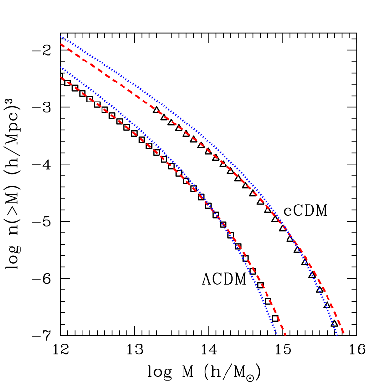
One of the challenges of calibrating systematic effects in BAO is the very large scale of the acoustic feature, which requires huge volumes to be surveyed/simulated and reduces the effects of nonlinearities and astrophysical uncertainties. While the latter is what makes BAO an attractive standard ruler, the combination makes it challenging to measure systematics with any statistical precision. To avoid these issues, we start with a toy cosmology (CDM, see also Carlson et al. (2009)) which has , , , and =1. This cosmology has an unrealistically high baryon fraction, a much smaller acoustic oscillation scale (Mpc compared with the Mpc of the ‘concordance’ cosmology) and is more nonlinear at than our Universe is believed to be. This emphasizes the effects we are investigating while reducing the sampling error, simplifying the numerical problem and allowing us to obtain highly robust measures of small effects. In § V, we extend the model constructed to concordance CDM cosmologies, focusing on one with , , , and for definiteness.
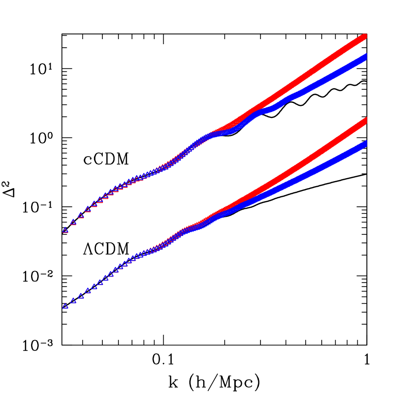
To model nonlinear structure formation and the formation of dark matter halos we used 10 independent simulations each of particles in periodic, cubical boxes of side length Gpc. The simulations were started at using the Zel’dovich approximation and evolved to with the TreePM White (2002) code. The full phase-space data were dumped at a number of redshifts between and , and groups were found using the friends-of-friends algorithm Davis et al. (1985) with a linking length of 0.168 times the mean interparticle spacing. We keep all groups down to 10 particles, or , using the sum of the particle masses in the group as our halo mass definition for simplicity. These minimum masses correspond to peak heights running from at to at . The mass function and nonlinear power spectrum for this model are shown in Figures 1 and 2 for reference. Throughout this paper we do not subtract shot-noise from the power spectra, but allow it to be a nuisance parameter in our fits (see below). More details on these simulations, including convergence tests, are in Carlson et al. (2009).
Fitting the acoustic scale involves locating the position of the acoustic feature while allowing for variations in the broad-band shape due to e.g. galaxy biasing. We do so by fitting the observed power spectra with
| (1) |
where and are smooth functions and measures the acoustic scale relative to a “best-guess” cosmology. is a template for the biased, nonlinear acoustic feature. This definition of peak “shift” is over and above the shift in the point where , or shifts in the extrema of the oscillations in the power spectrum. A good match between theory and observations, including the correct background cosmology and hence distance-redshift relation, should give .
Note that the precise partitioning into acoustic feature and broad band shape is dependent on the particular choices of and . Since constructing an accurate template for the acoustic feature yields a good template for larger scales, we assume is a constant. is assumed to be a cubic spline specified at , , , and derivatives specified at the end points. The shot noise component is simply absorbed into . The above prescription yields seven nuisance parameters; we do not vary this (or the particular prescription) in this paper, although we do get consistent results for different choices.
The fits are done by minimization, fitting the 70 power spectrum bins between and . We assume a diagonal covariance matrix where the errors are a smooth fit to the run to run variance of the 10 simulations. The errors on all derived quantities are determined the variance of 1,000 bootstrap resamplings.
We now turn to the purpose of this paper - the determination of , first for the matter and then for biased tracers.
III Matter
As is dramatically evident in Fig. 2, the sharp acoustic feature at high redshift gets smeared by bulk flows and super-cluster formation as the Universe evolves Bharadwaj (1996a, b); Meiksin et al. (1999); Eisenstein et al. (2007); Crocce and Scoccimarro (2008); Matsubara (2008a). An estimate of the smearing is given by convolving the matter correlation function with a Gaussian of width equal to the rms displacement of particles from their initial positions. To lowest order this is the rms Zel’dovich displacement
| (2) |
suggesting a template of the form
| (3) |
where is the linear theory power spectrum at the redshift of interest, and is allowed to vary. The lowest order result is the same whether obtained using the peak-background split Eisenstein et al. (2007), renormalized perturbation theory Crocce and Scoccimarro (2008) or resummed Lagrangian perturbation theory Matsubara (2008a). While the Gaussian form of the smearing is a reasonable approximation to what we see in the simulations, we find deviations from in our cosmology.
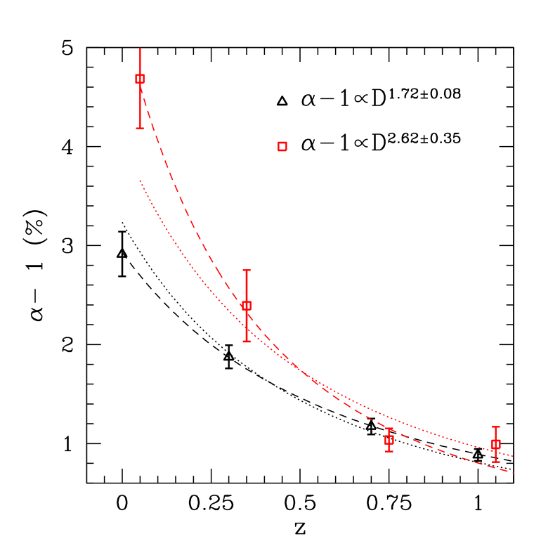
Figure 3 and Table 1 summarize the shifts obtained using the above template. We find that at very high significance, with at . We remind the reader that this is an extreme cosmology; the shifts for a concordance cosmology (as we discuss in §V) are approximately an order of magnitude smaller. We also observe that the shifts decrease with redshift as (adopting the convention ), consistent with the field getting more linear at higher redshift and suggestive that the next order terms in perturbation theory (, see Carlson et al. (2009) for a recent review) are responsible (see also Crocce and Scoccimarro (2008); Smith et al. (2008) who emphasized this point).
| DM | x | w/ | |
|---|---|---|---|
| 0.0 | |||
| 0.3 | |||
| 0.7 | |||
| 1.0 |
To explore this possibility, we expand the density contrast in powers of linear density
| (4) |
with . It is straightforward to show that
| (5) | |||||
where the contain dot products of the vectors and can be generated from recurrence relations Goroff et al. (1986); Makino et al. (1992); Jain and Bertschinger (1994). If the initial field is Gaussian the nonlinear power spectrum is then given by
| (6) |
where and . In what follows, we refer to these groups of terms as the and terms respectively. The terms also arise if we take the cross-spectrum of the initial and evolved fields, while the terms only arise in the auto-spectrum.
Ignoring combinatorial factors, the terms are given by
| (7) |
If we factor out the common and focus on the lowest order correction, , we see that it involves a integral over a single and a relatively broad kernel which suppresses the oscillations. We expect these terms not to lead to significant out-of-phase contributions, though they can contribute corrections to the damping described above. Since we can isolate these terms by considering the cross-spectrum between the initial and evolved matter fields, we can test the above hypothesis. Table 1 demonstrates that the shifts in this cross-spectrum are reduced by over an order of magnitude compared to the auto-spectrum and are consistent with zero given our statistical precision. Note that the above argument is only true for the lowest order contribution, but higher order terms are suppressed by additional factors of , and therefore drop off even more strongly with redshift.
The lowest order term is
| (8) |
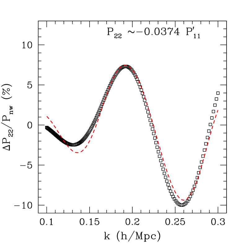
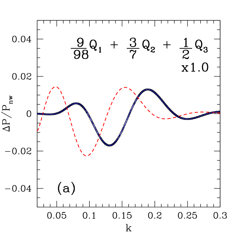
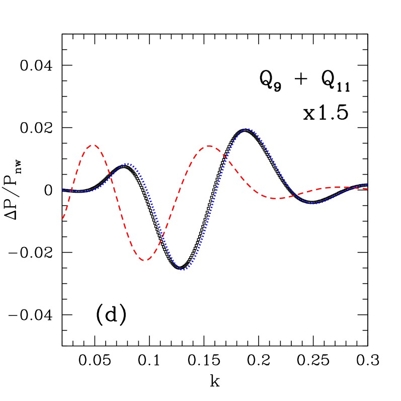
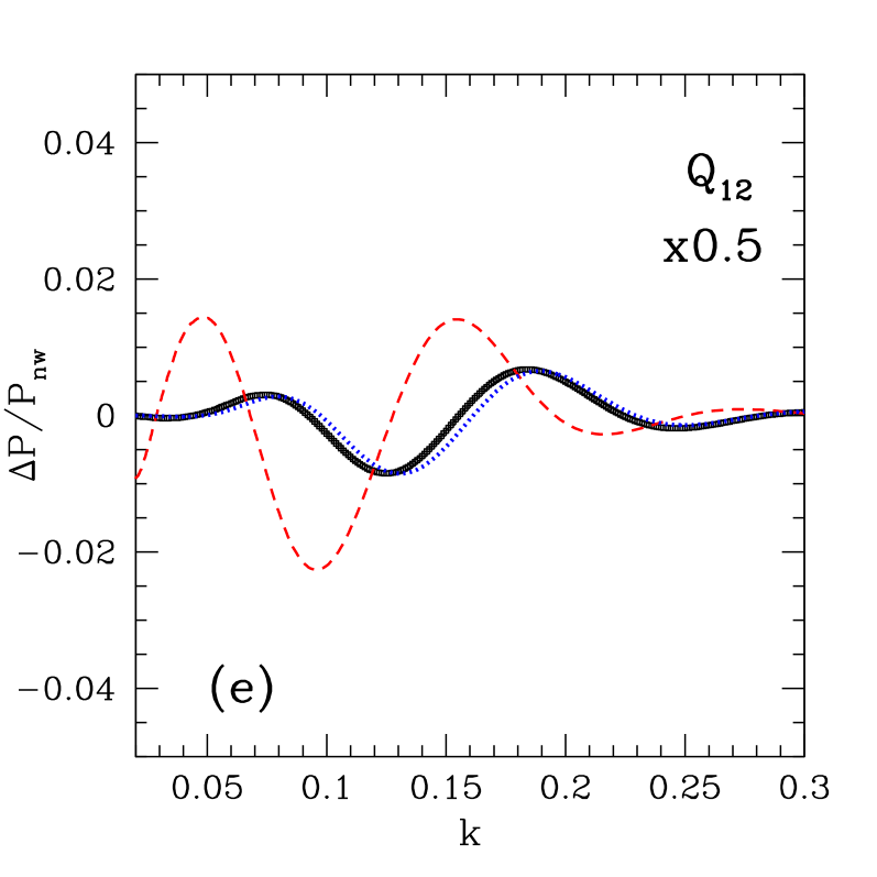
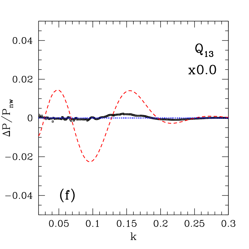
where the s are defined in Appendix A. In constrast with , these terms (see Eq. 41) involve integrals of products of which can lead to out-of-phase terms. For example, is peaked around . When contains an oscillatory piece, e.g. , contains a piece schematically of the form , which oscillates out-of-phase with . Panel (a) of Fig. 6 explicitly shows this; in fact, this oscillatory part of is very similar to scaled log-derivative of (Fig. 4; see also Crocce and Scoccimarro (2008)). Taylor expanding a shifted power spectrum,
| (9) |
we find good agreement between the predicted shift of Fig. 4 and the measured shift in Table 1. It is important to note that we have subtracted smooth components for all of these comparisons suggesting that even though perturbation theory does not accurately predict the broad-band shape Carlson et al. (2009), it does capture the evolution of the acoustic feature.
The above suggests a modified template,
| (10) | |||||
Note that we have damped the oscillations in as for although we fix the damping scale to the first order calculation. While this damping follows naturally from the heuristic picture described at the start of this section, it is also a consequence of the resummations in eg. Lagrangian perturbation theory. Table 1 shows that such a template corrects for the shifts observed in the matter.
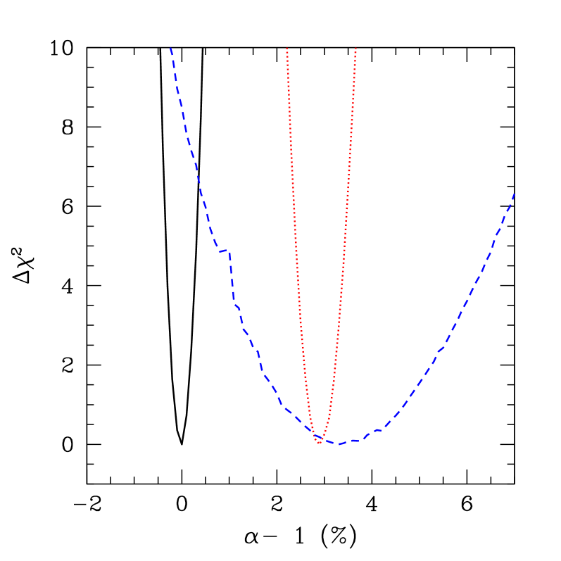
Looking ahead to biased tracers, we note that one cannot simultaneously fit for the amplitude of the term and the shift, since these are highly degenerate (Eq. 9). Doing so results in highly degraded constraints on the acoustic scale, as is evident in Fig. 5. We need to know the relative amplitude of and to correct the shift. For the mass the relative amplitude is straightforwardly given by perturbation theory. Do the same terms come in for biased tracers and are we able to determine the relative amplitude of the two types of terms?
IV Halos
IV.1 Shifts
We investigate the acoustic signal of biased tracers in our simulations by computing the clustering of samples of dark matter halos chosen to lie in narrow mass ranges. Specifically we use the linear theory power spectrum to convert from halo mass to peak height, , and pick halos in the range , , . For these we compute both the auto-power spectrum and the cross-power spectra with the linear and evolved dark matter density field. Given the low number density of most of our samples, we focus on the cross-power spectra in the analysis below.
| 1.0 | 1.3 | 1.6 | 1.9 | |
|---|---|---|---|---|
| 0.0 | ||||
| 0.3 | - | |||
| 0.7 | - | - | ||
| 1.0 | - | - | - | |
| 0.0 | ||||
| 0.3 | - | |||
| 0.7 | - | - | ||
| 1.0 | - | - | - | |
| 0.0 | ||||
| 0.3 | - | |||
| 0.7 | - | - | ||
| 1.0 | - | - | - |
Motivated by the development in the previous section, we test if analogous results exist for halos; Table 2 and Fig. 3 summarize our findings. We find that (i) the halos exhibit non-zero shifts that are functions of halo type, (ii) the shifts scale approximately as , and (iii) the shifts are once again absent in the cross-spectrum with the linear density field. As with the matter, this argues that, within the language of perturbation theory, the shifts come from terms and are dominated by second order corrections. The amplitude of the terms relative to the terms depends on the type of tracer, to which we now turn.
IV.2 Eulerian and Lagrangian Bias
We can proceed to develop the perturbation theory of biased tracers in two ways: via Eulerian or Lagrangian perturbation theory. We begin with the former and follow Fry and Gaztanaga (1993) in defining
| (11) |
Implicit here is that the halo density is defined in configuration space, and that the density fields have been smoothed on some scale to allow us to truncate the expansion. We assume that we are working on scales , and will ignore subtleties that arise from the smoothing Heavens et al. (1998); McDonald (2006) for now; we explicitly reinstate the smoothing scale in Sec. IV.3.2.
The halo auto-power spectrum in Eulerian perturbation theory becomes (see also Heavens et al. (1998); McDonald (2006); Smith et al. (2007))
| (12) | |||||
with terms like included in the missing terms denoted . The cross spectrum between two tracers and can be obtained by the replacements
| (13) |
As an example, for the cross-spectrum with the mass we obtain
| (14) |
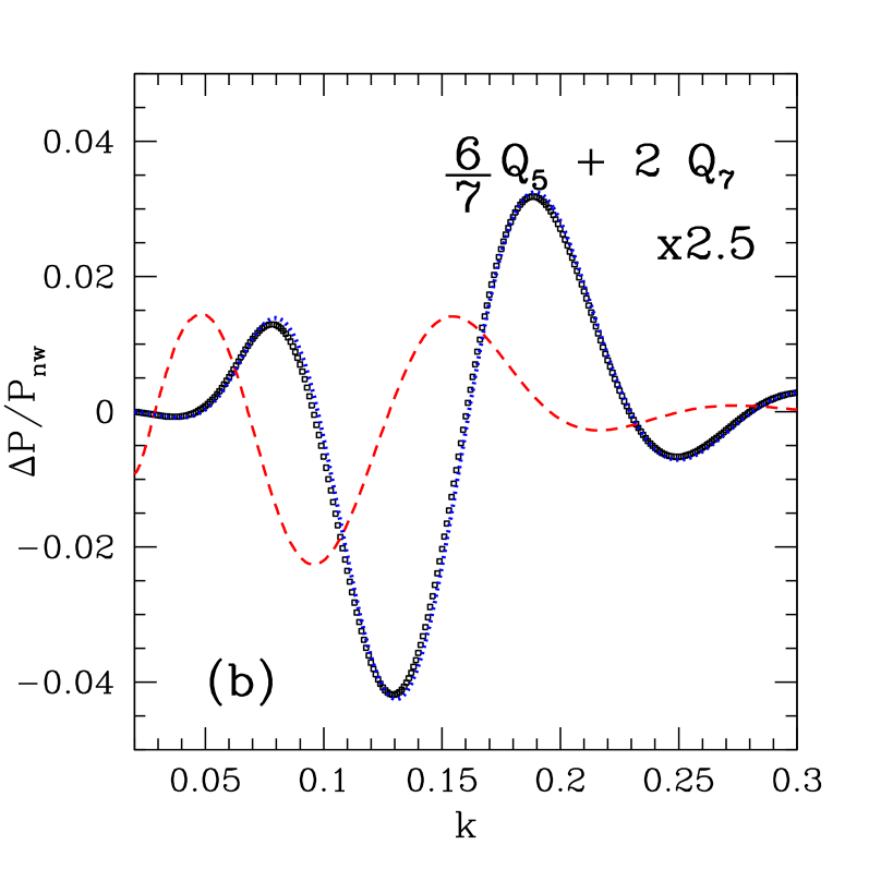
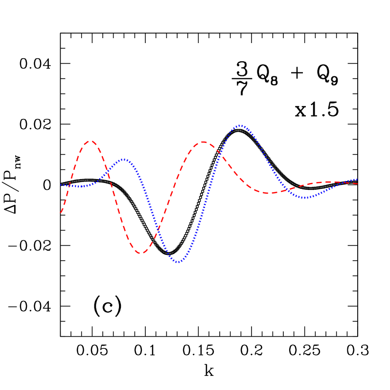
Figure 6 shows that the and terms contain out-of-phase oscillations with very similar shapes while the term is essentially non-oscillatory. This suggests that biased tracers will exhibit different shifts than the matter, and the difference will depend on the structure of the bias. It is also worth pointing out that the shift for a tracer is not the same as for the mass - a fact also evident in Table 2 where the halos exhibit different shifts from the matter!
The alternative description is within the Lagrangian picture, which has recently been developed in Matsubara (2008b) (see also Appendix B for the basic definitions). Within this formalism the halo auto-spectrum can be written
| (15) | |||||
where again terms like have been included in . As before, expressions for cross-spectra follow from the mapping in Eq. IV.2, taking care to expand the term before making the substitutions. Again, Figure 6 shows that the terms which arise look like scaled versions of , except for which is non-oscillatory.
The structure of these two sets of power spectra appears quite different, especially in the scaling of the different out-of-phase terms with . However once broad-band power is removed, both of these cases can be effectively written as
| (16) |
where we have implicitly assumed that in both cases some of the higher order terms we have neglected above would sum to an exponential damping, as happens in some variants of both Eulerian and Lagrangian perturbation theory. For the autopower spectra, using the empirically determed scalings in Figure 6, the s are related to the bias parameters by
| (17) |
or
| (18) |
Analogous expressions can be written for the cross-spectra by making the substitutions described above.
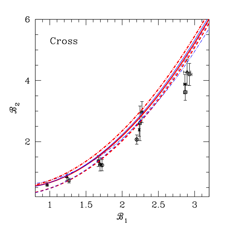
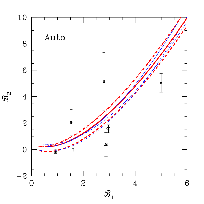
If we fit our N-body data to Eq. (16) we find that this form is a good description of the data and the different samples all lie in a narrow band in the plane, as shown in Figure 7 for both the auto- and cross-spectra. This suggests that the halos form a 1-parameter family in terms of the nonlinear bias. This is fortunate, because the ratio of to is degenerate with the shift of the acoustic scale.
IV.3 Explaining the Shifts
The previous results simply imply that the amplitude of the shifts is a function of halo bias. However, the perturbative formulation of the previous section also relates the amplitude of the shift to the bias parameters of the halos. We test this relationship here, first using the peak-background split model (see e.g. Cole and Kaiser (1989); Mo and White (1996); Sheth and Tormen (1999)) and an empirically calibrated - relationship from simulations.
IV.3.1 Peak-Background Split
The starting point for the peak-background split is the unconditional multiplicity function
| (19) |
which can be fit with
| (20) |
where , gives the Press-Schecter mass function Press and Schechter (1974), while , yields the Sheth-Tormen mass function Sheth and Tormen (1999). Within the assumption of the peak-background split, the conditional multiplicity function is given by the substitution,
| (21) |
where is the background density and is the critical overdensity for collapse. The Lagrangian bias parameters then follow from Taylor expanding the (appropriately normalized) conditional multiplicity function as a function of , yielding or
| (22) |
and
| (23) |
The Eulerian bias parameters are then defined by the mapping of the halo density from Lagrangian to Eulerian space,
| (24) |
where the factor of comes from the mapping of the Lagrangian to Eulerian volumes. Assuming that the Eulerian and Lagrangian densities may be related by the Taylor series Mo and White (1996) with assuming spherical collapse, we obtain (see also Scoccimarro et al. (2001))
| (25) |
and
| (26) |
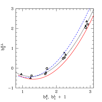
The theory then makes predictions for both the mass-halo cross-spectrum and the halo-halo auto-spectrum, with the former having significantly less shot noise. Fig. 7 compares these predictions to the observed relation between the s, where we have translated from the bias parameters using the prescription in the previous section. For the cross-spectrum the simple model describes the observed trend with , with the differences between the Press-Schecter and Sheth-Tormen predictions being small (and not distinguishable by the data). Both models overpredict at high . Interestingly, the predictions for the Eulerian and Lagrangian descriptions are virtually indistinguishable, even though the structure of the expressions for the power spectra are very different. For the auto-spectrum we have much more limited N-body data, but again the simple model does an adequate, if not perfect, job of describing what we see.
IV.3.2 An empirical relation
A second approach is to empirically calibrate and using models based upon simulations. Recall that in any survey aiming to measure BAO there will be ample data on small scales with which to construct models of the tracers.
The traditional approach to determining the Eulerian bias parameters is to compare various moments of “counts-in-cells” to the perturbative expressions. A concern with such an approach is the effective scale of the measurements, and the validity of the perturbative expressions. An alternative is to compare the auto-spectra of the halos and the mass with the cross-spectrum. The combination of the three spectra can be used to isolate and , but this tends to be very noisy and proper shot-noise subtraction is an issue. We outline a different approach below that explicitly only uses large scales; we defer detailed comparisons with other methods to future work.
We start by considering the configuration space statistic
| (27) | |||||
where and is the nonlinear matter density smoothed on a scale such that the Eq. 11 is valid. Working to second order in the density field, the second term above reduces to . If we work on large scales , then we can approximate the smooth fields by the underlying density field. Fourier transforming, we obtain
| (28) |
The limit yields a direct measure of ,
| (29) |
where
| (30) |
Note that these expressions explicitly work at large scales, where the perturbative expansion is valid. While the above derivation was for Eulerian bias, Appendix B shows that the same limit yields
| (31) |
implying that . This is a different relationship that what we obtained within the peak-background split, reflecting the different assumptions made.
The procedure for determining from our simulations are straightforward, except for one subtlety if determining from the initial particle data. Since the initial particle positions are tied to a grid, there is an excess of power at the particle Nyquist frequency, which can alias to lower frequencies when computing . To avoid this, we smooth the initial density field before squaring; this modifies to
| (32) |
where is the Fourier transform of the smoothing kernel (we adopt a Gaussian of comoving width Mpc). We then determine by fitting the measurements below to Eq. 28 where is determined from the low limit of the halo-linear density cross correlation.
Fig. 8 shows the measured bias parameters for our CDM simulations, compared with the Eulerian and Lagrangian predictions. Fig. 7 demonstrates that the observed relationship well describes the observed correlation, and therefore shifts in the acoustic scale. It is important to emphasize these constraints on are independent of the acoustic oscillations. In fact, the constraint depends on the contribution to the power spectrum, which is irrelevant for BAO.
In principle higher order measures or the observed clustering on small(er) scales contain information about for the sample of interest, and we have shown that improving our ability to model the higher order terms could bear dividends. Testing such methods is beyond our scope here, and we defer it to future work.
IV.4 Shifts, Corrected - A Template for Halos
We are now in a position to construct a template for the BAO feature traced by halos. The key ingredient is a calibrated relationship; we assume the Sheth-Tormen form of Eulerian peaks-bias here. Assuming an estimate of the large-scale bias, this fixes . We fit the observed power spectrum to
| (33) | |||||
where and are fit parameters, is determined from linear perturbation theory (Eq. 2).
We show that this procedure returns (almost) unbiased estimates of the acoustic scale in Table 2. These results come from the halo-mass cross-spectrum, which is significantly better determined than the halo auto-correlation function. The results from the auto-correlation function are consistent with the shift being corrected, but the errors are too large to allow a meaningful constraint with the simulations we have. In principle one could obtain even more accurate constraints by modeling each of the perturbation theory terms separately, but this becomes more model dependent so we don’t pursue this line here.
These results allow us to identify sources of systematic errors in the BAO measurement and estimate their level. However, before doing so, we first extend our results from CDM to CDM.
V Implications for CDM
In order to extend the results of the previous sections to a CDM cosmology, it is useful to summarize the various components of our model and see how they generalize to a different cosmology.
-
•
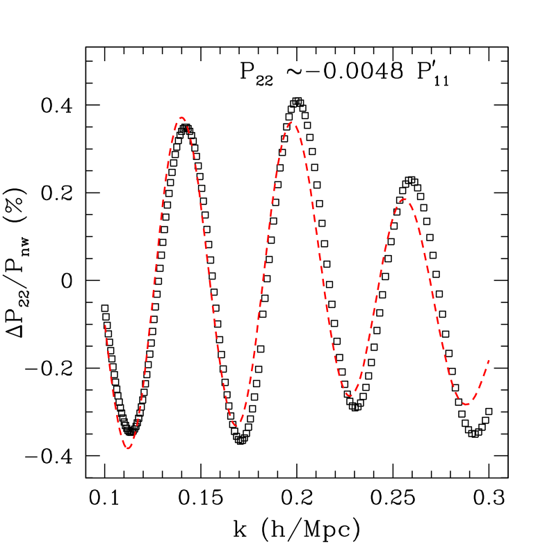
The shifts in the matter were caused by the piece of the power spectrum, which well approximated a scaled derivative of the linear power spectrum (after subtracting out the broad-band shape). The scaling was directly interpretable as the shift in the acoustic scale. Fig. 9 shows that this continues to hold for CDM, with the shift predicted to be , in agreement with simulation results by Seo et al. (2008) and analytic arguments by Crocce and Scoccimarro (2008); Taruya et al. (2009).
-
•
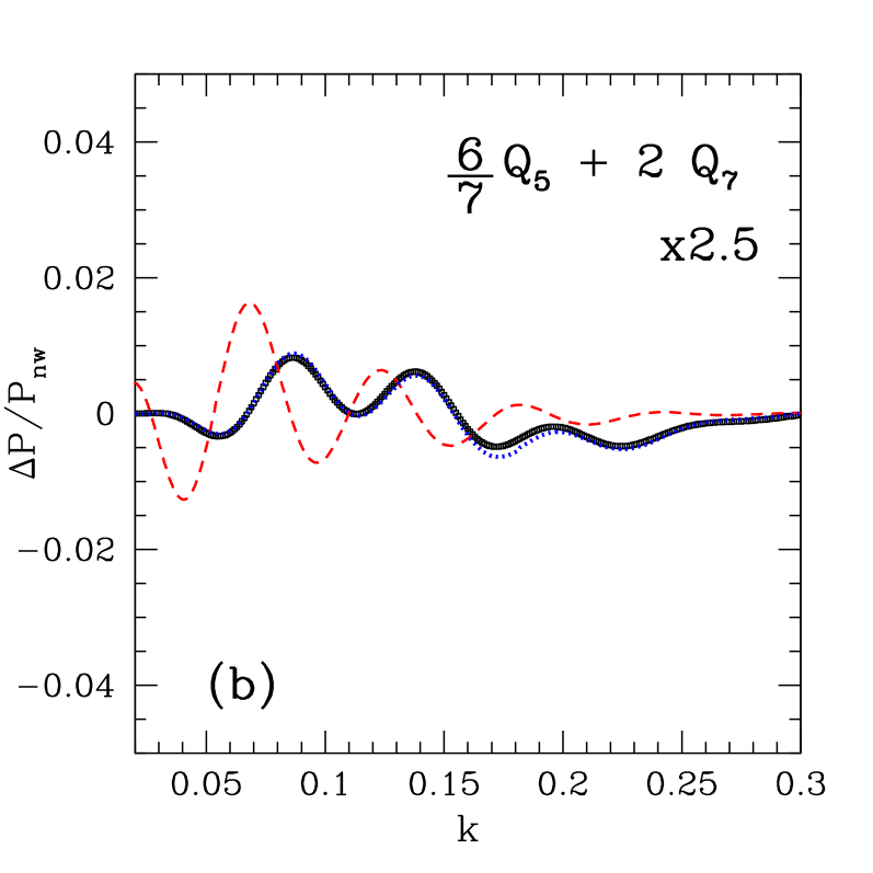
Extending these results to biased tracers generated additional shifts, sourced by terms whose oscillatory components resembled scaled versions of . This continues to be true in CDM with exactly the same scalings of ; Fig. 10 shows an example. This implies that the template of Eq. 33 as well as the relationship between the and the bias parameters continues to hold for CDM.
-
•
The final component was to demonstrate that simple models of halo bias indeed explained the resulting shifts. The first of these - a peaks-bias model - is manifestly cosmology independent. The second attempted to empirically calibrate the bias parameters; Fig. 11 shows a similar calibration for CDM. Interestingly, we find a similar cosmology independence for the empirical calibrations, manifested in both the comparisons with CDM and with the different redshifts for CDM.
-
•
The above allows us to predict that for CDM the shift is roughly an order of magnitude smaller than CDM and is given by .
We can now turn to the systematic error budget for BAO. The expression above gives the bias in the acoustic scale if one ignored the effects in this paper. Errors in the calibration of directly translate into an error in the acoustic scale; eg. a error in (approximately how good our toy models are) would correspond to a bias of .
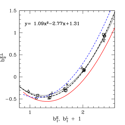
Our analysis also demonstrates that the degree of shift is sensitive to the degree of nonlinearity, or amplitude of the power spectrum. The out-of-phase terms scale as one higher power of than the linear terms. To the extent that the amplitude is degenerate with a change in bias of the tracer, uncertainty in the amplitude leads to uncertainty in the shift. As an example, if the local slope of the relation is and we imagine holding the large-scale power fixed, a change in the amplitude will induce a change and in the term in Eq. (16). From Fig. 7 we see typical values of . Applying the same scaling between and as above this would lead to a shift in the acoustic scale of for CDM. Thus knowledge of the amplitude of would give uncertainty in .
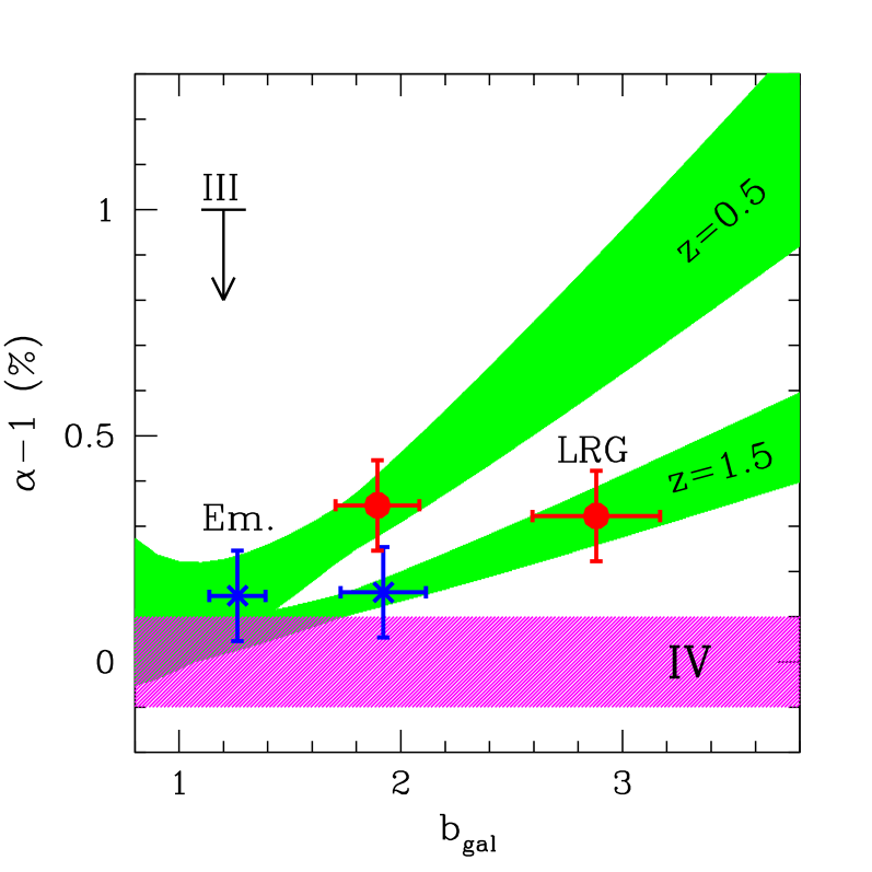
Fig. 12 summarizes the systematic error budget, and compares it to the observational error goals for Stage III and Stage IV experiments Albrecht et al. (2006). None of these systematics are expected to be relevant for Stage III experiments, and are within a factor of a few of the requirements for Stage IV experiments.
VI Galaxies
The above results have focused on the case of halo samples of a single mass, but can be generalized to arbitrary combinations of halo samples. Of particular interest is the halo model for galaxies (for a review, see Cooray and Sheth (2002)), that has been very successful in describing the large scale clustering of galaxies.
The halo model assumes that all galaxies live in dark matter halos and the probability of a particular galaxy occupying a given halo depends only on the halo mass. Under this assumption the large scale clustering of galaxies is determined by the clustering of the halos, weighted by the mean number of galaxies in each halo. If we denote the mean number of galaxies in a halo of mass as , the galaxy power spectrum is
| (34) |
where is the halo cross-spectrum for masses and and the weights are determined by the halo mass function, , and via
| (35) |
Substituting Eq. 16 for the halo power spectrum and noting that the exponential damping is (to a good approximation) independent of halo mass, we find that retains the same structure,
| (36) |
but with new coefficients
| (37) | |||||
where the normalizing factor
| (38) |
is just the mean number of galaxies. Then, assuming factorizes (or is a sum of factorizable pieces), we can simply replace in our earlier expressions with
| (39) |
Note that, as expected, simplifies to where the galaxy bias is just the weighted sum of the halo ’s. The expressions for cross-spectra of galaxy samples follow a similar pattern to the halo cross spectra discussed earlier (Eq. IV.2).
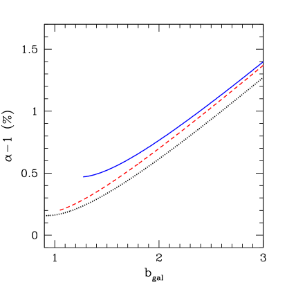
For a concrete example, we assume a of the form,
| (40) |
We consider two cases : or a “threshold” sample, and or a “satellite” sample; Fig. 13 plots the shifts as we vary from upwards. As one might expected, the increased weighting towards higher halo masses increases the shifts, although they remain smaller than the required systematics levels for near future surveys. The above also suggests that one could control systematics by re-weighting galaxies, the details of which will, of course, be population dependent.
VII Redshift space
Until now, everything we have done has been in real space, ignoring the redshift space distortions that arise from peculiar velocities. The Lagrangian perturbation theory formalism allows us to predict the effect of large-scale redshift space distortions in a straightforward manner, although the comparison with simulations is made more difficult and additional modeling of the observations is required. We defer a detailed comparison with simulations to future work, but comment on the trends here.
The power spectrum now becomes anisotropic, , with the cosine of the angle between the line-of-sight and and our previous results correspond to . Including the full dependence results in different combinations of entering the expression. Some of these are in phase with , while some are out of phase. This means the shifts in redshift space will be different than those in real space, as seen in simulations (e.g. Seo et al. (2008)). The in-phase term (, see Eq. A73 in Matsubara (2008b)) is much smaller than , and we ignore it for now.
If we concentrate on the isotropic piece of the power spectrum Padmanabhan and White (2008), we again find that the remaining combinations of which enter are proportional to and the constants of proportionality appear to cosmology independent (though they do depend additionally on ). There are no new degrees of freedom introduced theoretically, so in principle the redshift space shifts are determined from the same modeling as the real space shifts discussed previously.
For CDM at the predicted shift in the matter grows from to , consistent with the shifts seen in Seo et al. (2008). For biased tracers, the effect is to increase the shift by an -dependent (but roughly bias-independent) constant. For (corresponding to high ), this constant is , while for (corresponding to ), it is . If uncorrected, these shifts could be relevant for future experiments; we leave detailed calibrations to future work.
VIII Discussion
The propagation of acoustic waves in the early universe provides a robust means for determining the expansion history of the Universe, and contraining cosmology. The standard ruler is calibrated in the linear regime by observations of the CMB, but observed today with biased, nonlinear tracers. Since the acoustic scale is so large, the effects of bias and nonlinearity on the acoustic scale is small, but future experiments may have enough sensitivity that it needs to be taken into account. We have begun this program here.
Using a set of N-body simulations of an extreme cosmology, in which the acoustic scale is relatively small and the nonlinearity quite pronounced, we have shown that shifts in the scale grow quadratically with the amplitude of the linear theory power spectrum for both the mass and for dark matter halos. Motivated by this, and guided by arguments from Eulerian and Lagrangian perturbation theory, we found the dominant second-order contribution to the peak shift. This contribution, , quite well approximates the derivative of the acoustic signal, explaining why it leads to a peak shift and allowing us to estimate how the amplitude of the term can be translated into a shift in the fitted acoustic scale.
For dark matter halos the contribution depends on two bias parameters, and , allowing in principle arbitrary shifts of the acoustic scale. We showed however that dark matter halos, which will be the hosts of any galaxies we observe, obey a relation between and which is relatively well predicted by the peak-background split. Once these two terms are related the acoustic scale for nonlinear, biased tracers can be accurately determined, allowing high fidelity measurements of distances using baryon acoustic oscillations.
We have described how redshift space distortions affect the scale shifts within the context of Lagrangian perturbation theory, where they increase the shift by tens of percent at low and about a factor of at high .
In this paper we have concentrated on the effects of nonlinear gravitational evolution and halo biasing, showing that these effects could be understood at the level. At this level of precision the inclusion of additional physics, such as differential evolution of the baryonic and dark matter components or the details of galaxy formation, may enter and investigations in this direction should be undertaken. We have also assumed that the linear theory template is perfectly understood, which also deserves further study. Such investigations must be part of any future high-precision BAO experiment.
The simulations presented in this paper were carried out using computing resources of the National Energy Research Scientific Computing Center and the Laboratory Research Computing project at Lawrence Berkeley National Laboratory. NP is supported by NASA HST-HF-01200.01 and LBNL. MW is supported by NASA and the DoE. This research was additionally supported by the Laboratory Directed Research and Development program at Lawrence Berkeley National Laboratory, and by the Director, Office of Science, of the U.S. Department of Energy under Contract No. DE-AC02-05CH11231.
Appendix A Expressions for for
The expressions for for a biased tracer (in both Eulerian and Lagrangian perturbation theory) can be simply written by defining Matsubara (2008b)
| (41) |
where , is the linear power spectrum and the are given by
Appendix B Computing in resummed LPT
We present expressions for evaluating in resummed Lagrangian perturbation theory, where is the density field of biased tracers. These expressions follow Matsubara (2008b) and we refer the reader there for detailed calculations.
The density field for a biased tracer can be defined by the displacement field and a function of the smoothed initial density field in Lagrangian space, , as
| (42) |
where and are the Eulerian and Lagrangian positions and is the 3D Dirac function. We implicitly assume that the argument to has been smoothed on some scale much smaller than the large scales of relevance here, allowing us to ignore the smoothing here (see Matsubara (2008b) for a detailed justification). We cross correlate this with a field defined by ; is then simply obtained by taking the -th derivative with respect to and setting to zero.
The cross-power spectrum of the two fields is then given by (compare to Eq. 9 of Matsubara (2008b))
| (43) |
where and is the Fourier transform of . The correlators of interest are then given by
| (44) |
The algebra now follows through as in Matsubara (2008b) using the cumulant expansion theorem, and collecting all zero-lag correlators to yield (compare to Eq. 24 in Matsubara (2008b)),
| (45) | |||||
where
| (46) |
and
| (47) |
with denoting the connected moments.
Given Eq. 45, it is straightforward (if tedious) to compute expressions for the correlators in Eq. 44. Of particular interest to us here is the limit of which, as in Eulerian perturbation theory, is given by
| (48) |
with defined by
| (49) | |||||
While the full formalism is required in general, we note that this limit can be obtained more simply by dropping the term in Eq. 43, leaving only Gaussian fields in the exponent. These fields have only a second connected moment, thus only the term survives in the last exponential of Eq. 45 and expanding this exponential gives Eq. 48.
References
- Peebles and Yu (1970) P. J. E. Peebles and J. T. Yu, Astrophys. J. 162, 815 (1970).
- Sunyaev and Zeldovich (1970) R. A. Sunyaev and Y. B. Zeldovich, Astrophys. Space Sci. 7, 3 (1970).
- Doroshkevich et al. (1978) A. G. Doroshkevich, Y. B. Zel’Dovich, and R. A. Syunyaev, Soviet Astronomy 22, 523 (1978).
- Eisenstein and Hu (1998) D. J. Eisenstein and W. Hu, Astrophys. J. 496, 605 (1998), eprint arXiv:astro-ph/9709112.
- Meiksin et al. (1999) A. Meiksin, M. White, and J. A. Peacock, Mon. Not. R. Astron. Soc. 304, 851 (1999), eprint arXiv:astro-ph/9812214.
- Eisenstein et al. (2007) D. J. Eisenstein, H.-J. Seo, and M. White, Astrophys. J. 664, 660 (2007), eprint arXiv:astro-ph/0604361.
- Bharadwaj (1996a) S. Bharadwaj, Astrophys. J. 460, 28 (1996a), eprint arXiv:astro-ph/9511085.
- Bharadwaj (1996b) S. Bharadwaj, Astrophys. J. 472, 1 (1996b), eprint arXiv:astro-ph/9606121.
- Crocce and Scoccimarro (2008) M. Crocce and R. Scoccimarro, Phys. Rev. D 77, 023533 (2008), eprint 0704.2783.
- Matsubara (2008a) T. Matsubara, Phys. Rev. D 77, 063530 (2008a), eprint 0711.2521.
- Smith et al. (2008) R. E. Smith, R. Scoccimarro, and R. K. Sheth, Phys. Rev. D 77, 043525 (2008), eprint arXiv:astro-ph/0703620.
- Seo et al. (2008) H.-J. Seo, E. R. Siegel, D. J. Eisenstein, and M. White, Astrophys. J. accepted (2008), eprint arXiv:0805.0117.
- Padmanabhan et al. (2008) N. Padmanabhan, M. White, and J. D. Cohn, ArXiv e-prints (2008), eprint 0812.2905.
- Press and Schechter (1974) W. H. Press and P. Schechter, Astrophys. J. 187, 425 (1974).
- Sheth and Tormen (1999) R. K. Sheth and G. Tormen, Mon. Not. R. Astron. Soc. 308, 119 (1999), eprint arXiv:astro-ph/9901122.
- Carlson et al. (2009) J. Carlson, M. White, and N. Padmanabhan, ArXiv e-prints (2009), eprint 0905.0479.
- White (2002) M. White, Astrophys. J. Supp. 143, 241 (2002), eprint arXiv:astro-ph/0207185.
- Davis et al. (1985) M. Davis, G. Efstathiou, C. S. Frenk, and S. D. M. White, Astrophys. J. 292, 371 (1985).
- Goroff et al. (1986) M. H. Goroff, B. Grinstein, S.-J. Rey, and M. B. Wise, Astrophys. J. 311, 6 (1986).
- Makino et al. (1992) N. Makino, M. Sasaki, and Y. Suto, Phys. Rev. D 46, 585 (1992).
- Jain and Bertschinger (1994) B. Jain and E. Bertschinger, Astrophys. J. 431, 495 (1994), eprint arXiv:astro-ph/9311070.
- Fry and Gaztanaga (1993) J. N. Fry and E. Gaztanaga, Astrophys. J. 413, 447 (1993), eprint arXiv:astro-ph/9302009.
- Heavens et al. (1998) A. F. Heavens, S. Matarrese, and L. Verde, Mon. Not. R. Astron. Soc. 301, 797 (1998), eprint arXiv:astro-ph/9808016.
- McDonald (2006) P. McDonald, Phys. Rev. D 74, 103512 (2006), eprint arXiv:astro-ph/0609413.
- Smith et al. (2007) R. E. Smith, R. Scoccimarro, and R. K. Sheth, Phys. Rev. D 75, 063512 (2007), eprint arXiv:astro-ph/0609547.
- Matsubara (2008b) T. Matsubara, Phys. Rev. D 78, 083519 (2008b), eprint arXiv:0807.1733.
- Cole and Kaiser (1989) S. Cole and N. Kaiser, Mon. Not. R. Astron. Soc. 237, 1127 (1989).
- Mo and White (1996) H. J. Mo and S. D. M. White, Mon. Not. R. Astron. Soc. 282, 347 (1996), eprint arXiv:astro-ph/9512127.
- Scoccimarro et al. (2001) R. Scoccimarro, R. K. Sheth, L. Hui, and B. Jain, Astrophys. J. 546, 20 (2001), eprint arXiv:astro-ph/0006319.
- Taruya et al. (2009) A. Taruya, T. Nishimichi, S. Saito, and T. Hiramatsu, ArXiv e-prints (2009), eprint 0906.0507.
- Albrecht et al. (2006) A. Albrecht, G. Bernstein, R. Cahn, W. L. Freedman, J. Hewitt, W. Hu, J. Huth, M. Kamionkowski, E. W. Kolb, L. Knox, et al., ArXiv Astrophysics e-prints (2006), eprint arXiv:astro-ph/0609591.
- Cooray and Sheth (2002) A. Cooray and R. Sheth, Physics Reports 372, 1 (2002), eprint arXiv:astro-ph/0206508.
- Padmanabhan and White (2008) N. Padmanabhan and M. White, Phys. Rev. D 77, 123540 (2008), eprint 0804.0799.