Deducing the three gauge interactions
from the three Reidemeister moves
 

Abstract

Possibly the first argument for the origin of the three observed gauge groups and thus for the origin of the three non-gravitational interactions is presented. The argument is based on a proposal for the final theory that models nature at Planck scales as a collection of featureless strands that fluctuate in three dimensions. This approach models vacuum as untangled strands, particles as tangles of strands, and Planck units as crossing switches.

Modelling vacuum as untangled strands implies the field equations of general relativity, when applying an argument from 1995 to the thermodynamics of such strands. Modelling fermions as tangles of two or more strands allows to define wave functions as time-averages of oriented strand crossing density. Using an argument from 1980, this allows to deduce the Dirac equation.

When fermions are modelled as tangled strands, gauge interactions appear naturally as deformation of tangle cores. The three possible types of observable core deformations are given by the three Reidemeister moves. They naturally lead to a U(1), a broken and parity-violating SU(2), and a SU(3) gauge group. The corresponding Lagrangians also appear naturally.

The strand model is unique, is unmodifiable, is consistent with all known data, and makes numerous testable predictions, including the absence of other interactions, of grand unification, of supersymmetry and of higher dimensions. A method for calculating coupling constants seems to appear naturally.

Keywords: gauge interactions, strand model, standard model, coupling constants

PACS numbers: 12.10.-g, 12.60.Rc

1 Planck units, strands and unification

Physics as we know it today, i.e., quantum field theory and general relativity, is a low energy version of physics at the Planck scale. Effects of the Planck scale are known to be most evident on horizons, especially on black hole horizons. A basic result of twentieth-century physics is that at horizons, vacuum and particles mix. Therefore, we can guess that particles and vacuum are made of common constituents. In addition, the surface dependence of black hole entropy tells us that these constituents are not point-like, but extended.

Three questions ensue. First, what is the simplest description of nature that contains these results? Second, can the standard model of elementary particles be deduced from such a description? Third, is such a description unified? We shall argue that the answer to the first question are fluctuating featureless strands in three spatial dimensions, and that the answers to the second and third question are affirmative.

Figure 1: The simplest observation, a ‘point-like’ event in three spatial dimensions, and its associated strand model.

It is known that the observer invariance of Planck units, in particular the invariance of the maximum speed $c$, the invariance of the quantum of action $\hbar$ and the invariance of the Planck force $c^{4}/4G$, are sufficient to deduce the Dirac equation of quantum theory [Battey-Pratt & Racey 1980, Schiller 2008b] and Einstein’s field equations of general relativity [Jacobson 1995, Schiller 2005].

In contrast to a widespread opinion, a model of physics at the Planck scale therefore does not need to start from the Dirac equation or from the Einstein equations; it is sufficient to start from the invariance of the Planck units. As long as a unified model leaves the Planck units invariant for all observers, the Dirac equation and the Einstein equations are automatically satisfied.

Probably the simplest model that allows the transition from Planck units to quantum field theory and to general relativity as intuitive as possible is a model based on featureless strands. Strands, not points, are assumed to be the fundamental constituents of matter, radiation and vacuum. In other words,

$\rhd$Nature is assumed to be made of fluctuating strands in three spatial dimensions.

To describe observations, the strand model uses one new basic postulate:

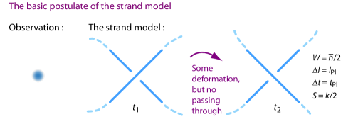
$\rhd$Each Planck unit and each event is the switch of a crossing between two strand segments.

This definition of an event as a crossing switch is illustrated in Figure 1. Every event is characterized by Planck’s quantum of action $\hbar$, the Planck time $t_{\rm Pl}=\sqrt{G\hbar/c^{5}}$, the Planck length $l_{\rm Pl}=\sqrt{G\hbar/c^{3}}$, and the Planck entropy, i.e., the Boltzmann constant $k$. More precisely, the process shown in Figure 1 corresponds to an action $\hbar/2$, while $\hbar$ corresponds to a full turn. (For any specific shape change, the number of crossing switches is observer-dependent; this is related to Lorentz and gauge transformations.) The basic postulate thus declares that events are not points on manifolds, but (observable) crossing switches of (unobservable) strands. Events are thus only point-like in the approximation that the Planck length is negligibly small.

The strands are featureless: they have no mass, no tension, no branches, no fixed length, no diameter, no ends and cannot be cut. Strands have no observable property at all: strands are unobservable. Only crossing switches are observable.

Figure 2: An example of strand deformation leading to a crossing switch.

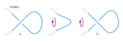
Above all, strands are impenetrable; realizing a crossing switch thus always requires the motion of strand segments around each other. A simple example of deformation leading to a crossing switch is shown in Figure 2.

Figure 3: A schematic illustration of the strand model for the vacuum.

The strand model asserts that matter, radiation and vacuum are all built from fluctuating strands. In particular,

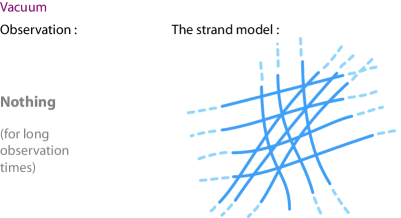
$\rhd$Vacuum is made of fluctuating unknotted and untangled strands.

Flat vacuum shows, averaged over time, no knots, no tangles and no other crossing switches, so that it is observed to be empty of matter or radiation, as illustrated in Figure 3. Independently of the strand model, in a recent exploration of the small scale structure of space-time from various different research perspectives in general relativity, Steven Carlip also comes to the conclusion that all these perspectives suggest the common idea that “space at a fixed time is thus threaded by rapidly fluctuating lines” [Carlip 2010].

$\rhd$Continuous, three-dimensional background space is introduced by the observer, in order to describe observations.

Describing nature without a background seems impossible. To be self-consistent, the background must arise, as it does here, from the time-average of the vacuum strands. In short, the strand model makes use both of discrete strands and of a continuous background. Curvature and horizons have a natural description in terms of strands; the model proposes that strands describe quantum geometry at Planck scales. Indeed, exploring the thermodynamics of strands yields the field equations of general relativity, a natural model of event horizons as strand weaves, and black hole entropy [Jacobson 1995, Schiller 2008]. Universal gravity emerges in the exactly the same way as explained recently [Verlinde 2010, Padmanabhan 2009]. These connections are not topic of the present paper, however.

Figure 4: A massive free spin 1/2 fermion built of tangled strands with its core and tails (left) and the corresponding probability cloud that results from averaging its crossing switch distribution over time (right), showing the corresponding particle position and phase.

$\rhd$Particles are tangles of strands.

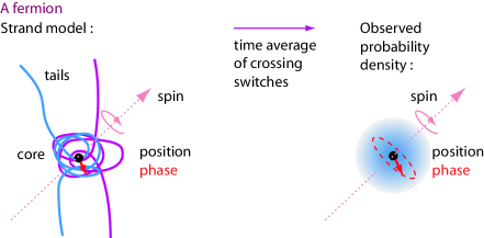
As shown below, this definition of particles can yield spin 1/2 or spin 1 behaviour for elementary particles, depending on the tangle details. In particular, tangles lead to a model of fermions illustrated in Figure 4 and Figure 5. This model of fermions is known to allow deducing the Dirac equation [Battey-Pratt & Racey 1980, Schiller 2008b]; the argument will be summarized below.

In summary, the strand model appears to make it possible to describe nature, and in particular vacuum, matter and radiation, with the help of fluctuating strands in a three-dimensional background defined by the observer. Table 1 lists the main correspondences between physical systems and tangles. In all physical systems, the shape fluctuations of tangles lead to crossing switches and thus, indirectly, to the usual evolution of matter, radiation and vacuum curvature. Crossing switches are used to define the fundamental physical units, and thus all physical observables.

Before even exploring the physical consequences, two issues arise: (1) Where do fluctuations come from? (2) What is their influence on the dynamics? The strand model argues that strand fluctuations arise automatically, whenever a continuous, three-dimensional background space-time is introduced by the observer, and that the fluctuations of a particular piece of strand are due to all other pieces of strands in the universe. The model also argues that the fluctuations have precisely the behaviour that allows introducing a background: the fluctuations are homogeneous and isotropic. In particular, whenever two strands approach each other, the fluctuations of the two strands become correlated due to their impenetrability, but the embedding in a three-dimensional background remains possible (on a local scale). Whenever a background can be introduced (i.e., whenever fluctuations are, on average, locally homogeneous and isotropic), Einstein’s field equations and Dirac’s equation are not sensitive to any assumed detailed properties or dynamics of the fluctuations, as long as the fluctuations lead to the usual space-time symmetries [Schiller 2008, Schiller 2008b].

Table 1: Correspondences between physical systems and mathematical tangles.

Physical system	Strands	Tangle type
Vacuum and dark energy	many infinite unknotted strands	unlinked
Elementary vector boson (radiation)	one infinite strand	trivial or knotted curve
Elementary fermion (matter)	two or three infinite strands	braided, rational or prime tangle
Graviton	two infinite twisted strands	rational tangle
Gravity wave	many infinite twisted strands	many rational tangles
Horizon	many woven infinite strands	weave-like tangle

1.1 Appearance and unification of interactions

We will argue that the definition of an event as a crossing switch of strands yields a model for the three gauge interactions. A separate discussion specifies the tangle structure for each elementary particle [Schiller 2009]. For the following discussion, we assume flat space-time.

To show the natural appearance of exactly three gauge interactions from the basic postulate, we will use three older results and a new one:

(1) tangles of strands allow to define wave functions and reproduce the Dirac equation [Battey-Pratt & Racey 1980, Schiller 2008b],

(2) shape deformations are equivalent to gauge theory [Berry 1984, Wilczek & Zee 1984, Putterman & Raz 2008],

(3) all observable tangle deformations can be reduced to only three types [Reidemeister 1926, Kauffman 1991].

As we will see, these three results allow to deduce the U(1) and the broken SU(2) gauge symmetries, including the corresponding Lagrangians. With the new result that

(4) the group SU(3) appears in an expanded belt trick with three belts,

also the strong interaction Lagrangian is recovered.

We thus aim to deduce the main aspects of the Lagrangian of the standard model from strands. To do this, we first recall briefly how the Dirac equation for free, non-interacting, elementary spin 1/2 particles and its Lagrangian are deduced. We start with the spin aspects.

1.2 Spin and statistics

Figure 5: The belt trick or scissor trick or string trick: rotations by 4 $\pi$ of an object with three or more tails are equivalent to no rotation – allowing a suspended object, such as a belt buckle or a tangle core, to rotate for ever. Note that there are two ways to perform the belt trick after a rotation by 4 $\pi$ is completed, as is best illustrated by an internet animation [Egan 2009].

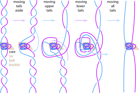
It is known since many decades that so-called belt trick – also called scissor trick or string trick – illustrated in Figure 5, can be used, together with its variations, to model spin 1/2 behaviour. It is also well-known that fluctuating strands with tails reaching the ‘border’ of space reproduce the spin-statistics theorem for bosons and fermions, depending on the tangle details [Schiller 2008b].

The belt trick implies that for fermions made of two or more tangled strands, and thus with four or more tails to the ‘border’, as shown in Figure 4 and Figure 5, a rotation by $4\pi$ of the tangle core – thus a rotation by two full turns – brings back such a tangle to the original state. In short, the belt trick allows a object that is attached by strands to spatial infinity to rotate indefinitely. The same is valid for a tangle core.

In addition, after exchanging two tangle cores twice, tail fluctuations alone can return the situation to the original state. Cores made of two or more tangled strands thus behave both under rotations and under exchange like spin 1/2 particles.

For cores made of one strand – thus with two tails to the border – a rotation by $2\pi$ restores the original state. Such a core, shown in Figure 6, behaves like a spin 1 particle, thus like a boson.

Figure 6: A massive spin 1 boson in the strand model (left) and the observed probability density when averaging its crossing switches over long time scales (right).

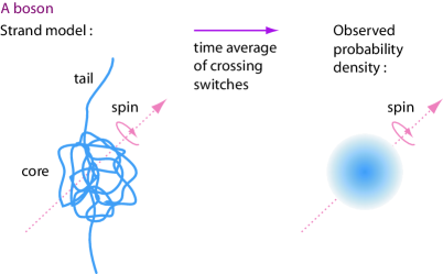
As shown in Figure 3, in the strand model, the vacuum is modelled as a collection of untangled strands. A strand model for the graviton, invariant under rotations by $\pi$ and thus with spin 2, has been introduced in the discussion of general relativity [Schiller 2008].

In short, the spin-statistics connection for all elementary particles can be reproduced by the strand model. All evolution and all particle reactions conserve spin, because all interactions conserve the number of strands and tails, as will be detailed below. The strand model also implies that spin values are always an integer multiple of 1/2. In summary, the strand model reproduces spin in all its observed details [Schiller 2008b]. In particular, tangles of two or more strands reproduce spin 1/2 particles.

1.3 Wave functions for fermions

Figure 7: The definition of a crossing, its position and its orientation.

We now summarize the definition of wave functions using strands. Given a fluctuating tangle of several strands, we define:

$\rhd$The wave function of a system described by a tangle is the time average of the positions and the orientations of its crossings (and thus not of its crossing switches).

Each crossing of two strand segments in a three-dimensional background defines a line of shortest distance, as shown schematically in Figure 7. The centre of this line defines a position and an orientation for each crossing. For the definition of the wave function, the time average of crossing positions and orientations is taken over the typical time resolution of the observer. This is a time interval that is much longer than the Planck time, but also much shorter than the typical evolution time of the system. The time resolution is what the observer calls an ‘instant’ of time. Typically, the resolution will be ${10^{-25}}$ ${\mathrm{s}}$ or longer; the typical averaging will thus be over all times between ${10^{-43}}$ ${\mathrm{s}}$, the Planck time, and ${10^{-25}}$ ${\mathrm{s}}$ or more.

The wave function can thus be called the ‘oriented crossing density’. As such, it is a continuous function of space. The wave function thus captures the local time average of all possible tangle fluctuations. For a tangle with a few crossings, Figure 4 illustrates the idea. However, the figure does not show the wave function itself, but its probability density. In fact, the probability density is the (square root of the) crossing position density, whereas the wave function is a density that describes both position and orientation of crossings. The strand model thus visualizes the idea of wave function with an oriented cloud. We also mention that the Hilbert structure is easily deduced from the strand definition of wave functions [Schiller 2008b].

For particles with spin 1/2, not only the time-average of crossing density is a function of space; also the time-average of the spin axis orientation is. One scalar, $\rho(x,t)$, is needed to describe the crossing density, and three Euler angles, $\alpha$, $\beta$ and $\gamma$, are needed to describe the axis orientation. As a result, the natural description of a tangle that includes the orientation of the axis is by two complex numbers that depend on space and time

$$\Psi(x,t)=\sqrt{\rho}{\rm e}^{\alpha/2}\left(\begin{array}[]{{c}}\cos(\beta/2){\rm e}^{i\gamma/2}\\ i\sin(\beta/2){\rm e}^{-i\gamma/2}\end{array}\right)\;,\;$$ (1)

which is the natural description of the non-relativistic wave function. Due to the belt trick, the expression only contains half angles. And due to the half angles, the two-component wave function is a spinor [Schiller 2008b]. This is the strand basis of the two-component wave function that is used in the Pauli equation since over half a century [Bohm & al. 1955].

In the relativistic case, four additional functions of space are needed to describe the wave function. One additional function, a phase, describes with what probability the time-averaged local belt-trick is performed left-handedly or right-handedly. Three additional functions describe the relativistic boost parameters (or, if preferred, three additional Euler angles). In total, this doubles the functions used in the Pauli equation.

In total, the strand model requires 8 real functions of space to describe the local wave function of spin 1/2 particles, of which 1 behaves like a density and 7 behave like phases. These 8 real functions can be organized as 4 complex functions of space and form what is usually called a Dirac spinor [Baylis & al. 2007].

In summary, the strand model describes wave functions as time-averaged oriented crossing densities. Or shorter: wave functions are blurred tangles.

1.4 Dirac’s equation

Already a long time ago [Battey-Pratt & Racey 1980] it was shown that the belt trick implies the Dirac equation. Battey-Pratt and Racey deduced this result by exploring a rotating object connected by strands (tails) to spatial infinity, in the way shown in Figure 5. In their approach, the rotating object plus the (unobservable) tails would correspond to a microscopic particle. (In the strand model, the central object becomes the tangle core.) An object that is continuously rotating is described by a phase; Battey-Pratt and Racey could show that this phase obeys the Dirac equation for free particles, if antiparticles are added.

A simple way to see the equivalence, though different from the argument by Battey-Pratt and Racey, is the following. We imagine that the tails are not observable, that the central object is negligibly small, and that it defines the position of the microscopic particle. In this case, a continuous rotation of the central object corresponds to Feynman’s rotating little arrow in his well-known popular book on QED [Feynman 1988]. Because of the tails, the central object obeys spinor statistics and spinor rotation behaviour, as we saw above. Thus the tails, despite being unobservable, lead to the typical interference behaviour of a spin 1/2 particle. In other words, the path integral description of quantum theory follows directly from Battey-Pratt and Racey’s approach.

In the strand model, the central object is simply the tangle core, and it is assumed that its effective size, when tightened, is of the order of a few Planck lengths, which makes elementary particles point-like for all practical purposes. Using tangles and crossing switches for the derivation of the Dirac equation also has the advantage to introduce $\hbar$ in a natural way.

In other words, the Dirac equation results from fluctuating tangles. The Dirac equation describes how time-averaged fluctuating tangles evolve over time. In particular, antiparticles are tangles rotating in the opposite direction, and $C$, $P$ and $T$ transformations can be modelled in terms of strands [Battey-Pratt & Racey 1980, Schiller 2008b].

In other terms, both Battey-Pratt and Racey and the strand model state that the free Dirac equation arises naturally when looking for a description of the belt trick that is valid for infinitesimally small angles. In the past, the relation between the belt trick and the free Dirac equation has been a curiosity without physical consequences. However, we now argue that the belt trick for interacting tangles can be used to deduce the three known gauge groups. To see this connection, we first recall the relation between strands and Lagrangians.

1.5 Lagrangians and the principle of least action

What we call action in physics is, in the strand model, the number of crossing switches. Action is thus measured in multiples of $\hbar/2$.

In the strand model, all observed motion is due to one or several crossing switches – which themselves are due to change of tangle shape, induced by strand fluctuations. In the strand model, quantum states are time-averaged tangle shapes. A specific average tangle shape represents a specific quantum state.

Evolution changes quantum states, and thus tangle shape averages. Given that strands are fluctuating entities, and thus that all observed motion is due to strand fluctuations, we expect that the simplest evolution, i.e., the evolution that requires the smallest number of crossing switches, will be the most favoured one. The evolution with the smallest number of crossing switches is the evolution with the smallest action. In short, the least action principle is a natural outcome of the strand model. (In fact, the minimization of crossing switch number leads directly to Schwinger’s quantum action principle [Schwinger 2001]; this is an alternative way to deduce quantum theory from the strand model.)

Energy is action per time. Therefore, in the strand model, energy is the number of crossing switches per time. Kinetic energy $T$ is, in the strand model, the number of crossing switches per time induced by shape fluctuations of tangle cores. Potential energy $U$ is the number of crossing switches per time induced by external fields; as we will see shortly, fields are modelled by strand loops that induce crossing switches when they approach tangle cores.

The Lagrangian density is the total number of crossing switches per volume and time, averaged over many Planck scales. This means that the textbook definition of the free matter Lagrangian in terms of wave functions (and their complex conjugates) and the definition of the free radiation Lagrangians in terms of radiation fields (squared) appears naturally in the strand model [Schiller 2008c]. The Lagrangian densities of a free fermion,

$${L}_{\mathrm{Dirac}}=\bar{\psi}(i\hbar c\displaystyle{\not}\partial-mc^{2})\psi$$ (2)

and of the free electromagnetic field

$${L}_{\mathrm{Maxwell}}=-\frac{1}{4\mu_{0}}F_{\mu\nu}F^{\mu\nu}$$ (3)

are thus a direct consequence of the strand model.

Special relativity is also reproduced by the strand model. In the strand model, the invariant limit speed $c$ in nature is given by the (most probable) speed of a single, helically deformed, massless, i.e., unknotted strand. The definition of the action

$$S=\int Ldt\;,\;$$ (4)

together with the averaging procedure based on the space-time background defined by the observer, automatically makes the action a Lorentz invariant.

In summary, it is possible to derive Dirac’s equations and the Lagrangians for free particles from the basic postulate of the strand model, and the principle of least action is the statement that physical systems evolve with as few crossing switches as possible. The detailed description underlying this short summary has been given elsewhere [Schiller 2008b].

1.6 Gauge interactions and core deformations

The above introduction summarized how the deformation of tangle tails is related to spin behaviour and Lorentz invariance. In short, tail deformations induce space-time symmetries. We will now show that, in contrast, core deformations induce gauge symmetries, using the following relations:

$\rhd$In the strand model, gauge interactions are modelled by the various deformations of tangle cores induced by external (radiation) fields. These deformations transfer crossings between boson and fermion tangles.

$\rhd$In the strand model, gauge invariance of matter (and radiation) fields is modelled by the invariance of tangle cores (and boson tangles) under changes of definition of phase.

We will show in the following that there are three different ways to deform tangle cores and to redefine core phases. These three ways lead to exactly three gauge interactions – and to no other.

2 The QED Lagrangian – U(1) gauge interaction

Figure 8: Twists are core deformations whose group has a single generator; certain tangles are affected and other are not affected by twists, when averaged over long time scales; and random twists generate Coulomb’s inverse square law.

Figure 9: How the set of generalized twists – the set of all local rotations of a single strand segment around an axis – forms a U(1) group group.

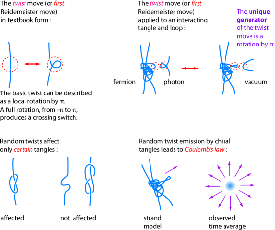
In the strand model, any observable deformation must switch some crossings. The simplest way to deform a tangle core, while changing its crossing number at the same time, is to take a piece of strand and to twist it. This is shown in Figure 8. In knot theory, this type of deformation is called the first Reidemeister move. We will soon find out that the addition of a twist to a core – or better, the transfer of a twist between a core and a single external strand – has the same properties as what is usually called the emission or absorption of a photon.

We note that a twist transfer from a loop to a core – as shown on the top right of Figure 8 – does not imply any cutting of strands. An approaching twisted loop will influence the fluctuations of the core, due to strand impenetrability, and will lead to an effective transfer of twist, without any ‘ugly’ change of topology.

A twist has the same effect on a tangle core as a local rotation by an angle $\pi$. The set of all local rotations, for any angle, forms a U(1) group. We thus conjecture that twists represent the electromagnetic interaction.

We note that large numbers of random twists will affect certain tangle cores while they will not affect others, as shown in the bottom left of Figure 8. For example, if we take a single, knotted strand, we expect that its long-time average motion will be affected by random twists only if the knot is chiral. In other words, knotted chiral strands represent electrically charged bosons, whereas knotted achiral strands represent neutral bosons.

In summary, sensitivity to twists suggests to define electric charge with the chirality of a particle tangle. For example, a granny knot represents one elementary charge. Right and left chirality then correspond to positive and negative charge. As a consequence of this definition, charge values for free particles are naturally quantized. (A separate discussion [Schiller 2009] shows how the definition of charge is extended to quarks and to doubly charged hadrons.)

Because all interactions are only strand deformations – in particular, strand interpenetration being forbidden – total tangle chirality is conserved in all interactions. In short, the strand model predicts that electric charge is conserved in all interactions, as is indeed observed.

The strand model states that only tangles with localized cores can be charged; only tangles with cores can be grabbed in such a way as to be twisted. In the strand model, knotted cores imply non-vanishing mass. In other words, only massive particles can be charged, exactly as is observed. In short, any charged fermion is a chiral tangle that is made of two or more strands.

Figure 10: A tangle candidate for a photon (left) and for a chiral lepton (right).

Photons are helical strands. Photons have no knotted core: they are massless and neutral. Photons come in two versions: with positive and negative helicity. Virtual photons correspond to the two types of twists that can be added to tangle cores [Schiller 2008c]. Photons cannot disappear in the strand model. The energy and angular momentum content of the helix is conserved. If one strand loses its helix, a neighbouring strand will gain it. In the strand model, photons are thus particles with infinite lifetime.

The particle tangle of the photon and a tangle of a charged fermion are shown in Figure 10. We note that despite their simple structure, photons cannot disappear. This becomes clear once the vacuum strands around the photon are drawn [Schiller 2008c].

To explore the translational motion of a fermion tangle, we remember that vacuum itself is also made of strands. To move through space, a fermion must move through the vacuum web of strands. Fermion tangles move through space either by exchanging strands with the vacuum, or by ‘passing around’ vacuum strands at spatial infinity. In short, the vacuum web hinders fermion motion; in contrast, photon motion is not hindered by the vacuum web. In short, charged (and massive) tangles are predicted to move more slowly than light, as is observed. In the strand model, the speed of light thus cannot be attained by fermion tangles: it is a limit speed.

In the strand model, the physical action of a process measures the number of required crossing switches; each crossing switch makes a contribution of $\hbar/2$. For a charged fermion in an electromagnetic field, the action will be given by three terms: the crossing switches due to the motion of the fermion, those due to the motion of the electromagnetic field, and those due to the interaction.

In the strand model, like in quantum field theory, the form of the electromagnetic interaction term is fixed by gauge invariance.

Table 2: The correspondence between shape change of tangles and gauge theory

Concept	Gauge theory	Strand model
System	Matter & gauge field	Tangle core & approaching loop
Interaction	Phase change by field	Core deformation by loop
Gauge freedom	Freedom to define quantum phase and vector potential	Freedom to define core phase and boson energy-momentum density
Gauge transformation	Changes definition of quantum phase and vector potential	Changes phase value of core and loop energy-momentum density
Gauge-dependent	Quantum phase,	Core’s angular orientation,
quantities	vector potential,	loop energy-momentum density,
	change of vector potential along open path	orientation change along an open path in (core) deformation space
Gauge-independent	Field strength,	Crossing density and flow,
quantities	phase difference along a closed path,	core phase difference after closed path in deformation space,
	integral of vector potential along a closed path	loop energy-momentum density along closed path
Gauge boson	Gauge group generator	Deformation generator
Gauge group origin	Unknown	Due to possible core deformations, classified by Reidemeister moves
Gauge groups	U(1)	Twisting a core strand
	SU(2)	Poking a core strand under another
	SU(3)	Sliding a strand across two others
Charge	Couples matter to field:	Topological property that yields:
	– electric charge	– preferred sensitivity to one sign of twist: chirality
	– weak charge	– preferred sensitivity to one sign of poke: tangledness with helicity
	– colour charge	– preferred sensitivity to one sign of slide: rationality
Coupling strength	Coupling constant	Probability of core deformation

2.1 U(1) gauge invariance

Figure 11: Various ways of defining a tangle orientation, showing the explicit U(1) gauge freedom for one such definition.

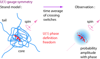
In 1984, Berry, Wilczek, Zee and Shapere deduced a well-known result about the motion of deformable bodies: the freedom to define a measure of deformation leads to a gauge theory [Berry 1984, Wilczek & Zee 1984, Putterman & Raz 2008]. The main points of this equivalence are summarized in Table 2. In particular, the studies showed that the freedom of defining a measure of deformation is analogous to the freedom of choosing a gauge. As in gauge theory, also in the study of body deformations there are gauge-dependent and gauge-independent quantities. In particular, if a sequence of deformations returns a system back to its original state, this process allows to define a quantity that is independent of the chosen deformation measure, and thus gauge-independent.

In the strand model, interactions are transfers of observable deformations, i.e., of crossing switches, between boson and fermion cores. In particular, twists change the phase of the fermion core, as shown in Figure 8. Twists can be concatenated; and they have a single generator. When concatenated twists reach a total core rotation by $4\pi$, the system can fluctuate back to its initial state. Twists thus generate a U(1) group. The corresponding gauge-invariant quantity is the number of turns of the core, in short, the phase difference.

On the other hand, the absolute phase of a tangle core is not uniquely defined. For example, the absolute phase could be defined by the direction formed by the outermost crossing with respect to the core centre. But any other direction along a circle perpendicular to the rotation axis is also possible, as shown in Figure 11. The freedom in the definition of the phase again corresponds, once the axis is given, to a U(1) group.

The other important gauge-independent quantities in this system are the volume density and the flow density of twists; this is precisely the electromagnetic field intensity, and that Maxwell’s equations follow from the twist density and flow in the macroscopic limit [Schiller 2008c]. In particular, Coulomb’s law is a consequence of the random emission, by charged fermions, of twisted loops into all directions of space. This is illustrated in Figure 8. In particular, particles of one handedness prefer to emit virtual photons of one handedness. As a result, particles of the same handedness repel, and particles of different handedness attract.

We thus recover several well-known properties of charged quantum particles: (1) electromagnetic fields change particle phase, (2) only phase differences, but not absolute phase values, can be measured, (3) charged particles move slower than light and attractor repel, and (4) there is a U(1) gauge invariance for transfers of twists, i.e., minimal coupling holds.

2.2 Quantum electrodynamics

Figure 8 shows the transfer of twists between bosons and fermions that results from the mutual hindrance of strand fluctuations. The figure also shows that random (virtual) twist emission leads, after averaging over space and time, to Coulomb’s law. Charge conservation, Coulomb’s law and its generalization for relativistic observers leads to Maxwell’s equations. In short, by averaging twist numbers over space and time we obtain the Lagrangian of the free electromagnetic field [Schiller 2008c]

$${L}_{\mathrm{Maxwell}}=-\frac{1}{4\mu_{0}}F_{\mu\nu}F^{\mu\nu}\;.$$ (5)

In addition, the U(1) gauge invariance of twist exchange between charged fermions adds an interaction term to the free Dirac Lagrangian found above. We thus get the complete Lagrangian of QED from strands

$${L}_{\mathrm{QED}}=\bar{\psi}(i\hbar c\displaystyle{\not}D-mc^{2})\psi-\frac{1}{4\mu_{0}}F_{\mu\nu}F^{\mu\nu}\;,\;$$ (6)

where $\displaystyle{\not}D$ is the U(1) gauge-covariant derivative describing the electromagnetic interaction.

Another way to see this result is the following. Our discussion showed that if we identify core twists with the electromagnetic interaction, we can deduce the following statements:

– electric charge is conserved and quantized;

– electric charges move slower than light;

– all motion is described by the quantum of action $\hbar$;

– photons are massless;

– charges emit and absorb virtual photons;

– electromagnetic fields change the phase of charged particles;

– the QED Lagrangian has a U(1) gauge symmetry.

When these statements are added to the free field Lagrangian, we get the full Lagrangian of QED.

Figure 12: The fundamental Feynman diagram for QED for a specific time orientation (left) and one of the corresponding strand diagrams (right), with different magnification scales.

Figure 13: A few QED processes described in terms of strands.

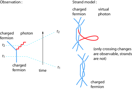
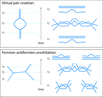
We can check the equivalence between QED and the strand model in many ways. It is well-known that all of quantum electrodynamics follows from its fundamental Feynman diagram, shown on the left of Figure 12. The strand model provides a corresponding diagram, shown on the right of the figure. (For clarity, the magnification scales are chosen differently.) On this basis, strand diagrams for all known QED Feynman diagrams can be constructed; two examples are shown in Figure 13.

We can check the equivalence of strand deformations and Feynman graphs also through their conservation properties. A twist conserves tangle topology. Therefore every twist, i.e., every electromagnetic reaction, is predicted to conserve the spin of the involved particle, and the total spin of the system. Since unchanging topology also implies unchanging flavour (as we will see below) the strand model predicts that the electromagnetic interaction conserves particle flavour. Both properties agree with observation.

Another quantity of interest is intrinsic parity $P$. Parity is related to the behaviour of tangles under reflection. In the strand model, parity $P$ is a topological quantity that distinguishes a fermion from an antifermion. The strand model automatically implies that fermions and antifermions have opposite intrinsic parity, as is observed. The strand model also predicts that photons and their ‘antiparticles’ have the same intrinsic parity, as they can be deformed into each other. This is indeed observed. Since twists conserve topology, the strand model predicts that parity is conserved in electromagnetic reactions, as is indeed observed.

Charge conjugation parity or $C$-parity is the behaviour of tangles under charge conjugation. In the strand model, charge conjugation is the exchange of all crossings [Schiller 2008b]. The strand model thus implies that only neutral particles can have a defined $C$-parity value, as is observed. The strand model also predicts that the photon tangle has negative $C$-parity, as observed. Finally, the strand model predicts that the electromagnetic interaction conserves $C$-parity for the same reason that it conserves $P$-parity. This is also observed.

2.3 Renormalization of QED

In quantum field theory, Lagrangians must not only be Lorentz and gauge invariant, but must also be renormalizable. The strand model makes several statements on this issue. At this point, we focus on QED only; the other gauge interactions will be treated below. First fo all, the strand model reproduces the observation that only one basic Feynman diagram exists for QED. In other words, the strand model of QED is equivalent to usual QED, and thus is renormalizable. The strand model thus only provides a new underlying picture for Feynman diagrams; the strand model does not change the physical results at any experimentally accessible energy scale. In particular, the measured running of the fine structure constant and of the masses of charged particles are reproduced by the strand model, because Feynman diagrams of all orders are reproduced.

The twist deformations underlying the strand model for QED suggest new ways to calculate effects of higher order Feynman diagrams, such as needed in calculations of g-factors of charged particles. In particular, the strand model for QED, as shown in Figure 12, suggests that higher order QED diagrams are simple deformations of lower order diagrams. Taking statistical averages of strand deformations thus in principle allows to calculate QED effects to arbitrary order in the coupling. However, this topic is not part of the present paper.

The strand model also suggests that the difference between renormalized and unrenormalized quantities reflects the difference between minimal and non-minimal crossing switch numbers, or equivalently, between simple and more complex, small-size tangle deformations. In more detail, unrenormalized quantities can be imagined as those deduced when the tangles are pulled tight, whereas renormalized quantities are those deduced for particles surrounded by many large-size fluctuations.

2.4 Predicted limit values and deviations from QED

The equivalence of QED Feynman diagrams and strand diagrams implies that deviations of the strand model from QED are expected only when short-time fluctuation averaging is not applicable any more; this happens only when quantum gravity starts to play a role. This will only happen near the Planck energy $\sqrt{\hbar c^{5}/4G}$.

The strand model predicts that all Planck units are limit values. For example, in the same way that the maximum speed is $c$, also the maximum elementary particle energy is the Planck energy and the shortest measurable length is the Planck length $\sqrt{4G\hbar/c^{3}}$. This view yields a maximum electric field value $E_{\rm max}={c^{4}}/{4Ge}\approx{2.4\cdot 10^{61}}\,{\rm V/m}$ and a maximum magnetic field value $B_{\rm max}={c^{3}}/{4Ge}\approx 8\cdot 10^{52}\,\rm T$ [Schiller 2008c]. All physical systems – including all astrophysical objects such a gamma ray bursters or quasars – are predicted to conform to this limit. These limit values form another way to characterize the domain where deviations of the strand model from ordinary QED are expected.

All limit values for observations have a simple explanation: limit values appear when strands are as closely packed as possible. In the strand model, strands cannot be packed more closely than to Planck distances.

In summary, the strand model suggests that U(1) invariance is valid for all energies below the Planck energy; no other gauge group at higher energy is predicted to appear, and grand unification is ruled out.

3 The weak interaction Lagrangian – broken SU(2) gauge invariance

Figure 14: Pokes as core deformations, as elements of a SU(2) group, and some tangles that are affected and some that are not affected by pokes.

Figure 15: Poke transfer is the basis of the weak interaction in the strand model. No strand is cut or reglued; the transfer occurs only through the excluded volume due to the impenetrability of strands.

Figure 16: How the set of all pokes – the set of all deformations induced on tangle cores by the weak interaction – forms an SU(2) gauge group. The relation to the belt trick, with a pointed buckle and two belts, is also shown.

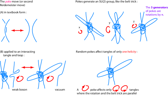
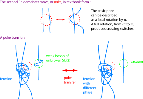
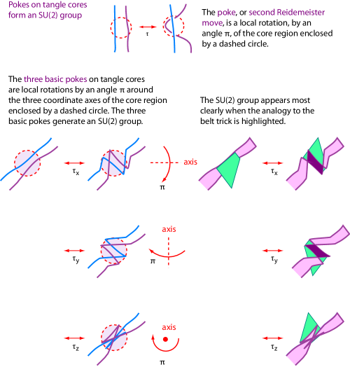
The next simplest way to deform a tangle core in such a way that the crossing number changes is to poke a piece of strand over a second piece of strand, as shown in Figure 15. In knot theory, this type of deformation is called the second Reidemeister move. We will find out that the poke deformation of a core represents what is usually called the emission or absorption of a weak vector boson.

A poke has the same effect as a localized, partial rotation (plus a possible size extension) of the tangle core. The simplest way to see this is to imagine a large number of pokes acting all over a tangle core: the core will be rotated (and possibly extended). Below, we will explore the exact conditions for this to happen.

Pokes can be concatenated and form a group. In particular, the three pokes around the three orthogonal axes, shown in Figure 16, do not commute. Closer inspection shows that the three pokes are equivalent to the operations involved in the belt trick; the commutator of two orthogonal pokes is the third poke (multiplied by $-1$ or $+1$ depending on the permutation). In addition, performing the same poke twice, we get a twisted situation; in the strand model this is represented by a $-1$ [Schiller 2008c]. The generators thus obey

$$\begin{array}[]{c|ccc}\cdot&\tau_{x}&\tau_{y}&\tau_{z}\\ \hline\cr\tau_{x}&-1&i\tau_{z}&-i\tau_{y}\\ \tau_{y}&-i\tau_{z}&-1&i\tau_{x}\\ \tau_{z}&i\tau_{y}&-i\tau_{x}&-1\\ \end{array}$$

and the group formed by pokes is thus SU(2). We thus conjecture that deformations by pokes represent the weak interaction.

As a note, it is worth recalling that the (broken, as we will see) SU(2) gauge symmetry of the weak interaction is realized in the strand model by the deformation of the tangle cores, whereas the (unbroken) SU(2) group due to the Pauli matrices due to spin 1/2 is realized through deformations of the tangle tails, keeping the core rigid. The two structures are independent.

The properties of pokes and their SU(2) gauge group differ from the U(1) twists in four aspects: they can change topology, they violate parity, they interact among themselves and they break the SU(2) symmetry.

3.1 Particle transmutation and topology change

If a poke that is applied to a fermion tangle involves spatial infinity (thus if a loop goes ‘over’ a tail at spatial infinity) the move can change the topology of the fermion. In the strand model, a different tangle topology means a different particle. There is nothing preventing this process at spatial infinity, as background space is not defined there. In short, the strand model predicts that weak interactions can transform different particles into each other. This is observed, e.g., in beta decay. In contrast, the electromagnetic twists discussed above never have this effect.

We note that the properties of pokes imply that despite particle transmutation, they conserve total electric charge, spin, and weak charge, as is observed.

3.2 Parity violation and weak charge

Certain tangle cores will be affected by large numbers of similar pokes, whereas others will not be. For example, if we take a single, knotted strand, we see that it will be rotated. In other words, single knotted strands, or massive bosons, are weakly charged. We will find out shortly that this means that the W and the Z, in contrast to photons, interact among themselves.

Let us explore a fermion tangle, in this case a rotating tangle core made of two strands – as shown in the bottom right of Figure 14 – that is subject to a large number of similar pokes. We first recall that for a given rotation by $4\pi$, the belt trick can be performed in two ways, parallel and antiparallel to the sense of rotation. (An animation showing the two options in a clear way is available on the internet [Egan 2009].) On average, a poke will act in one way on states where rotation and belt trick sense are parallel, and will act in another way – namely not at all – on states where rotation and belt trick sense are antiparallel. We thus find that fermions are affected by pokes depending on their their helicity. Antiparticles, which are represented by tangles rotating backwards, will only be affected by those pokes which do not affect particles. In short, only tangles of one handedness are weakly charged; tangles of the other handedness have no weak charge. Pokes thus reproduce the observed maximal parity violation of the weak interaction.

We note that weak charge – the weak isospin – requires localization of a tangle. In other words, the strand model predicts that only massive fermions can interact weakly, as is observed.

We also note that the ability to interact weakly does not depend on the detailed tangle topology, but only on tangledness. All fermions of a given handedness have the same weak charge (i.e., the same value for the third component of the weak isospin). The strand model thus predicts that all left-handed matter fermions (respectively, all right-handed antifermions) have the same value of the weak isospin (respectively, the same negative value), as is observed.

$C$-parity violation by the weak interaction pokes appears in the same way as $P$-parity violation. In contrast, electromagnetic twists do not violate either $P$ or $C$-parity. (The observation of a small $CP$ violation by the weak interaction is discussed elsewhere [Schiller 2009].)

3.3 Massive gauge bosons

The third difference between SU(2) pokes and U(1) twists concerns the associated gauge bosons. If we apply pokes that involve spatial infinity to the high-energy boson tangle, we get two candidates for the low energy tangles of the W and Z bosons, shown in Figure 17. Their tangles consist of a single knotted strand: they are thus massive. The chiral trefoil tangle represents the charged W boson, its mirror version the corresponding antiparticle of opposite charge; the achiral figure-eight tangle represents the Z boson. (More complex tangles of one strand represent states of even shorter lifetime with added virtual W or Z particles.)

The mass of the weak vector bosons is an essential property; it explains the weakness of the weak interactions. Since the tangles for the W and the Z are different, the strand model also reproduces their difference in mass.

Figure 17: Virtual, high-energy, unbroken SU(2) boson tangles (left) and real, low-energy W and Z boson tangles that break SU(2) (right). Poke-inducing strands (left) differ from weak vector bosons (right) because of symmetry breaking. The figure shows only the simplest possible tangles for each weak gauge boson.

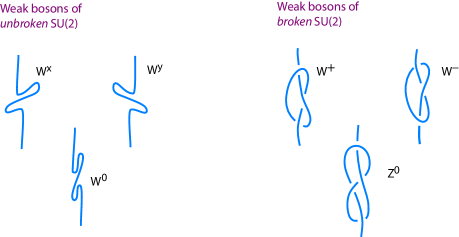
The trefoil tangle of the $W$ has spin 1; it is chiral, thus is electrically charged. It is knotted, thus has non-zero mass. The tangle has no $P$ and $C$ parity, as is observed. The figure-eight tangle of the $\rm Z$ has spin 1; it is not chiral, thus is electrically neutral. It is knotted, thus has non-zero mass. The tangle is its own antiparticle, as is observed. The tangledness of the W and Z tangles also implies that they couple to pokes, thus to themselves. The two tangles thus have non-vanishing weak isospin and lead to a non-Abelian gauge theory, a Yang-Mills theory, for the exchange of pokes.

3.4 SU(2) breaking and mass generation

The $\rm Z$, the $\rm W^{+}$ and the $\rm W^{-}$ bosons can be seen as a broken weak isospin triplet representation of the SU(2) gauge group of the weak interaction. The degeneracy is explicitly broken in the strand model: the differences in shape – e.g., in crossing numbers – of the two tangles are the reason for the symmetry breaking.

Figure 14 illustrates the weak interaction with the help of small-amplitude poke moves. In other words, the moves shown in that figure correspond to fluctuations at very high energy. At such energies, the SU(2) gauge symmetry is predicted to be exact, or unbroken, by the strand model. (This explicitly contradicts grand unified theories, which predict higher symmetry groups at high energy.)

At low energy, the pokes show effects due to the involvement of spatial infinity: at low energy, topology changes due to such poke moves thus play a role. This difference between high and low energy, the breaking of SU(2) symmetry, is illustrated in Figure 17. Knotted tangles are massive, and different knots have different masses. Thus the strand model predicts massive bosons and the breaking of SU(2) symmetry at low energy.

In other terms, the strand model predicts that a W or a Z boson is described by a large number of tangles: a tangle without a knot, a tangle with a simple knot, and an infinite number of tangles with more complex knots. In addition, the strand model predicts that tangles with (on average) more complex knots are more massive that tangles with simpler knots. This explains why the neutral Z boson is heavier than the charged W boson.

In summary, the strand model predicts that mass is a result of tangledness, and that mass generation (for bosons and for fermions) is related to the weak interaction.

3.5 QFT of the weak nuclear interaction

We can summarize the equivalence between pokes and the weak interaction in the following statements:

– weak charge is conserved, related to handedness and is defined for tangles;

– the weak charge is the same for all elementary fermions;

– the weak charge is different for bosons;

– the weak interaction violates $P$ and $C$ parity maximally;

– the weak intermediate vector bosons have mass;

– the weak interaction has a SU(2) gauge symmetry that is broken at low energy;

– weak charges emit and absorb virtual intermediate vector bosons.

All these statements, together with the Dirac equation, reproduce many terms of the electroweak Lagrangian. In particular, the SU(2) gauge invariance defines the interaction terms between the weak fermionic doublets and the weak interaction bosons.

Several terms and aspects of the electroweak interaction Lagrangian are not yet reproduced: (1) the terms involving the Higgs, (2) the quark and neutrino mixing matrices, (3) the number of generations, (4) the particle masses. These aspects are discussed elsewhere [Schiller 2009].

Figure 18: All the Feynman diagrams for the weak interaction that do not involve the Higgs field.

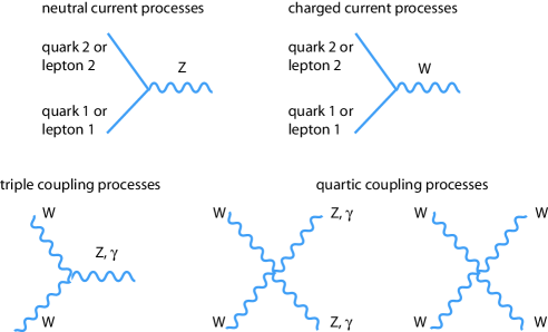
But those parts of the electroweak Lagrangian that are reproduced so far can be checked further. At energies lower than the electroweak unification scale, reactions due to the weak interaction can be classified into neutral and charged current processes, as well as triple and quartic boson couplings. This is shown in Figure 18. To describe these processes in the strand model, we need the tangles of the real and virtual intermediate vector bosons $\rm W$ and $\rm Z$ from Figure 17. The resulting strand model for neutral currents is shown in Figure 19.

Figure 19: The Feynman diagram for a weak neutral current interaction (left) and the corresponding strand diagram (right).

Figure 20: The Feynman diagram for a weak charged current interaction (left) and the corresponding strand diagram (right).

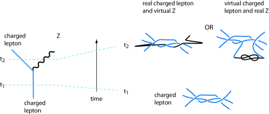
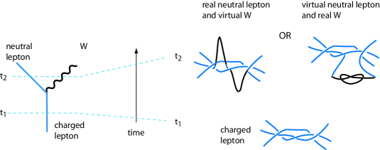
The neutral currents can be reduced to two Feynman diagrams: a leptonic vertex and a hadronic vertex, as shown in the upper left corner of Figure 18. In the strand model, leptonic neutral currents leave the topology of the interacting matter particles unchanged. In this way, weak neutral currents are automatically flavour-conserving in the strand model, as is observed.

Figure 20 for the charged currents requires a move that involves spatial infinity and then changes the topology of the involved fermions. However, the process only changes leptons into leptons and quarks into quarks, as is observed. (Hadronic neutral and charged currents, and tangles for all leptons, quarks and the Higgs boson, are discussed elsewhere [Schiller 2009].)

Figure 21: Some ternary and quartic boson couplings in the weak interaction.

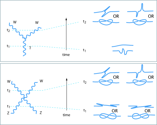
Some ternary and quartic couplings among the vector bosons are shown in Figure 21. The strand model reproduces these processes.

In all these weak strand reactions, total electrical charge, total weak isospin, baryon number and total spin are conserved, as is indeed observed. In this way, the tangle model for fermions reproduces the weak interaction, provided that the $\rm Z$ and $\rm W$ bosons are each made of one knotted strand.

3.6 Renormalization of the weak interaction

The strand model with its limited number of strands that appear in elementary particle reactions, together with the equivalence of pokes and the weak interaction, implies that only triple and quadruple vertices are possible; higher order vertices are impossible in the strand model. This is the central requirement for the renormalization of the theory. The strand model also reproduces the experimentally verified terms of the electroweak Lagrangian. (Quark and fermion mixing, as well as the Higgs boson, are discussed elsewhere [Schiller 2009].) The strand model thus automatically ensures that the electroweak interaction is renormalizable. In particular, the running of the weak coupling constant and of the masses of particles are reproduced.

3.7 Deviations from the standard model

The strand model suggests that there are no deviations from the quantum field theory of the electroweak interaction for any experimentally accessible energy. Only when gravity is of importance, the strand model predicts a maximum electroweak field, given by the Planck value. Neutron stars, quarks stars, gamma ray bursters, quasars and all other astrophysical phenomena are predicted to have field values below the limit value. So far, no observed value violates the predicted limit.

The strand model might deviate form the electroweak interaction only at Planck scales. No other gauge group comes into play even at highest energies. In particular, the strand model predicts the absence of larger gauge groups, such as those as conjectured by grand unification.

4 The strong interaction and its SU(3) gauge group

Figure 22: Slides as tangle deformations, a tangle that is affected by slides, and some tangles that are not.

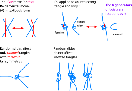
The third way to deform a tangle core while changing crossing numbers is to slide a piece of strand over a crossing of two other pieces, as shown in Figure 22. In knot theory, this type of deformation is called the third Reidemeister move. We will see shortly that the slide deformation of a tangle is related to what is usually called the emission or absorption of a gluon.

Certain tangle cores will be affected by large numbers of random slides whereas others will not be. For example, if we take a single, knotted strand, we see that it will be unaffected. In other words, single knotted strands do not interact strongly; indeed, the W and the Z are observed to be ‘white’ in the terminology of the colour force. Also the unknotted photon is predicted to be ‘white’ and thus to transform under a singlet representation. The same happens for all fermions that are prime tangles of three strands: the strand model predicts [Schiller 2009] that leptons do not interact strongly, as indeed is observed.

In fact, only few tangles are affected by large numbers of random slides. The tangle given in the lower left of Figure 22, with 4 tails, is an example. We note that in this case, the 4-tailed tangle of Figure 22 transforms as a triplet representation. (Thus we can call each of the three possible options ‘coloured’.) In fact, elementary tangle cores with mass that transform following other – e.g., faithful – representations of SU(3) are impossible. In other words, the strand model states that the photon and all massive elementary particles are either singlet (‘neutral’) or triplet (‘coloured’) representations of SU(3), as is observed.

4.1 Gluons, SU(3) and QCD

Figure 23: A single gluon strand changes the rotation of a tangle: slide transfer is the basis of the strong interaction in the strand model. No strand is cut or reglued; the transfer occurs only through the excluded volume due to the impenetrability of strands.

Figure 24: The strand deformations for the eight gluons $\lambda_{1}$ to $\lambda_{8}$ associated to the slide move, and the SU(3) structure of the strong interaction as the result of three joined belts.

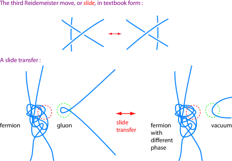
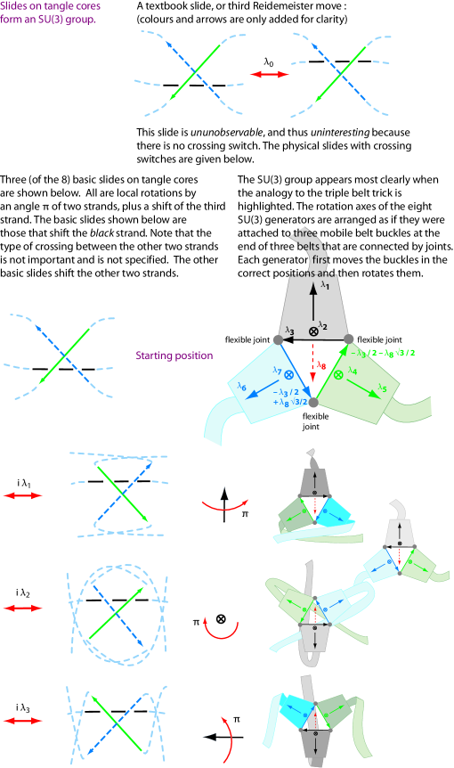
The third Reidemeister move involves three pieces of strands; the move deforms a tangle core by sliding a crossing over or under a third strand, as shown in Figure 23. In three dimensions, this operation can be realized in several ways, called $\lambda_{0}$ to $\lambda_{3}$ and shown in Figure 24. The ‘naive’ slide $\lambda_{0}$ involves no crossing switch and is thus unobservable in the strand model. The slides $\lambda_{1}$, $\lambda_{2}$ and $\lambda_{3}$ involve combined rotations by $\pi$ of two strands, thus involve crossing switches, and therefore are physical. We note that ‘slide’ is not a good term for these operations; in fact, they are combinations of a rotation by $\pi$ and a flattening into the observation plane. Nevertheless, we will continue to call them ‘slides’ for brevity.

We can find a visualization of SU(3) if we imagine three belts whose buckles are attached at joints, as illustrated in Figure 24. Three slides are attached to each buckle, thus leading to 9 slides in total. (The slides corresponding to $\lambda_{1}$ are usually called $\lambda_{5}$ and $\lambda_{6}$, those to $\lambda_{2}$ are called $\lambda_{4}$ and $\lambda_{7}$.) Three of the slides constructed in this way are linearly dependent, namely those formed by $\lambda_{3}$ and its two ‘cousins’; among them, only two are needed (called $\lambda_{3}$ and $\lambda_{8}$ in the Gell-Mann set), giving a total of 8 slides. The slides $\lambda_{1}$, $\lambda_{2}$ and $\lambda_{3}$ form an SU(2) subgroup, and the same happens on the other buckles. This models the three linearly independent SU(2) subgroups contained in SU(3).

The definition of the 8 slides allows them to be concatenated. To explore concatenations, a few details are important. First, the slides of Figure 24 correspond to $i$ times the Gell-Mann generators. Second, the slide $\lambda_{8}$ that makes $\lambda_{9}$ unnecessary is orthogonal to $\lambda_{3}$. Third, the triplet $\lambda_{1}$, $\lambda_{2}$, $\lambda_{3}$ forms a SU(2) subgroup, as does the triplet $\lambda_{5}$, $\lambda_{4}$, $-\lambda_{3}/2-\lambda_{8}\sqrt{3}/2$ and the triplet $\lambda_{6}$, $\lambda_{7}$, $-\lambda_{3}/2+\lambda_{8}\sqrt{3}/2$. Fourth, all slides are combinations of rotations and flattenings. For this reason, their square is not $-1$, but involves $\lambda_{8}$ and/or $\lambda_{3}$. Fifth, multiplying slides is concatenation, whereas adding slides is an operation defined in [Schiller 2008b]. Loosely speaking, addition connects partial tangles without additional crossings.

The multiplication table is:

$$\begin{array}[]{|c||c|c|c||c|c||c|c|c|}\hline\cr\cdot&\lambda_{1}&\lambda_{2}&\lambda_{3}&\lambda_{4}&\lambda_{5}&\lambda_{6}&\lambda_{7}&\lambda_{8}\\ \hline\cr\hline\cr\lambda_{1}&2/3&i\lambda_{3}&-i\lambda_{2}&i\lambda_{7}/2&-i\lambda_{6}/2&i\lambda_{5}/2&-i\lambda_{4}/2&\\ &+\lambda_{8}/\sqrt{3}&&&+\lambda_{6}/2&+\lambda_{7}/2&+\lambda_{4}/2&+\lambda_{5}/2&+\lambda_{1}/\sqrt{3}\\ \hline\cr\lambda_{2}&-i\lambda_{3}&2/3&i\lambda_{1}&i\lambda_{6}/2&i\lambda_{7}/2&-i\lambda_{4}/2&-i\lambda_{5}/2&\\ &&+\lambda_{8}/\sqrt{3}&&-\lambda_{7}/2&+\lambda_{6}/2&+\lambda_{5}/2&-\lambda_{4}/2&+\lambda_{2}/\sqrt{3}\\ \hline\cr\lambda_{3}&i\lambda_{2}&-i\lambda_{1}&2/3&i\lambda_{5}/2&-i\lambda_{4}/2&-i\lambda_{7}/2&i\lambda_{6}/2&\\ &&&+\lambda_{8}/\sqrt{3}&+\lambda_{4}/2&+\lambda_{5}/2&-\lambda_{6}/2&-\lambda_{7}/2&+\lambda_{3}/\sqrt{3}\\ \hline\cr\hline\cr\lambda_{4}&-i\lambda_{7}/2&-i\lambda_{6}/2&-i\lambda_{5}/2&2/3+\lambda_{3}/2&i\lambda_{3}/2&i\lambda_{2}/2&i\lambda_{1}/2&-i\sqrt{3}\lambda_{5}/2\\ &+\lambda_{6}/2&-\lambda_{7}/2&+\lambda_{4}/2&-\lambda_{8}/2\sqrt{3}&+i\sqrt{3}\lambda_{8}/2&+\lambda_{1}/2&-\lambda_{2}/2&-\lambda_{4}/2\sqrt{3}\\ \hline\cr\lambda_{5}&i\lambda_{6}/2&-i\lambda_{7}/2&i\lambda_{4}/2&-i\lambda_{3}/2&2/3+\lambda_{3}/2&-i\lambda_{1}/2&i\lambda_{2}/2&i\sqrt{3}\lambda_{4}/2\\ &+\lambda_{7}/2&+\lambda_{6}/2&+\lambda_{5}/2&-i\sqrt{3}\lambda_{8}/2&-\lambda_{8}/2\sqrt{3}&+\lambda_{2}/2&+\lambda_{1}/2&-\lambda_{5}/2\sqrt{3}\\ \hline\cr\hline\cr\lambda_{6}&-i\lambda_{5}/2&i\lambda_{4}/2&i\lambda_{7}/2&-i\lambda_{2}/2&i\lambda_{1}/2&2/3-\lambda_{3}/2&-i\lambda_{3}/2&-i\sqrt{3}\lambda_{7}/2\\ &+\lambda_{4}/2&+\lambda_{5}/2&-\lambda_{6}/2&+\lambda_{1}/2&+\lambda_{2}/2&-\lambda_{8}/2\sqrt{3}&+i\sqrt{3}\lambda_{8}/2&-\lambda_{6}/2\sqrt{3}\\ \hline\cr\lambda_{7}&i\lambda_{4}/2&i\lambda_{5}/2&-i\lambda_{6}/2&-i\lambda_{1}/2&-i\lambda_{2}/2&i\lambda_{3}/2&2/3-2\lambda_{3}&i\sqrt{3}\lambda_{6}/2\\ &+\lambda_{5}/2&-\lambda_{4}/2&-\lambda_{7}/2&-\lambda_{2}/2&+\lambda_{1}/2&-i\sqrt{3}\lambda_{8}/2&-\lambda_{8}/2\sqrt{3}&-\lambda_{7}/2\sqrt{3}\\ \hline\cr\lambda_{8}&&&&i\sqrt{3}\lambda_{5}/2&-i\sqrt{3}\lambda_{4}/2&i\sqrt{3}\lambda_{7}/2&-i\sqrt{3}\lambda_{6}/2&2/3\\ &+\lambda_{1}/\sqrt{3}&+\lambda_{2}/\sqrt{3}&+\lambda_{3}/\sqrt{3}&-\lambda_{4}/2\sqrt{3}&-\lambda_{5}/2\sqrt{3}&-\lambda_{6}/2\sqrt{3}&-\lambda_{7}/2\sqrt{3}&-\lambda_{8}/\sqrt{3}\\ \hline\cr\end{array}$$

This table is precisely that of the Gell-Mann matrices, which form a standard set of generators of the group SU(3). We thus conclude that the eight linearly independent generalized slides that can be applied to a tangle represent virtual gluons that act on a particle.

The slide analogy for virtual gluons implies that real gluons are described by single unknotted strands that impart ‘slides’ to fermions. A simple image is to describe real gluons as loops that ‘pull’ one strand during the slide, as shown in Figure 25. This single strand model also reproduces the vanishing mass of gluons and their spin 1 value.

The 8 gluons transform according to the adjoint (and faithful) representation of SU(3). The model for gluons implies that two interacting gluons can yield either one or two gluons, but not more, as shown in Figure 26. Since in the strand model, gluons do not change topology, but only shapes, gluons are predicted to be massless, despite interacting among themselves. In total, after averaging over space and time, we thus get the usual free gluon Lagrangian

$${L}_{\mathrm{gluons}}=-\frac{1}{4}G^{g}{}_{\mu\nu}G_{g}{}^{\mu\nu}$$ (7)

from the strand model.

A structure made of two or three gluons would not be knotted or linked. It is unclear whether such a structure is stable in the strand model, though appearance seems to speak against the idea. Therefore it seems that glueballs might not exist. Despite this apparent lack of a mass gap, the lack of classical gluonic waves is explained by the triple and quartic gluon vertices.

In the strand model, ‘colour’ is the name give to the property distinguishing the three states forming triplet representations. Simple visual inspection shows that slides, and thus gluons, conserve colour.

Figure 25: The strand model for the nine gluons, the last three not being linearly independent.

Figure 26: The self-interaction of gluons in the strand model.

Figure 27: The Feynman diagram of the strong interaction for a quark.

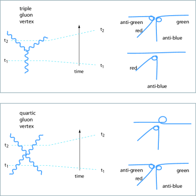
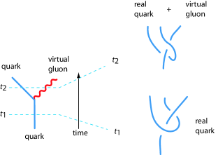
Slides, i.e., gluon emission or absorption, never change the topology of tangles. Thus the strand model predicts that the strong interactions conserve electric charge, baryon number, weak isospin, flavour, spin and all parities. This is indeed observed. In particular, there is a natural lack of $CP$ violation by slides. This is exactly what is observed about the strong interaction. The strand model thus also reproduces the lack of $CP$ violation by the strong interaction.

In short, in the strand model, the emission or absorption of a virtual gluon by a quark is expected to be a rearrangement of the strand or tails of a rational tangle, as shown in Figure 27. The specific tangles for all quarks and hadrons, with the resulting properties, are discussed elsewhere [Schiller 2009].

Starting from the idea that tangle core deformations lead to phase redefinitions, we have thus found that generalized slides imply an SU(3) invariance. In other words we find that the complete strong interaction Lagrangian density for matter and radiation fields is SU(3) gauge invariant. After averaging crossings over space and time we thus get the well-known Lagrangian

$${L}_{\mathrm{QCD}}=\sum_{q}\bar{\psi}_{q}(i\hbar c\displaystyle{\not}D-m_{q}c^{2})\psi_{q}-\frac{1}{4}G^{g}{}_{\mu\nu}G_{g}{}^{\mu\nu}$$ (8)

where $\displaystyle{\not}D$ is now the SU(3) gauge-covariant derivative. In short: the strand model reproduces QCD. Only the number of quarks, the values of their masses, and the coupling strength remains open.

4.2 Quark confinement

In the strand model, rational tangles represent quarks. Rational tangles are topologically unstable; thus they are not localizable and the do not behave like or represent free particles. In this way, the strand model explains the lack of free quarks. The strand model also explains the lack of quark decay, as explained elsewhere [Schiller 2009].

In the strand model, a bond between two quarks is a structure that connects the tails of the quarks. The simplest case is that of mesons, where a quark bonds to an antiquark. In this case, three strands form the bond between the quark and the antiquark, thus realizing something similar to the original ‘hadronic string model’. Since the resulting effective potential in mesons is confined to a tube, the strand model reproduces Regge trajectories, their common slope, mass sequences, quantum numbers, flavour oscillations, and all other properties of mesons. Also baryons are modelled successfully. More details and comparisons with experimental data are given elsewhere [Schiller 2009].

4.3 Renormalization of the strong interaction

The strand model, together with the slide move, implies that only a limited number of Feynman diagrams appear in strong nuclear reactions. In particular, the slide move implies that only one QCD Feynman diagram exists for quarks, and that only triple and quadruple vertices exist for gluons. This limited range of options is essential for the renormalization of QCD and allowed to deduce the QCD Lagrangian. The strand model thus ensures that the strong interaction is renormalizable.

The strand model provides a new underlying picture for the Feynman diagrams of the strong interaction, but does not change the physical results at any energy scale accessible in the laboratory. In particular, the running of the strong coupling constant is reproduced. (In the strand model, a flux-tube–like bond between the quarks appears automatically [Schiller 2009]. At high kinetic energies, the bond has little effect, so that quarks behave more like free particles. The strand model thus reproduces asymptotic freedom.)

4.4 Deviations of the strand model from QCD

The strand model thus seems to reproduce QCD in its essential aspects: gauge symmetry of the Lagrangian, asymptotic freedom, and quark confinement. Deviations from QCD are thus only expected near the Planck scale, when the spatial and temporal averaging of crossing switches is not possible. Again, the Planck value for the gluon field intensity is predicted to be the highest possible field value. Neutron stars, quark stars and all other astrophysical objects are predicted to have field values below this limit. This is observed. In short, deviations of the strand model from QCD are not expected for any laboratory energy.

On the other hand, the strand model implies that no other gauge group other than SU(3) comes into play, even at high energy; in particular, the strand model again predicts the absence of grand unification.

5 Lack of other interactions

Already in 1926, Kurt Reidemeister proved an important theorem about possible deformations of knots or tangles that involve crossing switches. When tangles are described with two-dimensional diagrams, all possible deformations can be reduced to exactly three moves, nowadays called after him [Reidemeister 1926]. In the strand model, the two-dimensional tangle diagram is what an observer observes about a physical system. Reidemeister’s theorem, together with the equivalence of interactions as crossing-switching deformations, thus proves that there are only three interactions in nature.

On the other hand, it is well known that in fact, there is only one Reidemeister move [Kauffman 1991]. This is especially clear if one looks at the three-dimensional shape of knots or tangles, instead of at their two-dimensional diagrams. In the terms of the strand model, this means that all interactions are in fact aspects of only one basic process. Indeed, the strand model asserts that all interactions are consequences of strand deformations (themselves due to fluctuations). In this way, the three interactions are thus unified by the strand model.

In other words, the strand model asserts that there is no single gauge group for all gauge interactions. The predicted absence of grand unification implies the absence of large proton decay rates, the absence of new gauge bosons, and the absence of large electric dipole moments in elementary particles.

Furthermore, the strand model uses only three spatial dimensions and has no evident supersymmetry. In this sense, the strand model differs from many unification proposals made in the past decades. This allows us to draw some interesting conclusions.

6 Coupling constants

In the strand model, unification of gauge interactions does not lead to a common, unique gauge group at high energies. In other words, unification in the strand model does not necessarily mean that the three coupling constants must converge to a unique value. In fact, the strand model suggests that the three coupling constants will be related, but not by an equality at any particular energy.

First of all, the strand model suggests that the coupling constants are calculable. Indeed, coupling constants give the probability with which virtual or real bosons are emitted or absorbed by charged particles. For a straightforward calculation of the coupling constant based on the strand model, we can simply determine the probability of the relevant virtual gauge boson deformations when a charged tangle fluctuates. Computer simulations are the calculation method of choice.

Relating coupling constant to probabilities of core deformations means that all coupling constants are smaller than 1, for all energies. This is observed. The strand model also predicts that the coupling constants are constant in time, as the mechanism at the basis of gauge interactions does not depend on the size of the universe.

Furthermore, the strand model predicts that all three coupling constants are independent of the specific tangle topology, as long as the relevant charge value is the same. This strand model prediction can also be tested with computer simulations.

Additional checks are possible. Using a sufficiently large statistical basis, we can simulate the collision between a fermion and a boson, or the fluctuations around a charged fermion, or the collision of two charged particles. All these methods must yield the same result for each coupling constant; this provides a consistency check of the strand model.

Calculating coupling constants with statistical simulations will require large computer processing time. The existing software packages developed for polymer simulation, for cosmic string evolution and for vortex motion in superfluid materials might be the best candidates to perform such calculations.

In summary, the strand model suggest a way to calculate coupling constants. Checking the numerical correspondence will provide a definite test for the model.

7 Is the strand model the simplest possible?

In order to reproduce three-dimensional space, Planck units, spin, and black-hole entropy, extended fundamental entities are required. Compared to the strand model, other models based on other extended objects – such as bands, strings, membranes, ribbons, posets, branched lines, networks, crystals or virtual knots – increase the complexity in two ways: these models add features to the fundamental entities and they complicate the mapping from the model to observation.

In many models, the fundamental entities have (additional) features. Examples are ends [Wen 2005], width or twists [Avrin 2005, Bilson-Thompson & al. 2005-2008], field values [Finkelstein 2007], coordinates, quantum numbers [Smolin & Wan 2007], tension, or non-trivial topological information [Kauffman & Lomonaco 2004, Bombelli & al. 1987, Finkelstein 2008]. However, any added feature increases the complexity of the model and also is an assumption that is difficult to justify. In contrast, the strand model uses featureless entities and has less justification issues.

Secondly, the mapping between the more complex models and experiment is often intricate and sometimes not unique. In contrast, the strand model argues that the experimentally accessible Dirac equation, and thus quantum field theory, and the experimentally accessible field equations of general relativity arise directly from Planck scales, through an averaging procedure. In this way, the strand model proposes to unify the two halves of physics with only one additional postulate: strand crossing switches define Planck units. In particular, the strand model proposes that not only vacuum and matter, but also gauge interactions are natural consequences of the strand structure of particles and space at Planck scales. The comparable ideas in other models are much more elaborate.

Therefore the strand model might be the unified model with the smallest number of additional concepts, thus satisfying Occam’s razor.

8 Is the strand model a unified description?

Any unified description of nature must first of all provide a precise description of all observations. This can only be tested by experiment. So far, the model has not been falsified. Many new experiments designed for further tests, including the LHC in Geneva, will provide additional tests. But a unified description must also have an additional property: it must be unmodifiable. A unified description must leave no alternative.

If a unified description can be modified, it loses its explanatory power. (David Deutsch states that any good explanation must be ‘hard to vary’ [Deutsch 2009].) In particular, the requirement means that a unified description must be impossible to generalize, and that it must be impossible to reduce the unified description to special cases. Exploring the strand model shows that it fulfils these conditions: in particular, the strand model does not work for other spatial dimensions, for other types of fundamental entities, or for other definitions of the Planck units [Schiller 2009].

Therefore, the strand model is a candidate for a unified description – as long as it is not falsified by experiment.

9 Outlook

In short, a model of particles based on fluctuating featureless tangled strands in three spatial dimensions appears to yield the gauge interactions of the standard model in a natural way. The electromagnetic, weak and strong interaction behaviour of fermions and bosons appears to follow naturally from tangle core deformations due to the first, second and third Reidemeister move. The U(1), SU(2) and SU(3) gauge groups, parity violation of the weak interaction, SU(2) symmetry breaking, and asymptotic freedom of the strong interactions appear to be reproduced in a natural way.

The strand model yields most observed terms of the standard model Lagrangian, and no contradictions with experiments appear. The model also proposes a way to calculate coupling constants. Such a calculation will allow the definitive test of the model.

A separate investigation [Schiller 2009] clarifies the issues left open by the the present results, in particular, it clarifies the origin of the three generations, the precise tangles for each elementary particle, their masses, their mixing matrices, as well as the properties of the Higgs boson.

The strand model also suggests that the standard model of particle physics is valid up to high energies. Maximum field values for all gauge fields are predicted. The strand model predicts the absence of $CP$ violation for the strong interaction and thus the absence of axions. The model also predicts the absence of grand unification, of the corresponding vector bosons, of supersymmetry, of supersymmetric partner particles, of higher spatial dimensions, and of all the experimental effects associated with them, such as new decays, new reactions, or large electric dipole moments. Glueballs probably do not to exist.

In summary, the strand model, a fully algebraic model of fundamental physics, reproduces the standard model of particle physics, quantum theory, and general relativity, while not allowing any alternative or extension.

10 Acknowledgments

I thank Louis Kauffman, Claus Ernst, Andrzej Stasiak and Warren Siegel for extensive discussions. I also thank Greg Egan for extending his online applet to show both ways to realize the belt trick. And I thank Jack Avrin, Bill Baylis, Thomas Racey, Garnet Ord, Peter Battey Pratt, Michael Berry, Sundance Bilson-Thompson, Luca Bombelli, Steve Carlip, David Finkelstein, Ted Jacobson, Oren Raz, Lee Smolin, Frank Wilczek, Jerrold Marsden, Alden Mead, Alfred Shapere, and Thanu Padmanabhan for feedback and suggestions.

References

- [Avrin 2005] J.S. Avrin, A visualizable representation of the elementary particles, Journal of Knot Theory and Its Ramifications 14, pp. 131–176 (2005).
- [Baylis & al. 2007] W.E. Baylis, R. Cabrera, D. Keselica Quantum/classical interface: fermion spin, preprint at arxiv.org/abs/0710.3144.
- [Battey-Pratt & Racey 1980] E. Battey-Pratt and T. Racey, Geometric model for fundamental particles, International Journal of Theoretical Physics 19, pp. 437–475 (1980).
- [Berry 1984] M.V. Berry, Quantal phase factors accompanying adiabatic changes, Proceedings of the Royal Society A, 392, pp. 45–57 (1984).
- [Bilson-Thompson & al. 2005-2008] S. Bilson-Thompson, A topological model of composite preons, arxiv.org/hep-ph/0503213; S. Bilson-Thompson, F. Markopoulou and L. Smolin, Quantum gravity and the standard model, arxiv.org/hep-th/0603022; S. Bilson-Thompson, J. Hackett, L. Kauffman and L. Smolin, Particle identifications from symmetries of braided ribbon network invariants, arxiv.org/abs/0804.0037; S. Bilson-Thompson, J. Hackett, and L.H. Kauffman, Particle topology, braids, and braided belts, arxiv.org/abs/0903.1376.
- [Bohm & al. 1955] D. Bohm, R. Schiller, J. Tiomno, A causal interpretation of the Pauli equation (A), Supplementi al Nuovo Cimento 1, pp. 48–66 (1955).
- [Bombelli & al. 1987] L. Bombelli, J. Lee, D. Meyer and R. Sorkin, Space-time as a causal set, Physical Review Letters 59, pp. 521–524 (1987). See also the review by J. Henson, The causal set approach to quantum gravity, arxiv.org/abs/gr-qc/0601121.
- [Carlip 2010] S. Carlip, The small scale structure of spacetime, preprint at arxiv.org/abs/1009.1136.
- [Deutsch 2009] D. Deutsch, A new way to explain explanation, talk at www.ted.org.
- [Egan 2009] G. Egan, animation applet on www.gregegan.net/APPLETS/21/21.html.
- [Feynman 1988] R.P. Feynman, QED – The Strange Theory of Light and Matter, Princeton University Press (1988).
- [Finkelstein 2008] D. Finkelstein, Homotopy approach to quantum gravity, International Journal of Theoretical Physics 47, pp. 534–552, (2008).
- [Finkelstein 2007] R.J. Finkelstein, A field theory of knotted solitons, arxiv.org/abs/hep-th/0701124. See also R.J. Finkelstein, Trefoil solitons, elementary fermions, and , arxiv.org/abs/hep-th/0602098; R.J. Finkelstein and A.C. Cadavid, Masses and interactions of q-fermionic knots, arxiv.org/abs/hep-th/0507022; R.J. Finkelstein, A knot model suggested by the standard electroweak theory, arxiv.org/abs/hep-th/0408218.
- [Jacobson 1995] T. Jacobson, Thermodynamics of spacetime: the Einstein equation of state, Physical Review Letters 75, pp. 1260–1263 (1995), preprint at www.arxiv.org/abs/gr-qc/9504004.
- [Kauffman 1991] L.H. Kauffman, Knots and Physics, World Scientific (1991).
- [Kauffman & Lomonaco 2004] L.H. Kauffman and S.J. Lomonaco, Quantum knots, arxiv.org/abs/quant-ph/0403228. See also S.J. Lomonaco and L.H. Kauffman, Quantum knots and mosaics, arxiv.org/abs/quant-ph/0805.0339.
- [Padmanabhan 2009] T. Padmanabhan, Equipartition of energy in the horizon degrees of freedom and the emergence of gravity, arxiv.org/abs/0912.3165.
- [Putterman & Raz 2008] E. Putterman and O. Raz, The square cat, American Journal of Physics 76, pp. 1040–1045 (2008).
- [Reidemeister 1926] K. Reidemeister, Elementare Begründung der Knotentheorie, Abhandlungen aus dem Mathematischen Seminar der Universität Hamburg 5, pp. 24–32 (1926).
- [Schiller 2005] C. Schiller, General relativity and cosmology derived from principle of maximum power or force, International Journal of Theoretical Physics 44, pp. 1629–1647 (2005), preprint at arxiv.org/abs/physics/0607090.
- [Schiller 2008] See the chapter General relativity, deduced from strands, in C. Schiller, A Speculation on Unification, downloadable at www.motionmountain.net.
- [Schiller 2008b] See the chapter Quantum theory of matter deduced from strands, in C. Schiller, A Speculation on Unification, downloadable at www.motionmountain.net.
- [Schiller 2008c] See the chapter Gauge interactions deduced from strands, in C. Schiller, A Speculation on Unification, downloadable at www.motionmountain.net.
- [Schiller 2009] See the chapter Particle and their properties deduced from strands, in C. Schiller, A Speculation on Unification, downloadable at www.motionmountain.net.
- [Schwinger 2001] J. Schwinger, Quantum Mechanics – Symbolism of Atomic Measurements, Springer (2001).
- [Smolin & Wan 2007] L. Smolin and Y. Wan, Propagation and interaction of chiral states in quantum gravity, arxiv.org/abs/0710.1548.
- [Verlinde 2010] E. Verlinde, On the origin of gravity and the laws of Newton, arxiv.org/abs/1001.0785.
- [Wen 2005] X.-G. Wen, From new states of matter to a unification of light and electrons, arxiv.org/abs/0508020.
- [Wilczek & Zee 1984] F. Wilczek and A. Zee, Appearance of gauge structures in simple dynamical systems, Physical Review Letters 52, pp. 2111–2114 (1984), A. Shapere and F. Wilczek, Self-propulsion at low Reynolds number, Physical Review Letters 58, pp. 2051–2054, (1987), and A. Shapere and F. Wilczek, Gauge kinematics of deformable bodies, American Journal of Physics 57, pp. 514–518, (1989).