Needlet Bispectrum Asymmetries in the WMAP 5-year Data
Abstract
We apply the needlet formalism to the Wilkinson Microwave Anisotropy Probe 5-year data, looking for evidence of non-Gaussianity in the bispectrum of the needlet amplitudes. We confirm earlier findings of an asymmetry in the non-Gaussianity between the northern and southern galactic hemispheres. We attempt to isolate which scales and geometrical configurations are most anomalous, and find the bispectrum is most significant on large scales and in the more co-linear configurations, and also in the ‘squeezed’ configurations. However, these anomalies do not appear to affect the estimate of the non-linear parameter , and we see no significant difference between its value measured in the two hemispheres.
keywords:
cosmic microwave background – early universe – methods: data analysis.1 Introduction
Since the first release of the WMAP satellite data (Bennett et al., 2003), there have been many claims of anomalies in the statistical distribution of CMB temperature fluctuations in the sky (see e.g. Eriksen et al. (2004)). For example, there appear to be localised areas which are hotter or colder than would be expected in the concordance CDM cosmological model with Gaussian statistics (see Cruz et al. (2005)). Also, power seems to be preferentially aligned along a certain direction (dubbed the ‘axis of evil,’ Land & Magueijo (2007)) and the quadrupole and octopole power appears to be correlated (de Oliveira-Costa et al., 2004). These anomalies were subsequently confirmed with new releases of the WMAP data (Spergel et al., 2007; Nolta et al., 2009).
Many other studies have highlighted a marked difference in the statistics of the northern and southern galactic skies. Park (2004) found an asymmetry in the Minkowski functionals values in the northern and southern galactic hemispheres. Eriksen et al. (2005) detected anomalies at large angular scales comparing the amplitudes of temperature power spectra in the two hemispheres and confirmed the anomalies are present in the n-point correlation function. Vielva et al. (2004) studied the kurtosis of Spherical Mexican Hat Wavelets coefficients, discovering a strong non-Gaussian signal in the southern hemisphere. Hansen et al. (2004) reported that the local curvature of the CMB sky exhibited asymmetric behaviour as well. McEwen et al. (2008) and Pietrobon et al. (2008) applied two different wavelets constructions to the 5-year WMAP data, confirming many of these results; they have also been seen using scaling indices (Rossmanith et al., 2009). Copi et al. (2007) pointed out a lack of power in the north hemisphere in the two point correlation function. The presence of these anomalies has been tested against mask effect and foreground contamination by Bernui et al. (2007). Lew (2008) constrains the direction of the anomaly axis using a generic maximum a posteriori method. Very recently, Hansen et al. (2009) reported that the power asymmetry spans a very large range of angular scales (corresponding to multipoles ): this result is based on an angular power spectrum analysis of the WMAP sky maps. A summary of most of these anomalies can be found in Bernui & Reboucas (2009).
Here, we investigate the CMB anomalies using the needlets bispectrum(Lan & Marinucci, 2008) to the WMAP 5-year data; this technique was recently used to constrain primordial non-Gaussianity in the same dataset by Pietrobon et al. (2009) and Rudjord et al. (2009a). For the first time, we analyse the contribution of different triangle configurations, grouped according to their size and shape. The paper is organised as follows: In Sec. 2 we describe the needlet framework; the data set and the simulations we use are discussed in Sec. 3 where we present our results on the north-south asymmetry and its configuration dependence; finally, in Sec. 4 we draw our conclusions.
2 Needlets Bispectrum Formalism
We perform our analysis of the non-Gaussianity of WMAP 5-year data by means of needlets, which are isotropic wavelets with many useful properties (Narcowich et al., 2006; Baldi et al., 2006). Notably, needlets have bounded support in the harmonic domain, while still being quasi-exponentially localised in real space; in addition, they are reasonably straight-forward to implement in practice. Thus far, needlets have been successfully applied to the study of the CMB in the context of the detection of the Integrated Sachs-Wolfe effect (ISW) (Pietrobon et al., 2006), the CMB angular power spectrum estimation (Faÿ et al., 2008), the study of deviations from statistical isotropy (Pietrobon et al., 2008) and the estimation of the primordial non-Gaussian parameter (Pietrobon et al., 2009; Rudjord et al., 2009a). Recently the needlet formalism has been extended to polarisation (Geller & Marinucci, 2008). We refer to the work by Marinucci et al. (2008) and Lan & Marinucci (2008) for details on the construction of a needlet frame and a detailed analysis of its statistical properties. Guilloux et al. (2007) provide a similar construction and discuss an application to component separation in Moudden et al. (2005). A set of needlets has one free parameter, , which controls the width of the filter function; smaller corresponds to a tighter localisation in harmonic space, while a larger value makes it more localised in real space. The small correlation among needlets at different resolutions belonging to the same set can be easily described analytically and allows for sensitivity when looking for weak signals, like the non-Gaussianity. Formally, a needlet function is expressed as a quadratic combination of spherical harmonics which looks like
| (1) |
where is a generic direction in the sky; and refer to a ‘cubature point’ and a ‘cubature weight’ respectively which allows the reconstruction on the sphere for the resolution; the function is the filter in -space. The needlet coefficients of a field are given by the projection of the field itself on the corresponding needlet :
| (2) |
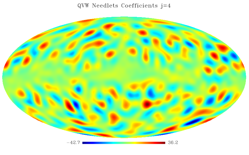
In Fig. 1 we show the needlet coefficients of WMAP 5-year temperature map for and . The anomalous bright spots found by Pietrobon et al. (2008) are clearly visible.
We next briefly review the properties of the needlet bispectrum and how it relates to the usual bispectrum. An extensive discussion is provided in Lan & Marinucci (2008); Rudjord et al. (2009a). See also Pietrobon et al. (2009). The needlet estimator is defined as follows:
| (6) |
where means the pixels outside the mask and is estimated bispectrum, averaged over s. can be seen as a binned bispectrum, a smooth and combined component of the angular bispectrum. We divide these bispectrum measurements into four classes based on their geometries: equilateral (equi) configurations have three equal values, isosceles configurations (iso) have two legs equal (e.g. ), while scalene configurations (scal) have three different legs. Finally we also consider open configurations, for which , and do not form a triangle (e.g. ); naively these might be expected to be zero, but since each includes a range of values, these could include signals arising from , and which just satisfy the triangle relations. Thus open configurations correspond to the most co-linear geometries. This must be kept in mind for all the configurations; e.g., while the equilateral -configurations will be dominated by triangles roughly equilateral in , they will also have contributions from other geometries. Separating the needlet bispectrum by the above described configurations may provide insight into the physical origin of possible anomalies. For instance Ackerman et al. (2007) and Erickcek et al. (2008) suggest early Universe models which could produce a statistically anisotropic CMB sky.
3 Statistical Analysis and Results for WMAP 5-year Data
Next we describe the simulations used in our needlet bispectrum analysis. We start by producing simulated Gaussian CMB maps taking into account the beam and the noise properties of each WMAP-5111http://lambda.gsfc.nasa.gov/product/map/dr3/m_products.cfm channel Q, V and W. From these single-channel maps we construct an optimal map (see Jarosik et al. (2007)), where represents a direction on the sky and where is the number of observations of a given pixel and the nominal sensitivity of the channel (Hinshaw et al., 2009). We apply the “-”Kq75 combined mask described by Pietrobon et al. (2008) and degrade the resulting map to the resolution of . We extract the needlet coefficients from the simulated maps for a given and compute the needlet bispectrum of the reconstructed coefficient maps according to Eq. 2. Finally, we calculate from the real data of the foreground-reduced WMAP 5-year Q, V and W channels data, using the same procedure applied to the simulated maps. To test the Gaussianity of WMAP 5-year data, we compare the distribution of the of the simulated dataset to the value obtained from data, where is the array consisting of the needlet bispectrum values calculated via Eq. 2. We consider the needlet bispectrum values (indicated by “all” in the tables)’ and, to identify where the anomalies are concentrated, we split the analysis in different branches according to the geometry of the triangles. For the chosen , we have 115 which satisfy the requirements: 9 equilateral, 56 isosceles, 50 scalene. We define the remaining 50 configurations as open: we would expect them to be vanishing except for those which combine multipoles which fulfill the Wigner selection rules. The correspondence between each needlet scale and its multipole range is shown in Table 1.
| Large Scales | |||||
|---|---|---|---|---|---|
| 1 | 2 | 3 | 4 | 5 | |
| Small Scales | |||||
| 6 | 7 | 8 | 9 | ||
| - | |||||
On the full CMB sky, the of the data is compatible with the distribution we obtain from 20,000 Gaussian simulations. When we calculate the on the northern and southern hemispheres separately, we find a significant deviation from Gaussianity in the southern hemisphere while the northern hemisphere appears Gaussian, having a bispectrum generally somewhat smaller than expected (see Table 2). The results are shown in the histogram plots in Fig. 2.
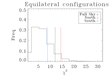
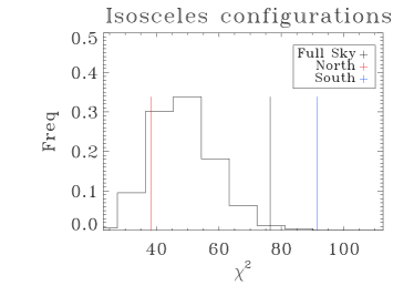
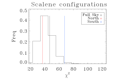
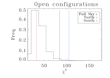
Furthermore, considering the triangle configurations as classified above, we found that this behaviour is concentrated in all triangle configurations separately except for the equilateral ones. The isosceles triangles are perhaps the most interesting ones since they probe the correlation between the large and the small angular scales (the so-called ‘squeezed’ configurations), which should reflect a non-local type of non-Gaussianity. A comparable degree of asymmetry is shown by scalene and open configurations, which confirm the global lack of power in the north hemisphere: the points in the northern hemisphere show a lower scatter. A similar asymmetric behaviour was found by Hansen et al. (2004); Land & Magueijo (2005); Eriksen et al. (2004) and recently confirmed by Hoftuft et al. (2009); Hansen et al. (2009); Groeneboom & Eriksen (2009). In our analysis we already mask the big anomalous features present in the southern hemisphere, responsible for about 50% of the power asymmetry in the angular power spectrum (Pietrobon et al., 2008). The results are summed in Table 2.
| conf. | FULL SKY | NORTH | SOUTH |
|---|---|---|---|
| all (115) | |||
| equi (9) | |||
| iso (56) | |||
| scal (50) | |||
| open (50) |
Note that equilateral configurations are directly related to the skewness of the needlet coefficient distributions: the fact that on the whole sky we do not find a strong deviation from Gaussianity is in agreement with the previous literature, where only the kurtosis of the distributions showed an anomalous behavior (see Vielva et al. (2004)).
Large-Small Scale Analysis.
Going more deeply, we focused on small and large angular scales separately. In particular, with the choice , we define the subset of needlets to as large scale, corresponding roughly to scales larger than 1 degree; while the subset to corresponds to the sub-degree scales (see Table 1). We then perform the same analysis we carried out on the whole needlet set. The results are shown in Table 3. The isosceles configurations still show a large difference between the two hemispheres but the significance is lower than the whole set analysis. The open configuration result is still anomalous.
| conf. | Large Scales () | ||
|---|---|---|---|
| FULL SKY | NORTH | SOUTH | |
| all (28) | |||
| equi (5) | |||
| iso (16) | |||
| scal (7) | |||
| open (7) | |||
| conf. | Small Scales () | ||
| FULL SKY | NORTH | SOUTH | |
| all (20) | |||
| equi (4) | |||
| iso (12) | |||
| scal (4) | |||
No open configurations exist for the small scale subset ; however for the large scales these co-linear configurations are most significantly non-zero for the biggest contribution of the power. For the sub-degree set we did not find an high degree of anomaly, as summarised in Tab. 3, though the isosceles configurations are still significantly different between the two hemispheres. Dividing the analysis between the two sets at large and small scales, we miss the important contribution given by the correlation between the two, which is indeed crucial for the squeezed triangles. We then consider two more sets: one formed by triangles with one side and two sides belonging to the small scale set (,). We label this set as LSS and are predominantly squeezed. The second set, labelled as LLS, is formed by triangles which have , and and are predominantly co-linear. We report the results in Tab. 4.
| conf. | Correlation (L-S-S) | ||
|---|---|---|---|
| FULL SKY | NORTH | SOUTH | |
| iso (20) | |||
| scal (26) | |||
| open (4) | |||
| conf. | Correlation (L-L-S) | ||
| FULL SKY | NORTH | SOUTH | |
| iso (8) | |||
| scal (13) | |||
| open (39) | |||
The isosceles triangles belonging to the LSS set are very anomalous in the south hemisphere. The LLS set in characterised by an anomaly in the open configurations. Interestingly the lack of signal in the northern hemisphere is evident in the LLS, while the LSS distribution appears more typical.
Further analysis.
Since the first anomalies were found, several methods have been applied to search for a specific direction in the sky which maximises the asymmetry. Indeed, many works identify a direction very close to the ecliptic poles (Hansen et al., 2004; Land & Magueijo, 2005; Räth et al., 2009; Hansen et al., 2009). In particular a dipole modulation has been proposed as a possible explanation for such pattern in (Hoftuft et al., 2009). In order to see whether a similar modulation underlies the asymmetry we detect, we rotated the reference frame, spanning uniformly the sky, and recomputed our statistics for the WMAP data with the new north-south definition. Since the set of simulations we used assume isotropy and homogeneity, the rotation of the reference frame does not affect their statistics and the covariance matrix we applied in our previous analysis.
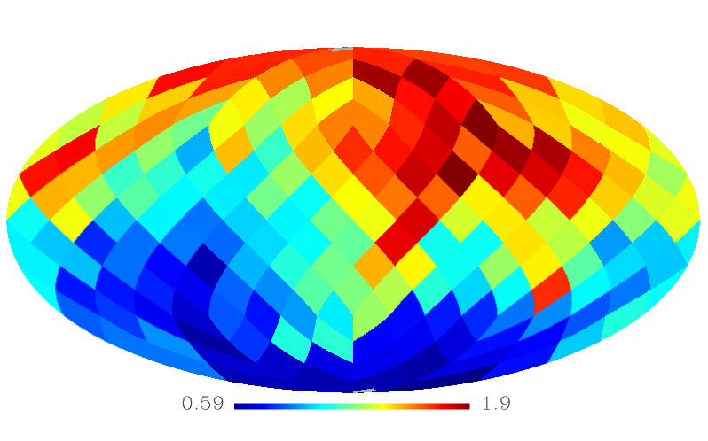
The result is shown in Fig. 3, where we plotted the reduced for the southern hemisphere in the particular case of the isosceles configurations, as a function of the north pole direction. We chose the isosceles triangles since they show the highest degree of asymmetry. A pattern is clearly visible, but the direction which maximises the anomaly seems to be orthogonal to the one reported by other authors with different estimators. This may suggest that either the 3-point correlation function couples differently to the dipole modulation, or the nature of the asymmetry we measured is different. Whether this direction depends upon the shape and the angular scale we consider, its significance and the link with the direction found in literature are interesting questions, which require a dedicated study and they will be addressed in a following paper.
Finally, we checked whether the sky asymmetries we detected affect the measure of the primordial non-Gaussianity parameter. A complete review on the nature of this parameter may be found in Bartolo et al. (2004) and Fergusson & Shellard (2008); recent constraints from CMB experiments can be found in Smith et al. (2009); Curto et al. (2008); Komatsu et al. (2009); de Troia et al. (2007) while Slosar et al. (2008) constrained through the galaxy distribution. Limits on using wavelets are discussed in Curto et al. (2009); Cabella et al. (2004); Mukherjee & Wang (2004). We estimate performing the same analysis described in Pietrobon et al. (2009), applying the estimator
| (7) |
to the WMAP 5-year dataset. Here X is a vector composed by the values of needlets bispectrum for a given triangular configuration according to Eq.2. The covariance matrix is calculated from 20.000 Gaussian simulations, since its dependency on is negligible (e.g. see Spergel & Goldberg (1999)). The theoretical non-Gaussian template was calculated via Monte Carlo simulations over the 100 primordial non-Gaussian maps (Liguori et al., 2007). Since we know the CMB sky is asymmetric, showing more non-Gaussianity in the southern hemisphere, we carried out a split north-south analysis to see if the asymmetry extends to differences in the estimate. Recently, Curto et al. (2009) and Rudjord et al. (2009b) targeted the same issue, finding no evidence of varying on the sky.We do not find a significant deviation between the values measured in the two hemispheres, while the error bars become significantly larger due to the reduced number of pixels used to calculate the needlet bispectrum.
4 Conclusions
In this paper we used the needlets bispectrum to investigate the presence of anomalies in the WMAP 5-year data. For the first time we exploited the bispectrum formalism analysing the triangle configurations according to their shape. By splitting the analysis of the needlets bispectrum for the northern and southern hemispheres we found that the southern sky is barely compatible with the Gaussian hypothesis while the northern hemisphere is characterised by a lack of global bispectrum signal. This is complementary to what found by applying different statistics: power spectra (Hansen et al., 2009), bispectrum (Land & Magueijo, 2005) and n-point correlation functions (Eriksen et al., 2005). We distinguished equilateral, isosceles, scalene and open configurations and compared the power present in the data to random Gaussian simulations. The most anomalous signals in the southern Galactic hemisphere arise in the squeezed configurations (isosceles, large-small-small) and in the very co-linear configurations (open, large-large-small). This kind of information should be useful as a means to find out the physical origin of the anomalies. While the large squeezed signal hints at a local type of non-Gaussianity, this is not bourne out when an optimal estimator tuned specifically to this type of non-Gaussianity is used. We investigated the effect of hemispherical asymmetry on the measurement of finding no significant discrepancy between north and south. As consistency check, we performed the same tests (anomalies and estimates) with a different needlets parameter () and for the channels Q,V and W separately and found consistent results.
Acknowledgements
We thank Frode K. Hansen, Michele Liguori and Sabino Matarrese for providing us with the primordial non-Gaussian map dataset. We are grateful to Domenico Marinucci and Marcella Veneziani for useful discussions. The ASI contract LFI activity of Phase2 is acknowledged.
References
- Ackerman et al. (2007) Ackerman L., Carroll S. M., Wise M. B., 2007, Phys. Rev., D75, 083502
- Baldi et al. (2006) Baldi P., et al., 2006, Annals of Statistics 2009, Vol. 37, No. 3, 1150-1171
- Bartolo et al. (2004) Bartolo N., et al., 2004, Phys. Rept., 402, 103
- Bennett et al. (2003) Bennett C. L., et al., 2003, ApJ, 148, 1
- Bernui et al. (2007) Bernui A., et al., 2007, Int. J. Mod. Phys., D16, 411
- Bernui & Reboucas (2009) Bernui A., Reboucas M. J., 2009, Phys. Rev., D79, 063528
- Cabella et al. (2004) Cabella P., et al., 2004, Phys. Rev. D., 69, 063007
- Copi et al. (2007) Copi C., et al., 2007, Phys. Rev. D., 75, 023507
- Cruz et al. (2005) Cruz M., et al., 2005, MNRAS, 356, 29
- Curto et al. (2008) Curto A., et al., 2008, A&A, 486, 383
- Curto et al. (2009) Curto A., Martinez-Gonzalez E., Barreiro R. B., 2009, arXiv: 0902.1523
- de Oliveira-Costa et al. (2004) de Oliveira-Costa A., et al., 2004, Phys. Rev. D., 69, 063516
- de Troia et al. (2007) de Troia G., et al. 2007, ApJ, 670, L73
- Erickcek et al. (2008) Erickcek A. L., Kamionkowski M., Carroll S. M., 2008, Phys. Rev. D., 78, 123520
- Eriksen et al. (2004) Eriksen H. K., et al., 2004, Astrophys. J., 605, 14
- Eriksen et al. (2004) Eriksen H. K., et al., 2004, ApJ, 609, 1198
- Eriksen et al. (2005) Eriksen H. K., et al., 2005, ApJ, 622, 58
- Faÿ et al. (2008) Faÿ G., et al., 2008, Phys. Rev. D., 78, 083013
- Fergusson & Shellard (2008) Fergusson J. R., Shellard E. P. S., 2008, arXiv: 0812.3413
- Geller & Marinucci (2008) Geller D., Marinucci D., 2008, arXiv:math/0811.2935
- Groeneboom & Eriksen (2009) Groeneboom N. E., Eriksen H. K., 2009, ApJ, 690, 1807
- Guilloux et al. (2007) Guilloux F., Fay G., Cardoso J.-F., 2007, arXiv: 0706.2598
- Hansen et al. (2004) Hansen F. K., Banday A. J., Górski K. M., 2004, MNRAS, 354, 641
- Hansen et al. (2004) Hansen F. K., et al., 2004, ApJ, 607, L67
- Hansen et al. (2009) Hansen F. K., et al., 2009, ApJ, 704, 1448
- Hinshaw et al. (2009) Hinshaw G., et al., 2009, ApJ, 180, 225
- Hoftuft et al. (2009) Hoftuft J., et al., 2009, arXiv: 0903.1229
- Jarosik et al. (2007) Jarosik N., et al. 2007, ApJ, 170, 263
- Komatsu et al. (2009) Komatsu E., et al., 2009, ApJ, 180, 330
- Lan & Marinucci (2008) Lan X., Marinucci D., 2008, Elec. Jour. of Stats. 2008, Vol. 2, 332-367, 802
- Land & Magueijo (2005) Land K., Magueijo J., 2005, MNRAS, 357, 994
- Land & Magueijo (2007) Land K., Magueijo J., 2007, MNRAS, 378, 153
- Lew (2008) Lew B., 2008, JCAP, 0809, 023
- Liguori et al. (2007) Liguori M., et al., 2007, Phys. Rev. D., 76, 105016
- Marinucci et al. (2008) Marinucci D., et al., 2008, MNRAS, 383, 539
- McEwen et al. (2008) McEwen J. D., et al., 2008, MNRAS, 388, 659
- Moudden et al. (2005) Moudden Y., et al., 2005, EURASIP J. Appl. Signal Process., 15, 2437
- Mukherjee & Wang (2004) Mukherjee P., Wang Y., 2004, ApJ, 613, 51
- Narcowich et al. (2006) Narcowich F. J., Petrushev P., Ward J. D., 2006, SIAM J. Math. Anal., 38, 574
- Nolta et al. (2009) Nolta M. R., et al., 2009, ApJ, 180, 296
- Park (2004) Park C.-G., 2004, MNRAS, 349, 313
- Pietrobon et al. (2006) Pietrobon D., Balbi A., Marinucci D., 2006, Phys. Rev. D., 74, 043524
- Pietrobon et al. (2008) Pietrobon D., et al., 2008, Phys. Rev. D., 78, 103504
- Pietrobon et al. (2009) Pietrobon D., et al., 2009, MNRAS, 396, 1682
- Räth et al. (2009) Räth C., et al., 2009, Physical Review Letters, 102, 131301
- Rossmanith et al. (2009) Rossmanith G., et al., 2009, MNRAS, pp 1330–+
- Rudjord et al. (2009a) Rudjord O., et al., 2009a, arXiv: 0901.3154
- Rudjord et al. (2009b) Rudjord Ø., et al., 2009b, arXiv: 0906.3232 (CO)
- Slosar et al. (2008) Slosar A., et al., 2008, JCAP, 8, 31
- Smith et al. (2009) Smith K. M., Senatore L., Zaldarriaga M., 2009, arXiv: 0901.2572
- Spergel et al. (2007) Spergel D. N., et al., 2007, ApJ, 170, 377
- Spergel & Goldberg (1999) Spergel D. N., Goldberg D. M., 1999, Phys. Rev. D., 59, 103001
- Vielva et al. (2004) Vielva P., et al., 2004, ApJ, 609, 22