Fisher Matrix Decomposition for Dark Energy Prediction

Abstract

Within the context of constraining an expansion of the dark energy equation of state $w(z)$ we show that the eigendecomposition of Fisher matrices is sensitive to both the maximum order of the expansion and the basis set choice. We investigate the Fisher matrix formalism in the case that a particular function is expanded in some basis set. As an example we show results for an all sky weak lensing tomographic experiment. We show that the set of eigenfunctions is not unique and that the best constrained functions are only reproduced accurately at very higher order $N\mathrel{\raise 1.16pt\hbox{$>$}\kern-7.0pt\lower 3.06pt\hbox{{$\scriptstyle\sim$}}}100$, a tophat basis set requires an even higher order. We show that the common approach used for finding the marginalised eigenfunction errors is sensitive to the choice of non-$w(z)$ parameters and priors. The eigendecomposition of Fisher matrices is a potentially useful tool that can be used to determine the predicted accuracy with which an experiment could constrain $w(z)$. It also allows for the reconstruction of the redshift sensitivity of the experiment to changes in $w(z)$. However the technique is sensitive to both the order and the basis set choice. Publicly available code is available as part of iCosmo at http://www.icosmo.org.

1 Introduction

The Fisher matrix methodology (Tegmark, Taylor & Heavens, 1997; Jungman et al., 1996; Fisher, 1935) is a statistical tool that has been used with some success in predicting the ability of future experiments to constrain particular parameters of interest. In cosmology Fisher matrices have gained some importance in predicting the potential outcome of experiments, in particular dark energy surveys, on which a large amount of resources may be spent. It is therefore of paramount importance that the way in which Fisher matrices are used should be understood and that any results that depend on this methodology should be robust and reliable.

In this article we will outline how the techniques of decomposing a general matrix have a special interpretation when used within the Fisher matrix framework. This will be done within the context of attempting to predict constraints for an extended parameter set. We will use the specific example of attempting to constrain dark energy equation of state $w(z)$ parameters (Albrecht & Bernstein, 2007; Tang et al., 2008; Simpson & Bridle, 2006; Crittenden & Pogosian, 2005; de Putter & Linder, 2008; Dick et al., 2006; Huterer & Cooray, 2005; Huterer & Starkman, 2003; Hu, 2002; Knox et al., 2005; Ishak et al. 2006; Zhan et al., 2009a; Zhan et al., 2009b; Cunha et al., 2009; Joudaki et al., 2009; Sarkar et al., 2008), most recently Albrecht et al. (2009) defined a new dark energy Figure of Merit using a binned $36$ parameter model.

We will show that the eigenfunctions obtained by diagonalising a Fisher matrix are dependent of the basis set used in the construction of the Fisher matrix, and that the eigenfunctions only tend to agreement in the limit of a very large order of expansion. We will also show that the usual method of marginalising over extra parameters – constructing the Schur complement (Zhang, 2005) of the total Fisher matrix – is dependent on the choice of non-$w(z)$ parameterisation and priors when also performing an eigendecomposition.

In Section 2 we will introduce the methodology, in Section 3 we will apply the approach to weak lensing tomographic survey prediction, we present conclusions in Section 4.

2 Methodology

For a set of parameters $\mn@boldsymbol{\theta}$ the Fisher matrix allows for the prediction of parameter errors given a specific experimental design and method for extracting parameters. In the case of Gaussian-distributed data where we assume that the error on the signal is not a function of parameter values $\sigma_{C}\not=\sigma_{C}(\mn@boldsymbol{\theta})$ we can take the covariance of the estimated values of the parameters;

$${\rm cov}[\mn@boldsymbol{\theta}_{i},\mn@boldsymbol{\theta}_{j}]=\langle(\mn@boldsymbol{\theta}_{i}-\langle\mn@boldsymbol{\theta}_{i}\rangle)(\mn@boldsymbol{\theta}_{j}-\langle\mn@boldsymbol{\theta}_{j}\rangle)\rangle=F^{-1}_{ij},$$ (1)

where the Fisher matrix is defined by (Tegmark, Taylor & Heavens, 1997; Jungman et al., 1996; Fisher, 1935)

$$F_{ij}=\sum_{x}\left[\sigma^{-2}_{C}\frac{\partial S}{\partial\mn@boldsymbol{\theta}_{i}}\frac{\partial S}{\partial\mn@boldsymbol{\theta}_{j}}\right],$$ (2)

where $S$ is the signal. The predicted marginal errors on the parameters are given by $\Delta\theta_{i}=\sqrt{(F^{-1})_{ii}}$, this is the minimum marginal error that one can expect for the method and experimental design considered (due to the lower bound in the Cramer-Rao inequality).

If we extend the parameter set to $\mbox{\boldmath$\phi$}=(\mn@boldsymbol{\theta}$, $\mbox{\boldmath$\psi$})$ then the Fisher matrix is extended to include these extra parameters

$$F^{\mbox{\boldmath$\phi$}\mbox{\boldmath$\phi$}}=\left(\begin{array}[]{cc}F^{\mn@boldsymbol{\theta}\mn@boldsymbol{\theta}}&F^{\mn@boldsymbol{\theta}\mbox{\boldmath$\psi$}}\\ F^{\mbox{\boldmath$\psi$}\mn@boldsymbol{\theta}}&F^{\mbox{\boldmath$\psi$}\mbox{\boldmath$\psi$}}\\ \end{array}\right)$$ (3)

and the predicted marginal errors on the parameters $\Delta\theta_{i}=\sqrt{(F^{-1})^{\mbox{\boldmath$\phi$}\mbox{\boldmath$\phi$}}_{ii}}$ are increased due to degeneracies between the original parameters and the new parameters.

For dark energy cosmology prediction the parameter set is commonly divided into those that contain information on the dark energy equation of state $w(z)$ and those that do not. The usual approach taken (Albrecht et al., 2009; Albrecht & Bernstein, 2007; Tang et al., 2008; Simpson & Bridle, 2006; Crittenden & Pogosian, 2005; de Putter & Linder, 2008; Dick et al., 2006; Huterer & Cooray, 2005; Huterer & Starkman, 2003; Hu, 2002; Knox et al., 2005; Ishak et al. 2006; Zhan et al., 2009a; Zhan et al., 2009b; Cunha et al., 2009; Joudaki et al., 2009; Sarkar et al., 2008) is to “bin” $w(z)$ in redshift and to assign an amplitude to the value of $w(z)$ in each bin. However $w(z)$ is not a directly observable quantity but can only be inferred through other integral relations, most simply the comoving distance or Hubble parameter

$$D(z)=\frac{c}{H_{0}}\int_{0}^{z}{\rm d}z\frac{1}{(\Omega_{m}(1+z)^{3}+\Omega_{\rm de}{\rm e}^{3\int_{0}^{z}{\rm d}z^{\prime}[1+w(z^{\prime})]/(1+z^{\prime})})^{\frac{1}{2}}}$$ (4)

$$H(z)=H_{0}(\Omega_{m}(1+z)^{3}+\Omega_{\rm de}{\rm e}^{3\int_{0}^{z}{\rm d}z^{\prime}[1+w(z^{\prime})]/(1+z^{\prime})})^{\frac{1}{2}}.$$ (5)

So any binned expansion of $w(z)$ to include extra parameters cannot be justified by arguing that the data itself is binned in redshift.

The choice of how to expand the function $w(z)$ is thus a purely theoretical one. In general we will consider $w(z)$ expanded in some complete basis set

$$1+w(z)=\sum_{i=1}^{\infty}a_{n}\phi_{n}(z),$$ (6)

where $a_{n}$ are the basis coefficients and $\phi_{n}$ are the basis functions. Since we do not know what dark energy equation state is apt for the physical Universe any chosen basis set is as valid as any other. Binning is a special case where the basis functions are tophat functions in redshift

$$\phi_{n}^{\rm binning}(z)={\mathcal{H}}(z-\frac{\Delta z}{2})-{\mathcal{H}}(z+\frac{\Delta z}{2}),$$ (7)

where $\Delta z$ is the bin width and ${\mathcal{H}}$ is the Heaviside (step) function.

Figure 1: An example of the residual that can occur when reconstructing a given basis sets functions with another basis set. On the y axes are the order of the basis function to be reconstructed, on the x axes are the maximum order of the series that is attempting to reconstruct the functions. The gray scale shows the maximum residual (black low residual, whit large residual), each function is investigated over the range $x\in[-1,1]$. The left plot shows the order of Chebyshev polynomials needed to reconstruct Legendre polynomials. The middle plot shows the order of Legendre polynomials needed to reconstruct Chebyshev polynomials (the inverse operation to the left plot). The right hand plot shows the order of the tophat basis set needed to reconstruct Chebyshev polynomials. The red (gray vertical) lines are at $N=36$ (Albrect et al., 2009) to guide the reader.

Note that interpolations between delta function values at discrete redshifts, linearly or with some spline function, are different basis sets to binning. We clarify three broad meanings of binning that occur in the literature

• Tophat basis set : functions are not continuous, all derivatives are ill-defined.

• Linear interpolation : functions are continuous, $1^{{\rm st}}$ derivatives are discontinuous, $2^{{\rm nd}}$ and higher order derivatives are ill-defined.

• Spline (e.g. quadratic spline) : functions are continuous, $1^{{\rm st}}$ derivatives are continuous, $2^{{\rm nd}}$ derivatives are discontinuous, $3^{{\rm rd}}$ derivatives and higher are ill-defined.

Of these three basis functions, only tophat form an orthogonal basis set; though all form a complete basis set. We include interpolation in Section 3 for completeness, and because it is commonly used in the literature.

The most general condition that we could apply to the expected $w(z)$ is that it is continuous (features could be very sharp in redshift but not physically discontinuous – the sound speed of dark energy is generally expected to be $\leq c$). We note that binning is not discrete differentiable since at the bin boundary the gradient is infinite.

We will now investigate how the Fisher matrix should be treated when such an expanded basis set is used.

2.1 Basis set decomposition

The general framework with which we are now presented consists of a Fisher matrix

$$F=\left(\begin{array}[]{cc}F^{\mn@boldsymbol{\theta}\mn@boldsymbol{\theta}}&F^{\mn@boldsymbol{\theta}\mbox{\boldmath$w$}(\phi)}\\ F^{\mbox{\boldmath$w$}(\phi)\mn@boldsymbol{\theta}}&F^{\mbox{\boldmath$w$}(\phi)\mbox{\boldmath$w$}(\phi)}\\ \end{array}\right),$$ (8)

where $\mn@boldsymbol{\theta}$ are the cosmological parameters not associated with $w(z)$. $\mbox{\boldmath$w$}(\phi)$ are the set of parameters that describe $w(z)$ where we have expanded $w(z)$ using a general complete orthogonal basis set with basis functions $\phi$. The sub-Fisher matrix for $w(z)$ is calculated by

$$F^{\mbox{\boldmath$w$}(\phi)\mbox{\boldmath$w$}(\phi)}=\sum_{x}\frac{1}{\sigma(x)^{2}}\frac{\partial S}{\partial a_{i}}\frac{\partial S}{\partial a_{j}},$$ (9)

where $\sigma(x)$ is the expected marginal error on the signal $S$ and the errors on the coefficients of the expansion (equation 6) $\sqrt{(F^{\mbox{\boldmath$w$}(\phi)\mbox{\boldmath$w$}(\phi)})^{-1}_{ii}}=\Delta a_{i}$ (not marginalising over non-$w(z)$ parameters $\mn@boldsymbol{\theta}$).

A basis set is orthogonal if it satisfies the orthogonality relationship

$$\int_{R}\phi_{m}(z)\phi_{n}(z)M(z){\rm d}z=c_{m}\delta^{K}_{mn},$$ (10)

over a range $R$, where $M(z)$ is a weighting function, $c_{m}$ are constants and $\delta^{K}_{mn}$ is the Kronecker delta. The coefficients needed to construct an arbitrary function $f(z)$ using the basis set $\phi$ are given by

$$a_{n}=\frac{1}{c_{n}}\int_{R}f(z)\phi_{n}(z)M(z){\rm d}z.$$ (11)

In general we can construct the Fisher matrix (equation 8) using an orthogonal basis set for $w(z)$ (orthogonal with respect to a weight function $M(z)$) but the sub-matrix $F^{\mbox{\boldmath$w$}(\phi)\mbox{\boldmath$w$}(\phi)}$ will not be diagonal since $w(z)$ can, at a minimum, only be observed through integral relations.

A common approach is to look for the eigenfunctions of $w(z)$. The motivation for this is that the eigenfunctions are thought to form an orthogonal basis set. These functions are found by rotating the Fisher matrix such that it is diagonalised using the transformation

$$\Lambda^{\phi} = Q^{T}FQ$$

$$F = Q\Lambda^{\phi}Q^{T},$$ (12)

where Q is an orthogonal matrix, $Q^{T}Q=I$.

By performing this transformation the non-$w(z)$ errors can also affected. There a three possibilities: either $F$ is the full $w$ and non-$w$ Fisher matrix in which case the non-$w$ parameters are clearly affected, or $F$ is the $w$-only Fisher matrix, or $F$ can be the marginalised $w$-only Fisher matrix. We discuss these later two options in Section 2.3.

The new Fisher matrix $\Lambda^{\phi}$ is a diagonal matrix. The $Q$ matrices are called the eigenmatrices (or vectors) which are a special kind of Jacobian matrix in which the original matrix is rotated such that is diagonalised (see Appendix A). In performing this operation we have constructed a new set of basis functions, $e$, that are linear combinations of the original basis set, $\phi$. $w(z)$ can now be reconstructed using two equivalent forms

$$1+w(z)=\sum_{n=1}^{N}a_{n}\phi_{n}(z)=\sum_{n=1}^{N}b_{n}e_{n}(z)$$ (13)

where $N$ is the order of the sub-Fisher matrix $F^{\mbox{\boldmath$w$}(\phi)\mbox{\boldmath$w$}(\phi)}$ – we have introduced this maximum order since Fisher matrices have, by definition, a finite order. The new functions, $e$, can be constructed using the eigenmatrix

$$e_{i}(z)=\sum_{j=1}^{N}Q_{ij}\phi_{j}(z)$$ (14)

where (Appendix A)

$$Q_{ij}=\frac{\partial b_{j}}{\partial a_{i}}.$$ (15)

The new Fisher matrix has diagonal elements that are related to the errors on the new functions’ coefficients

$$\Lambda^{\phi}_{ij}=\sum_{x}\frac{1}{\sigma(x)^{2}}\frac{\partial S}{\partial b_{i}}\frac{\partial S}{\partial b_{j}}=\delta^{K}_{ij}\frac{1}{(\Delta b_{i})^{2}}.$$ (16)

In performing such a rotation we have effectively created a new basis set that is orthogonal with respect to a new weight function (equation 10) that takes into account the covariance in the Fisher matrix.

We note that an operation of the form $F=Q\Lambda Q^{T}$ (or the inverse $Q^{T}FQ=\Lambda$) leads to a unique $Q$ if $\Lambda$ and $F$ are fixed. However in general a further operator $P$ can be applied to the new diagonal matrix $P\Lambda=P(Q^{T}FQ)$ to map a matrix $F$ to any diagonal of the same dimension, where $P$ is also a diagonal. $P$ acts like a ‘stretching’ (or compression), not a rotating, operator. $P$ does not correspond to a change in parameters but a change in the errors on an eigenbasis parameter set. We do not consider this in the remainder of the article.

We also note that in general there exists operators that can rotate from a large matrix to a smaller one. For example an $n\times n$ diagonal matrix $\Lambda^{\rm large}$ can be mapped to a smaller $m\times m$ diagonal matrix $\Lambda^{\rm small}$ where $m<n$ via the operator $\Lambda^{\rm small}_{kk}=A_{ki}\Lambda^{\rm large}_{ii}A^{T}_{ik}$ where $A_{ki}$ is an $n\times m$ matrix. So if the size of the matrices are not specified then the operation $F=A(Q\Lambda Q^{T})A^{T}=R\Lambda R^{T}$ (where $R=AQ$) can map a matrix to a diagonal of smaller dimension. This is equivalent to mapping the basis set expansion from a particular order to one of a smaller maximum order. Note that this is in general a one-way operation since information is lost in the minimisation. In the remainder of this article we will only consider mapping between matrices of the same dimension.

2.2 The non-uniqueness of the eigenfunctions

It is often assumed that an eigenfunction decomposition yields a set of functions that are unique (if they are not degenerate; Albrecht et al., 2009; Crittenden & Pogosian, 2005; Huterer & Starkman, 2003). This statement comes from matrix theory; the diagonalisation of a particular matrix can only be done one way. However this does not mean that the eigenfunctions of $w(z)$ from a finite Fisher matrix are unique, since we can start with different basis sets and this choice is arbitrary. This break-down is due to the finite number of coefficients - so is really a convergence statement.

The general minimum assumption case we are dealing with is one in which we consider two Fisher matrices calculated by expanding $w(z)$ in two different basis sets $\phi$ and $\psi$.

We can only transform one Fisher matrix $F^{\phi}\rightarrow F^{\psi}$ to another by changing the basis sets if all the basis set $\phi$ functions $1\rightarrow N$ can be described using only the functions $1\rightarrow N$ from the set $\psi$, and vice versa. For example to rotate from basis $\phi$ to $\psi$ then

$$\psi_{i}(x)\equiv\sum_{j=1}^{N}J_{ij}\phi_{j}(x)\ \ \ \ \ \forall\ \ 1\leq i\leq N$$ (17)

needs to be true. However for any conceivable complete basis set for finite $N$ this sum will always have some residual. This residual $R_{i}(x)$ can be quantified by

$$\psi_{i}(x)=\sum_{j=1}^{N}J_{ij}\phi_{j}(x)+R_{i}(x)$$

$$R_{i}(x)=\sum_{n=N+1}^{\infty}\left(\frac{1}{c^{\phi}}\int_{R}{\rm d}x^{\prime}\psi_{i}(x^{\prime})\phi_{n}(x^{\prime})M^{\phi}(x^{\prime})\right)\phi_{n}(x).$$ (18)

The notation we use throughout is that $Q$ are explicitly eigenmatrices, $J$ are explicitly general Jacobian transformations, $R$ are residuals and $F$ are Fisher matrices. Note however that an eigenmatrix $Q$ is a special kind of Jacobian $J$ where the result of the transformation is a diagonal.

In Appendix B we show that if the residual is non-zero then the eigenvalues are not equal.

If the residual between any two basis sets is small, in the limit of large $N$, then the eigenfunctions will agree to some accuracy, and one would expect the best constrained eigenfunctions from any basis set to converge. However for a finite $N$ the eigenfunctions will only all agree if the $N^{\rm th}$ basis function in one set can be reproduced using only the functions $1\rightarrow N$ in other basis set.

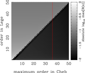
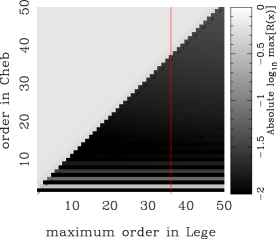
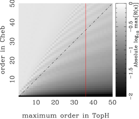
Figure 1 shows the residuals (equation 2.2) between a variety of basis sets as a function of order (in equation 2.2 we replaced $\infty$ with $10^{7}$ for which we find numerical convergence of the results in this Figure since $50\ll 10^{7}$). This plot shows that in order to have a residual of $<0.01$ when reconstructing Legendre polynomials with Chebyshev the order of the Chebyshev needs to be at least as high as the order of the basis function that is being reconstructed. However in the opposite case the low order Chebyshev polynomials are difficult to reproduce with Legendre, and the Chebyshev polynomials are difficult to reproduce with the tophat basis set (binning). In fact Cheyshev functions are more difficult to reproduce (especially at low order) because they are bounded in the $y$ direction as well as the $x$ direction.

If one chooses a maximum order of $N=36$ (Albrecht et al., 2009) for example then there would be $>0.01$ residual in reconstructing Chebyshev, Legendre and tophat basis sets from each other. As a result the reconstructed eigen functions would not agree. We will investigate this further in Section 3.

To summarise this section

• The eigenfunctions created using two different basis sets and a finite order will only agree if the residual between the reconstruction of the basis functions is zero.

• For a finite order there will always exist some eigenfunctions from a given basis set that cannot be reproduced using another. So for finite order the set of eigenfunctions is non-unique.

• For a large finite order we expect the best constrained eigen functions to tend to agreement, and for this agreement to improve as the order is increased.

2.3 Marginalisation

Another difficulty in constructing robust eigenfunctions is deciding what to do with the non-$w(z)$ parameters. A common approach is to marginalise over these other parameters and then perform the eigenfunction decomposition. This in effect mixes all of these parameters with the equation of state expansion.

Referring to equation (8) if we want to know the errors on expanded $w(z)$ parameters then we can marginalise over the other parameters $\mn@boldsymbol{\theta}$ by constructing the Schur complement (Zhang, 2005) of the $F^{\mbox{\boldmath$w$}(\phi)\mbox{\boldmath$w$}(\phi)}$ sub-matrix

$$F^{\mbox{\boldmath$w$}(\phi)\mbox{\boldmath$w$}(\phi)}_{1S}=F^{\mbox{\boldmath$w$}(\phi)\mbox{\boldmath$w$}(\phi)}-F^{\mbox{\boldmath$w$}(\phi)\mn@boldsymbol{\theta}}(F^{\mn@boldsymbol{\theta}\mn@boldsymbol{\theta}})^{-1}F^{\mn@boldsymbol{\theta}\mbox{\boldmath$w$}(\phi)}.$$ (19)

The new Fisher matrix $F^{\mbox{\boldmath$w$}(\phi)\mbox{\boldmath$w$}(\phi)}_{1S}$ will then give errors on the $w(z)$ parameters already marginalised over the extra parameters.

We can now diagonalise $F^{\mbox{\boldmath$w$}(\phi)\mbox{\boldmath$w$}(\phi)}_{1S}$ like

$${\rm diag}(F_{1S}^{\mbox{\boldmath$w$}(\phi)\mbox{\boldmath$w$}(\phi)}) = (Q^{\rm mixed})^{T}F^{\mbox{\boldmath$w$}(\phi)\mbox{\boldmath$w$}(\phi)}Q^{\rm mixed}$$ (20)

$$- (Q^{\rm mixed})^{T}F^{\mn@boldsymbol{\theta}\mbox{\boldmath$w$}(\phi)}(F^{\mn@boldsymbol{\theta}\mn@boldsymbol{\theta}})^{-1}F^{\mbox{\boldmath$w$}(\phi)\mn@boldsymbol{\theta}}Q^{\rm mixed}$$

$$= \Lambda^{\rm mixed}$$

where $\Lambda^{\rm mixed}$ is a diagonal matrix and $Q^{\rm mixed}$ is the eigenmatrix of the Schur complement. Note that it is the sum of the terms on the right hand side that form a diagonal not necessarily the individual terms themselves.

Alternatively we can diagonalise $F^{\mbox{\boldmath$w$}(\phi)\mbox{\boldmath$w$}(\phi)}$ without marginalising so that $(Q^{w})^{T}F^{\mbox{\boldmath$w$}(\phi)\mbox{\boldmath$w$}(\phi)}Q^{w}=\Lambda^{w}$ where $\Lambda^{w}$ is diagonal. In this case we can construct the new full Fisher matrix in equation (3) for which the $F^{\mbox{\boldmath$w$}(\phi)\mbox{\boldmath$w$}(\phi)}$ component is now diagonal

$$F=\left(\begin{array}[]{cc}F^{\mn@boldsymbol{\theta}\mn@boldsymbol{\theta}}&(Q^{w})^{T}F^{\mn@boldsymbol{\theta}\mbox{\boldmath$w$}(\phi)}\\ F^{\mbox{\boldmath$w$}(\phi)\mn@boldsymbol{\theta}}Q^{w}&(Q^{w})^{T}F^{\mbox{\boldmath$w$}(\phi)\mbox{\boldmath$w$}(\phi)}Q^{w}\\ \end{array}\right).$$ (21)

the cross terms need to be modified so that the correlations between $\mn@boldsymbol{\theta}$ and $\mbox{\boldmath$w$}(\phi)$ are correct. We can now write the new marginalised errors on the new diagonalised $\mbox{\boldmath$w$}(\phi)$ vectors like equation (19) so that

$$F_{2S}^{\mbox{\boldmath$w$}(\phi)\mbox{\boldmath$w$}(\phi)}= (Q^{w})^{T}F^{\mbox{\boldmath$w$}(\phi)\mbox{\boldmath$w$}(\phi)}Q^{w}$$

$$- (Q^{w})^{T}F^{\mn@boldsymbol{\theta}\mbox{\boldmath$w$}(\phi)}(F^{\mn@boldsymbol{\theta}\mn@boldsymbol{\theta}})^{-1}F^{\mbox{\boldmath$w$}(\phi)\mn@boldsymbol{\theta}}Q^{w}.$$ (22)

Note that the $(Q^{w})^{T}F^{\mbox{\boldmath$w$}(\phi)\mn@boldsymbol{\theta}}$ effectively acts like rotation on $(F^{\mn@boldsymbol{\theta}\mn@boldsymbol{\theta}})^{-1}$ and that since the $\mbox{\boldmath$w$}(\phi)$ are independent parameters to the $\mn@boldsymbol{\theta}$ there is no reason to generally expect that the second term is diagonal – why should $(Q^{w})^{T}F^{\mbox{\boldmath$w$}(\phi)\mn@boldsymbol{\theta}}$ be the eigenmatrix of $(F^{\mn@boldsymbol{\theta}\mn@boldsymbol{\theta}})^{-1}$ when the $\mn@boldsymbol{\theta}$ are independent of the $\mbox{\boldmath$w$}(\phi)$? Hence the $F_{2S}^{\mbox{\boldmath$w$}(\phi)\mbox{\boldmath$w$}(\phi)}\not={\rm diag}(F_{1S}^{\mbox{\boldmath$w$}(\phi)\mbox{\boldmath$w$}(\phi)})$ in general and the full eigenfunctions are not equal to the $\mbox{\boldmath$w$}(\phi)$ eigenfunctions $Q^{\rm mixed}\not=Q^{w}$, comparing equations (20) and (2.3).

If equation (20) is used to create eigenfunctions then the reconstructed functions will contain the eigenfunctions of the $w(z)$ parameters mixed with the eigenfunctions from the non-$w(z)$ parameters.

Our concern is that if the eigenfunctions are mixed then any statements on the redshift sensitivity to $w(z)$ are dependant on the non-$w(z)$ parameterisation and the true $w(z)$-only sensitivity is masked. For example if flatness was assumed, if a spectral index is included or its running, or if massive neutrinos were included (to name a few cases) then conclusions made using the mixed eigenfunctions will be different.

Figure 2: The lines show the predicted fixed errors on the basis set coefficients for the original basis set ${\phi_{N}}$ and for the rotated, eigenfunctions, ${\lambda_{N}}$ for a maximum order of $100$. We have ordered the errors in increasing order of magnitude for clarity, so that the $N^{\rm th}$ function in the top panel does not corresponding to the $N^{\rm th}$ basis function, but is the $N^{\rm th}$ best constrained. The top two panels show the error for $w(z)$ not marginalised over any other cosmological parameters. The bottom two panels show the errors including marginalisation over the other non-$w(z)$ parameters using the method outlined in Section 2.3 equation (2.3). The key to the line styles is given in Table 1 – here we show the Fourier, Chebyshev and tophat basis sets.

Figure 3: The $5$ largest eigenvalues as a function of the maximum order of expansion. Each line represents a different basis set, the key to the line styles is given in Table 1.

Figure 4: The eigenvalues as a function of the maximum order in the basis set expansion. The key to the different basis sets lines is given in Table 1. The upper panels show the eigenvalues for the second and fourth best constrained eigen functions and not marginalising over the non-$w(z)$ parameters. The lower panels show the eigenvalues for the second and fourth best constrained eigenfunction marginalising over the non-$w(z)$ parameters using the method outlined in Section 2.3 equation (2.3).

What we propose as an alternative is to find the $w(z)$-only eigenfunctions – which are robust to the non-$w(z)$ parameterisation – and to include the marginalisation in a consistent way to find the marginalised errors on the $w(z)$-only eigenfunctions

• Find the eigenfunctions of $\mbox{\boldmath$w$}(\phi)$ by diagonalising $F^{qq}$.

• Calculate the new full matrix like equation (21) .

• Find the marginal errors on the $\mbox{\boldmath$w$}(\phi)$ eigenfunctions by marginalising over the other parameters like equation (2.3).

We note that using this approach the errors on the eigenfunction coefficients will be correlated after marginalising over the non-$w(z)$ parameters. But that these marginalised eigenfunction errors will be robust to the non-$w(z)$ choices made.

2.4 Priors

One can add a prior before the eigendecomposition or afterwards. Depending on the nature of the prior this can affect the eigenfunctions themselves. Adding a general non-diagonal prior before diagonalisation will act to modify the eigenfunctions in a similar way as described in Section 2.3.

If we add a diagonal prior $P$ (no correlation between the prior errors) before diagonalisation then in general this will affect the eigenfunctions since if $QFQ^{T}=\Lambda_{F}$ then $QFQ^{T}+QPQ^{T}\not=$ diagonal. There is a special case of adding a unity matrix as the prior, in this case the eigenfunctions are unaffected since $QFQ^{T}+QIQ^{T}=QFQ^{T}+I=\Lambda_{F}+I$, and adding the prior before or after the diagonalisation has the same effect.

Throughout the remainder of this article we will not add any priors to any parameters. In Albrecht et al. 2009 they suggest adding a prior of unity to all $w(z)$ binned parameters. We note that this does not have an effect on the eigenfunctions and in the case of survey optimisation and comparison adds a common floor to all scenarios and does not affect the relative merit of any survey/method.

3 Application

We will now investigate the effect of choosing different basis sets for the expansion of $w(z)$. We will use the example of weak lensing tomography (described in Amara & Refregier, 2007) where a photometric survey is split into redshift bins and the auto and cross correlation power spectrum of the shear fields are used to infer cosmological parameter likelihoods. We will present predictions for a Euclid/DUNE-like survey (Refregier, 2006) – a $20,000$ square degree photometric survey in $5$ bands with a number density of $35$ galaxies per square arcminute and a median redshift of $\bar{z}=1$, we use $10$ tomographic bins in the range $0\leq z\leq 5.0$. We have extended the publicly available iCosmo (Refregier et al., 2008; Kitching et al., 2009) package to include basis set expansion of $w(z)$, these additions will be available in version $1.2$ (http://icosmo.pbworks.com).

Basis	Functions	Range $R$	Weight $M(x)$	Plot key
Fourier	$\cos(nx)$ & $\sin(nx)$	$[-\pi$,$\pi]$	$1$
Chebyshev	$T_{n}(x)=\cos(n{\rm a}\cos(x))$	$[-1$,$1]$	$(1-x^{2})^{-\frac{1}{2}}$
Legendre	$P_{n}(x)=\frac{1}{2^{n}n!}\frac{{\rm d}^{n}}{{\rm d}x^{n}}\left[(x^{2}-1)^{n}\right]$	$[-1$,$1]$	$1$
Laguerre	$L_{n}(x)=\frac{{\rm e}^{x}}{n!}\frac{{\rm d}^{n}}{{\rm d}x^{n}}\left({\rm e}^{-x}x^{n}\right)$	$[0$,$\infty]$	${\rm e}^{-x}$
tophat	${\mathcal{H}}(x-\frac{\Delta x}{2})-{\mathcal{H}}(x+\frac{\Delta x}{2})$	$[-\infty$,$\infty]$	$1$
interpolation	$mx+c$	$[-\infty$,$\infty]$	$1^{*}$

Table 1: A summary of the basis sets investigated. The sets are complete over a range $R$ and orthogonal with respect to the weight function $M(z)$. Tophat is equivalent to binning. Interpolation means a linear interpolation between delta functions where $m=\frac{y_{2}-y_{1}}{x_{2}-x_{1}}$ and $c=y_{1}-mx_{1}$ for the nearest two delta functions $x_{1}\leq x<x_{2}$ to $x$. ^∗ interpolation is not an orthogonal basis set, we include it here since this is a commonly adopted expansion.

Figure 5: The second and fourth best constrained eigenfunctions for the weak lensing tomographic survey considered. We show how the functions change as the maximum order in the expansion is varied. The thin lines are for each individual basis set – the key is given in Table 1. The thick black solid line shows the mean function over all basis sets at each order.

Figure 6: The difference between the eigenfunctions for each basis set and the mean eigenfunction (over all basis sets) for each order. We show this residual for the second and fourth best constrained eigenfunctions for the weak lensing tomographic survey considered. Each panel matches to the corresponding panel in Figure 5 and the key is given in Table 1.

We will investigate $6$ different basis sets summarised in Table 1. We expand these basis sets to a maximum order such that

$$1+w(z)=\sum^{\rm Order}_{N=1}a_{N}\phi_{N}(z)$$ (23)

where the fiducial cosmology is $\Lambda$CDM i.e. the fiducial values are $a_{N}=0$ for all basis sets. In performing such a calculation the fiducial $w(z)$ function must be one that all the basis sets can reproduce.

3.1 Parameter errors

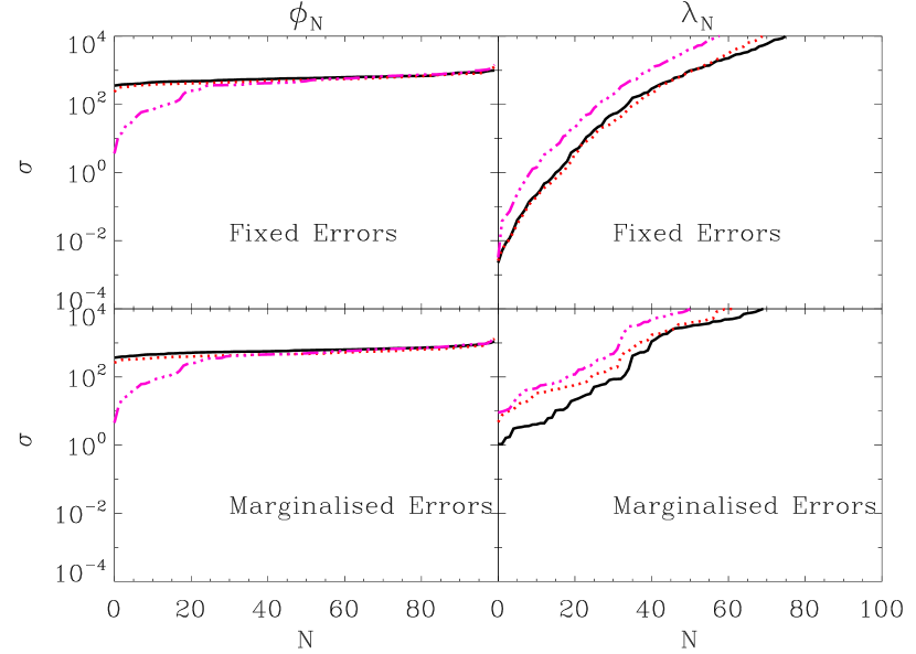
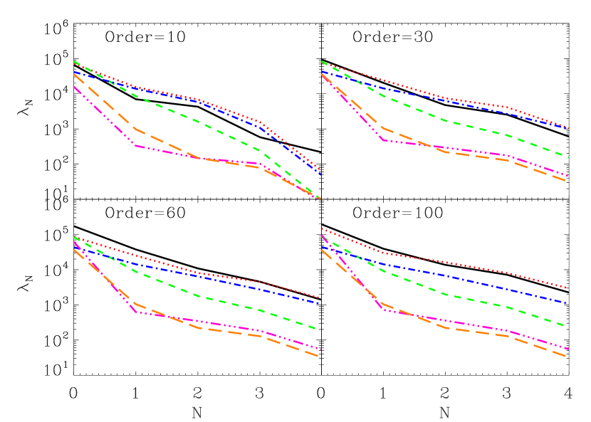
Figure 2 shows the expected $w(z)$ conditional errors on the original basis function coefficients and on the eigenfunctions. It can be seen that by rotating into an eigenbasis set the distribution of errors is skewed to produce more well defined functions as well as more poorly constrained functions in comparison to the non-rotated set.

It can be seen from the left panels of Figure 2 that the best constrained eigenfunctions have a similar error (the variance between the lines is small) but for the poorest constrained functions the variance between the basis sets is larger. This is because the most well constrained eigenfunctions are similar for each basis set whereas the poorest constrained have very different functional forms. As shown in Section 2.2 the set of eigenfunctions is not unique.

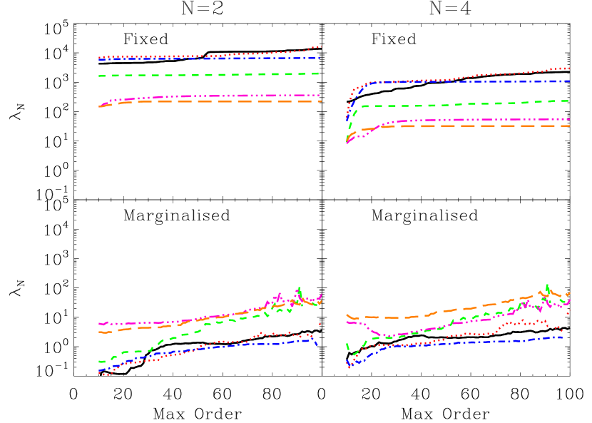
We also show the errors marginalised over the non-$w(z)$ parameters. For the eigenvalue case this is done using equation (2.3) where the eigenfunctions are the $w(z)$-only eigenfunctions. In all cases the best constrained eigenfunctions are those that are also the most degenerate with the other cosmological parameters, and marginalising over these can increase the error on the eigenfunctions by an order of magnitude.

Figure 3 shows how the largest $5$ eigenvalues change as a function of the maximum order in the expansion. It can be seen that a stable regime is found in which the values do not change substantially as the order is increased. We expand this in Figure 4 where we show how the eigenvalues for the second and fourth eigenfunctions change as a function of maximum order. The Fourier and Chebyshev values agree at higher order, the other basis sets – particularly interpolations and tophat – are very slow to converge. Even for a maximum order of $N=100$ there remains a large variance between the basis sets and that this variance increases as the eigenvalues decrease. The eigenvalues are related to the eigenfunction errors by $\sigma=1/\sqrt{\lambda}$, we show these errors in Figure 2. The best constrained $N=0$ eigenfunction has a similar error (for tophat, Chebyshev and Fourier basis sets) but by $N\geq 2$ the errors can vary by a factor $\mathrel{\raise 1.16pt\hbox{$>$}\kern-7.0pt\lower 3.06pt\hbox{{$\scriptstyle\sim$}}}10$.

There is a large range of eigenvalues between the basis sets, the most notable outliers being the tophat and interpolation basis sets. This is related to the fact that the residual, even at a maximum order of $100$, between the reconstructed eigenfunctions and the true eigenfunctions is significant. We investigate this further in Section 3.2. When we marginalise over the non-$w(z)$ parameters the variance between the basis sets remains but each basis set’s errors are effected in different ways since the basis functions are degenerate with the non-$w(z)$ parameters to different degrees.

We have performed a numerical test that checks that the eigendecomposition of the Fisher matrix is working correctly. First we find the eigenfunctions by diagonalising the $w(z)$ sub-Fisher matrix. We then use the eigenfunctions as a new basis set. We create a new Fisher matrix which takes derivatives with respect to the coefficients of the new (eigenbasis set). This new Fisher matrix should be diagonal and should have diagonal elements that are equal to the original Fisher matrice’s eigenvalues. We find that the code used in this article successfully passes this numerical check. The code used is available as part of iCosmo v$1.2$ and later.

3.2 Eigenfunctions

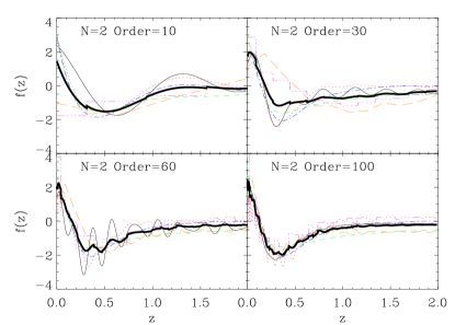
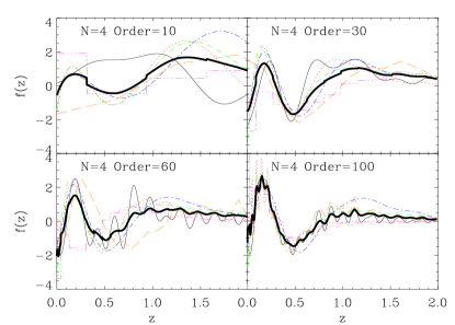
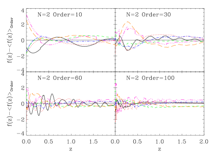
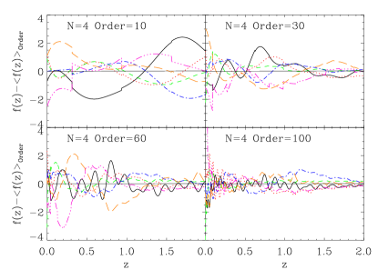
The eigenfunctions are reconstructed from the eigenmatrix $Q$ using equation (14). Figure 5 shows the second and fourth best constrained eigenfunctions for different maximum orders in the expansion for each basis set. In the absence of any way to reconstruct the ‘true’ eigenmatrix we also show the mean eigenfunction averaged over basis sets for each order – in the limit of a high order we expect the eigenfunctions to converge.

It can be seen that at ${\rm Order}=40$, for example, there is still a significant variation between basis sets. The variance between basis sets decreases as the maximum order is increased but for the $N=4$ function the tophat basis set varies significantly from the mean. We show the difference between each basis sets eigenfunction and the mean in Figure 6.

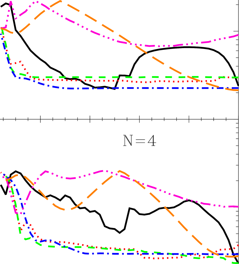
In Figure 7 we show the variance between the functions for a given basis set and order and the mean eigenfunctions for $N=100$. In general as the order increases the variance between the basis sets decreases. For some basis sets such as Chebyshev, Laguerre and Legendre polynomials there is already convergence even at a low order of $\sim 40$. At very low order $N\mathrel{\raise 1.16pt\hbox{$<$}\kern-7.0pt\lower 3.06pt\hbox{{$\scriptstyle\sim$}}}10$ the eigenfunctions are very noisy. Other basis sets such as Fourier and interpolation reach convergence at a high order $\sim 100$. The Fourier basis set is noisy since high order functions can introduce highly oscillatory modes into the eigenfunctions, this can also be seen in the $N=60$ panel in Figure 5. The tophat basis set requires an even higher order. We note that there would be even better agreement between the non-tophat basis sets and the mean if we excluded the tophat basis set from this analysis.

Figure 7: The variance between the eigenfunctions, reconstructed using a maximum order in the basis set expansion, and the mean eigen function using an order of $100$. The key to the different basis sets lines is given in Table 1. The upper panel shows the variance for the second best constrained eigenfunctions and the lower panel show the variance for the fourth best constrained eigen function.

4 Conclusion

We have found there is some ambiguity in the use of eigendecomposition in the literature to date and have aimed to clarify this situation. By investigating an arbitrary basis set expansion of $w(z)$ we have found that the technique of finding the eigenfunctions of $w(z)$ from the Fisher matrix is sensitive to the basis set choice and the order of the truncated expansion.

We used the example of a weak lensing tomographic survey to demonstrate how the eigenfunction decomposition is sensitive to these choices. We find that for a Euclid/DUNE-like survey the best constrained eigenfunctions could be determined to an accuracy of $\leq 1\%$ using lensing alone (no priors).

de Putter & Linder (2008) also presented a critique of the eigendecomposition approach which sheds further doubt on the technique’s validity, especially at low truncated order. They note that whilst the noise term on an eigenfunction can be predicted it is in fact the signal-to-noise that will be important for future surveys. We note then that a low order expansion in a particular basis set is not robust and also has uncertain relevance in gauging the predicted performance of a future survey.

Because of these ambiguities in the reconstruction of $w(z)$ we recommend a move towards using physically motivated functional forms based on models. Physical parameters can be constrained and models compared using evidence calculations (e.g. Trotta, 2007; Heavens et al., 2007 for a link with Fisher matrices).

We summarise our conclusions here

• The parameterisation of $w(z)$ is an arbitrary basis set choice, and since we do not know the nature of dark energy in general any choice is valid.

• When using orthogonal basis sets it is important to self-consistently include the weight function.

• When one refers to “binning” one is actually referring to a tophat basis set. Interpolation is also valid but should not be confused with binning.

• The set of eigenfunctions for a finite truncated basis set is not unique. There will always exists some eigenfunctions that are not common to all (truncated) eigenfunction sets.

• When different basis sets are truncated to high order the best constrained eigenfunctions will tend to agreement.

• When marginalising over extra cosmological parameters we show that finding the eigenfunctions of the full Fisher matrix leads to mixed non-$w(z)$ and $w(z)$ eigenfunctions that are dependent on the non-$w(z)$ parameterisation. We propose an alternative in which the marginalisation affects the $w(z)$ eigenvalues only, but not the functions themselves, by finding the eigenfunctions of the $w(z)$ sub-matrix.

• To find agreement between the top $\sim 4$ eigenfunctions an order of at least $100$ is required, for some basis set choices this is higher.

The convergence of the eigenfunctions depends on the original choice of basis sets – some converge more quickly than others. We find that Chebyshev, Legendre and Laguerre polynomials reach convergence more quickly than interpolation, tophat or Fourier basis sets.

Even with an order of $100$, the residuals between the reconstructed eigenfunctions cause the associated errors to vary by as much as a factor of $1$ – $10$ for the best $\sim 4$ constrained functions.

We note that the dark energy Figure of Merit suggested by Albrecht et al. (2009) uses a tophat basis set with $36$ parameters.

We recommend that if an eigenfunction Fisher matrix analysis is needed then a robust procedure should be followed with respect to marginalisation such that results are not affected by non-dark energy assumptions and priors and that a very high order of expansion is needed. The convergence can be tested by investigating a variety of basis sets – using only a single basis set is insufficient.

The code used in the article will form part of the iCosmo open source package and will be available in version $1.2$ at http://www.icosmo.org.

Appendix A Equivalence of eigen and Jacobian matrices

In this Appendix we will show that the eigenmatrix is equal to a Jacobian matrix. The eigenvalue decomposition of a matrix can be written like

$$Q\Lambda Q^{T}=F.$$ (24)

The Jacobian transform of a Fisher matrix maps from one parameter set $a_{i}$ to another $b_{i}$

$$J\Lambda J^{T}=F$$ (25)

where the matrix J in this case maps from the set $b$ to $a$. Where $\Lambda$ and $F$ are defined as

$$F_{ij}=\sum_{x}\left[\sigma^{-2}_{C}\frac{\partial C(\phi;x)}{\partial a_{i}}\frac{\partial C(\phi;x)}{\partial a_{j}}\right]$$

$$\Lambda_{ij}=\sum_{x}\left[\sigma^{-2}_{C}\frac{\partial C(\psi;x)}{\partial b_{i}}\frac{\partial C(\psi;x)}{\partial b_{j}}\right]$$

and the signal is parameterised in as

$$C(\phi;x)=\sum_{i}a_{i}\phi_{i}(x)$$

$$C(\psi;x)=\sum_{i}b_{i}\psi_{i}(x)$$ (27)

in $F$ and $\Lambda$ respectively. The elements of the Jacobian are

$$J_{ij}=\frac{\partial b_{j}}{\partial a_{i}}.$$ (28)

When transforming from one basis set to another we can write the following

$$a_{n} = \frac{1}{c_{n}}\int_{R}f(x)\phi_{n}(x)M(x){\rm d}x$$

$$= \frac{1}{c_{n}}\int_{R}\left(\sum_{m}b_{m}\psi_{m}(x)\right)\phi_{n}(x)M(x){\rm d}x$$

so that the Jacobian can be written

$$\frac{\partial a_{n}}{\partial b_{m}}=\frac{1}{c^{\phi}_{n}}\int_{R}\psi_{m}(x)\phi_{n}(x)M_{\phi}(x){\rm d}x$$ (30)

where the weight $M$ and constant $c$ are for the $\phi$ basis set.

If we assume that $\psi$ are eigenfunctions of the $\phi$ then they can be reconstructed using linear combinations of the original basis functions

$$\psi_{i}(x)=\sum_{j}Q_{ij}\phi_{j}(x).$$ (31)

Since the decomposition of a matrix $F$ to a diagonal matrix $\Lambda$ in equations (24) and equations (25) is unique it can easily be seen that the eigenmatrix is in fact a Jacobian. This can be shown in the following way. The Jacobian is written like

$$\frac{\partial a_{n}}{\partial b_{m}}=\frac{1}{c^{\phi}_{n}}\int_{R}\psi_{m}(x)\phi_{n}(x)M_{\phi}(x){\rm d}x.$$ (32)

We construct new basis sets as linear combinations of the old so that

$$\frac{\partial a_{n}}{\partial b_{m}}=\frac{1}{c^{\phi}_{n}}\int_{R}Q_{mk}\phi_{k}(x)\phi_{n}(x)M_{\phi}(x){\rm d}x$$ (33)

this leads to

$$\frac{\partial a_{n}}{\partial b_{m}} = \frac{1}{c^{\phi}_{n}}Q_{mk}\int_{R}\phi_{k}(x)\phi_{n}(x)M_{\phi}(x){\rm d}x$$

$$= \frac{1}{c^{\phi}_{n}}Q_{mk}\delta_{kn}c^{\phi}_{n}$$

$$J_{mn} = Q_{mn}.$$ (34)

Appendix B Non-uniqueness of the eigenvalues

Here we will show that if the residual between the reconstruction of a basis set using another is non-zero then the eigenvalues obtained from each set via an eigenvalue decomposition of the Fisher matrices are not equal.

The rotation matrix from basis $\phi$ to $\psi$ can be written

$$J_{ij}=\frac{1}{c^{\phi}}\int_{R}{\rm d}x\psi_{i}(x)\phi_{j}(x)M^{\phi}(x).$$ (35)

We now assume that the new basis functions can be written as the sum of some linear combination of the old basis functions plus some residual (equation 2.2)

$$J_{ij}=\frac{1}{c^{\phi}}\int_{R}{\rm d}x(J^{A}_{ik}\phi_{k}(x)+R_{i}(x))\phi_{j}(x)M^{\phi}(x)$$ (36)

where the rotation matrix $J^{A}$ rotates the old Fisher matrix to the new Fisher matrix assuming no residual. This can now be written like

$$J_{ij} = J^{A}_{ij}+T_{ij}$$

$$T_{ij} = \frac{1}{c^{\phi}}\int_{R}{\rm d}xR_{i}(x)\phi_{j}(x)M^{\phi}(x).$$ (37)

In the following we will use subscripts for the basis for clarity. We now rotate from $\phi$ to $\psi$ then diagonalise the Fisher matrix of $\psi$ to get $\Lambda_{\psi}$ this can be written as

$$J^{-1}_{\psi\Lambda_{\psi}}(J^{A}_{\phi\psi}+T_{\phi\psi})^{-1}F_{\phi\phi}(J^{A}_{\phi\psi}+T_{\phi\psi})J_{\psi\Lambda_{\psi}}=\Lambda_{\psi}.$$ (38)

We can also diagonalise $F_{\phi\phi}$ directly to get $\Lambda_{\phi}$

$$J^{-1}_{\phi\Lambda_{\phi}}F_{\phi\phi}J_{\phi\Lambda_{\phi}}=\Lambda_{\phi}.$$ (39)

If we assume that $\Lambda_{\psi}=\Lambda_{\phi}=\Lambda$ then comparing equations (38) and (39) the following must be true

$$(J^{A}_{\phi\psi}+T_{\phi\psi})J_{\psi\Lambda}=J_{\phi\Lambda}$$

$$J^{A}_{\phi\psi}J_{\psi\Lambda}+T_{\phi\psi}J_{\psi\Lambda}=J_{\phi\Lambda},$$ (40)

since we have assumed $\Lambda_{\psi}=\Lambda_{\phi}$ the first pair of rotation matrices commute (however in general this is not true) $J_{\phi\psi}J_{\psi\Lambda}=J_{\phi\Lambda}$ and we have

$$J_{\phi\Lambda}+T_{\phi\psi}J_{\psi\Lambda}=J_{\phi\Lambda}$$ (41)

which leads to

$$T_{\phi\psi}J_{\psi\Lambda}=0$$

$$T_{\phi\psi}=0.$$ (42)

So if $\Lambda_{\psi}=\Lambda_{\phi}$ then $T_{\psi\phi}=0$. By deduction we can then assert that if $T_{\psi\phi}\not=0$ then $\Lambda_{\psi}\not=\Lambda_{\phi}$ and the eigenvalues are not unique.

References

- [1] Albrecht A., et al., 2009, eprint arXiv:0901.0721
- [2] Albrecht A., Bernstein, G.; 2007, Phys.Rev.D, 75, 103003
- [3] Amara A., Refregier A., 2007, MNRAS, 381, 1018
- [4] Bagla J.S., Jassal H.K., Padmanabhan T.; 2003, Phys.Rev. D, 67, 063504
- [5] Chevallier, M.; Polarski, D.; 2001, IJMPD, 10, 213
- [6] Crittenden R., Pogosian L.; 2005, eprint astro.ph/0510293
- [7] Cunha C., Huterer D., Frieman J.; 2009, eprint arXiv:0904.1589
- [8] de Putter R., Linder E.; 2008, eprint arXiv:0812.1794
- [9] Dick J., Knox L., Chu M.; 2006, JCAP, 0607, 001
- [10] Heavens A., Kitching T., Verde L.; 2007, MNRAS, 380, 1029
- [11] Huterer D., Starkman G., 2003, PhRvL, 90, 1301
- [12] Huterer D., Cooray A.; 2005, Phys.Rev. D, 71, 023506
- [13] Hu W., 2002; 2002, Phys.Rev.D, 66, 083515
- [14] Ishak M., Upadhye A., Spergel D.; 2006, PhRvD, 74, 3513
- [15] Joudaki S., Cooray A., Holz D.; 2009 e-print arXiv:0904.4697
- [16] Kitching T., Amara A., Rassat A., Refregier A.; 2009, arXiv:0901.3143
- [17] Knox L., Albrecht A., Song Y.S.; 2005, ASPC, 339, 107
- [18] Refregier A., et al.; 2006, SPIE, 6265, 58
- [19] Refregier A., Amara A., Kitching T., Rassat A.; 2008, eprint arXiv0810.1285
- [20] Sarkar D., et al.; 2008, Phys. Rev. Lett. 100, 241302
- [21] Simpson F.; Bridle, S.; 2006, Phys.Rev. D, 73, 083001
- [22] Tang, J.; Abdalla, F. B.; Weller, J.; 2008, eprint arXiv:0807.3140
- [23] Tegmark, M.; Taylor A., Heavens A.; 1997, ApJ, 440, 22
- [24] Trotta R.; 2007, MNRAS, 378, 72
- [25] Zhan H., Knox L., Tyson J.; 2009a, ApJ, 690, 923
- [26] Zhan H. et al.; 2009b, eprint arXiv:0902.2599
- [27] Zhang F.; 2005, The Schur Complement and its Applications, Springer, 978-0387242712