thanks: E-mail: Bettina.Berg@uni-ulm.de.

Commuting Heisenberg operators as the quantum response problem:
Time-normal averages in the truncated Wigner representation.

B. Berg Institut für Quantenphysik, Universität Ulm, D-89069, Ulm, Germany.    L. I. Plimak Institut für Quantenphysik, Universität Ulm, D-89069, Ulm, Germany. ARC Centre of Excellence for Quantum-Atom Optics, School of Physical Sciences, University of Queensland, Brisbane, Qld 4072, Australia.    A. Polkovnikov Boston University, Department of Physics, Boston, MA, 02215, USA    M. K. Olsen Institut für Quantenphysik, Universität Ulm, D-89069, Ulm, Germany. ARC Centre of Excellence for Quantum-Atom Optics, School of Physical Sciences, University of Queensland, Brisbane, Qld 4072, Australia.    M. Fleischhauer Fachbereich Physik, Technische Universität Kaiserslautern, D-67633 Kaiserslautern, Germany.    W. P. Schleich Institut für Quantenphysik, Universität Ulm, D-89069, Ulm, Germany.
Abstract

The applicability of the so-called truncated Wigner approximation (–W) is extended to multitime averages of Heisenberg field operators. This task splits naturally in two. Firstly, what class of multitime averages the –W approximates, and, secondly, how to proceed if the average in question does not belong to this class. To answer the first question we develop an (in principle, exact) path-integral approach in phase-space based on the symmetric (Weyl) ordering of creation and annihilation operators. These techniques calculate a new class of averages which we call time-symmetric. The –W equations emerge as an approximation within this path-integral techniques. We then show that the answer to the second question is associated with response properties of the system. In fact, for two-time averages Kubo’s renowned formula relating the linear response function to two-time commutators suffices. The –W is trivially generalised to the response properties of the system allowing one to calculate approximate time-normally ordered two-time correlation functions with surprising ease. The techniques we develop are demonstrated for the Bose-Hubbard model.

pacs:
02.50.Ey,03.65.Sq,05.10.Gg

I Introduction

One of the most fascinating areas of ultra-cold atomic physics is the experimental investigation of the dynamical properties of interacting many-body systems. The control of experimental parameters and ability to tailor systems is allowing many interesting effects to be observed which would have been almost impossible in the recent past. Among important examples are the recently observed dynamical instabilities Fallani and inhibited transport Fertig ; mun in one dimensional (1D) and three-dimensional (3D) optical lattice systems, as well as nonlinear self-trapping in 1D periodic potentials Anker and in Josephson junctions Albiez . Despite these important experimental advances, the theoretical description of dynamical properties, especially for strong interactions, remains a major challenge, with progress having been incremental up to now. For bosons, except for rare cases where the dynamics are analytically tractable, e.g. by Bethe ansatz Caux , one method is to adapt the phase-space representations of quantum optics Glauber ; Sudarshan ; plusP ; GardinerQN . Attempts have been made, for example, to apply the positive-P representation to the dynamics of trapped and colliding Bose-Einstein condensates WBEC1 ; Joel ; jjhletter ; Deuar , although these have been only partially successful due to numerical instabilities which mean that integration is restricted to either short times or small interaction strengths. We note here that efforts are being made to extend the usefulness of this method gauge1 ; gauge2 ; gauge3 , with promising results for single-mode systems. For 1D systems numerical algorithms based on adaptive matrix-product decompositions of the state vector, such as the t-DMRG DMRG and the related TEBD algorithm TEBD , have recently been developed. They too are restricted however to short times or systems with slow entanglement growth.

For highly nonlinear underdamped systems such as trapped condensates, it is often easier to use the truncated Wigner approximation (-W) Wminus , with the main advantage being that it is numerically stable WBEC1 ; WBEC2 ; WBEC3 ; WBEC4 and simple to implement. The –W takes into account initial uncertainty between conjugate variables or initial quantum noise ap_twa , which is often necessary to trigger certain dynamical processes. This method was recently used to predict and explain several experiments in the context of interacting cold atom systems. As an example, using this method the damping of a dipolar motion of a 1D condensate in an optical lattice was first predicted in ref. pw and later results were qualitatively confirmed in experiment Fertig . This experiment was later simulated more accurately using a multi-band version of the –W Ruostekoski . In Refs. Bistritser ; Hutchinson the –W was used to analyze splitting or merging between elongated condensates, closely mimicking the situation realized in recent experiments joerg1 . In Ref. psg , the –W enabled the authors to explain the coherence dynamics after a sudden quench of tunneling from an insulator to a superfluid, giving good agreement with experimental results ari . For a fuller review of other recent developments, we direct the reader to Ref. blakie .

While the truncated Wigner representation is becoming increasingly utilized, there are two drawbacks which prevent it from being the numerical technique of choice. The first is its approximate nature, arising from the truncation procedure, which may sometimes lead to demonstrably wrong results Wigwrong1 ; Wigwrong2 . In principle, this drawback can be overcome. A way to fully map the quantum master equation onto Wigner representation stochastic difference equations has been developed, but does not result in a widely and easily applicable method nossoEPL ; ourpreprint ; spontaneous . An expansion allowing one to include the dropped contribution perturbatively via quantum jumps was suggested in Ref. ap_twa , but until now this has been restricted to the calculation of single-time averages.

The second drawback is that averages of the phase-space variables in the Wigner representation do not map directly onto expectation values of time-normally ordered multitime operator products corresponding with experimental measurements. For two operators, we recover a symmetrised product, while for three and more operators, there emerges a new type of ordering of Heisenberg operators which we term time-symmetric ourpreprint . Converting these to time-normal ordering requires the calculation of commutators of Heisenberg operators at different times. At first glance this drawback appears to be fundamental, but we will demonstrate that it can be circumvented with surprising ease, by making use of the fact that commutators of Heisenberg operators at different times express the response properties of a quantum system ourpreprint ; Kubo1 ; Kubo2 ; Corr ; BWO ; PlSt . Generally, commuting the Heisenberg operators requires solving the full quantum stochastic nonlinear response problem, and, although possible in principle, this remains a formidable task PlSt ; Unpb . For two-time commutators, however, the process is simplified due to Kubo’s linear response formulation Kubo1 ; Kubo2 , which has previously been used to convert normally-ordered correlations into symmetrically ordered ones within the positive-P representation Wigwrong2 ; QNDBWO . In this paper we show how, combined with the truncated Wigner representation as a computational tool, Kubo’s linear response theory turns into a simple yet powerful approximate method of calculating two-time correlation functions of interacting bosonic fields with arbitrary operator ordering. We stress here that the Kubo relation is exact, with the approximate nature coming from the truncation process used to find the appropriate stochastic equations.

In more traditional phase-space techniques, the truncated-Wigner equations are developed by dropping the third-order derivatives in the generalised Fokker-Planck equation for the single-time Wigner distribution GardinerQN ; Wminus . The corresponding Langevin equations are either non-stochastic (without losses) or probabilistic (with losses) and are very easy to handle numerically. However simple and straightforward, this conventional way of deriving the truncated Wigner approach leaves it unclear if it can be applied to any multitime quantum averages. In our approach, the truncated-Wigner equations emerge as an approximation within rigorous phase-space path-integral techniques. By itself, the path integral expresses the averages of time-symmetrically-ordered products of Heisenberg operators. The generalisation associated with extending the truncated-Wigner equations to multitime averages is thus highly nontrivial and requires a new concept: the time-symmetric ordering of the Heisenberg operators. There does not seem to be a way of guessing this concept from within the conventional phase-space techniques. Just proving the equivalence between the time-symmetric and the conventional symmetric ordering of free-field operators is a nontrivial task Unpb .

To make this paper more accessible we will begin with a theoretical summary in section II, where we list the key results, supporting them by leading considerations. The actual theory is presented in section III. Sections IV and V illustrate how to apply the method in practice. The summary of section II suffices for understanding the examples in sections IV and V. The reader who is not interested in a rigorous justification of the method can safely ignore it. Our first example is Kerr oscillator (section IV). This is an exactly soluble problem; moreover, all calculations in the truncated Wigner approach can be carried out analytically. In section V we apply the method to the Bose-Hubbard model, comparing the results to direct calculations in Hilbert space. We consider relatively small chains consisting of few sites to make exact calculations possible, although the truncated Wigner approach can be extended to much larger systems (see e.g. Refs. ap_cat ; adiabatic ). We find good agreement between exact and approximate results over relatively short time scales, with the applicability of this method to longer times remaining an open problem.

II Theoretical summary

II.1 Symmetric representation of Heisenberg operators

We will assume that the reader is familiar with the phase-space basics, including the concepts of symmetric (Weyl’s) operator ordering, symmetric representation of operators and the Wigner function. The necessary minimum of information is summarised in section III.2. Details may be found in Refs. MandelWolf ; walls-milburn ; gardiner-zoller ; AgarwalWolf .

The formal techniques we develop in this paper extend the well-known symmetric representation of quantum optics GardinerQN to multitime problems. First and foremost, in place of a quasiaverage over the Wigner quasiprobability distribution we find a phase-space path integral. Within the path-integral techniques, we derive generalised phase-space correspondenses mapping multiplication of a q-number quantity by a creation or annihilation operator to phase-space. Conventional phase-space correspondenses apply to free operators and the generalised ones apply to Heisenberg operators. They are exact and do not depend on the nature of nonlinearity (interaction). Similarly to the way in which conventional phase-space correspondences allow one to reorder creation and annihilation operators, the generalised ones allow one to reorder a pair (say) of Heisenberg operators with unequal time arguments. These techniques are not restricted to any special Hamiltonian and can be employed for all bosonic systems.

To be specific, consider an illustrative example of the anharmonic oscillator (Kerr oscillator) with the Hamiltonian

H^0=κ2a^2a^2.subscript^𝐻0Planck-constant-over-2-pi𝜅2superscript^𝑎absent2superscript^𝑎2\displaystyle{{\begin{aligned} \hat{H}_{0}=\frac{\hbar\kappa}{2}\hat{a}^{\dagger 2}\hat{a}^{2}.\end{aligned}}} (1)

Here, a^,a^^𝑎superscript^𝑎\hat{a},\hat{a}^{{\dagger}} is the standard creation/annihilation pair,

[a^,a^]=1.^𝑎superscript^𝑎1\displaystyle{{\begin{aligned} \big{[}\hat{a},\hat{a}^{{\dagger}}\big{]}=1.\end{aligned}}} (2)

The Heisenberg “field operators” are defined in the normal manner as

𝒜^(t)=𝒰^(t,t0)a^𝒰^(t,t0),𝒜^(t)=𝒰^(t,t0)a^𝒰^(t,t0).formulae-sequence^𝒜𝑡superscript^𝒰𝑡subscript𝑡0^𝑎^𝒰𝑡subscript𝑡0superscript^𝒜𝑡superscript^𝒰𝑡subscript𝑡0superscript^𝑎^𝒰𝑡subscript𝑡0\displaystyle{{\begin{gathered}{\hat{\mathcal{A}}}(t)={\hat{\mathcal{U}}}^{\dagger}(t,t_{0})\hat{a}{\hat{\mathcal{U}}}(t,t_{0}),\\ {\hat{\mathcal{A}}}^{\dagger}(t)={\hat{\mathcal{U}}}^{\dagger}(t,t_{0})\hat{a}^{\dagger}{\hat{\mathcal{U}}}(t,t_{0}).\end{gathered}}} (5)

Here, 𝒰^(t,t0)^𝒰𝑡subscript𝑡0{\hat{\mathcal{U}}}(t,t_{0}) is the evolution operator, where t0subscript𝑡0t_{0} is the coincidence point for the Schrödinger and Heisenberg pictures. For an arbitrary H^0subscript^𝐻0\hat{H}_{0} the evolution operator is introduced through the Schrödinger equation,

i𝒰^(t,t0)t=H^0𝒰^(t,t0),𝒰^(t0,t0)=𝟙^.formulae-sequence𝑖Planck-constant-over-2-pi^𝒰𝑡subscript𝑡0𝑡subscript^𝐻0^𝒰𝑡subscript𝑡0^𝒰subscript𝑡0subscript𝑡0^𝟙\displaystyle{{\begin{aligned} i\hbar\frac{\partial{\hat{\mathcal{U}}}(t,t_{0})}{\partial t}=\hat{H}_{0}{\hat{\mathcal{U}}}(t,t_{0}),\ \ {\hat{\mathcal{U}}}(t_{0},t_{0})=\hat{\openone}.\end{aligned}}} (6)

Note that we do not divide the Hamiltonian into the free and interaction part, nor introduce the interaction picture, nor free-field operators. The methods we develop in this paper are strictly nonperturbative. The truncated Wigner representation does not correspond to linearisation of any kind. It follows separation of nonlinearity and noise for path-integral trajectories with neglecting the latter, for details see section III.4. There does not seem to be a way of even formulating such approximations in Hilbert-space terms.

In section III we construct a phase-space path-integral approach which allows one to calculate the quantum average of the symmetrised product

𝒯W𝒜^(t2)𝒜^(t1)=α(t1)α(t2)¯¯,delimited-⟨⟩subscript𝒯𝑊superscript^𝒜subscript𝑡2^𝒜subscript𝑡1¯¯𝛼subscript𝑡1superscript𝛼subscript𝑡2\displaystyle{{\begin{aligned} \big{\langle}{\cal T}_{W}\!{\hat{\mathcal{A}}}^{{\dagger}}(t_{2}){\hat{\mathcal{A}}}(t_{1})\big{\rangle}=\overline{\overline{\hskip 0.43057pt\alpha(t_{1})\alpha^{*}(t_{2})\hskip 0.43057pt}},\end{aligned}}} (7)

where For the time being, 𝒯Wsubscript𝒯𝑊{\cal T}_{W}\! is just an ad hoc notation; its actual meaning will be the subject of section II.3. The quantum averaging is over the Heisenberg ρ𝜌\rho-matrix ρ^^𝜌\hat{\rho}, (with 𝒳^^𝒳{\hat{\mathcal{X}}} being an arbitrary operator)

𝒳^=Trρ^𝒳^.delimited-⟨⟩^𝒳Tr^𝜌^𝒳\displaystyle{{\begin{aligned} \big{\langle}{\hat{\mathcal{X}}}\big{\rangle}=\text{Tr}\hat{\rho}{\hat{\mathcal{X}}}.\end{aligned}}} (8)

The double bar denotes symbolically the path integral over the c-number trajectories α(t)𝛼𝑡\alpha(t). It can be thought of as a stochastic average with a nonpositive “measure”, whose exact meaning will be clarified in the next section. What is important is that the path integral (7) is approximated by the truncated Wigner approach. In this approximation the trajectories α(t)𝛼𝑡\alpha(t) are deterministic and obey the equation

idα(t)dt=κ[|α(t)|21]α(t).𝑖𝑑𝛼𝑡𝑑𝑡𝜅delimited-[]superscript𝛼𝑡21𝛼𝑡\displaystyle{{\begin{aligned} i\frac{d\alpha(t)}{dt}=\kappa[|\alpha(t)|^{2}-1]\alpha(t).\end{aligned}}} (9)

This equation follows both from the traditional phase-space methods Wminus and from the path-integral techniques in section III. The trajectories being deterministic, stochasticity in Eq. ( 7) reduces to the averaging over the Wigner function W(α)𝑊𝛼W(\alpha) corresponding to the Heisenberg ρ𝜌\rho-matrix (assuming this function is nonnegative, W(α)0𝑊𝛼0W(\alpha)\geq 0). The path integral in Eq. ( 7) then reduces to averaging over solutions of Eq. ( 9) with a random initial condition,

α(t1)α(t2)¯=d2απW(α)α(t1)α(t2),¯𝛼subscript𝑡1superscript𝛼subscript𝑡2superscript𝑑2𝛼𝜋𝑊𝛼𝛼subscript𝑡1superscript𝛼subscript𝑡2\displaystyle{{\begin{aligned} \overline{\hskip 0.43057pt\alpha(t_{1})\alpha^{*}(t_{2})\hskip 0.43057pt}=\int\frac{d^{2}\alpha}{\pi}W(\alpha)\alpha(t_{1})\alpha^{*}(t_{2}),\end{aligned}}} (10)

where α(t)𝛼𝑡\alpha(t) is a solution to (15) with the initial condition α(t0)=α𝛼subscript𝑡0𝛼\alpha(t_{0})=\alpha. Making trajectories deterministic is an approximation, so that the average (10) only approximates the quantum average,

𝒯W𝒜^(t2)𝒜^(t1)α(t1)α(t2)¯,delimited-⟨⟩subscript𝒯𝑊superscript^𝒜subscript𝑡2^𝒜subscript𝑡1¯𝛼subscript𝑡1superscript𝛼subscript𝑡2\displaystyle{{\begin{aligned} \big{\langle}{\cal T}_{W}\!{\hat{\mathcal{A}}}^{{\dagger}}(t_{2}){\hat{\mathcal{A}}}(t_{1})\big{\rangle}\approx\overline{\hskip 0.43057pt\alpha(t_{1})\alpha^{*}(t_{2})\hskip 0.43057pt},\end{aligned}}} (11)

unlike the path integral (7) which is exact.

It is worth stressing here that the results of this paper are not Eqs. ( 9)–(11) as such, but the fact that they apply with t1t2subscript𝑡1subscript𝑡2t_{1}\neq t_{2}. The truncated Wigner approach was derived within the conventional phase-space techniques. By construction, it is only applicable to time-dependent averages of Schrödinger operators, or, equivalently, to averages of Heisenberg operators with equal time arguments. In other words, conventional phase-space methods allow one to verify Eqs. ( 9)–(11) only for t1=t2subscript𝑡1subscript𝑡2t_{1}=t_{2}. Extension to unequal times (physically, to spectral properties of the system) requires alternative techniques such as a phase-space path integral.

II.2 Generalised phase-space correspondences

Our next goal is to extend the truncated-Wigner further by lifting the ordering restriction of Eq. ( 7). Namely, we wish to calculate the time-normally ordered average,

𝒜^(t1)𝒜^(t2)=𝒯W𝒜^(t2)𝒜^(t1)12[𝒜^(t2),𝒜^(t1)],delimited-⟨⟩superscript^𝒜subscript𝑡1^𝒜subscript𝑡2delimited-⟨⟩subscript𝒯𝑊superscript^𝒜subscript𝑡2^𝒜subscript𝑡112delimited-⟨⟩^𝒜subscript𝑡2superscript^𝒜subscript𝑡1\hskip 86.72267pt\big{\langle}\hat{\cal A}^{\dagger}(t_{1})\hat{\cal A}(t_{2})\big{\rangle}=\big{\langle}{\cal T}_{W}\!{\hat{\mathcal{A}}}^{{\dagger}}(t_{2}){\hat{\mathcal{A}}}(t_{1})\big{\rangle}\\ -\frac{1}{2}\big{\langle}\big{[}\hat{\cal A}(t_{2}),\hat{\cal A}^{\dagger}(t_{1})\big{]}\big{\rangle},\hskip 86.72267pt (12)

where it has been expressed by the symmetrised average and the commutator. The symmetrised term is given by (7). To express the commutator we employ the same idea as was used in Ref. QNDBWO to reorder a time-normal average symmetrically. Namely, we assume that t2>t1subscript𝑡2subscript𝑡1t_{2}>t_{1} and relate the commutator to the linear response of the system,

[𝒜^(t2),𝒜^(t1)]=iδ𝒜^(t2)δs(t1)|s=0.delimited-⟨⟩^𝒜subscript𝑡2superscript^𝒜subscript𝑡1evaluated-at𝑖Planck-constant-over-2-pi𝛿delimited-⟨⟩^𝒜subscript𝑡2𝛿𝑠subscript𝑡1𝑠0\displaystyle{{\begin{aligned} \big{\langle}\big{[}{\hat{\mathcal{A}}}(t_{2}),{\hat{\mathcal{A}}}^{{\dagger}}(t_{1})\big{]}\big{\rangle}=-i\hbar\frac{\delta\big{\langle}{\hat{\mathcal{A}}}(t_{2})\big{\rangle}}{\delta s(t_{1})}\bigg{|}_{s=0}.\end{aligned}}} (13)

This relation is simply Kubo’s formula for the linear response function Kubo1 ; Kubo2 written “from right to left.” It implies that the Hamiltonian of the system has been complemented by an interaction with the external c-number source s(t)𝑠𝑡s(t),

H^0H^(t)=H^0s(t)a^s(t)a^.subscript^𝐻0^𝐻𝑡subscript^𝐻0𝑠𝑡superscript^𝑎superscript𝑠𝑡^𝑎\displaystyle{{\begin{aligned} \hat{H}_{0}\to\hat{H}(t)=\hat{H}_{0}-s(t)\hat{a}^{{\dagger}}-s^{*}(t)\hat{a}.\end{aligned}}} (14)

Strictly speaking, the condition s=0𝑠0s=0 must then be applied to both sides of Eq. ( 13) (and in fact to all quantum averages in the above), but in practice it suffices to remember that the only quantity defined with s0𝑠0s\neq 0 is 𝒜^(t2)delimited-⟨⟩^𝒜subscript𝑡2\big{\langle}{\hat{\mathcal{A}}}(t_{2})\big{\rangle} in Eq. ( 13).

For simplicity we will confine the rest of the discussion to the truncated Wigner representation. In this case the trajectories α(t)𝛼𝑡\alpha(t) are deterministic and obey the equation which differs from (9) by the presence of an additive source:

idα(t)dt=κ[|α(t)|21]α(t)s(t).𝑖𝑑𝛼𝑡𝑑𝑡𝜅delimited-[]superscript𝛼𝑡21𝛼𝑡𝑠𝑡\displaystyle{{\begin{aligned} i\frac{d\alpha(t)}{dt}=\kappa[|\alpha(t)|^{2}-1]\alpha(t)-s(t).\end{aligned}}} (15)

Within conventional phase-space methods, we find this equation by noting that the linear interaction terms in the Hamiltonian contribute only to drift terms in the generalised Fokker-Planck equation. A path-integral derivation of (15) extending its applicability to multitime averages will be given in section III.4.

To calculate the linear response function (14) one needs an infinitesimal instantaneous source at t=t1𝑡subscript𝑡1t=t_{1},

s(t)=iδαδ(tt1).𝑠𝑡𝑖Planck-constant-over-2-pi𝛿𝛼𝛿𝑡subscript𝑡1\displaystyle{{\begin{aligned} s(t)=-i\hbar\,\delta\alpha\,\delta(t-t_{1}).\end{aligned}}} (16)

Substituting this source into Eq. ( 15) we see that it causes a discontinuity of the trajectory at t=t1𝑡subscript𝑡1t=t_{1} (a “quantum jump” in the terminology of Ref. ap_twa ). The additional factors in (16) were chosen so as to make this discontinuity exactly equal to δα𝛿𝛼\delta\alpha. We thus have a simple correspondence between sources and “quantum jumps”:

δδs(t1)iα(t1),δδs(t1)iα(t1).missing-subexpression𝛿𝛿𝑠subscript𝑡1𝑖Planck-constant-over-2-pi𝛼subscript𝑡1𝛿𝛿superscript𝑠subscript𝑡1𝑖Planck-constant-over-2-pisuperscript𝛼subscript𝑡1\displaystyle{{\begin{aligned} &\frac{\delta}{\delta s(t_{1})}\Longleftrightarrow\frac{i}{\hbar}\frac{\partial}{\partial\alpha(t_{1})},&\frac{\delta}{\delta s^{*}(t_{1})}\Longleftrightarrow-\frac{i}{\hbar}\frac{\partial}{\partial\alpha^{*}(t_{1})}.\end{aligned}}} (17)

Mathematically, the derivatives /α(t1),/α(t1)𝛼subscript𝑡1superscript𝛼subscript𝑡1{\partial}/{\partial\alpha(t_{1})},{\partial}/{\partial\alpha^{*}(t_{1})} correspond to a variation of the initial condition set at t=t1𝑡subscript𝑡1t=t_{1} instead of t=t0𝑡subscript𝑡0t=t_{0}. Such notation is to some extent informal but convenient. For the commutator we then find (t1<t2subscript𝑡1subscript𝑡2t_{1}<t_{2})

[𝒜^(t2),𝒜^(t1)]=α(t2)α(t1)¯,t2>t1.formulae-sequencedelimited-⟨⟩^𝒜subscript𝑡2superscript^𝒜subscript𝑡1¯𝛼subscript𝑡2𝛼subscript𝑡1subscript𝑡2subscript𝑡1\displaystyle{{\begin{aligned} \big{\langle}\big{[}\hat{\cal A}(t_{2}),\hat{\cal A}^{\dagger}(t_{1})\big{]}\big{\rangle}=\overline{\frac{\partial\alpha(t_{2})}{\partial\alpha(t_{1})}},\ \ t_{2}>t_{1}.\end{aligned}}} (18)

This relation follows from the correspondences (17) and from the path-integral representation of the average.

𝒜^(t2)=α(t2)¯.delimited-⟨⟩^𝒜subscript𝑡2¯𝛼subscript𝑡2\displaystyle{{\begin{aligned} \big{\langle}\hat{\cal A}(t_{2})\big{\rangle}=\overline{\alpha(t_{2})}.\end{aligned}}} (19)

Using (18) we can express the time-normal average in the Wigner representation,

𝒜^(t1)𝒜^(t2){α(t1)α(t2)12α(t2)α(t1)¯,t1<t2,α(t1)α(t2)12[α(t1)α(t2)]¯,t1>t2.delimited-⟨⟩superscript^𝒜subscript𝑡1^𝒜subscript𝑡2cases¯superscript𝛼subscript𝑡1𝛼subscript𝑡212𝛼subscript𝑡2𝛼subscript𝑡1subscript𝑡1subscript𝑡2¯superscript𝛼subscript𝑡1𝛼subscript𝑡212superscriptdelimited-[]𝛼subscript𝑡1𝛼subscript𝑡2subscript𝑡1subscript𝑡2\displaystyle{{\begin{aligned} \big{\langle}\hat{\cal A}^{\dagger}(t_{1})\hat{\cal A}(t_{2})\big{\rangle}\approx\left\{\begin{array}[]{ll}\overline{\alpha^{*}(t_{1})\alpha(t_{2})-\displaystyle\frac{1}{2}\frac{\partial{\alpha(t_{2})}}{\partial\alpha(t_{1})}},&t_{1}<t_{2},\\ \displaystyle\overline{\alpha^{*}(t_{1})\alpha(t_{2})-\frac{1}{2}\bigg{[}\frac{\partial{\alpha(t_{1})}}{\partial\alpha(t_{2})}\bigg{]}^{*}},&t_{1}>t_{2}\,.\end{array}\right.\end{aligned}}} (20)

The second line here follows by conjugating the first one and replacing t1t2subscript𝑡1subscript𝑡2t_{1}\leftrightarrow t_{2}.

These generalised phase-space correspondences (20) are the central result of the paper. Certainly, the above derivation is no more than leading considerations, but the rigorous treatment in section III.6 gives the same result. Moreover, it shows that Eqs. ( 20) hold not only as an approximation in the truncated Wigner representation, but also as an exact relation within the rigorous path-integral approach — in which case the bar in (20) should be replaced by double bar.

Why do we call Eqs. ( 20) “generalised phase-space correspondences?” To recognise the connection we take the limit t1,t2t0subscript𝑡1subscript𝑡2subscript𝑡0t_{1},t_{2}\to t_{0}. Using the fact that that 𝒜^(t0)=a^,𝒜^(t0)=a^formulae-sequence^𝒜subscript𝑡0^𝑎superscript^𝒜subscript𝑡0superscript^𝑎\hat{\cal A}(t_{0})=\hat{a},\hat{\cal A}^{\dagger}(t_{0})=\hat{a}^{{\dagger}} and dropping the time argument in α(t0)𝛼subscript𝑡0\alpha(t_{0}) we find

a^a^=(α12α)α¯=(α12α)α¯,delimited-⟨⟩superscript^𝑎^𝑎¯𝛼12superscript𝛼superscript𝛼¯superscript𝛼12𝛼𝛼\displaystyle{{\begin{aligned} \big{\langle}\hat{a}^{{\dagger}}\hat{a}\big{\rangle}=\overline{\hskip 0.43057pt\bigg{(}\alpha-\frac{1}{2}\frac{\partial}{\partial\alpha^{*}}\bigg{)}\alpha^{*}\hskip 0.43057pt}=\overline{\hskip 0.43057pt\bigg{(}\alpha^{*}-\frac{1}{2}\frac{\partial}{\partial\alpha}\bigg{)}\alpha\hskip 0.43057pt},\end{aligned}}} (21)

where the averaging is simply over the Wigner function W(α)𝑊𝛼W(\alpha), cf. Eq. ( 10). First of all, both relations in Eq. ( 21) are correct. Indeed, they result in the formula

a^a^=|α|2¯12.delimited-⟨⟩superscript^𝑎^𝑎¯superscript𝛼212\displaystyle{{\begin{aligned} \big{\langle}\hat{a}^{{\dagger}}\hat{a}\big{\rangle}=\overline{\hskip 0.43057pt|\alpha|^{2}\hskip 0.43057pt}-\frac{1}{2}\,.\end{aligned}}} (22)

The average over the Wigner function expresses symmetrically ordered products of a^,a^^𝑎superscript^𝑎\hat{a},\hat{a}^{{\dagger}}; in particular,

|α|2¯=12a^a^+a^a^=a^a^+12,¯superscript𝛼212delimited-⟨⟩^𝑎superscript^𝑎superscript^𝑎^𝑎delimited-⟨⟩superscript^𝑎^𝑎12\displaystyle{{\begin{aligned} \overline{\hskip 0.43057pt|\alpha|^{2}\hskip 0.43057pt}=\frac{1}{2}\big{\langle}\hat{a}\hat{a}^{{\dagger}}+\hat{a}^{{\dagger}}\hat{a}\big{\rangle}=\big{\langle}\hat{a}^{{\dagger}}\hat{a}\big{\rangle}+\frac{1}{2},\end{aligned}}} (23)

in obvious agreement with (22). Furthermore, Eqs. ( 21) are particular cases of the standard phase-space correspondences,

Y^a^=(α12α)Y(α)¯,delimited-⟨⟩^𝑌^𝑎¯𝛼12superscript𝛼𝑌𝛼\displaystyle{\begin{aligned} \Big{\langle}{\hat{Y}\hat{a}}\Big{\rangle}=\overline{\hskip 0.43057pt\bigg{(}\alpha-\frac{1}{2}\frac{\partial}{\partial\alpha^{*}}\bigg{)}Y(\alpha)\hskip 0.43057pt},\end{aligned}} (24)
a^Y^=(α12α)Y(α)¯,delimited-⟨⟩superscript^𝑎^𝑌¯superscript𝛼12𝛼𝑌𝛼\displaystyle{\begin{aligned} \Big{\langle}{\hat{a}^{{\dagger}}\hat{Y}}\Big{\rangle}=\overline{\hskip 0.43057pt\bigg{(}\alpha^{*}-\frac{1}{2}\frac{\partial}{\partial\alpha}\bigg{)}Y(\alpha)\hskip 0.43057pt},\end{aligned}} (25)

where Y^^𝑌\hat{Y} is an operator and Y(α)𝑌𝛼Y(\alpha) is its symmetric representation. The first of Eqs. ( 21) follows from Eq. ( 24) with Y^=a^,Y(α)=αformulae-sequence^𝑌superscript^𝑎𝑌𝛼superscript𝛼\hat{Y}=\hat{a}^{{\dagger}},Y(\alpha)=\alpha^{*}, and the second one — from Eq. ( 25) with Y^=a^,Y(α)=αformulae-sequence^𝑌^𝑎𝑌𝛼𝛼\hat{Y}=\hat{a},Y(\alpha)=\alpha. Multitime generalisations of Eqs. ( 24), (25) are derived in section III.6.

We conclude this paragraph with a remark on terminology. To maintain rigor, one should distinguish shifts of trajectories effected by instantaneous sources (16) from quantum jumps. The latter term was introduced in Ref. ap_twa , where discontinuities of trajectories were used as formal means to express perturbative corrections to the truncated Wigner approach. These corrections come from quantum noises which do not have any classical interpretation whatsoever, while the c-number external source is to a large extent a classical object. Maintaining the distinction between shifts and quantum jumps thus appears physically justified. However, such clear-cut distinction is an artifact of an undamped model with quartic interaction. For instance, for the damped harmonic oscillator the equation for the Wigner function is a genuine Fokker-Planck equation. In this case the “quantum noise” is fully probabilistic, i.e., classical. We will use “quantum jump” as a blanket term applicable to both types of discontinuities.

II.3 The time-symmetric ordering

The fact that the path integral (7) calculates (and the truncated Wigner approach approximates) symmetrised products of Heisenberg operators does not generalise to products of three and more operators. Instead of fully symmetrised products, one discovers a new type of ordering of Heisenberg operators, which we call time-symmetric and denote as 𝒯Wsubscript𝒯𝑊{\cal T}_{W}\!. We find this interesting and important enough to be worth reporting, notwithstanding the fact that it is not directly relevant to purposes of this paper.

A time-symmetrically ordered product of the “field operators” 𝒜^(t),𝒜^(t)^𝒜𝑡superscript^𝒜𝑡{\hat{\mathcal{A}}}(t),{\hat{\mathcal{A}}}^{{\dagger}}(t) is defined recursively as

𝒯W𝟙^=𝟙^,𝒯W𝒜^(t)=𝒜^(t),𝒯W𝒜^(t)=𝒜^(t),𝒯W𝒜^(t)𝒫^[>t]=12{𝒜^(t),𝒯W𝒫^[>t]},𝒯W𝒜^(t)𝒫^[>t]=12{𝒜^(t),𝒯W𝒫^[>t]}.missing-subexpressionformulae-sequencesubscript𝒯𝑊^𝟙^𝟙formulae-sequencesubscript𝒯𝑊^𝒜𝑡^𝒜𝑡subscript𝒯𝑊superscript^𝒜𝑡superscript^𝒜𝑡missing-subexpressionsubscript𝒯𝑊^𝒜𝑡subscript^𝒫delimited-[]absent𝑡12^𝒜𝑡subscript𝒯𝑊subscript^𝒫delimited-[]absent𝑡missing-subexpressionsubscript𝒯𝑊superscript^𝒜𝑡subscript^𝒫delimited-[]absent𝑡12superscript^𝒜𝑡subscript𝒯𝑊subscript^𝒫delimited-[]absent𝑡\displaystyle{{\begin{aligned} &{\cal T}_{W}\!\hat{\openone}=\hat{\openone},\ \ {\cal T}_{W}\!{\hat{\mathcal{A}}}(t)={\hat{\mathcal{A}}}(t),\ \ {\cal T}_{W}\!{\hat{\mathcal{A}}}^{{\dagger}}(t)={\hat{\mathcal{A}}}^{{\dagger}}(t),\\ &{\cal T}_{W}\!{\hat{\mathcal{A}}}(t){\hat{\mathcal{P}}}_{[>t]}=\frac{1}{2}\big{\{}{\hat{\mathcal{A}}}(t),{\cal T}_{W}\!{\hat{\mathcal{P}}}_{[>t]}\big{\}},\\ &{\cal T}_{W}\!{\hat{\mathcal{A}}}^{{\dagger}}(t){\hat{\mathcal{P}}}_{[>t]}=\frac{1}{2}\big{\{}{\hat{\mathcal{A}}}^{{\dagger}}(t),{\cal T}_{W}\!{\hat{\mathcal{P}}}_{[>t]}\big{\}}.\end{aligned}}} (26)

Here, 𝒫^[>t]subscript^𝒫delimited-[]absent𝑡{\hat{\mathcal{P}}}_{[>t]} is a product of field operators with all time arguments exceeding t𝑡t; the curly brackets stand for the anticommutator, {𝒳^,𝒴^}=𝒳^𝒴^+𝒴^𝒳^^𝒳^𝒴^𝒳^𝒴^𝒴^𝒳\{{\hat{\mathcal{X}}},{\hat{\mathcal{Y}}}\}={\hat{\mathcal{X}}}{\hat{\mathcal{Y}}}+{\hat{\mathcal{Y}}}{\hat{\mathcal{X}}}. It is implied that under the sign of 𝒯Wsubscript𝒯𝑊{\cal T}_{W}\!-ordering the field operators commute freely. The quantum average of an arbitrary time-symmetric product is expressed as a path-integral average, (m,n0𝑚𝑛0m,n\geq 0)

𝒯W𝒜^(t1)𝒜^(tm)𝒜^(t1)𝒜^(tn)=α(t1)α(tm)α(t1)α(tn)¯¯.delimited-⟨⟩subscript𝒯𝑊^𝒜subscript𝑡1^𝒜subscript𝑡𝑚superscript^𝒜subscriptsuperscript𝑡1superscript^𝒜subscriptsuperscript𝑡𝑛¯¯𝛼subscript𝑡1𝛼subscript𝑡𝑚superscript𝛼subscriptsuperscript𝑡1superscript𝛼subscriptsuperscript𝑡𝑛\hskip 86.72267pt\big{\langle}{\cal T}_{W}\!{\hat{\mathcal{A}}}(t_{1})\cdots{\hat{\mathcal{A}}}(t_{m}){\hat{\mathcal{A}}}^{{\dagger}}(t^{\prime}_{1})\cdots{\hat{\mathcal{A}}}^{{\dagger}}(t^{\prime}_{n})\big{\rangle}\\ =\overline{\overline{\hskip 0.43057pt\alpha(t_{1})\cdots\alpha(t_{m})\alpha^{*}(t^{\prime}_{1})\cdots\alpha^{*}(t^{\prime}_{n})\hskip 0.43057pt}}.\hskip 86.72267pt (27)

For the exact meaning of this relation we refer the reader to the section III. Again, what matters is that the truncated Wigner approach represents the path-integral average approximately,

𝒯W𝒜^(t1)𝒜^(tm)𝒜^(t1)𝒜^(tn)α(t1)α(tm)α(t1)α(tn)¯=d2απW(α)α(t1)α(tm)α(t1)α(tn),missing-subexpressiondelimited-⟨⟩subscript𝒯𝑊^𝒜subscript𝑡1^𝒜subscript𝑡𝑚superscript^𝒜subscriptsuperscript𝑡1superscript^𝒜subscriptsuperscript𝑡𝑛missing-subexpressionabsent¯𝛼subscript𝑡1𝛼subscript𝑡𝑚superscript𝛼subscriptsuperscript𝑡1superscript𝛼subscriptsuperscript𝑡𝑛missing-subexpressionabsentsuperscript𝑑2𝛼𝜋𝑊𝛼𝛼subscript𝑡1𝛼subscript𝑡𝑚superscript𝛼subscriptsuperscript𝑡1superscript𝛼subscriptsuperscript𝑡𝑛\displaystyle{{\begin{aligned} &\big{\langle}{\cal T}_{W}\!{\hat{\mathcal{A}}}(t_{1})\cdots{\hat{\mathcal{A}}}(t_{m}){\hat{\mathcal{A}}}^{{\dagger}}(t^{\prime}_{1})\cdots{\hat{\mathcal{A}}}^{{\dagger}}(t^{\prime}_{n})\big{\rangle}\\ &\ \ \ \approx\overline{\hskip 0.43057pt\alpha(t_{1})\cdots\alpha(t_{m})\alpha^{*}(t^{\prime}_{1})\cdots\alpha^{*}(t^{\prime}_{n})\hskip 0.43057pt}\\ &\ \ \ =\int\frac{d^{2}\alpha}{\pi}W(\alpha)\alpha(t_{1})\cdots\alpha(t_{m})\alpha^{*}(t^{\prime}_{1})\cdots\alpha^{*}(t^{\prime}_{n}),\end{aligned}}} (28)

cf. Eq. ( 10). Equations (26) and (27) may be directly generalised to multimode and real-space cases, by supplementing the time arguments by suitable “labels,” such as mode indices or spatial arguments. For an example (the Bose-Hubbard chain) see section V.

The two most important properties of the time-symmetric products are: these products are continuous at coinciding time arguments, and for free-field operators they turn into the conventional symmetric (Weyl) ordered products. For two operators, the time-symmetric product coincides with a symmetrised product given by Eq. ( LABEL:eq:75b). That quantity is continuous at t=t𝑡superscript𝑡t=t^{\prime}; moreover, for coinciding times, (LABEL:eq:75b) reduces to the conventional formula for the symmetric ordering, which naturally appears in the –W approximation walls-milburn ; gardiner-zoller ; blakie ,

W{a^a^}=12(a^a^+a^a^).W^𝑎superscript^𝑎12^𝑎superscript^𝑎superscript^𝑎^𝑎\displaystyle{{\begin{aligned} \textrm{W}\big{\{}\hat{a}\hat{a}^{{\dagger}}\big{\}}=\frac{1}{2}\big{(}\hat{a}\hat{a}^{{\dagger}}+\hat{a}^{{\dagger}}\hat{a}\big{)}.\end{aligned}}} (29)

(Recall that for coinciding times the field operators commute the same way as the creation and annihilation operators.) For three operators and t1<t2<t3subscript𝑡1subscript𝑡2subscript𝑡3t_{1}<t_{2}<t_{3} we have, for example,

𝒯W𝒜^(t1)𝒜^(t2)𝒜^(t3)=14[𝒜^(t1)𝒜^(t2)𝒜^(t3)+𝒜^(t2)𝒜^(t3)𝒜^(t1)+𝒜^(t1)𝒜^(t3)𝒜^(t2)+𝒜^(t3)𝒜^(t2)𝒜^(t1)].subscript𝒯𝑊^𝒜subscript𝑡1^𝒜subscript𝑡2superscript^𝒜subscript𝑡314delimited-[]^𝒜subscript𝑡1^𝒜subscript𝑡2superscript^𝒜subscript𝑡3^𝒜subscript𝑡2superscript^𝒜subscript𝑡3^𝒜subscript𝑡1^𝒜subscript𝑡1superscript^𝒜subscript𝑡3^𝒜subscript𝑡2superscript^𝒜subscript𝑡3^𝒜subscript𝑡2^𝒜subscript𝑡1\hskip 86.72267pt{\cal T}_{W}{\hat{\mathcal{A}}}(t_{1}){\hat{\mathcal{A}}}(t_{2}){\hat{\mathcal{A}}}^{{\dagger}}(t_{3})\\ =\frac{1}{4}\big{[}{\hat{\mathcal{A}}}(t_{1}){\hat{\mathcal{A}}}(t_{2}){\hat{\mathcal{A}}}^{{\dagger}}(t_{3})+{\hat{\mathcal{A}}}(t_{2}){\hat{\mathcal{A}}}^{{\dagger}}(t_{3}){\hat{\mathcal{A}}}(t_{1})\\ +{\hat{\mathcal{A}}}(t_{1}){\hat{\mathcal{A}}}^{{\dagger}}(t_{3}){\hat{\mathcal{A}}}(t_{2})+{\hat{\mathcal{A}}}^{{\dagger}}(t_{3}){\hat{\mathcal{A}}}(t_{2}){\hat{\mathcal{A}}}(t_{1})\big{]}.\hskip 86.72267pt (30)

Here the time-symmetric ordering is not the same as the fully symmetric ordering; in the latter there should be two additional terms with 𝒜^(t1)^𝒜subscript𝑡1{\hat{\mathcal{A}}}(t_{1}) in the middle. Again, it may be shown that (30) is continuous at coinciding time arguments, and that with all three times equal it agrees with the formula for the Weyl-ordered product,

W{a^2a^}=13(a^2a^+a^a^2+a^a^a^).Wsuperscript^𝑎2superscript^𝑎13superscript^𝑎2superscript^𝑎superscript^𝑎superscript^𝑎2^𝑎superscript^𝑎^𝑎\displaystyle{{\begin{aligned} \textrm{W}\big{\{}\hat{a}^{2}\hat{a}^{{\dagger}}\big{\}}=\frac{1}{3}\left(\hat{a}^{2}\hat{a}^{{\dagger}}+\hat{a}^{{\dagger}}\hat{a}^{2}+\hat{a}\hat{a}^{{\dagger}}\hat{a}\right).\end{aligned}}} (31)

Detailed discussion of the time-symmetric ordering requires advanced formal tools and will be presented elsewhere Unpb .

We note that all operator products entering the time-symmetric product exhibit a special order of time arguments: times first increase then decrease. Such order of operators is characteristic of Schwinger’s closed-time-loop formalism SchwingerC . This connection is investigated in Ref. Unpb . We also note without proof that only such “Schwinger-ordered” operator products have causal representation through quantum jumps similar to Eqs. ( 20). This restriction becomes nontrivial for products of three or more operators. For example there is no causal representation through the response for finding the expectation value of 𝒜^(t2)𝒜^(t1)𝒜^(t3)^𝒜subscript𝑡2^𝒜subscript𝑡1^𝒜subscript𝑡3{\hat{\mathcal{A}}}(t_{2}){\hat{\mathcal{A}}}(t_{1}){\hat{\mathcal{A}}}(t_{3}) with t1<t2,t3subscript𝑡1subscript𝑡2subscript𝑡3t_{1}<t_{2},t_{3}. For this particular ordering one cannot avoid finding the response at t1subscript𝑡1t_{1} to a perturbation which happens later in the evolution either at t=t2𝑡subscript𝑡2t=t_{2} or t=t3𝑡subscript𝑡3t=t_{3}. For more details see Ref. ap_wig .

III Multitime Wigner approach

III.1 Preliminary remarks

In this section we present a rigorous derivation of the “generalised phase-space correspondences” (20). The reader who is interested only in applications of the method can safely skip the formalism and go directly to examples in sections IV and V.

For simplicity we will continue working with the illustrative example of the Kerr oscillator. The necessary definitions were given in section II.1. In fact all formulae in this section apply to arbitrary time-dependent Hamiltonians, and can also be easily generalised to multimode problems, simply by complementing the time arguments by other “labels,” such as mode indices or spatial arguments.

III.2 Phase-space basics

For the reader’s convenience, we summarise here the necessary facts from phase-space techniques MandelWolf ; walls-milburn ; gardiner-zoller ; AgarwalWolf . The displacement operator is defined as

D^(α)=eαa^αa^.^𝐷𝛼superscripte𝛼superscript^𝑎superscript𝛼^𝑎\displaystyle{{\begin{aligned} \hat{D}(\alpha)=\text{e}^{\alpha\hat{a}^{{\dagger}}-\alpha^{*}\hat{a}}.\end{aligned}}} (32)

For an arbitrary operator A^^𝐴\hat{A}, one introduces its characteristic function,

χA(α)=TrA^D^(α),subscript𝜒𝐴𝛼Tr^𝐴superscript^𝐷𝛼\displaystyle{{\begin{aligned} \chi_{A}(\alpha)=\text{Tr}\hat{A}\hat{D}^{{\dagger}}(\alpha),\end{aligned}}} (33)

and its symmetric representation,

A(α)=[A^](α)=d2βπχA(β)eβαβα.𝐴𝛼delimited-[]^𝐴𝛼superscript𝑑2𝛽𝜋subscript𝜒𝐴𝛽superscript𝑒𝛽superscript𝛼superscript𝛽𝛼\displaystyle{{\begin{aligned} A(\alpha)=\big{[}\hat{A}\big{]}(\alpha)=\int\frac{d^{2}\beta}{\pi}\chi_{A}(\beta)e^{\beta\alpha^{*}-\beta^{*}\alpha}.\end{aligned}}} (34)

Expressions for A^^𝐴\hat{A} in terms of these read

A^=d2βπD^(β)χA(β)=d2αd2βπ2eαβαβA(α)D^(β).^𝐴absentsuperscript𝑑2𝛽𝜋^𝐷𝛽subscript𝜒𝐴𝛽missing-subexpressionabsentsuperscript𝑑2𝛼superscript𝑑2𝛽superscript𝜋2superscript𝑒𝛼superscript𝛽superscript𝛼𝛽𝐴𝛼^𝐷𝛽\displaystyle{{\begin{aligned} \hat{A}&=\int\frac{d^{2}\beta}{\pi}\hat{D}(\beta)\chi_{A}(\beta)\\ &=\int\frac{d^{2}\alpha d^{2}\beta}{\pi^{2}}e^{\alpha\beta^{*}-\alpha^{*}\beta}A(\alpha)\hat{D}(\beta)\,.\end{aligned}}} (35)

The notation [](α)delimited-[]𝛼[\cdots](\alpha) is convenient for symmetric representations of operator expressions, as, for instance, in Eqs. ( 39), (40) below (see also endnote EndSB ). Of use to us will be the relations,

[a^](α)=α,[a^](α)=α,[a^a^](α)=|α|212,[a^2a^2](α)=|α|42|α|2+12.missing-subexpressionformulae-sequencedelimited-[]^𝑎𝛼𝛼delimited-[]superscript^𝑎𝛼superscript𝛼missing-subexpressiondelimited-[]superscript^𝑎^𝑎𝛼superscript𝛼212missing-subexpressiondelimited-[]superscript^𝑎absent2superscript^𝑎2𝛼superscript𝛼42superscript𝛼212\displaystyle{{\begin{aligned} &\big{[}\hat{a}\big{]}(\alpha)=\alpha,\ \ \big{[}\hat{a}^{{\dagger}}\big{]}(\alpha)=\alpha^{*},\\ &\big{[}\hat{a}^{{\dagger}}\hat{a}\big{]}(\alpha)=|\alpha|^{2}-\frac{1}{2},\\ &\big{[}\hat{a}^{{\dagger}2}\hat{a}^{2}\big{]}(\alpha)=|\alpha|^{4}-2|\alpha|^{2}+\frac{1}{2}.\end{aligned}}} (36)

Displacement operators form a complete set with respect to the Hilbert-Schmidt norm,

TrA^B^=d2απTrA^D^(α)TrD^(α)B^=d2απA(α)B(α).Tr^𝐴^𝐵superscript𝑑2𝛼𝜋Tr^𝐴^𝐷𝛼Trsuperscript^𝐷𝛼^𝐵superscript𝑑2𝛼𝜋𝐴𝛼𝐵𝛼\hskip 86.72267pt\text{Tr}\hat{A}\hat{B}=\int\frac{d^{2}\alpha}{\pi}\,\text{Tr}\hat{A}\hat{D}(\alpha)\,\text{Tr}\hat{D}^{{\dagger}}(\alpha)\hat{B}\\ =\int\frac{d^{2}\alpha}{\pi}A(\alpha)B(\alpha)\,.\hskip 86.72267pt (37)

The last equation here is a consequence of (34). In particular, it allows one to write a phase-space representation of a quantum average,

A^=TrA^ρ^=d2απA(α)ρ(α).delimited-⟨⟩^𝐴Tr^𝐴^𝜌superscript𝑑2𝛼𝜋𝐴𝛼𝜌𝛼\displaystyle{{\begin{aligned} \big{\langle}\hat{A}\big{\rangle}=\text{Tr}\hat{A}\hat{\rho}=\int\frac{d^{2}\alpha}{\pi}A(\alpha)\rho(\alpha).\end{aligned}}} (38)

Of importance to us will be a relation expressing the Wigner representation of an operator product A^B^^𝐴^𝐵\hat{A}\hat{B} by the Wigner representations of the factors:

[A^B^](α)=d2α0d2σπ2e(αα0)σ(αα0)σ×A(α0)B(α0+σ/2).delimited-[]^𝐴^𝐵𝛼superscript𝑑2subscript𝛼0superscript𝑑2𝜎superscript𝜋2superscripte𝛼subscript𝛼0superscript𝜎superscript𝛼subscript𝛼0𝜎𝐴subscript𝛼0𝐵subscript𝛼0𝜎2\hskip 86.72267pt{[\hat{A}\hat{B}]}(\alpha)=\int\frac{d^{2}\alpha_{0}d^{2}\sigma}{\pi^{2}}\text{e}^{(\alpha-\alpha_{0})\sigma^{*}-(\alpha-\alpha_{0})^{*}\sigma}\\ \times A(\alpha_{0})B(\alpha_{0}+\sigma/2).\hskip 86.72267pt (39)

By the change of variable α0α0+σ/2subscript𝛼0subscript𝛼0𝜎2\alpha_{0}\to\alpha_{0}+\sigma/2 we can write this in the alternative form,

[A^B^](α)=d2α0d2σπ2e(αα0)σ(αα0)σ×A(α0σ/2)B(α0).delimited-[]^𝐴^𝐵𝛼superscript𝑑2subscript𝛼0superscript𝑑2𝜎superscript𝜋2superscripte𝛼subscript𝛼0superscript𝜎superscript𝛼subscript𝛼0𝜎𝐴subscript𝛼0𝜎2𝐵subscript𝛼0\hskip 86.72267pt{[\hat{A}\hat{B}]}(\alpha)=\int\frac{d^{2}\alpha_{0}d^{2}\sigma}{\pi^{2}}\text{e}^{(\alpha-\alpha_{0})\sigma^{*}-(\alpha-\alpha_{0})^{*}\sigma}\\ \times A(\alpha_{0}-\sigma/2)B(\alpha_{0}).\hskip 86.72267pt (40)

These relations follow from expressing the operators by their symmetric representations using Eq. ( 35) and then employing Eq. ( 34) to express [A^B^](α)delimited-[]^𝐴^𝐵𝛼[\hat{A}\hat{B}](\alpha). It is easy to verify that AgarwalWolf

TrD^(α)D^(β)D^(β)=πδ(2)(α+β+β)e12(ββββ).Tr^𝐷𝛼^𝐷𝛽^𝐷superscript𝛽𝜋superscript𝛿2𝛼𝛽superscript𝛽superscripte12𝛽superscript𝛽superscript𝛽superscript𝛽\hskip 86.72267pt\text{Tr}\hat{D}(\alpha)\hat{D}(\beta)\hat{D}(\beta^{\prime})\\ =\pi\delta^{(2)}(\alpha+\beta+\beta^{\prime})\text{e}^{\frac{1}{2}(\beta\beta^{\prime*}-\beta^{*}\beta^{\prime})}.\hskip 86.72267pt (41)

The rest of the calculation leading to Eqs. ( 39), (40) is straightforward.

The symmetric representation of an operator is often introduced as an expression for this operator in terms of symmetrically (Weyl) ordered products of creation and annihilation operators. Such products are defined postulating that

[W{a^ma^n}](α)=αmαn.delimited-[]Wsuperscript^𝑎𝑚superscript^𝑎absent𝑛𝛼superscript𝛼𝑚superscript𝛼absent𝑛\displaystyle{{\begin{aligned} \big{[}\textrm{W}\big{\{}\hat{a}^{m}\hat{a}^{{\dagger}n}\big{\}}\big{]}(\alpha)=\alpha^{m}\alpha^{*n}.\end{aligned}}} (42)

Equations (36) are then written as operator formulae,

a^=W{a^},a^=W{a^},a^a^=W{a^a^}12,a^2a^2=W{a^2a^2}2W{a^a^}+12.missing-subexpressionformulae-sequence^𝑎W^𝑎superscript^𝑎Wsuperscript^𝑎missing-subexpressionsuperscript^𝑎^𝑎W^𝑎superscript^𝑎12missing-subexpressionsuperscript^𝑎absent2superscript^𝑎2Wsuperscript^𝑎2superscript^𝑎absent22W^𝑎superscript^𝑎12\displaystyle{{\begin{aligned} &\hat{a}=\textrm{W}\big{\{}\hat{a}\big{\}},\ \ \hat{a}^{{\dagger}}=\textrm{W}\big{\{}\hat{a}^{{\dagger}}\big{\}},\\ &\hat{a}^{{\dagger}}\hat{a}=\textrm{W}\big{\{}\hat{a}\hat{a}^{{\dagger}}\big{\}}-\frac{1}{2},\\ &\hat{a}^{{\dagger}2}\hat{a}^{2}=\textrm{W}\big{\{}\hat{a}^{2}\hat{a}^{{\dagger}2}\big{\}}-2\textrm{W}\big{\{}\hat{a}\hat{a}^{{\dagger}}\big{\}}+\frac{1}{2}.\end{aligned}}} (43)

These equations (and thus Eqs. ( 36)) may be verified noting that the displacement operator is naturally Weyl-ordered,

D^(α)=W{D^(α)},^𝐷𝛼W^𝐷𝛼\displaystyle{{\begin{aligned} \hat{D}(\alpha)=\textrm{W}\big{\{}\hat{D}(\alpha)\big{\}},\end{aligned}}} (44)

and can therefore serve as an operator-valued characteristic function for the symmetrically ordered products,

D^(α)=m,n=0αn(α)mm!n!W{a^ma^n}.^𝐷𝛼superscriptsubscript𝑚𝑛0superscript𝛼𝑛superscriptsuperscript𝛼𝑚𝑚𝑛Wsuperscript^𝑎𝑚superscript^𝑎absent𝑛\displaystyle{{\begin{aligned} \hat{D}(\alpha)=\sum_{m,n=0}^{\infty}\frac{\alpha^{n}(-\alpha^{*})^{m}}{m!n!}\,\textrm{W}\big{\{}\hat{a}^{m}\hat{a}^{{\dagger}n}\big{\}}.\end{aligned}}} (45)

Verification of Eqs. ( 43) reduces to developing D^(α)^𝐷𝛼\hat{D}(\alpha) in a power series, with the subsequent use of (2).

III.3 Phase-space transition amplitude

With the only exception of Eq. ( 32) which employs the creation/annihilation pair in the Schrödinger picture, all definitions in section III.2 may be applied to Schrödinger as well as to Heisenberg operators. If a particular operator is time-dependent, its symmetric representation is also time-dependent. The time-dependent symmetric representation of a Schrödinger operator and the time-dependent Wigner function are defined as follows,

[B^(t)](α)=B(α,t),[ρ^(t)](α)=ρ(α,t),formulae-sequencedelimited-[]^𝐵𝑡𝛼𝐵𝛼𝑡delimited-[]^𝜌𝑡𝛼𝜌𝛼𝑡\displaystyle{{\begin{aligned} \big{[}\hat{B}(t)\big{]}(\alpha)=B(\alpha,t),\ \ \ \big{[}\hat{\rho}(t)\big{]}(\alpha)=\rho(\alpha,t),\end{aligned}}} (46)

cf. Eq. ( 34). We stress that both definitions here are for operators in the Schrödinger picture. In the Heisenberg picture the density matrix is stationary and coincides with ρ^(t0)^𝜌subscript𝑡0\hat{\rho}(t_{0}); its symmetric representation thus coincides with ρ(α,t0)𝜌𝛼subscript𝑡0\rho(\alpha,t_{0}). The Heisenberg counterpart of B^(t)^𝐵𝑡\hat{B}(t) reads We do not introduce any special notation for symmetric representations of Heisenberg operators but use the bracket symbol instead, cf. Eq. ( 50) below.

Using Eq. ( 37), the quantum average of ^(t)^𝑡{\hat{\mathcal{B}}}(t) may be written as

^(t)=d2απB(α,t)[𝒰^(t,t0)ρ(t0)𝒰^(t,t0)](α)=d2α0d2απ2B(α,t)U(α,t,α0,t0)ρ(α0,t0),delimited-⟨⟩^𝑡superscript𝑑2𝛼𝜋𝐵𝛼𝑡delimited-[]^𝒰𝑡subscript𝑡0𝜌subscript𝑡0superscript^𝒰𝑡subscript𝑡0𝛼absentsuperscript𝑑2subscript𝛼0superscript𝑑2𝛼superscript𝜋2𝐵𝛼𝑡𝑈𝛼𝑡subscript𝛼0subscript𝑡0𝜌subscript𝛼0subscript𝑡0\displaystyle{{\begin{aligned} \big{\langle}{\hat{\mathcal{B}}}(t)\big{\rangle}=\int\frac{d^{2}\alpha}{\pi}B(\alpha,t)\big{[}{\hat{\mathcal{U}}}(t,t_{0})\rho(t_{0}){\hat{\mathcal{U}}}^{{\dagger}}(t,t_{0})\big{]}(\alpha)\\ =\int\frac{d^{2}\alpha_{0}d^{2}\alpha}{\pi^{2}}B(\alpha,t)U(\alpha,t,\alpha_{0},t_{0})\rho(\alpha_{0},t_{0}),\end{aligned}}} (47)

where we have introduced the phase-space transition amplitude

U(α,t,α0,t0)=d2β0d2βπ2eαβαβ+α0β0α0β0×TrD^(β)U^(t,t0)D^(β0)U^(t,t0).𝑈𝛼𝑡subscript𝛼0subscript𝑡0superscript𝑑2subscript𝛽0superscript𝑑2𝛽superscript𝜋2superscript𝑒𝛼superscript𝛽superscript𝛼𝛽subscript𝛼0superscriptsubscript𝛽0superscriptsubscript𝛼0subscript𝛽0Trsuperscript^𝐷𝛽^𝑈𝑡subscript𝑡0superscript^𝐷subscript𝛽0superscript^𝑈𝑡subscript𝑡0\hskip 86.72267ptU(\alpha,t,\alpha_{0},t_{0})=\int\frac{d^{2}\beta_{0}d^{2}\beta}{\pi^{2}}e^{\alpha\beta^{*}-\alpha^{*}\beta+\alpha_{0}\beta_{0}^{*}-\alpha_{0}^{*}\beta_{0}}\\ \times\text{Tr}\hat{D}^{\dagger}(\beta)\hat{U}(t,t_{0})\hat{D}^{\dagger}(\beta_{0})\hat{U}^{\dagger}(t,t_{0})\,.\hskip 86.72267pt (48)

By construction, this amplitude evolves the Wigner function in time,

ρ(α,t)=d2α0πU(α,t,α0,t0)ρ(α0,t0),𝜌𝛼𝑡superscript𝑑2subscript𝛼0𝜋𝑈𝛼𝑡subscript𝛼0subscript𝑡0𝜌subscript𝛼0subscript𝑡0\displaystyle\rho(\alpha,t)=\int\frac{d^{2}\alpha_{0}}{\pi}U(\alpha,t,\alpha_{0},t_{0})\rho(\alpha_{0},t_{0})\,, (49)

but it can also be applied to the operator,

[^t0(t)](α0)=d2απB(α,t)U(α,t,α0,t0).delimited-[]subscript^subscript𝑡0𝑡subscript𝛼0superscript𝑑2𝛼𝜋𝐵𝛼𝑡𝑈𝛼𝑡subscript𝛼0subscript𝑡0\displaystyle[\hat{\mathcal{B}}_{t_{0}}(t)](\alpha_{0})=\int\frac{d^{2}\alpha}{\pi}B(\alpha,t)U(\alpha,t,\alpha_{0},t_{0})\,. (50)

In this formula the dependence of the Heisenberg operator on the coincidence point t0subscript𝑡0t_{0} is made explicit showing it as a subscript. Such notation is convenient when the coincidence point itself becomes a variable as in section III.5 below.

III.4 Phase-space path integral and the truncated Wigner representation

The group property of the evolution operator

U^(t,t0)=U^(t,t1)U^(t1,t0),t>t1>t0,formulae-sequence^𝑈𝑡subscript𝑡0^𝑈𝑡subscript𝑡1^𝑈subscript𝑡1subscript𝑡0𝑡subscript𝑡1subscript𝑡0\displaystyle\hat{U}(t,t_{0})=\hat{U}(t,t_{1})\hat{U}(t_{1},t_{0}),\ \ t>t_{1}>t_{0}, (51)

results in the related property of the transition amplitude,

U(α,t,α0,t0)=d2α1πU(α,t,α1,t1)U(α1,t1,α0,t0).𝑈𝛼𝑡subscript𝛼0subscript𝑡0superscript𝑑2subscript𝛼1𝜋𝑈𝛼𝑡subscript𝛼1subscript𝑡1𝑈subscript𝛼1subscript𝑡1subscript𝛼0subscript𝑡0\displaystyle U(\alpha,t,\alpha_{0},t_{0})=\int\frac{d^{2}\alpha_{1}}{\pi}U(\alpha,t,\alpha_{1},t_{1})U(\alpha_{1},t_{1},\alpha_{0},t_{0})\,. (52)

Breaking the time interval [t0,t]subscript𝑡0𝑡[t_{0},t] into M+1𝑀1M+1 Trotter slices,

Δt=tt0M+1,tk=t0+kΔt,k=0,,M,formulae-sequenceΔ𝑡𝑡subscript𝑡0𝑀1formulae-sequencesubscript𝑡𝑘subscript𝑡0𝑘Δ𝑡𝑘0𝑀\displaystyle{{\begin{aligned} \Delta t=\frac{t-t_{0}}{M+1},\ \ \ t_{k}=t_{0}+k\Delta t,~{}k=0,\ldots,M,\end{aligned}}} (53)

we can define the path-integral representation of the phase-space amplitude as the limit

U(α,t,α0,t0)=limMU(α,t,αM,tM)×k=1Md2αkπU(αk,tk,αk1,tk1).𝑈𝛼𝑡subscript𝛼0subscript𝑡0subscript𝑀𝑈𝛼𝑡subscript𝛼𝑀subscript𝑡𝑀superscriptsubscriptproduct𝑘1𝑀superscript𝑑2subscript𝛼𝑘𝜋𝑈subscript𝛼𝑘subscript𝑡𝑘subscript𝛼𝑘1subscript𝑡𝑘1\hskip 86.72267ptU(\alpha,t,\alpha_{0},t_{0})=\lim_{M\rightarrow\infty}\int U(\alpha,t,\alpha_{M},t_{M})\\ \times\prod_{k=1}^{M}\frac{d^{2}\alpha_{k}}{\pi}U(\alpha_{k},t_{k},\alpha_{k-1},t_{k-1})\,.\hskip 86.72267pt (54)

Each amplitude on the RHS here is over an infinitesimal time interval ΔtΔ𝑡\Delta t.

To understand the path integral we have thus to understand the infinitesimal transition amplitude. It may be evaluated using the method introduced by one of us in Ref. ap_twa . We start from the von-Neuman equation for the density matrix

iρ^˙(t)=[H^(t),ρ^(t)],𝑖Planck-constant-over-2-pi˙^𝜌𝑡^𝐻𝑡^𝜌𝑡\displaystyle i\hbar\dot{\hat{\rho}}(t)=[\hat{H}(t),\hat{\rho}(t)], (55)

so that

ρ^(t+Δt)=ρ^(t)iΔtH^(t)ρ^(t)+iΔtρ^(t)H^(t).^𝜌𝑡Δ𝑡^𝜌𝑡𝑖Δ𝑡Planck-constant-over-2-pi^𝐻𝑡^𝜌𝑡𝑖Δ𝑡Planck-constant-over-2-pi^𝜌𝑡^𝐻𝑡\displaystyle{{\begin{aligned} \hat{\rho}(t+\Delta t)=\hat{\rho}(t)-\frac{i\Delta t}{\hbar}\hat{H}(t)\hat{\rho}(t)+\frac{i\Delta t}{\hbar}\hat{\rho}(t)\hat{H}(t).\end{aligned}}} (56)

Note that we wrote H^(t)^𝐻𝑡\hat{H}(t) to highlight the fact that the derivation is valid for arbitrary time-dependent Hamiltonians, including Hamiltonians with external sources such as (14). Employing Eqs. ( 39), (40) and introducing the symmetric representation of the Hamiltonian in the Schrödinger picture,

H(α,t)=[H^(t)](α),𝐻𝛼𝑡delimited-[]^𝐻𝑡𝛼\displaystyle{{\begin{aligned} H(\alpha,t)=[\hat{H}(t)](\alpha),\end{aligned}}} (57)

we have

ρ(α,t+Δt)=d2α0d2σπ2e(αα0)σ(αα0)σρ(α0,t){1iΔt[H(α0σ2,t)H(α0+σ2,t)]},𝜌𝛼𝑡Δ𝑡superscript𝑑2subscript𝛼0superscript𝑑2𝜎superscript𝜋2superscript𝑒𝛼subscript𝛼0superscript𝜎superscript𝛼subscript𝛼0𝜎𝜌subscript𝛼0𝑡1𝑖Δ𝑡Planck-constant-over-2-pidelimited-[]𝐻subscript𝛼0𝜎2𝑡𝐻subscript𝛼0𝜎2𝑡\displaystyle{{\begin{aligned} \rho(\alpha,t+\Delta t)=\int\frac{d^{2}\alpha_{0}d^{2}\sigma}{\pi^{2}}e^{(\alpha-\alpha_{0})\sigma^{*}-(\alpha-\alpha_{0})^{*}\sigma}\rho(\alpha_{0},t)\Bigg{\{}1-\frac{i\Delta t}{\hbar}\Bigg{[}H\Bigg{(}\alpha_{0}-\frac{\sigma}{2},t\Bigg{)}-H\Bigg{(}\alpha_{0}+\frac{\sigma}{2},t\Bigg{)}\Bigg{]}\Bigg{\}},\end{aligned}}} (58)

see also endnote EndSB . Comparing this to Eq. ( 49) and using the fact that ΔtΔ𝑡\Delta t is infinitesimally small we find

U(α,t+Δt,α0,t)=d2σπexp{[αα0+if(α0,t)Δt]σ[αα0+if(α0,t)Δt]σ+iΔth(3)(α0,σ,t)},𝑈𝛼𝑡Δ𝑡subscript𝛼0𝑡superscript𝑑2𝜎𝜋delimited-[]𝛼subscript𝛼0𝑖𝑓subscript𝛼0𝑡Δ𝑡Planck-constant-over-2-pisuperscript𝜎superscriptdelimited-[]𝛼subscript𝛼0𝑖𝑓subscript𝛼0𝑡Δ𝑡Planck-constant-over-2-pi𝜎𝑖Δ𝑡Planck-constant-over-2-pisuperscript3subscript𝛼0𝜎𝑡U(\alpha,t+\Delta t,\alpha_{0},t)\\ =\int\frac{d^{2}\sigma}{\pi}\exp\bigg{\{}\bigg{[}\alpha-\alpha_{0}+if(\alpha_{0},t)\frac{\Delta t}{\hbar}\bigg{]}\sigma^{*}-\bigg{[}\alpha-\alpha_{0}+if(\alpha_{0},t)\frac{\Delta t}{\hbar}\bigg{]}^{*}\sigma+\frac{i\Delta t}{\hbar}h^{(3)}(\alpha_{0},\sigma,t)\bigg{\}}\,, (59)

where f(α0,t)𝑓subscript𝛼0𝑡f(\alpha_{0},t) and h(3)(α0,σ,t)superscript3subscript𝛼0𝜎𝑡h^{(3)}(\alpha_{0},\sigma,t) are found by expanding the symmetric representation of the interaction Hamiltonian into power series:

f(α0,t)=H(α0,t)α0,f(α0,t)=H(α0,t)α0,h(3)(α0,σ,t)=H(α0+σ2,t)H(α0σ2,t)σf(α0,t)σf(α0,t).missing-subexpressionformulae-sequence𝑓subscript𝛼0𝑡𝐻subscript𝛼0𝑡superscriptsubscript𝛼0superscript𝑓subscript𝛼0𝑡𝐻subscript𝛼0𝑡subscript𝛼0missing-subexpressionsuperscript3subscript𝛼0𝜎𝑡absent𝐻subscript𝛼0𝜎2𝑡𝐻subscript𝛼0𝜎2𝑡missing-subexpression𝜎superscript𝑓subscript𝛼0𝑡superscript𝜎𝑓subscript𝛼0𝑡\displaystyle{{\begin{aligned} &f(\alpha_{0},t)=\frac{\partial H(\alpha_{0},t)}{\partial\alpha_{0}^{*}},\ \ \ f^{*}(\alpha_{0},t)=\frac{\partial H(\alpha_{0},t)}{\partial\alpha_{0}},\\ &{\begin{aligned} h^{(3)}(\alpha_{0},\sigma,t)&=H\bigg{(}\alpha_{0}+\frac{\sigma}{2},t\bigg{)}-H\bigg{(}\alpha_{0}-\frac{\sigma}{2},t\bigg{)}\\ &\ \ \ -\sigma f^{*}(\alpha_{0},t)-\sigma^{*}f(\alpha_{0},t)\,.\end{aligned}}\end{aligned}}} (60)

The term h(3)(α0,σ,t)superscript3subscript𝛼0𝜎𝑡h^{(3)}(\alpha_{0},\sigma,t) is responsible for cubic noise, which accounts for quantum fluctuations; a consistent derivation of the path integral with the cubic noise will be subject of a separate paper. Attempts to simulate the cubic noise numerically were rather disappointing nossoEPL ; ourpreprint ; spontaneous . In Ref. ap_twa one of us showed how it can be taken into account perturbatively through the nonlinear response. In Ref. adiabatic this nonlinear response was implemented to improve the accuracy of the –W for a large BH chain of 128 sites.

On the other hand, neglecting cubic noises simplifies our task enormously by removing all mathematical problems associated with their highly singular nature. Without h(3)superscript3h^{(3)} the integral in (59) is calculated straightaway, and we have

U(α,t+Δt,α0,t0)=πδ(2)(αα0+if(α0,t)Δt).𝑈𝛼𝑡Δ𝑡subscript𝛼0subscript𝑡0𝜋superscript𝛿2𝛼subscript𝛼0𝑖Planck-constant-over-2-pi𝑓subscript𝛼0𝑡Δ𝑡\displaystyle U(\alpha,t+\Delta t,\alpha_{0},t_{0})=\pi\delta^{(2)}\bigg{(}\alpha-\alpha_{0}+\frac{i}{\hbar}f(\alpha_{0},t)\Delta t\bigg{)}\,. (61)

This corresponds to a deterministic evolution in phase-space along the trajectories satisfying the equation

iα˙=f(α,t).𝑖Planck-constant-over-2-pi˙𝛼𝑓𝛼𝑡\displaystyle i\hbar\dot{\alpha}=f(\alpha,t)\,. (62)

By making use of Eqs. ( 36), for the Kerr oscillator we find Eq. ( 9). We have thus recovered the well-known truncated Wigner representation Wminus . However, unlike in Ref. Wminus , we have found it as an approximation within a consistent phase-space path-integral approach. This allows us to answer two questions which cannot be answered in the derivation based on the Fokker-Planck equation. Firstly, which quantum averages the path integral calculates, and, secondly, how one could evaluate other types of averages. This will be subject of Secs. III.5 and III.6.

Equations (60) make it obvious that external sources in the Hamiltonian manifest themselves as additive sources in the equations for trajectories. Indeed, using Eqs. ( 36), for the Hamitonian (14) we have,

[H^(t)](α)=[H^0](α)s(t)αs(t)α.delimited-[]^𝐻𝑡𝛼delimited-[]subscript^𝐻0𝛼𝑠𝑡superscript𝛼superscript𝑠𝑡𝛼\displaystyle{{\begin{aligned} \big{[}\hat{H}(t)\big{]}(\alpha)=\big{[}\hat{H}_{0}\big{]}(\alpha)-s(t)\alpha^{*}-s^{*}(t)\alpha.\end{aligned}}} (63)

The source terms only modify the regular evolution,

f(α,t)f(α,t)s(t),f(α,t)f(α,t)s(t),formulae-sequence𝑓𝛼𝑡𝑓𝛼𝑡𝑠𝑡superscript𝑓𝛼𝑡superscript𝑓𝛼𝑡superscript𝑠𝑡\displaystyle{{\begin{gathered}f(\alpha,t)\to f(\alpha,t)-s(t),\\ f^{*}(\alpha,t)\to f^{*}(\alpha,t)-s^{*}(t),\end{gathered}}} (66)

For the Kerr oscillator this results in Eqs. ( 15). Equation (63) holds for an arbitrary H^0subscript^𝐻0\hat{H}_{0}, so that replacements (66) apply in general.

That the Kubo-style sources in the Hamiltonian appear as additive sources in the equations of motion for the phase-space trajectories is in fact true for arbitrary phase-space techniques. Indeed, irrespective of the operator ordering, linear terms in the Hamiltonian manifest themselves only as drift terms in the generalised Fokker-Planck equation and thus only as additive terms in the corresponding generalised Langevin equations. For an example see Ref. QNDBWO , where external sources were introduced in the positive-P representation.

III.5 Time-symmetric operator ordering

We will now address the question of which quantum averages the path integral calculates. To define this more clearly, consider the path-integral average (t1<t2<<tKsubscript𝑡1subscript𝑡2subscript𝑡𝐾t_{1}<t_{2}<\cdots<t_{K})

α(t1)α(t2)α(tK)¯¯=d2α0d2α1d2αKπK+1×αKU(αK,tK,αK1,tK1)αK1U(αK1,tK1,αK2,tK2)α1U(α1,t1,α0,t0)ρ(α0,t0).¯¯𝛼subscript𝑡1𝛼subscript𝑡2𝛼subscript𝑡𝐾superscript𝑑2subscript𝛼0superscript𝑑2subscript𝛼1superscript𝑑2subscript𝛼𝐾superscript𝜋𝐾1subscript𝛼𝐾𝑈subscript𝛼𝐾subscript𝑡𝐾subscript𝛼𝐾1subscript𝑡𝐾1subscript𝛼𝐾1𝑈subscript𝛼𝐾1subscript𝑡𝐾1subscript𝛼𝐾2subscript𝑡𝐾2subscript𝛼1𝑈subscript𝛼1subscript𝑡1subscript𝛼0subscript𝑡0𝜌subscript𝛼0subscript𝑡0\overline{\overline{\hskip 0.43057pt\alpha(t_{1})\alpha(t_{2})\cdots\alpha(t_{K})\hskip 0.43057pt}}=\int\frac{d^{2}\alpha_{0}d^{2}\alpha_{1}\cdots d^{2}\alpha_{K}}{\pi^{K+1}}\\ \times\alpha_{K}U(\alpha_{K},t_{K},\alpha_{K-1},t_{K-1})\alpha_{K-1}U(\alpha_{K-1},t_{K-1},\alpha_{K-2},t_{K-2})\cdots\alpha_{1}U(\alpha_{1},t_{1},\alpha_{0},t_{0})\rho(\alpha_{0},t_{0}). (67)

We presume that there exists a rule of ordering for Heisenberg operators, which we term the time-symmetric ordering ourpreprint and denote 𝒯Wsubscript𝒯𝑊{\cal T}_{W}, such that

α(t1)α(t2)α(tK)¯¯=𝒯W𝒜^(t1)𝒜^(t2)𝒜^(tK).¯¯𝛼subscript𝑡1𝛼subscript𝑡2𝛼subscript𝑡𝐾delimited-⟨⟩subscript𝒯𝑊^𝒜subscript𝑡1^𝒜subscript𝑡2^𝒜subscript𝑡𝐾\displaystyle{{\begin{aligned} \overline{\overline{\hskip 0.43057pt\alpha(t_{1})\alpha(t_{2})\cdots\alpha(t_{K})\hskip 0.43057pt}}=\big{\langle}{\cal T}_{W}{\hat{\mathcal{A}}}(t_{1}){\hat{\mathcal{A}}}(t_{2})\cdots{\hat{\mathcal{A}}}(t_{K})\big{\rangle}.\end{aligned}}} (68)

The Heisenberg field operators are given by (5). It is easy to obtain a recursion relation expressing 𝒯W𝒜^(t1)𝒜^(t2)𝒜^(tK)subscript𝒯𝑊^𝒜subscript𝑡1^𝒜subscript𝑡2^𝒜subscript𝑡𝐾{\cal T}_{W}{\hat{\mathcal{A}}}(t_{1}){\hat{\mathcal{A}}}(t_{2})\cdots{\hat{\mathcal{A}}}(t_{K}) by 𝒯W𝒜^(t2)𝒜^(tK)subscript𝒯𝑊^𝒜subscript𝑡2^𝒜subscript𝑡𝐾{\cal T}_{W}{\hat{\mathcal{A}}}(t_{2})\cdots{\hat{\mathcal{A}}}(t_{K}). Comparing Eqs. ( 67), (68) to (38) we have

[𝒯W𝒜^t0(t1)𝒜^t0(t2)𝒜^t0(tK)](α0)=d2α1d2αKπK×αKU(αK,tK,αK1,tK1)αK1U(αK1,tK1,αK2,tK2)α1U(α1,t1,α0,t0),delimited-[]subscript𝒯𝑊subscript^𝒜subscript𝑡0subscript𝑡1subscript^𝒜subscript𝑡0subscript𝑡2subscript^𝒜subscript𝑡0subscript𝑡𝐾subscript𝛼0superscript𝑑2subscript𝛼1superscript𝑑2subscript𝛼𝐾superscript𝜋𝐾subscript𝛼𝐾𝑈subscript𝛼𝐾subscript𝑡𝐾subscript𝛼𝐾1subscript𝑡𝐾1subscript𝛼𝐾1𝑈subscript𝛼𝐾1subscript𝑡𝐾1subscript𝛼𝐾2subscript𝑡𝐾2subscript𝛼1𝑈subscript𝛼1subscript𝑡1subscript𝛼0subscript𝑡0\big{[}{\cal T}_{W}{\hat{\mathcal{A}}}_{t_{0}}(t_{1}){\hat{\mathcal{A}}}_{t_{0}}(t_{2})\cdots{\hat{\mathcal{A}}}_{t_{0}}(t_{K})\big{]}(\alpha_{0})=\int\frac{d^{2}\alpha_{1}\cdots d^{2}\alpha_{K}}{\pi^{K}}\\ \times\alpha_{K}U(\alpha_{K},t_{K},\alpha_{K-1},t_{K-1})\alpha_{K-1}U(\alpha_{K-1},t_{K-1},\alpha_{K-2},t_{K-2})\cdots\alpha_{1}U(\alpha_{1},t_{1},\alpha_{0},t_{0}), (69)

see also endnote EndSB . In this relation the dependence of the Heisenberg operators on the coincidence point is made explicit. Applying it to the product 𝒯W𝒜^t1(t2)𝒜^t1(tK)subscript𝒯𝑊subscript^𝒜subscript𝑡1subscript𝑡2subscript^𝒜subscript𝑡1subscript𝑡𝐾{\cal T}_{W}{\hat{\mathcal{A}}}_{t_{1}}(t_{2})\cdots{\hat{\mathcal{A}}}_{t_{1}}(t_{K}) with the coincidence point set at t1subscript𝑡1t_{1} we find

[𝒯W𝒜^t1(t2)𝒜^t1(tK)](α1)=d2α2d2αKπK1×αKU(αK,tK,αK1,tK1)αK1U(αK1,tK1,αK2,tK2)α2U(α2,t2,α1,t1).delimited-[]subscript𝒯𝑊subscript^𝒜subscript𝑡1subscript𝑡2subscript^𝒜subscript𝑡1subscript𝑡𝐾subscript𝛼1superscript𝑑2subscript𝛼2superscript𝑑2subscript𝛼𝐾superscript𝜋𝐾1subscript𝛼𝐾𝑈subscript𝛼𝐾subscript𝑡𝐾subscript𝛼𝐾1subscript𝑡𝐾1subscript𝛼𝐾1𝑈subscript𝛼𝐾1subscript𝑡𝐾1subscript𝛼𝐾2subscript𝑡𝐾2subscript𝛼2𝑈subscript𝛼2subscript𝑡2subscript𝛼1subscript𝑡1\big{[}{\cal T}_{W}{\hat{\mathcal{A}}}_{t_{1}}(t_{2})\cdots{\hat{\mathcal{A}}}_{t_{1}}(t_{K})\big{]}(\alpha_{1})=\int\frac{d^{2}\alpha_{2}\cdots d^{2}\alpha_{K}}{\pi^{K-1}}\\ \times\alpha_{K}U(\alpha_{K},t_{K},\alpha_{K-1},t_{K-1})\alpha_{K-1}U(\alpha_{K-1},t_{K-1},\alpha_{K-2},t_{K-2})\cdots\alpha_{2}U(\alpha_{2},t_{2},\alpha_{1},t_{1}). (70)

Comparing Eqs. ( 69) and (70) we see that

[𝒯W𝒜^t0(t1)𝒜^t0(t2)𝒜^t0(tK)](α0)=d2α1πα1U(α1,t1,α0,t0)[𝒯W𝒜^t1(t2)𝒜^t1(tK)](α1).delimited-[]subscript𝒯𝑊subscript^𝒜subscript𝑡0subscript𝑡1subscript^𝒜subscript𝑡0subscript𝑡2subscript^𝒜subscript𝑡0subscript𝑡𝐾subscript𝛼0superscript𝑑2subscript𝛼1𝜋subscript𝛼1𝑈subscript𝛼1subscript𝑡1subscript𝛼0subscript𝑡0delimited-[]subscript𝒯𝑊subscript^𝒜subscript𝑡1subscript𝑡2subscript^𝒜subscript𝑡1subscript𝑡𝐾subscript𝛼1\displaystyle{{\begin{aligned} \big{[}{\cal T}_{W}{\hat{\mathcal{A}}}_{t_{0}}(t_{1}){\hat{\mathcal{A}}}_{t_{0}}(t_{2})\cdots{\hat{\mathcal{A}}}_{t_{0}}(t_{K})\big{]}(\alpha_{0})=\int\frac{d^{2}\alpha_{1}}{\pi}\,\alpha_{1}U(\alpha_{1},t_{1},\alpha_{0},t_{0})\big{[}{\cal T}_{W}{\hat{\mathcal{A}}}_{t_{1}}(t_{2})\cdots{\hat{\mathcal{A}}}_{t_{1}}(t_{K})\big{]}(\alpha_{1}).\end{aligned}}} (71)

We now recall the standard phase-space correspondence,

α[A^](α)=12[a^A^+A^a^](α)=12[{a^,A^}](α),𝛼delimited-[]^𝐴𝛼12delimited-[]^𝑎^𝐴^𝐴^𝑎𝛼12delimited-[]^𝑎^𝐴𝛼\displaystyle{{\begin{aligned} \alpha\big{[}\hat{A}\big{]}(\alpha)=\frac{1}{2}\big{[}\hat{a}\hat{A}+\hat{A}\hat{a}\big{]}(\alpha)=\frac{1}{2}\big{[}\big{\{}\hat{a},\hat{A}\big{\}}\big{]}(\alpha),\end{aligned}}} (72)

where the curly brackets stand for the anticommutator, {𝒳^,𝒴^}=𝒳^𝒴^+𝒴^𝒳^^𝒳^𝒴^𝒳^𝒴^𝒴^𝒳\big{\{}{\hat{\mathcal{X}}},{\hat{\mathcal{Y}}}\big{\}}={\hat{\mathcal{X}}}{\hat{\mathcal{Y}}}+{\hat{\mathcal{Y}}}{\hat{\mathcal{X}}} . This allows us to write

α1[𝒯W𝒜^t1(t2)𝒜^t1(tK)](α1)=12[{𝒜^t1(t1),𝒯W𝒜^t1(t2)𝒜^t1(tK)}](α1),subscript𝛼1delimited-[]subscript𝒯𝑊subscript^𝒜subscript𝑡1subscript𝑡2subscript^𝒜subscript𝑡1subscript𝑡𝐾subscript𝛼112delimited-[]subscript^𝒜subscript𝑡1subscript𝑡1subscript𝒯𝑊subscript^𝒜subscript𝑡1subscript𝑡2subscript^𝒜subscript𝑡1subscript𝑡𝐾subscript𝛼1\displaystyle{{\begin{aligned} \alpha_{1}\big{[}{\cal T}_{W}{\hat{\mathcal{A}}}_{t_{1}}(t_{2})\cdots{\hat{\mathcal{A}}}_{t_{1}}(t_{K})\big{]}(\alpha_{1})=\frac{1}{2}\big{[}\big{\{}{{\hat{\mathcal{A}}}_{t_{1}}(t_{1}),\cal T}_{W}{\hat{\mathcal{A}}}_{t_{1}}(t_{2})\cdots{\hat{\mathcal{A}}}_{t_{1}}(t_{K})\big{\}}\big{]}(\alpha_{1})\,,\end{aligned}}} (73)

where we have used the fact that, with the coincidence point set at t=t1𝑡subscript𝑡1t=t_{1}, the Heisenberg field operator 𝒜^(t1)^𝒜subscript𝑡1{\hat{\mathcal{A}}}(t_{1}) coincides with its Schrödinger counterpart, Equation (71) then becomes

[𝒯W𝒜^t0(t1)𝒜^t0(t2)𝒜^t0(tK)](α0)=12d2α1πU(α1,t1,α0,t0)[{𝒜^t1(t1),𝒯W𝒜^t1(t2)𝒜^t1(tK)}](α1).delimited-[]subscript𝒯𝑊subscript^𝒜subscript𝑡0subscript𝑡1subscript^𝒜subscript𝑡0subscript𝑡2subscript^𝒜subscript𝑡0subscript𝑡𝐾subscript𝛼012superscript𝑑2subscript𝛼1𝜋𝑈subscript𝛼1subscript𝑡1subscript𝛼0subscript𝑡0delimited-[]subscript^𝒜subscript𝑡1subscript𝑡1subscript𝒯𝑊subscript^𝒜subscript𝑡1subscript𝑡2subscript^𝒜subscript𝑡1subscript𝑡𝐾subscript𝛼1\displaystyle{{\begin{aligned} \big{[}{\cal T}_{W}{\hat{\mathcal{A}}}_{t_{0}}(t_{1}){\hat{\mathcal{A}}}_{t_{0}}(t_{2})\cdots{\hat{\mathcal{A}}}_{t_{0}}(t_{K})\big{]}(\alpha_{0})=\frac{1}{2}\int\frac{d^{2}\alpha_{1}}{\pi}\,U(\alpha_{1},t_{1},\alpha_{0},t_{0})\big{[}\big{\{}{{\hat{\mathcal{A}}}_{t_{1}}(t_{1}),\cal T}_{W}{\hat{\mathcal{A}}}_{t_{1}}(t_{2})\cdots{\hat{\mathcal{A}}}_{t_{1}}(t_{K})\big{\}}\big{]}(\alpha_{1})\,.\end{aligned}}} (74)

We now note that Eq. ( 50) is based solely on Eq. ( LABEL:eq:95b) and is therefore a particular case of a more general relation

[𝒰^(t,t0)𝒳^𝒰^(t,t0)](α0)=d2απ[𝒳^](α)U(α,t,α0,t0),delimited-[]superscript^𝒰𝑡subscript𝑡0^𝒳^𝒰𝑡subscript𝑡0subscript𝛼0superscript𝑑2𝛼𝜋delimited-[]^𝒳𝛼𝑈𝛼𝑡subscript𝛼0subscript𝑡0\displaystyle{{\begin{aligned} \big{[}{\hat{\mathcal{U}}}^{{\dagger}}(t,t_{0}){\hat{\mathcal{X}}}{\hat{\mathcal{U}}}(t,t_{0})\big{]}(\alpha_{0})=\int\frac{d^{2}\alpha}{\pi}\big{[}{\hat{\mathcal{X}}}\big{]}(\alpha)U(\alpha,t,\alpha_{0},t_{0})\,,\end{aligned}}} (75)

where the operator 𝒳^^𝒳{\hat{\mathcal{X}}} may be arbitrary. Applying this to (74) we have

[𝒯W𝒜^t0(t1)𝒜^t0(t2)𝒜^t0(tK)](α0)=12[𝒰^(t1,t0){𝒜^t1(t1),𝒯W𝒜^t1(t2)𝒜^t1(tK)}𝒰^(t1,t0)](α0)=12[{𝒜^t0(t1),𝒯W𝒜^t0(t2)𝒜^t0(tK)}](α0).delimited-[]subscript𝒯𝑊subscript^𝒜subscript𝑡0subscript𝑡1subscript^𝒜subscript𝑡0subscript𝑡2subscript^𝒜subscript𝑡0subscript𝑡𝐾subscript𝛼012delimited-[]superscript^𝒰subscript𝑡1subscript𝑡0subscript^𝒜subscript𝑡1subscript𝑡1subscript𝒯𝑊subscript^𝒜subscript𝑡1subscript𝑡2subscript^𝒜subscript𝑡1subscript𝑡𝐾^𝒰subscript𝑡1subscript𝑡0subscript𝛼012delimited-[]subscript^𝒜subscript𝑡0subscript𝑡1subscript𝒯𝑊subscript^𝒜subscript𝑡0subscript𝑡2subscript^𝒜subscript𝑡0subscript𝑡𝐾subscript𝛼0\big{[}{\cal T}_{W}{\hat{\mathcal{A}}}_{t_{0}}(t_{1}){\hat{\mathcal{A}}}_{t_{0}}(t_{2})\cdots{\hat{\mathcal{A}}}_{t_{0}}(t_{K})\big{]}(\alpha_{0})=\frac{1}{2}\big{[}{\hat{\mathcal{U}}}^{{\dagger}}(t_{1},t_{0})\big{\{}{{\hat{\mathcal{A}}}_{t_{1}}(t_{1}),\cal T}_{W}{\hat{\mathcal{A}}}_{t_{1}}(t_{2})\cdots{\hat{\mathcal{A}}}_{t_{1}}(t_{K})\big{\}}{\hat{\mathcal{U}}}(t_{1},t_{0})\big{]}(\alpha_{0})\\ =\frac{1}{2}\big{[}\big{\{}{{\hat{\mathcal{A}}}_{t_{0}}(t_{1}),\cal T}_{W}{\hat{\mathcal{A}}}_{t_{0}}(t_{2})\cdots{\hat{\mathcal{A}}}_{t_{0}}(t_{K})\big{\}}\big{]}(\alpha_{0})\,. (76)

We have thus arrived at the desired recursion relation, where the dependence on the coincidence point has been dropped.

If we replace α(t1)α(t1)𝛼subscript𝑡1superscript𝛼subscript𝑡1\alpha(t_{1})\to\alpha^{*}(t_{1}) and 𝒜^(t1)𝒜^(t1)^𝒜subscript𝑡1superscript^𝒜subscript𝑡1{\hat{\mathcal{A}}}(t_{1})\to{\hat{\mathcal{A}}}^{{\dagger}}(t_{1}) in (68), equation (LABEL:eq:Rec0) will also hold with 𝒜^(t1)𝒜^(t1)^𝒜subscript𝑡1superscript^𝒜subscript𝑡1{\hat{\mathcal{A}}}(t_{1})\to{\hat{\mathcal{A}}}^{{\dagger}}(t_{1}). Furthermore, any subset of the factors α(t2)α(tK)𝛼subscript𝑡2𝛼subscript𝑡𝐾\alpha(t_{2})\cdots\alpha(t_{K}) may be complex-conjugated, provided the corresponding operators under the 𝒯Wsubscript𝒯𝑊{\cal T}_{W}-ordering are Hermitian-conjugated. As a result, we arrive at the recursive definition of the time-symmetric ordering given by Eq. ( 26) in section II.3. For a brief discussion of this concept we refer the reader to that section. Detailed analyses will be presented elsewhere Unpb .

III.6 Commuting Heisenberg operators as a response problem

Now we consider what happens if the quantum average we wish to calculate is not a time-symmetric one, but a time-normal one. In this paper, we only consider two-time averages (t0<t1,t2subscript𝑡0subscript𝑡1subscript𝑡2t_{0}<t_{1},t_{2})

𝒳^(t1)𝒴^(t2)=Trρ^(t0)𝒳^(t1)𝒴^(t2),delimited-⟨⟩^𝒳subscript𝑡1^𝒴subscript𝑡2Tr^𝜌subscript𝑡0^𝒳subscript𝑡1^𝒴subscript𝑡2\displaystyle{{\begin{aligned} \big{\langle}{\hat{\mathcal{X}}}(t_{1}){\hat{\mathcal{Y}}}(t_{2})\big{\rangle}=\text{Tr}\hat{\rho}(t_{0}){\hat{\mathcal{X}}}(t_{1}){\hat{\mathcal{Y}}}(t_{2}),\end{aligned}}} (77)

where 𝒳^(t),𝒴^(t)=𝒜^(t),𝒜^(t)formulae-sequence^𝒳𝑡^𝒴𝑡^𝒜𝑡superscript^𝒜𝑡{\hat{\mathcal{X}}}(t),{\hat{\mathcal{Y}}}(t)={\hat{\mathcal{A}}}(t),{\hat{\mathcal{A}}}^{{\dagger}}(t). A general discussion will be given elsewhere. Rather than distinguishing the cases t1>t2subscript𝑡1subscript𝑡2t_{1}>t_{2} and t1<t2subscript𝑡1subscript𝑡2t_{1}<t_{2}, we assume that t1<t2subscript𝑡1subscript𝑡2t_{1}<t_{2} and consider two distinct averages, 𝒳^(t1)𝒴^(t2)delimited-⟨⟩^𝒳subscript𝑡1^𝒴subscript𝑡2\big{\langle}{\hat{\mathcal{X}}}(t_{1}){\hat{\mathcal{Y}}}(t_{2})\big{\rangle} and 𝒴^(t2)𝒳^(t1)delimited-⟨⟩^𝒴subscript𝑡2^𝒳subscript𝑡1\big{\langle}{\hat{\mathcal{Y}}}(t_{2}){\hat{\mathcal{X}}}(t_{1})\big{\rangle}. Consider, for example, the average 𝒴^(t2)𝒜^(t1)delimited-⟨⟩^𝒴subscript𝑡2^𝒜subscript𝑡1\big{\langle}{\hat{\mathcal{Y}}}(t_{2}){\hat{\mathcal{A}}}(t_{1})\big{\rangle}. Moving the coincidence point to t=t1𝑡subscript𝑡1t=t_{1} and using Eqs. ( 47) and (LABEL:eq:At1) we have

𝒴^(t2)𝒜^(t1)=Tr𝒴^t1(t2)a^ρ^(t1)=d2α1d2α2π2Y(α2)U(α2,t2,α1,t1)[a^ρ^(t1)](α1).delimited-⟨⟩^𝒴subscript𝑡2^𝒜subscript𝑡1Trsubscript^𝒴subscript𝑡1subscript𝑡2^𝑎^𝜌subscript𝑡1superscript𝑑2subscript𝛼1superscript𝑑2subscript𝛼2superscript𝜋2𝑌subscript𝛼2𝑈subscript𝛼2subscript𝑡2subscript𝛼1subscript𝑡1delimited-[]^𝑎^𝜌subscript𝑡1subscript𝛼1\hskip 86.72267pt\big{\langle}{\hat{\mathcal{Y}}}(t_{2}){\hat{\mathcal{A}}}(t_{1})\big{\rangle}=\text{Tr}{\hat{\mathcal{Y}}}_{t_{1}}(t_{2})\hat{a}\hat{\rho}(t_{1})=\\ \int\frac{d^{2}\alpha_{1}d^{2}\alpha_{2}}{\pi^{2}}Y(\alpha_{2})U(\alpha_{2},t_{2},\alpha_{1},t_{1})\big{[}\hat{a}\hat{\rho}(t_{1})\big{]}(\alpha_{1}).\hskip 86.72267pt (78)

In this relation we made the dependence of 𝒴^(t)^𝒴𝑡{\hat{\mathcal{Y}}}(t) on the coincidence point explicit, cf. Eqs. ( 71), (73) and (LABEL:eq:At1). The standard phase-space correspondences then allow us to write

[a^ρ^(t1)](α1)=(α1+12α1)ρ(α1,t1).delimited-[]^𝑎^𝜌subscript𝑡1subscript𝛼1subscript𝛼112superscriptsubscript𝛼1𝜌subscript𝛼1subscript𝑡1\displaystyle{{\begin{aligned} \big{[}\hat{a}\hat{\rho}(t_{1})\big{]}(\alpha_{1})=\Big{(}\alpha_{1}+\frac{1}{2}\frac{\partial}{\partial\alpha_{1}^{*}}\Big{)}\rho(\alpha_{1},t_{1}).\end{aligned}}} (79)

Using Eq. ( 49) to express ρ(α1,t1)𝜌subscript𝛼1subscript𝑡1\rho(\alpha_{1},t_{1}) we obtain

𝒴^(t2)𝒜^(t1)=d2α2d2α1d2α0π3Y(α2)×[(α112α1)U(α2,t2,α1,t1)]×U(α1,t1,α0,t0)ρ(α0,t0),delimited-⟨⟩^𝒴subscript𝑡2^𝒜subscript𝑡1superscript𝑑2subscript𝛼2superscript𝑑2subscript𝛼1superscript𝑑2subscript𝛼0superscript𝜋3𝑌subscript𝛼2delimited-[]subscript𝛼112superscriptsubscript𝛼1𝑈subscript𝛼2subscript𝑡2subscript𝛼1subscript𝑡1𝑈subscript𝛼1subscript𝑡1subscript𝛼0subscript𝑡0𝜌subscript𝛼0subscript𝑡0\hskip 86.72267pt\big{\langle}{\hat{\mathcal{Y}}}(t_{2}){\hat{\mathcal{A}}}(t_{1})\big{\rangle}=\int\frac{d^{2}\alpha_{2}d^{2}\alpha_{1}d^{2}\alpha_{0}}{\pi^{3}}Y(\alpha_{2})\\ \times\bigg{[}\Big{(}\alpha_{1}-\frac{1}{2}\frac{\partial}{\partial\alpha_{1}^{*}}\Big{)}U(\alpha_{2},t_{2},\alpha_{1},t_{1})\bigg{]}\\ \times U(\alpha_{1},t_{1},\alpha_{0},t_{0})\rho(\alpha_{0},t_{0}),\hskip 86.72267pt (80)

cf. endnote EndSB . Integration by parts was used to move the derivative to U(α2,t2,α1,t1)𝑈subscript𝛼2subscript𝑡2subscript𝛼1subscript𝑡1U(\alpha_{2},t_{2},\alpha_{1},t_{1}); square brackets emphasize that the differentiation does not apply to U(α1,t1,α0,t0)𝑈subscript𝛼1subscript𝑡1subscript𝛼0subscript𝑡0U(\alpha_{1},t_{1},\alpha_{0},t_{0}). Similar considerations yield

𝒜^(t1)𝒴^(t2)=d2α2d2α1d2α0π3Y(α2)×[(α1+12α1)U(α2,t2,α1,t1)]×U(α1,t1,α0,t0)ρ(α0,t0),delimited-⟨⟩^𝒜subscript𝑡1^𝒴subscript𝑡2superscript𝑑2subscript𝛼2superscript𝑑2subscript𝛼1superscript𝑑2subscript𝛼0superscript𝜋3𝑌subscript𝛼2delimited-[]subscript𝛼112superscriptsubscript𝛼1𝑈subscript𝛼2subscript𝑡2subscript𝛼1subscript𝑡1𝑈subscript𝛼1subscript𝑡1subscript𝛼0subscript𝑡0𝜌subscript𝛼0subscript𝑡0\hskip 86.72267pt\big{\langle}{\hat{\mathcal{A}}}(t_{1}){\hat{\mathcal{Y}}}(t_{2})\big{\rangle}=\int\frac{d^{2}\alpha_{2}d^{2}\alpha_{1}d^{2}\alpha_{0}}{\pi^{3}}Y(\alpha_{2})\\ \times\bigg{[}\Big{(}\alpha_{1}+\frac{1}{2}\frac{\partial}{\partial\alpha_{1}^{*}}\Big{)}U(\alpha_{2},t_{2},\alpha_{1},t_{1})\bigg{]}\\ \times U(\alpha_{1},t_{1},\alpha_{0},t_{0})\rho(\alpha_{0},t_{0}),\hskip 86.72267pt (81)
𝒜^(t1)𝒴^(t2)=d2α2d2α1d2α0π3Y(α2)×[(α112α1)U(α2,t2,α1,t1)]×U(α1,t1,α0,t0)ρ(α0,t0),delimited-⟨⟩superscript^𝒜subscript𝑡1^𝒴subscript𝑡2superscript𝑑2subscript𝛼2superscript𝑑2subscript𝛼1superscript𝑑2subscript𝛼0superscript𝜋3𝑌subscript𝛼2delimited-[]superscriptsubscript𝛼112subscript𝛼1𝑈subscript𝛼2subscript𝑡2subscript𝛼1subscript𝑡1𝑈subscript𝛼1subscript𝑡1subscript𝛼0subscript𝑡0𝜌subscript𝛼0subscript𝑡0\hskip 86.72267pt\big{\langle}{\hat{\mathcal{A}}}^{{\dagger}}(t_{1}){\hat{\mathcal{Y}}}(t_{2})\big{\rangle}=\int\frac{d^{2}\alpha_{2}d^{2}\alpha_{1}d^{2}\alpha_{0}}{\pi^{3}}Y(\alpha_{2})\\ \times\bigg{[}\Big{(}\alpha_{1}^{*}-\frac{1}{2}\frac{\partial}{\partial\alpha_{1}}\Big{)}U(\alpha_{2},t_{2},\alpha_{1},t_{1})\bigg{]}\\ \times U(\alpha_{1},t_{1},\alpha_{0},t_{0})\rho(\alpha_{0},t_{0}),\hskip 86.72267pt (82)
𝒴^(t2)𝒜^(t1)=d2α2d2α1d2α0π3Y(α2)×[(α1+12α1)U(α2,t2,α1,t1)]×U(α1,t1,α0,t0)ρ(α0,t0).delimited-⟨⟩^𝒴subscript𝑡2superscript^𝒜subscript𝑡1superscript𝑑2subscript𝛼2superscript𝑑2subscript𝛼1superscript𝑑2subscript𝛼0superscript𝜋3𝑌subscript𝛼2delimited-[]superscriptsubscript𝛼112subscript𝛼1𝑈subscript𝛼2subscript𝑡2subscript𝛼1subscript𝑡1𝑈subscript𝛼1subscript𝑡1subscript𝛼0subscript𝑡0𝜌subscript𝛼0subscript𝑡0\hskip 86.72267pt\big{\langle}{\hat{\mathcal{Y}}}(t_{2}){\hat{\mathcal{A}}}^{{\dagger}}(t_{1})\big{\rangle}=\int\frac{d^{2}\alpha_{2}d^{2}\alpha_{1}d^{2}\alpha_{0}}{\pi^{3}}Y(\alpha_{2})\\ \times\bigg{[}\Big{(}\alpha_{1}^{*}+\frac{1}{2}\frac{\partial}{\partial\alpha_{1}}\Big{)}U(\alpha_{2},t_{2},\alpha_{1},t_{1})\bigg{]}\\ \times U(\alpha_{1},t_{1},\alpha_{0},t_{0})\rho(\alpha_{0},t_{0}).\hskip 86.72267pt (83)

We remind the reader that Eqs. ( 80)–(83) hold if t0<t1<t2subscript𝑡0subscript𝑡1subscript𝑡2t_{0}<t_{1}<t_{2}. The latest operator in them is in fact arbitrary.

Equations (80)–(83) are expressions of “generalised phase-space correspondences” discussed in section II.2. They are exact and not associated with the path-integral representation of the phase-space amplitude. However their most natural interpretation is in terms of path-integral averages, with the derivatives related to “quantum jumps” of the trajectories.

IV Analytical example: The Kerr oscillator

As a simple illustrative example we apply the “generalised phase-space correspondences” (20) to the Kerr oscillator introduced in section II. The same model was used in Ref. ap_twa to illustrate the effect of quantum corrections to the –W picture. This problem is exactly soluble; better still, all calculations implied by Eq. ( 20) may be completed analytically. This makes the Kerr oscillator an ideal first testing ground for our approach.

We assume that the oscillator is initially in a coherent state (this setup closely mimics the collapse-revival experiment of Ref. bloch_collapse ):

=β||β,a^|β=β|β.formulae-sequencedelimited-⟨⟩quantum-operator-product𝛽𝛽^𝑎ket𝛽𝛽ket𝛽\displaystyle{{\begin{aligned} \big{\langle}\cdots\big{\rangle}={\big{\langle}\beta\big{|}\cdots\big{|}\beta\big{\rangle}},\ \ \ \hat{a}|\beta\rangle=\beta|\beta\rangle.\end{aligned}}} (84)

The time-normally ordered correlation function is then easily calculated:

GH(t1,t2)=𝒜^(t1)𝒜^(t2)=|β|2exp{|β|2[eiκ(t2t1)1]}.subscript𝐺Hsubscript𝑡1subscript𝑡2delimited-⟨⟩superscript^𝒜subscript𝑡1^𝒜subscript𝑡2superscript𝛽2superscript𝛽2delimited-[]superscript𝑒𝑖𝜅subscript𝑡2subscript𝑡11\hskip 86.72267ptG_{\textrm{H}}(t_{1},t_{2})=\langle\hat{\cal A}^{\dagger}(t_{1})\hat{\cal A}(t_{2})\rangle\\ =|\beta|^{2}\exp\big{\{}|\beta|^{2}\big{[}e^{-i\kappa(t_{2}-t_{1})}-1\big{]}\big{\}}\,.\hskip 86.72267pt (85)

The subscript “H” distinguishes this as an exact Hilbert-space result. This expression follows from the exact solution for the Heisenberg operators,

𝒜^(t)=eiκta^a^a^,𝒜^(t)=a^eiκta^a^,formulae-sequence^𝒜𝑡superscript𝑒𝑖𝜅𝑡superscript^𝑎^𝑎^𝑎superscript^𝒜𝑡superscript^𝑎superscript𝑒𝑖𝜅𝑡superscript^𝑎^𝑎\displaystyle{{\begin{aligned} \hat{\cal A}(t)=e^{-i\kappa t\hat{a}^{\dagger}\hat{a}}\hat{a},\ \ \ \hat{\cal A}^{\dagger}(t)=\hat{a}^{\dagger}e^{i\kappa t\hat{a}^{\dagger}\hat{a}},\end{aligned}}} (86)

so that

GH(t1,t2)=β|a^eit1κa^a^eit2κa^a^a^|β.subscript𝐺Hsubscript𝑡1subscript𝑡2quantum-operator-product𝛽superscript^𝑎superscript𝑒𝑖subscript𝑡1𝜅superscript^𝑎^𝑎superscript𝑒𝑖subscript𝑡2𝜅superscript^𝑎^𝑎^𝑎𝛽\displaystyle G_{\textrm{H}}(t_{1},t_{2})=\langle\beta|\hat{a}^{\dagger}e^{it_{1}\kappa\hat{a}^{\dagger}\hat{a}}e^{-it_{2}\kappa\hat{a}^{\dagger}\hat{a}}\hat{a}|\beta\rangle\,. (87)

Equation (85) is found by expanding the exponents in power series and recalling the expansion of a coherent state over the number states.

Calculations associated with Eq. ( 20) take more effort but are also quite straightforward. The equation for phase-space trajectories in the truncated Wigner representation is given by (15) with s(t)=0𝑠𝑡0s(t)=0. Phase-space evolution only affects the phase of α(t)𝛼𝑡\alpha(t), so that |α(t)|2=|α(0)|2superscript𝛼𝑡2superscript𝛼02|\alpha(t)|^{2}=|\alpha(0)|^{2}. With this observation Eq. ( 15) is solved trivially,

α(t)=α(0)exp{iκt(|α(0)|21)}.𝛼𝑡𝛼0𝑖𝜅𝑡superscript𝛼021\displaystyle{{\begin{aligned} \alpha(t)=\alpha(0)\exp\big{\{}-i\kappa t\big{(}|\alpha(0)|^{2}-1\big{)}\big{\}}.\end{aligned}}} (88)

Stochasticity only enters the picture through the initial condition for α(t)𝛼𝑡\alpha(t), distributed with probability

W(α,α)=2πexp{2|α(0)β|2}.𝑊𝛼superscript𝛼2𝜋2superscript𝛼0𝛽2\displaystyle{{\begin{aligned} W(\alpha,\alpha^{*})=\frac{2}{\pi}\exp\{-2|\alpha(0)-\beta|^{2}\}.\end{aligned}}} (89)

Strictly speaking, W(α,α)𝑊𝛼superscript𝛼W(\alpha,\alpha^{*}) is the Weyl-ordered quasiprobability distribution, or Wigner function, of the state |βket𝛽|\beta\rangle, but with W(α,α)0𝑊𝛼superscript𝛼0W(\alpha,\alpha^{*})\geq 0 such formal niceties may be disregarded.

By making use of Eqs. ( 88) and (89) we find for the symmetrically-ordered correlation function:

GW(t1,t2)=α(t1)α(t2)¯=|β|2+12iκ4(t1t2)[1iκ2(t1t2)]3exp[iκ(t1t2)|β|21+iκ2(t1t2)1iκ2(t1t2)].subscript𝐺Wsubscript𝑡1subscript𝑡2¯superscript𝛼subscript𝑡1𝛼subscript𝑡2superscript𝛽212𝑖𝜅4subscript𝑡1subscript𝑡2superscriptdelimited-[]1𝑖𝜅2subscript𝑡1subscript𝑡23𝑖𝜅subscript𝑡1subscript𝑡2superscript𝛽21𝑖𝜅2subscript𝑡1subscript𝑡21𝑖𝜅2subscript𝑡1subscript𝑡2\displaystyle{{\begin{gathered}G_{\textrm{W}}(t_{1},t_{2})=\overline{\alpha^{*}(t_{1})\alpha(t_{2})}=\frac{|\beta|^{2}+\frac{1}{2}-\frac{i\kappa}{4}(t_{1}-t_{2})}{\big{[}1-\frac{i\kappa}{2}(t_{1}-t_{2})\big{]}^{3}}\exp\bigg{[}i\kappa(t_{1}-t_{2})\frac{|\beta|^{2}-1+\frac{i\kappa}{2}(t_{1}-t_{2})}{1-\frac{i\kappa}{2}(t_{1}-t_{2})}\bigg{]}.\end{gathered}}} (91)

For t1=t2=0subscript𝑡1subscript𝑡20t_{1}=t_{2}=0 we have GW(0,0)=|β|2+1/2subscript𝐺W00superscript𝛽212G_{\textrm{W}}(0,0)=|\beta|^{2}+1/2 as expected. The response terms in Eq. ( 20) are also easily calculated, leading to,

α(t2)α(t1)¯=1+iκ2(t1t2)(2|β|21)[1iκ2(t1t2)]3exp[iκ(t1t2)|β|21+iκ2(t1t2)1iκ2(t1t2)],t2>t1.formulae-sequence¯𝛼subscript𝑡2𝛼subscript𝑡11𝑖𝜅2subscript𝑡1subscript𝑡22superscript𝛽21superscriptdelimited-[]1𝑖𝜅2subscript𝑡1subscript𝑡23𝑖𝜅subscript𝑡1subscript𝑡2superscript𝛽21𝑖𝜅2subscript𝑡1subscript𝑡21𝑖𝜅2subscript𝑡1subscript𝑡2subscript𝑡2subscript𝑡1\displaystyle{{\begin{aligned} \overline{\hskip 0.43057pt\frac{\partial{\alpha(t_{2})}}{\partial\alpha(t_{1})}\hskip 0.43057pt}=\frac{1+\frac{i\kappa}{2}(t_{1}-t_{2})(2|\beta|^{2}-1)}{\big{[}1-\frac{i\kappa}{2}(t_{1}-t_{2})\big{]}^{3}}\exp\bigg{[}i\kappa(t_{1}-t_{2})\frac{|\beta|^{2}-1+\frac{i\kappa}{2}(t_{1}-t_{2})}{1-\frac{i\kappa}{2}(t_{1}-t_{2})}\bigg{]},\ \ t_{2}>t_{1}.\end{aligned}}} (92)

The quantity [α(t1)/α(t2)¯]superscriptdelimited-[]¯𝛼subscript𝑡1𝛼subscript𝑡2\Big{[}\overline{\hskip 0.43057pt{\partial{\alpha(t_{1})}}/{\partial\alpha(t_{2})}\hskip 0.43057pt}\Big{]}^{*} for t1>t2subscript𝑡1subscript𝑡2t_{1}>t_{2} is given by the same expression. Unlike Eq. ( 85) which is exact, Eqs. ( 91) and (92) are approximations within the truncated Wigner approach. Combining them, we find the truncated-Wigner approximation to the normally ordered correlation function,

GN(t1,t2)=|β|2[1iκ2(t1t2)]2exp[iκ(t1t2)|β|21+iκ2(t1t2)1iκ2(t1t2)].subscript𝐺Nsubscript𝑡1subscript𝑡2superscript𝛽2superscriptdelimited-[]1𝑖𝜅2subscript𝑡1subscript𝑡22𝑖𝜅subscript𝑡1subscript𝑡2superscript𝛽21𝑖𝜅2subscript𝑡1subscript𝑡21𝑖𝜅2subscript𝑡1subscript𝑡2\displaystyle G_{\textrm{N}}(t_{1},t_{2})=\frac{|\beta|^{2}}{\big{[}1-\frac{i\kappa}{2}(t_{1}-t_{2})\big{]}^{2}}\exp\bigg{[}i\kappa(t_{1}-t_{2})\frac{|\beta|^{2}-1+\frac{i\kappa}{2}(t_{1}-t_{2})}{1-\frac{i\kappa}{2}(t_{1}-t_{2})}\bigg{]}\,. (93)

Both the exact formula and the approximate formula for the time-normally ordered correlation function depend on the time difference Δt=t1t2Δ𝑡subscript𝑡1subscript𝑡2\Delta t=t_{1}-t_{2}.

Refer to caption
Figure 1: Normally-ordered correlation function for the Kerr-oscillator. Top and middle rows: Comparison between the exact solution GH(t1,t2)subscript𝐺Hsubscript𝑡1subscript𝑡2G_{\textrm{H}}(t_{1},t_{2}) (dashed line), the truncated-Wigner solution GN(t1,t2)subscript𝐺Nsubscript𝑡1subscript𝑡2G_{\textrm{N}}(t_{1},t_{2}) (solid line) and the “naively corrected” solution GC(t1,t2)subscript𝐺Csubscript𝑡1subscript𝑡2G_{\textrm{C}}(t_{1},t_{2}) (dotted line) for |β|2=1,2,4,8superscript𝛽21248|\beta|^{2}=1,~{}2,~{}4,~{}8 (from left to right). Top row of graphs depicts the scaled moduli and the middle row — scaled phases, cf. Eqs. ( 96), (97). Bottom row: relative erros of various approximations to the normally-ordered correlation function (98). Truncated-Wigner approximation GN(t1,t2)subscript𝐺Nsubscript𝑡1subscript𝑡2G_{\textrm{N}}(t_{1},t_{2}) (solid lines), uncorrected (symmetric) truncated-Wigner solution GW(t1,t2)subscript𝐺Wsubscript𝑡1subscript𝑡2G_{\textrm{W}}(t_{1},t_{2}) (dash-dotted lines), and the “naively corrected” solution GC(t1,t2)subscript𝐺Csubscript𝑡1subscript𝑡2G_{\textrm{C}}(t_{1},t_{2}) (dotted lines). All quantities are plotted against the scaled time difference |β|κΔt𝛽𝜅Δ𝑡|\beta|\kappa\Delta t.

We can demonstrate the accuracy of this approximate result by considering the series expansion,

log[GN(Δt)/GH(Δt)]=κ2Δt24i12(|β|2+1)κ3Δt3+196(8|β|2+3)κ4Δt4+O(Δt5),subscript𝐺NΔ𝑡subscript𝐺HΔ𝑡superscript𝜅2Δsuperscript𝑡24𝑖12superscript𝛽21superscript𝜅3Δsuperscript𝑡31968superscript𝛽23superscript𝜅4Δsuperscript𝑡4𝑂Δsuperscript𝑡5\displaystyle{{\begin{aligned} \log\big{[}G_{\text{N}}(\Delta t)/G_{\text{H}}(\Delta t)\big{]}=-\frac{\kappa^{2}\Delta t^{2}}{4}-\frac{i}{12}\left(|\beta|^{2}+1\right)\kappa^{3}\Delta t^{3}+\frac{1}{96}\left(8|\beta|^{2}+3\right)\kappa^{4}\Delta t^{4}+O\left(\Delta t^{5}\right),\end{aligned}}} (94)

from which we see that Eq. (93) is a good approximation if κ|Δt|1much-less-than𝜅Δ𝑡1\kappa|\Delta t|\ll 1, |β|κ|Δt|1similar-to𝛽𝜅Δ𝑡1|\beta|\kappa|\Delta t|\sim 1. In other words, it holds over the collapse time scale, |Δt|1/|β|κsimilar-toΔ𝑡1𝛽𝜅|\Delta t|\sim 1/|\beta|\kappa, but fails over the revival time scale, |Δt|1/κsimilar-toΔ𝑡1𝜅|\Delta t|\sim 1/\kappa.

In Fig. 1 we compare the exact function GH(t1,t2)subscript𝐺Hsubscript𝑡1subscript𝑡2G_{\textrm{H}}(t_{1},t_{2}) to its truncated-Wigner approximation GN(t1,t2)subscript𝐺Nsubscript𝑡1subscript𝑡2G_{\textrm{N}}(t_{1},t_{2}) and to the “naively” corrected correlation function

GC(t1,t2)=GW(t1,t2)1/2.subscript𝐺Csubscript𝑡1subscript𝑡2subscript𝐺Wsubscript𝑡1subscript𝑡212\displaystyle{{\begin{aligned} G_{\textrm{C}}(t_{1},t_{2})=G_{\textrm{W}}(t_{1},t_{2})-1/2.\end{aligned}}} (95)

(the latter corresponds to using the free-field commutator in place of the Heisenberg one) for different values of β𝛽\beta. Plots in the top and middle rows depict, respectively, the scaled modulus

g(t1,t2)=|G(t1,t2)|/|β|2𝑔subscript𝑡1subscript𝑡2𝐺subscript𝑡1subscript𝑡2superscript𝛽2\displaystyle{{\begin{aligned} g(t_{1},t_{2})=|G(t_{1},t_{2})|/|\beta|^{2}\end{aligned}}} (96)

and the scaled phase

ϕ(t1,t2)=argG(t1,t2)/|β|πitalic-ϕsubscript𝑡1subscript𝑡2arg𝐺subscript𝑡1subscript𝑡2𝛽𝜋\displaystyle{{\begin{aligned} \phi(t_{1},t_{2})=\mathrm{arg}\,G(t_{1},t_{2})/|\beta|\pi\end{aligned}}} (97)

of the correlation function for G(t1,t2)=GH(t1,t2),GN(t1,t2),GC(t1,t2)𝐺subscript𝑡1subscript𝑡2subscript𝐺Hsubscript𝑡1subscript𝑡2subscript𝐺Nsubscript𝑡1subscript𝑡2subscript𝐺Csubscript𝑡1subscript𝑡2G(t_{1},t_{2})=G_{\textrm{H}}(t_{1},t_{2}),G_{\textrm{N}}(t_{1},t_{2}),G_{\textrm{C}}(t_{1},t_{2}). Plots in the bottom row show the relative error,

δ(t1,t2)=|G(t1,t2)GH(t1,t2)1|.𝛿subscript𝑡1subscript𝑡2𝐺subscript𝑡1subscript𝑡2subscript𝐺Hsubscript𝑡1subscript𝑡21\displaystyle\delta(t_{1},t_{2})=\bigg{|}\frac{G(t_{1},t_{2})}{G_{\textrm{H}}(t_{1},t_{2})}-1\bigg{|}. (98)

Here we also include the symmetric correlation function G(t1,t2)=GW(t1,t2)𝐺subscript𝑡1subscript𝑡2subscript𝐺Wsubscript𝑡1subscript𝑡2G(t_{1},t_{2})=G_{\textrm{W}}(t_{1},t_{2}). Each column of plots corresponds to one value of β𝛽\beta: from left to right, |β|2=1,2,4,superscript𝛽2124|\beta|^{2}=1,2,4, and 8. All graphs are plotted against the scaled time difference |β|κΔt𝛽𝜅Δ𝑡|\beta|\kappa\Delta t.

We see that the accuracy of Eq. (93) is always superior to that of the uncorrected as well as the naively corrected symmetric average. The response correction brings the truncated Wigner prediction into excellent agreement with the true solution for |β|22superscript𝛽22|\beta|^{2}\geq 2, but is not very accurate for |β|2=1superscript𝛽21|\beta|^{2}=1. The lack of accuracy for |β|2=1superscript𝛽21|\beta|^{2}=1 is not an unexpected result as the truncation process is generally thought to be justifiable as long as the number of quanta is significantly greater than the number of modes Norrie . What is perhaps surprising here is how accurate the approximation becomes for |β|2superscript𝛽2|\beta|^{2} as small as 222, although we must remark that accuracy in calculating one particular operator moment does not imply accuracy in the calculation of all possible moments. It is worthy of reminding the reader that inaccuracies in Eqs. ( 91)–(93) are solely due to the approximate nature of the truncated Wigner approach. By itself, Eq. ( 20) is exact.

V Numerical example: The Bose-Hubbard chain

In this section we apply our method to the one-dimensional Bose-Hubbard model. This model describes, in particular, neutral bosons in deep optical lattices and can be readily realized in experiments (see Ref. bloch_review for an overview). The Bose-Hubbard model is described by the Hamiltonian,

H^=k=1N[ω0n^k+κ2n^k(n^k1)J(a^ka^k+1+a^k+1a^k)]^𝐻Planck-constant-over-2-pisuperscriptsubscript𝑘1𝑁delimited-[]subscript𝜔0subscript^𝑛𝑘𝜅2subscript^𝑛𝑘subscript^𝑛𝑘1𝐽subscriptsuperscript^𝑎𝑘subscript^𝑎𝑘1subscriptsuperscript^𝑎𝑘1subscript^𝑎𝑘\hskip 86.72267pt\hat{H}=\hbar\sum_{k=1}^{N}\bigg{[}\omega_{0}\hat{n}_{k}+\frac{\kappa}{2}\hat{n}_{k}\big{(}\hat{n}_{k}-1\big{)}\\ -J\big{(}\hat{a}^{\dagger}_{k}\hat{a}_{k+1}+\hat{a}^{\dagger}_{k+1}\hat{a}_{k}\big{)}\bigg{]}\hskip 86.72267pt (99)

with n^k=a^ka^ksubscript^𝑛𝑘superscriptsubscript^𝑎𝑘subscript^𝑎𝑘\hat{n}_{k}=\hat{a}_{k}^{\dagger}\hat{a}_{k} and a^ksubscript^𝑎𝑘\hat{a}_{k}, a^ksubscriptsuperscript^𝑎𝑘\hat{a}^{\dagger}_{k} being the standard creation-annihilation pair for the k𝑘k-th site,

[a^k,a^k]=δkk,subscript^𝑎𝑘superscriptsubscript^𝑎superscript𝑘subscript𝛿𝑘superscript𝑘\displaystyle\big{[}\hat{a}_{k},\hat{a}_{k^{\prime}}^{\dagger}\big{]}=\delta_{kk^{\prime}}, (100)

with δkksubscript𝛿𝑘superscript𝑘\delta_{kk^{\prime}} being the Kronecker delta. For simplicity we will consider a closed ring with periodic boundary conditions. The indices are to be understood modulo N𝑁N, a^N+1=a^1subscript^𝑎𝑁1subscript^𝑎1\hat{a}_{N+1}=\hat{a}_{1}. All definitions given in section II.1 for the Kerr oscillator apply with the replacements a^a^k^𝑎subscript^𝑎𝑘\hat{a}\to\hat{a}_{k}, a^a^ksuperscript^𝑎superscriptsubscript^𝑎𝑘\hat{a}^{{\dagger}}\to\hat{a}_{k}^{{\dagger}}, 𝒜^(t)𝒜^k(t)^𝒜𝑡subscript^𝒜𝑘𝑡{\hat{\mathcal{A}}}(t)\to{\hat{\mathcal{A}}}_{k}(t), and 𝒜^(t)𝒜^k(t)superscript^𝒜𝑡superscriptsubscript^𝒜𝑘𝑡{\hat{\mathcal{A}}}^{{\dagger}}(t)\to{\hat{\mathcal{A}}}_{k}^{{\dagger}}(t). The truncated-Wigner equations of motion for the system described by the Hamiltonian (99) read

iαk˙=κ(|αk|21)αkJ(αk+1+αk1).𝑖˙subscript𝛼𝑘𝜅superscriptsubscript𝛼𝑘21subscript𝛼𝑘𝐽subscript𝛼𝑘1subscript𝛼𝑘1\displaystyle{{\begin{aligned} i\dot{\alpha_{k}}=\kappa\big{(}\big{|}\alpha_{k}\big{|}^{2}-1\big{)}\alpha_{k}-J\big{(}\alpha_{k+1}+\alpha_{k-1}\big{)}\,.\end{aligned}}} (101)

These equations follow from the traditional phase-space methods Wminus and may be generalised to multitime averages using the path-integral approach in section III.

Our aim is now to calculate the two-time normally ordered correlation function,

GHkk(t1,t2)=𝒜^k(t1)𝒜^k(t2).subscript𝐺H𝑘superscript𝑘subscript𝑡1subscript𝑡2delimited-⟨⟩superscriptsubscript^𝒜𝑘subscript𝑡1subscript^𝒜superscript𝑘subscript𝑡2\displaystyle{{\begin{aligned} G_{\textrm{H}kk^{\prime}}(t_{1},t_{2})=\big{\langle}\hat{\cal A}_{k}^{\dagger}(t_{1})\hat{\cal A}_{k^{\prime}}(t_{2})\big{\rangle}.\end{aligned}}} (102)

For two or more sites, this is a real problem: the problem is not exactly soluble, nor can the calculations in the Wigner approach be done analytically. For the latter, a natural choice is numerics in phase-space; after all, making real systems amenable to such methods is our ultimate goal. We employ the obvious generalisation of the one-mode formula (20):

GHkk(t1,t2)GNkk(t1,t2)={αk(t1)αk(t2)12αk(t2)αk(t1)¯,t1<t2,αk(t1)αk(t2)12[αk(t1)αk(t2)]¯,t1>t2.subscript𝐺H𝑘superscript𝑘subscript𝑡1subscript𝑡2subscript𝐺N𝑘superscript𝑘subscript𝑡1subscript𝑡2cases¯subscriptsuperscript𝛼𝑘subscript𝑡1subscript𝛼superscript𝑘subscript𝑡212subscript𝛼superscript𝑘subscript𝑡2subscript𝛼𝑘subscript𝑡1subscript𝑡1subscript𝑡2missing-subexpressionmissing-subexpression¯subscriptsuperscript𝛼𝑘subscript𝑡1subscript𝛼superscript𝑘subscript𝑡212superscriptdelimited-[]subscript𝛼𝑘subscript𝑡1subscript𝛼superscript𝑘subscript𝑡2subscript𝑡1subscript𝑡2\displaystyle G_{\textrm{H}kk^{\prime}}(t_{1},t_{2})\approx G_{\textrm{N}kk^{\prime}}(t_{1},t_{2})=\left\{\begin{array}[]{ll}\overline{\alpha^{*}_{k}(t_{1})\alpha_{k^{\prime}}(t_{2})-\displaystyle\frac{1}{2}\frac{\partial{\alpha_{k^{\prime}}(t_{2})}}{\partial\alpha_{k}(t_{1})}}\,,&t_{1}<t_{2},\\ &\\ \displaystyle\overline{\alpha^{*}_{k}(t_{1})\alpha_{k^{\prime}}(t_{2})-\frac{1}{2}\bigg{[}\frac{\partial{\alpha_{k}(t_{1})}}{\partial\alpha_{k^{\prime}}(t_{2})}\bigg{]}^{*}}\,,&t_{1}>t_{2}\,.\end{array}\right. (106)

We write this formula as an approximate one implying that the numerics are done with the truncated Wigner representation. In this case the averaging on the RHS reduces to that over the initial Wigner function, while the trajectories obey Eqs. ( 101). Were the bar replaced by the double bar denoting a full path-integral quasiaverage, Eq. ( 106) would become exact.

Importantly, implementing Eq. ( 106) does not require independent “quantum jumps” at every time step. In fact a jump at zero time suffices. For each trajectory one can then use the chain formula

αk(t2)αk(t1)=k′′[αk(t2)αk′′(t0)αk′′(t0)αk(t1)+αk(t2)αk′′(t0)αk′′(t0)αk(t1)]subscript𝛼𝑘subscript𝑡2subscript𝛼superscript𝑘subscript𝑡1subscriptsuperscript𝑘′′delimited-[]subscript𝛼𝑘subscript𝑡2subscript𝛼superscript𝑘′′subscript𝑡0subscript𝛼superscript𝑘′′subscript𝑡0subscript𝛼superscript𝑘subscript𝑡1subscript𝛼𝑘subscript𝑡2subscriptsuperscript𝛼superscript𝑘′′subscript𝑡0subscriptsuperscript𝛼superscript𝑘′′subscript𝑡0subscript𝛼superscript𝑘subscript𝑡1\hskip 86.72267pt\frac{\partial\alpha_{k}(t_{2})}{\partial\alpha_{k^{\prime}}(t_{1})}=\sum_{k^{\prime\prime}}\Bigg{[}\frac{\partial\alpha_{k}(t_{2})}{\partial\alpha_{k^{\prime\prime}}(t_{0})}\frac{\partial\alpha_{k^{\prime\prime}}(t_{0})}{\partial\alpha_{k^{\prime}}(t_{1})}\\ +\frac{\partial\alpha_{k}(t_{2})}{\partial\alpha^{*}_{k^{\prime\prime}}(t_{0})}\frac{\partial\alpha^{*}_{k^{\prime\prime}}(t_{0})}{\partial\alpha_{k^{\prime}}(t_{1})}\Bigg{]}\hskip 86.72267pt (107)

with t0=0subscript𝑡00t_{0}=0. The quantities αk′′(t0)/αk(t1)subscript𝛼superscript𝑘′′subscript𝑡0subscript𝛼superscript𝑘subscript𝑡1{\partial\alpha_{k^{\prime\prime}}(t_{0})}/{\partial\alpha_{k^{\prime}}(t_{1})} and αk′′(t0)/αk(t1)subscriptsuperscript𝛼superscript𝑘′′subscript𝑡0subscript𝛼superscript𝑘subscript𝑡1{\partial\alpha^{*}_{k^{\prime\prime}}(t_{0})}/{\partial\alpha_{k^{\prime}}(t_{1})} are found by inverting the matrix comprising αk(t1)/αk(t0)subscript𝛼𝑘subscript𝑡1subscript𝛼superscript𝑘subscript𝑡0{\partial\alpha_{k}(t_{1})}/{\partial\alpha_{k^{\prime}}(t_{0})}, αk(t1)/αk(t0)subscriptsuperscript𝛼𝑘subscript𝑡1subscript𝛼superscript𝑘subscript𝑡0{\partial\alpha^{*}_{k}(t_{1})}/{\partial\alpha_{k^{\prime}}(t_{0})}, αk(t1)/αk(t0)subscript𝛼𝑘subscript𝑡1subscriptsuperscript𝛼superscript𝑘subscript𝑡0{\partial\alpha_{k}(t_{1})}/{\partial\alpha^{*}_{k^{\prime}}(t_{0})}, and αk(t1)/αk(t0)subscriptsuperscript𝛼𝑘subscript𝑡1subscriptsuperscript𝛼superscript𝑘subscript𝑡0{\partial\alpha^{*}_{k}(t_{1})}/{\partial\alpha^{*}_{k^{\prime}}(t_{0})}. Further details can be worked out by complementing Eq. ( 107) with similar chain relations for αk(t2)/αk(t1)subscriptsuperscript𝛼𝑘subscript𝑡2subscript𝛼superscript𝑘subscript𝑡1{\partial\alpha^{*}_{k}(t_{2})}/{\partial\alpha_{k^{\prime}}(t_{1})}, αk(t2)/αk(t1)subscript𝛼𝑘subscript𝑡2subscriptsuperscript𝛼superscript𝑘subscript𝑡1{\partial\alpha_{k}(t_{2})}/{\partial\alpha^{*}_{k^{\prime}}(t_{1})} and αk(t2)/αk(t1)subscriptsuperscript𝛼𝑘subscript𝑡2subscriptsuperscript𝛼superscript𝑘subscript𝑡1{\partial\alpha^{*}_{k}(t_{2})}/{\partial\alpha^{*}_{k^{\prime}}(t_{1})}, and using

αk(t1)αk(t1)=αk(t1)αk(t1)=δkk,αk(t1)αk(t1)=αk(t1)αk(t1)=0.missing-subexpressionsubscript𝛼𝑘subscript𝑡1subscript𝛼superscript𝑘subscript𝑡1subscriptsuperscript𝛼𝑘subscript𝑡1subscriptsuperscript𝛼superscript𝑘subscript𝑡1subscript𝛿𝑘superscript𝑘missing-subexpressionsubscriptsuperscript𝛼𝑘subscript𝑡1subscript𝛼superscript𝑘subscript𝑡1subscript𝛼𝑘subscript𝑡1subscriptsuperscript𝛼superscript𝑘subscript𝑡10\displaystyle{{\begin{aligned} &\frac{\partial\alpha_{k}(t_{1})}{\partial\alpha_{k^{\prime}}(t_{1})}=\frac{\partial\alpha^{*}_{k}(t_{1})}{\partial\alpha^{*}_{k^{\prime}}(t_{1})}=\delta_{kk^{\prime}},\\ &\frac{\partial\alpha^{*}_{k}(t_{1})}{\partial\alpha_{k^{\prime}}(t_{1})}=\frac{\partial\alpha_{k}(t_{1})}{\partial\alpha^{*}_{k^{\prime}}(t_{1})}=0.\end{aligned}}} (108)

Numerical implementation of Eq. ( 106) thus requires a minimum of 2N+12𝑁12N+1 trajectories run in parallel, for every initial condition generated from the distribution

W(𝜶(0),𝜶(0))=(2π)Nk=1Nexp[2|αk(0)βk|2].𝑊𝜶0superscript𝜶0superscript2𝜋𝑁superscriptsubscriptproduct𝑘1𝑁2superscriptsubscript𝛼𝑘0subscript𝛽𝑘2\displaystyle{{\begin{aligned} W({\mbox{\rm\boldmath$\alpha$}}(0),{\mbox{\rm\boldmath$\alpha$}}^{*}(0))=\bigg{(}\frac{2}{\pi}\bigg{)}^{N}\prod_{k=1}^{N}\exp\big{[}-2|\alpha_{k}(0)-\beta_{k}|^{2}\big{]}.\end{aligned}}} (109)

This formula implies that the initial condition (the Heisenberg ρ𝜌\rho-matrix) we use when evaluating (106) is a direct product of coherent states,

|𝜷=|β1|β2|βN.ket𝜷tensor-productketsubscript𝛽1ketsubscript𝛽2ketsubscript𝛽𝑁\displaystyle{{\begin{aligned} \big{|}{\mbox{\rm\boldmath$\beta$}}\big{\rangle}=\big{|}\beta_{1}\big{\rangle}\otimes\big{|}\beta_{2}\big{\rangle}\otimes\cdots\otimes\big{|}\beta_{N}\big{\rangle}.\end{aligned}}} (110)

For better numerical performance we implemented four independent shifts per mode, requiring 4N+14𝑁14N+1 trajectories per “coin toss.” Such numerical cost is obviously not prohibitive.
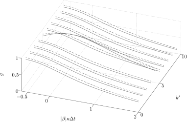
Refer to caption
Refer to caption
Figure 2: The normally-ordered correlation function for the Bose-Hubbard chain of 10 sites simulated using the truncated-Wigner approximation with response correction (solid line) and the TEBD-method (dashed line) for comparision. Left: the scaled modulus gNkk(t1,t2)subscript𝑔N𝑘superscript𝑘subscript𝑡1subscript𝑡2g_{\textrm{N}kk^{\prime}}(t_{1},t_{2}), right: the scaled phase ϕNkk(t1,t2)subscriptitalic-ϕN𝑘superscript𝑘subscript𝑡1subscript𝑡2\phi_{\textrm{N}kk^{\prime}}(t_{1},t_{2}), cf. Eqs. ( 111), (112), for k=5𝑘5k=5 and k=1,,10superscript𝑘110k^{\prime}=1,\cdots,10. The initial condition βk=2,k=1,,10formulae-sequencesubscript𝛽𝑘2𝑘110\beta_{k}=\sqrt{2},k=1,\cdots,10; J=0.1𝐽0.1J=0.1 and κ=1𝜅1\kappa=1. Graphs are plotted versus the scaled time |β|κΔt𝛽𝜅Δ𝑡|\beta|\kappa\Delta t with t2subscript𝑡2t_{2} chosen arbitrarily as t2=0.45subscript𝑡20.45t_{2}=0.45.

As we wish to have a “reference point” against which to compare our results, we can use either exact diagonalization, which forces us to limit the number of sites in the Bose-Hubbard chain to two or three or to use the time-evolving block decimation algorithm (TEBD) TEBD . The latter assumes small entanglement in the chain which is justified for not too large times and sufficiently small systems. In Fig. 2 we plot the result of the truncated-Wigner calculation of the normally-ordered correlation function for Ns=10subscript𝑁𝑠10N_{s}=10 sites and compare this to TEBD simulations. As the TEBD algorithm favors open boundary conditions we here (and only here) use these conditions. The figure shows the scaled modulus,

gNkk(t1,t2)=|GNkk(t1,t2)||β|2,subscript𝑔N𝑘superscript𝑘subscript𝑡1subscript𝑡2subscript𝐺N𝑘superscript𝑘subscript𝑡1subscript𝑡2superscript𝛽2\displaystyle{{\begin{aligned} g_{\textrm{N}kk^{\prime}}(t_{1},t_{2})=\frac{|G_{\textrm{N}kk^{\prime}}(t_{1},t_{2})|}{|\beta|^{2}},\end{aligned}}} (111)

(left), and the scaled phase,

ϕNkk(t1,t2)=argGNkk(t1,t2)|β|π,subscriptitalic-ϕN𝑘superscript𝑘subscript𝑡1subscript𝑡2argsubscript𝐺N𝑘superscript𝑘subscript𝑡1subscript𝑡2𝛽𝜋\displaystyle{{\begin{aligned} \phi_{\textrm{N}kk^{\prime}}(t_{1},t_{2})=\frac{\mathrm{arg}\,G_{\textrm{N}kk^{\prime}}(t_{1},t_{2})}{|\beta|\pi},\end{aligned}}} (112)

(right), of the correlation function for k=5𝑘5k=5 and ksuperscript𝑘k^{\prime} ranging from 1 to 10. In other words, each line in Fig. 2 corresponds to correlations between site 5 and either itself or some other site. All quantities are plotted versus the scaled time difference |β|κΔt𝛽𝜅Δ𝑡|\beta|\kappa\Delta t. The inital condition was chosen as the same coherent state |βkketsubscript𝛽𝑘|\beta_{k}\rangle in all modes with βk=2,k=1,,10formulae-sequencesubscript𝛽𝑘2𝑘110\beta_{k}=\sqrt{2},\ k=1,\cdots,10 (i.e., two quanta per mode). The hopping strength was set to J=0.1𝐽0.1J=0.1 and the interaction strength to κ=1𝜅1\kappa=1. The time t2subscript𝑡2t_{2} was chosen arbitrarily as t2=0.45subscript𝑡20.45t_{2}=0.45. The average for the truncated-Wigner method was over 80,0008000080,000 runs.

One recognizes a rather good agreement. Since the TEBD calculations are expensive we will resort in the following examples to the case of two and three modes, where direct numerical calculations in the full Hilbert space remain doable.
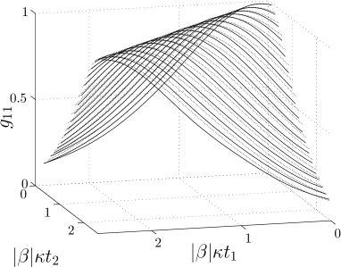
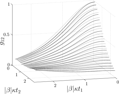
Refer to caption
Refer to caption
Refer to caption
Refer to caption
Figure 3: Comparison of the truncated-Wigner results (solid lines) to Hilbert-space ones (dashed lines) for the normally-ordered correlation function of the Bose-Hubbard chain of two sites. Top row: the scaled moduli g11(t1,t2)subscript𝑔11subscript𝑡1subscript𝑡2g_{11}(t_{1},t_{2}) (left) and g12(t1,t2)subscript𝑔12subscript𝑡1subscript𝑡2g_{12}(t_{1},t_{2}) (right), bottom row: the scaled phases ϕ11(t1,t2)subscriptitalic-ϕ11subscript𝑡1subscript𝑡2\phi_{11}(t_{1},t_{2}) (left) and ϕ12(t1,t2)subscriptitalic-ϕ12subscript𝑡1subscript𝑡2\phi_{12}(t_{1},t_{2}) (right). The initial condition is β1=β2=2subscript𝛽1subscript𝛽22\beta_{1}=\beta_{2}=\sqrt{2}; J=0.1𝐽0.1J=0.1 and κ=1𝜅1\kappa=1. The time t1subscript𝑡1t_{1} changes continuously while t2subscript𝑡2t_{2} is limited to discrete values ranging from 0.1 to 1.8.

In Fig. 3 we compare the results of the phase-space simulations (solid lines) to those in the Hilbert space (dashed lines) for the two mode case. The plotted quantities are g11(t1,t2)subscript𝑔11subscript𝑡1subscript𝑡2g_{11}(t_{1},t_{2}) (top left), g12(t1,t2)subscript𝑔12subscript𝑡1subscript𝑡2g_{12}(t_{1},t_{2}) (top right), ϕ11(t1,t2)subscriptitalic-ϕ11subscript𝑡1subscript𝑡2\phi_{11}(t_{1},t_{2}) (bottom left), and ϕ12(t1,t2)subscriptitalic-ϕ12subscript𝑡1subscript𝑡2\phi_{12}(t_{1},t_{2}) (bottom right). That is, the top row shows the modulus while the bottom row—the phase of the normally-ordered correlator; the left column depicts the same-site, while the right column—the neighbour-to-neighbour correlations. Dependence of all quantities on t1subscript𝑡1t_{1} and t2subscript𝑡2t_{2} is expressed naturally by 3D plots. However, while t1subscript𝑡1t_{1} changes continuously, t2subscript𝑡2t_{2} is limited to discrete values, t2=0.1, 0.2,, 1.8subscript𝑡20.10.21.8t_{2}=0.1,\,0.2,\,\ldots,\,1.8. The initial condition is a coherent state |βket𝛽|\beta\rangle with β=2𝛽2\beta=\sqrt{2} in each mode, the hopping strength is set to J=0.1𝐽0.1J=0.1 and the interaction strength to κ=1𝜅1\kappa=1. The average is over 80,000 runs. We see that the conditions imposed by number conservation, g11(t,t)=1subscript𝑔11𝑡𝑡1g_{11}(t,t)=1, ϕ11(t,t)=0subscriptitalic-ϕ11𝑡𝑡0\phi_{11}(t,t)=0, are clearly met in Fig. 3. Furthermore, the agreement between Hilbert space and the truncated-Wigner approximation is very good. The modulus of the correlation functions is always well reproduced. The phase appears to be not as well reproduced, but this impression is deceptive. In fact, error in phase increases when the modulus becomes small. Even in this case, the truncated-Wigner approach gives a reasonably good approximation to the phase of the correlation functions.
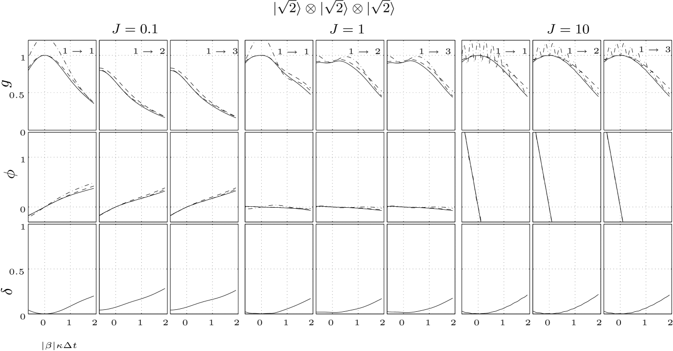
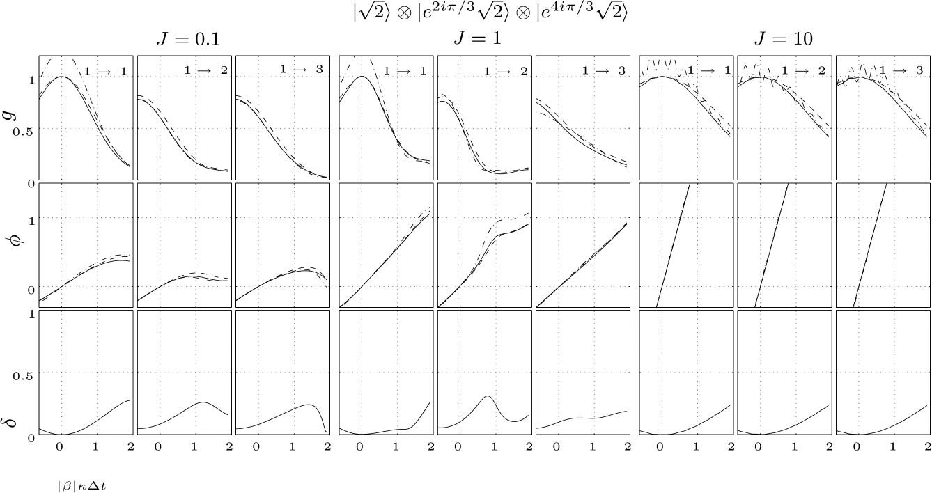
Refer to caption
Figure 4: The normally-ordered correlation function for the three mode Bose-Hubbard chain for the initial condition (113), κ=1𝜅1\kappa=1 and J=0.1,1,10𝐽0.1110J=0.1,1,10. Top row: the quantities g11(t1,t2)subscript𝑔11subscript𝑡1subscript𝑡2g_{11}(t_{1},t_{2}), g12(t1,t2)subscript𝑔12subscript𝑡1subscript𝑡2g_{12}(t_{1},t_{2}) and g13(t1,t2)subscript𝑔13subscript𝑡1subscript𝑡2g_{13}(t_{1},t_{2}); grouping of graphs with respect to the values of J𝐽J is self-explanatory. Truncated-Wigner calculations (solid lines), Hilbert-space results (dashed lines), and the uncorrected (symmetric) correlation function (dash-dotted lines). Middle row: the corresponding scaled phases ϕ11(t1,t2)subscriptitalic-ϕ11subscript𝑡1subscript𝑡2\phi_{11}(t_{1},t_{2}), ϕ12(t1,t2)subscriptitalic-ϕ12subscript𝑡1subscript𝑡2\phi_{12}(t_{1},t_{2}) and ϕ13(t1,t2)subscriptitalic-ϕ13subscript𝑡1subscript𝑡2\phi_{13}(t_{1},t_{2}). Bottom row: the relative error of the truncated-Wigner simulation compared to the Hilbert-space result. All quantities are plotted versus the scaled time difference |β|κΔt𝛽𝜅Δ𝑡|\beta|\kappa\Delta t with t2subscript𝑡2t_{2} choosen arbitrarily as t2=0.45subscript𝑡20.45t_{2}=0.45.
Refer to caption
Figure 5: The same as in Fig. 4 but for the initial condition (114).

A detailed comparison between the truncated-Wigner and Hilbert-space calculations for three sites may be seen in Figs. 4 and 5. The initial condition in Fig. 4 was chosen as three identical coherent states,

|𝜷=|β|β|β,(Fig. 4)ket𝜷tensor-productket𝛽ket𝛽ket𝛽(Fig. 4)\displaystyle{{\begin{aligned} \big{|}{\mbox{\rm\boldmath$\beta$}}\big{\rangle}=\big{|}\beta\big{\rangle}\otimes\big{|}\beta\big{\rangle}\otimes\big{|}\beta\big{\rangle},\ \ \ \textrm{(Fig.\ \ref{fig:GleicheBeta})}\end{aligned}}} (113)

with β=2𝛽2\beta=\sqrt{2}, while in Fig. 5 the coherent states differ in phases,

|𝜷=|β|βe2iπ/3|βe4iπ/3,(Fig. 5)ket𝜷tensor-productket𝛽ket𝛽superscript𝑒2𝑖𝜋3ket𝛽superscript𝑒4𝑖𝜋3(Fig. 5)\displaystyle{{\begin{aligned} \big{|}{\mbox{\rm\boldmath$\beta$}}\big{\rangle}=\big{|}\beta\big{\rangle}\otimes\big{|}\beta e^{2i\pi/3}\big{\rangle}\otimes\big{|}\beta e^{4i\pi/3}\big{\rangle},\ \ \ \textrm{(Fig.\ \ref{fig:VerschiedeneBeta})}\end{aligned}}} (114)

with the same β𝛽\beta. Calculations were performed for κ=1𝜅1\kappa=1 and J=0.1,1,10𝐽0.1110J=0.1,1,10. In both figures, the top row of graphs shows the quantities g11(t1,t2)subscript𝑔11subscript𝑡1subscript𝑡2g_{11}(t_{1},t_{2}), g12(t1,t2)subscript𝑔12subscript𝑡1subscript𝑡2g_{12}(t_{1},t_{2}) and g13(t1,t2)subscript𝑔13subscript𝑡1subscript𝑡2g_{13}(t_{1},t_{2}) plotted versus the scaled time difference |β|κ(t1t2)𝛽𝜅subscript𝑡1subscript𝑡2|\beta|\kappa(t_{1}-t_{2}), with t2subscript𝑡2t_{2} chosen arbitrarily as t2=0.45subscript𝑡20.45t_{2}=0.45. The grouping of graphs in Figs. 4 and 5 with respect to the values of J𝐽J is self-explanatory. The results of truncated-Wigner calculations using Eq. ( 106) are shown as solid lines, the dashed lines represent the Hilbert-space results, and the dash-dotted lines—the uncorrected (symmetrically-ordered) correlation function. The middle row of graphs depicts the corresponding scaled phases ϕ11(t1,t2)subscriptitalic-ϕ11subscript𝑡1subscript𝑡2\phi_{11}(t_{1},t_{2}), ϕ12(t1,t2)subscriptitalic-ϕ12subscript𝑡1subscript𝑡2\phi_{12}(t_{1},t_{2}) and ϕ13(t1,t2)subscriptitalic-ϕ13subscript𝑡1subscript𝑡2\phi_{13}(t_{1},t_{2}). The bottom row represents the relative error of the truncated-Wigner simulation compared to the Hilbert-space result,

δkk(t1,t2)=|GNkk(t1,t2)GHkk(t1,t2)1|.subscript𝛿𝑘superscript𝑘subscript𝑡1subscript𝑡2subscript𝐺N𝑘superscript𝑘subscript𝑡1subscript𝑡2subscript𝐺H𝑘superscript𝑘subscript𝑡1subscript𝑡21\displaystyle\delta_{kk^{\prime}}(t_{1},t_{2})=\bigg{|}\frac{G_{\textrm{N}kk^{\prime}}(t_{1},t_{2})}{G_{\textrm{H}kk^{\prime}}(t_{1},t_{2})}-1\bigg{|}. (115)

Phase space averages were taken over 80,0008000080,000 runs.

Once again, we see that the requirements imposed by number conservation are met in all results. For t1=t2subscript𝑡1subscript𝑡2t_{1}=t_{2}, g11(t1,t2)=1subscript𝑔11subscript𝑡1subscript𝑡21g_{11}(t_{1},t_{2})=1 and ϕ11(t1,t2)=0subscriptitalic-ϕ11subscript𝑡1subscript𝑡20\phi_{11}(t_{1},t_{2})=0.

The importance and accuracy of the response correction manifests itself pretty impressively for J=10𝐽10J=10 where the uncorrected phase-space solutions oscillate. This is not a numerical artifact because oscillations occur irrespective of the time step of the numerical integration. These oscillations cancel out with similar ocillations in the response term leaving the correlation function smooth and in good agreement with the Hilbert-space result.

Looking at the error plots one can recognize that the method performs well over the collapse time scale. It is worthy of stressing that we look at the relative and not at the absolute error. The error tends to get large for Δt1/|β|κΔ𝑡1𝛽𝜅\Delta t\rightarrow 1/|\beta|\kappa but actually this is only due to the fact that the absolute value of the correlation function is already very small.
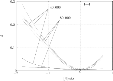
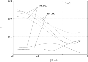
Refer to captionRefer to caption
Figure 6: Assessment of statistical errors for two mode case with J=0.1𝐽0.1J=0.1, κ=1𝜅1\kappa=1, |β=2(1,1)ket𝛽211|\beta\rangle=\sqrt{2}(1,1). Solid lines show the discrepancy between results derived from two independent runs with the same number of “coin tosses” (40,000 and 80,000). Dashed lines show the relative error of the same results compared to the exact (Hilbert-space) results. All graphs are plotted versus the scaled time |β|κΔt𝛽𝜅Δ𝑡|\beta|\kappa\Delta t, with t2subscript𝑡2t_{2} set arbitrarily to t2=1.3subscript𝑡21.3t_{2}=1.3. We see that the statistical errors are insignificant.

To develop a feeling for the statistical error, in Fig. 6 we compare the discrepancy between results obtained from two independent phase-space simulations with the relative error of the same pair of results compared to the exact (Hilbert-space) result, for the two mode Bose-Hubbard chain. The initial condition is a coherent state with β=2𝛽2\beta=\sqrt{2} in each mode. The hopping strength is set to J=0.1𝐽0.1J=0.1, and the interaction strength to κ=1𝜅1\kappa=1. The relative error between two correlation functions simulated in phase-space with the same number of “coin tosses” is shown as solid lines. The dashed lines are used for errors of the same pair of simulations in phase-space compared to the Hilbert-space solutions. The picture on top shows the said errors for the on-site average with k=k=1𝑘superscript𝑘1k=k^{\prime}=1, the one at the bottom for the averages between two modes, k=1𝑘1k=1, k=2superscript𝑘2k^{\prime}=2. All graphs are plotted versus the scaled time with t2subscript𝑡2t_{2} arbitrarily chosen as t2=1.3subscript𝑡21.3t_{2}=1.3.

It is evident from the figure that the statistical errors are insignificant. The discrepancy between results in phase-space are either just small, or small compared to the accuracy of the method. At times |β|κΔt𝛽𝜅Δ𝑡|\beta|\kappa\Delta t where the relative errors of the phase-space result compared to the Hilbert-space solution are of the same order as the errors of two independent runs in phase-space, the correlation function is already very small.

All in all, the “response correction” brings the results of the truncated-Wigner simulation in phase-space into a good agreement with the Hilbert-space simulations. Our observation for a single mode, that is, that the method gives good results over collapse time scales but fails on revival times, also holds for two and three modes. It is worthy of reminding the reader that all errors are solely due to the approximate nature of the truncated Wigner simulation. By itself, Eq. ( 106) is exact.

VI Summary

A phase-space path-integral approach generalising the symmetric representation of Schrödinger operators to the Heisenberg picture is developed, and “generalised phase-space correspondences” allowing one to commute Heisenberg operators with unequal time arguments are derived. The conventional truncated Wigner representation emerges as an approximation within the path-integral approach. This results in formal techniques allowing one to calculate time-normal averages of Heisenberg operators approximately with relative ease. These techniques have been verified for the Kerr oscillator and for the Bose-Hubbard model showing a good agreement with exact Hilbert space calculations at collapse time scales for surprisingly low numbers of oscillator quanta.

VII Acknowledgements

M.O. thanks the Institut für Quantenphysik at the Universität Ulm for generous hospitality. L.P. is grateful to ARC Centre of Excellence for Quantum-Atom Optics at the University of Queensland for hospitality and for meeting the cost of his visit to Brisbane. The authors are indebted to D. Muth, Univ. of Kaiserslautern, for the TEBD simulations. This work was supported by the Program Atomoptik of the Landesstiftung Baden-Württemberg and SFB/TR 21 “Control of Quantum Correlations in Tailored Matter” funded by the Deutsche Forschungsgemeinschaft (DFG), a scholarship “Mathematical Analysis of Evolution, Information and Complexity” at Ulm University, Australian Research Council, and a University of Queensland New Staff Grant. A.P. acknowledges support from AFOSR YIP and Sloan Foundation.

References

  • (1) L. Fallani, L. De Sarlo, J.E. Lye, M. Modugno, R. Saers, C. Fort, and M. Inguscio, Phys. Rev. Lett. 93, 140406 (2004).
  • (2) C.D. Fertig, K.M. O’Hara, J.H. Huckans, S.L. Rolston, W.D. Phillips, and J.V. Porto, Phys. Rev. Lett. 94, 120403 (2005).
  • (3) J. Mun, P. Medley, G. K. Campbell, L. G. Marcassa, D. E. Pritchard, and W. Ketterle, Phys. Rev. Lett. 99, 150604 (2007).
  • (4) Th. Anker, M. Albiez, R. Gati, S. Hunsmann, B. Eiermann, A. Trombettoni, and M.K. Oberthaler, Phys. Rev. Lett. 94, 020403 (2005).
  • (5) M. Albiez, R. Gati, J. Fölling, S. Hunsmann, M. Cristiani, and M.K. Oberthaler, Phys. Rev. Lett. 94, 010402 (2005).
  • (6) J.S. Caux, P. Calabrese, and N.A. Slavnov, J. Stat. Mech. (2007) P01008; P. Calabrese and J.S- Caux, Phys. Rev. Lett. 98, 150403 (2007).
  • (7) R.J. Glauber, Phys. Rev. 131, 2766, (1963).
  • (8) E.C.G. Sudarshan, Phys. Rev. Lett. 10, 277, (1963).
  • (9) P.D. Drummond and C.W. Gardiner, J. Phys. A 13, 2353, (1980).
  • (10) C.W. Gardiner, Quantum Noise, (Springer-Verlag, Berlin, 1991).
  • (11) P. Deuar and P.D. Drummond, Phys. Rev. Lett. 98, 120402 (2007).
  • (12) P.D. Drummond and J.F. Corney, Phys. Rev. A60, R2661 (1999).
  • (13) J.J. Hope and M.K. Olsen, Phys. Rev. Lett. 86, 3220 (2001).
  • (14) M.J. Steel et al., Phys. Rev. A58, 4824, (1998).
  • (15) L.I. Plimak, M.K. Olsen, and M.J. Collett, Phys. Rev. A64, 025801, (2001).
  • (16) P. Deuar and P.D. Drummond, Comp. Phys. Commun. 142, 442, (2001).
  • (17) P. Deuar and P.D. Drummond, Phys. Rev. A66, 033812, (2002).
  • (18) S.R. White and A.E. Feiguin, Phys. Rev. Lett. 93, 076401 (2004).
  • (19) G. Vidal, Phys. Rev. Lett. 93, 040502 (2004).
  • (20) M.J. Werner and P.D. Drummond, J. Comput. Phys. 132, 312, (1997).
  • (21) A. Sinatra, C. Lobo, and Y. Castin, Phys. Rev. Lett. 87, 210404, (2001).
  • (22) A. Sinatra, C. Lobo, and Y. Castin, J. Phys. B 35, 3599, (2002).
  • (23) M.K. Olsen, A.S. Bradley, and S.B. Cavalcanti, Phys. Rev. A70, 033611, (2004).
  • (24) A. Polkovnikov, Phys. Rev. A68, 053604 (2003).
  • (25) A. Polkovnikov and D.-W. Wang, Phys. Rev. Lett. 93, 070401 (2004).
  • (26) J. Ruostekoski, L. Isella, Phys. Rev. Lett. 95, 110403 (2005).
  • (27) R. Bistritzer and E. Altman, PNAS 104, 9955 (2007)
  • (28) R.G. Scott, D. A. W. Hutchinson, T. E. Judd, T. M. Fromhold, arXiv:0901.4602.
  • (29) S. Hofferberth, I. Lesanovsky, B. Fischer, T. Schumm, J. Schmiedmayer, Nature 449, 324 (2007).
  • (30) A. Polkovnikov, S. Sachdev, S. M. Girvin, Phys. Rev. A 66, 053607 (2002).
  • (31) A. K. Tuchman, C. Orzel, A. Polkovnikov, and M. Kasevich, Phys. Rev. A 74, 051601 (2006).
  • (32) P. B. Blakie, A. S. Bradley, M. J. Davis, R. J. Ballagh, and C. W. Gardiner, Advances in Physics 57, 363 (2008).
  • (33) P. Kinsler and P.D. Drummond, Phys. Rev. A44, 7848, (1991).
  • (34) M.K. Olsen, K. Dechoum, and L.I. Plimak, Opt. Commun. 190, 261, (2001).
  • (35) L.I. Plimak, M.K. Olsen, M. Fleischhauer, and M.J. Collett, Europhys. Lett. 56, 372, (2001).
  • (36) L.I. Plimak, M. Fleischhauer, M.K. Olsen and M.J. Collett, preprint cond-mat/0102483.
  • (37) M.K. Olsen, L.I. Plimak, S. Rebić, and A.S. Bradley, Opt. Commun. 254, 271, (2005).
  • (38) R. Kubo, Lectures in Theoretical Physics, v. 1 (Wiley, New York, 1959).
  • (39) R. Kubo, Rep. Prog. Phys. 29, 255 (1966).
  • (40) L.I. Plimak, Phys. Rev. A50, 2120, (1994).
  • (41) L.I. Plimak, M. Fleischhauer, M.K. Olsen, and M.J. Collett, Phys. Rev. A67, 013812 (2003).
  • (42) L.I. Plimak and S. Stenholm, Annals of Physics, 323, 1963 (2008), ibid. 323, 1989 (2008).
  • (43) L.I. Plimak et al., unpublished.
  • (44) M.K. Olsen, L.I. Plimak, M.J. Collett, and D.F. Walls, Phys. Rev. A62, 023802, (2000).
  • (45) A. Polkovnikov, Phys. Rev. A 68, 033609 (2003).
  • (46) A. Polkovnikov and V. Gritsev, Nature Physics 4, 477 (2008).
  • (47) Leonard Mandel and Emil Wolf, Optical coherence and quantum optics (Cambridge University Press, 1995).
  • (48) D.F. Walls and G.J. Milburn, Quantum Optics, Springer-Verlag, Berlin (1994).
  • (49) C. W. Gardiner and P. Zoller, Quantum Noise, third edition (Springer-Verlag, Berlin Heidelberg, 2004).
  • (50) G.S. Agarwal and E. Wolf, Phys. Rev. D 2, 2161 (1970)
  • (51) J.S. Schwinger, J. Math. Phys. 2, 407 (1961).
  • (52) A. Polkovnikov, unpublished.
  • (53) M. Greiner, O. Mandel, T. W. Hänsch, and I. Bloch, Nature, 419, 51 (2002).
  • (54) A.A. Norrie, R.J. Ballagh, C.W. Gardiner, and A.S. Bradley, Phys. Rev. A73, 043618, (2006).
  • (55) I. Bloch, J. Dalibard, and W. Zwerger, Rev. Mod. Phys. 80, 885 (2008) .
  • (56) Square brackets as a notation for the symmetric operator mapping (34) are always signalled by a phase-space argument immediately following the brackets. In the absence of such argument square brackets have their usual mathematical meaning.