Wavelet entropy filter and cross-correlation of gravitational wave data

Abstract

We present a method for enhancing the cross-correlation of gravitational wave signals eventually present in data streams containing otherwise uncorrelated noise. Such method makes use of the wavelet decomposition to cast the cross-correlation time series in time-frequency space. Then an entropy criterion is applied to identify the best time frequency resolution, i.e. the resolution allowing to concentrate the signal in the smallest number of wavelet coefficients. By keeping only the coefficients above a certain threshold, it is possible to reconstruct a cross-correlation time series where the effect of common signal is stronger. We tested our method against signals injected over two data streams of uncorrelated white noise.

I Introduction

Gravitational waves (GW) are expected to be emitted by a variety of cosmological and astrophysical sources and several detectors are now operating to directly observe such a signal.

Some sources has been thoroughly studied and the expected GW-signal they emit is well modeled, like binary coalescences (without spin) and spinning neutron stars. For this class of sources the standard, matched-filtering techniques can be adopted, which are able to dig well under the noise floor. However some astrophysical systems may emit signals which are poorly modeled at the moment, not to mention unknown sources. This is the case for spinning coalescing systems, stellar core collapse events, cosmological stochastic signal, to mention just a few, known cases.

In ordered to be able to spot these unmodeled signals it is necessary to use a wide net, capable of detecting any suspect excess noise in the data streams. Following this strategy several burst searches are performed by the LIGO/VIRGO ligovirgo as well as by the resonant antennas network Vinante:2006uk ; Astone:2008zz , in which the technique of cross-correlation of data streams between two (or more) detectors is employed, possibly jointly with other techniques, to identify GW-event candidate, see e.g.laura ; Abbott:2007wu ; Acernese:2007ek . The cross-correlation analysis consists in obtaining a suitable defined data stream out of two detector data streams, and check for anomalous excesses in it. Cross-correlation can also be used in combination with matched filtering technique.

Here we present a method to enhance to capability of cross-correlating techniques to detect GW-signals. Our method is based on a wavelet decomposition of the cross-correlation data stream. Wavelet decomposition have been already adopted in GW-data analysis, see e.g. Moh ; Syl . In particular the WaveBurst algorithm Klim ; Klim2 has been employed in the the LIGO/VIRGO burst search.

Wavelet decomposition is a time-frequency decomposition. Unlike in the familiar case of Fourier Transform, in wavelet decomposition the time and frequency resolution is a free parameter (though the time and frequency resolutions are not independent on each other). The method described in the following section is able to adaptively select the decomposition level, or time-frequency resolution, which is best for the generic data stream analyzed. In particular this method, presented in a different context in Sturani:2007tc , picks the resolution which gathers the power of the data stream in the smallest possible number of wavelet coefficients, enhancing the possibility of singling out excesses of cross-correlation. The resolution choice is obtained by considering an entropy function Wic , which is maximum when the power of the signal is equally distributed among all the coefficients and minimum when all the power is concentrated in only one coefficient. Once the best resolution has been individuated, by a process of thresholding the detection of correlation excesses can be enhanced with respect to the analysis obtained by simply cross-correlating the data streams without further processing.

The paper is organized as follows: in sec. II we describe the method, in sec. III we report the results obtained by analyzing a stream of white data sampled at 5kHz containing injections of short-duration signals. Sec. IV contains the conclusion of our analysis.

II The method: wavelet packet and entropy filter

A wavelet transform is used to transform a time series into a mixed time-frequency one. Given an initial series made of $N$ data points, with sampling $\Delta t_{0}$, it contains information on frequencies ranging from zero up to the Nyquist frequency $f_{max}=(2\Delta t_{0})^{-1}$. Different decomposition levels are available in a wavelet transform, labeled by a (limited) integer number $j$. At each level the wavelet-transformed data stream contains $N$ coefficients as the initial time series, arranged in $2^{j}$ layers, each with $N\times 2^{-j}$ coefficients. At level $j$ the time resolution is $\Delta t_{j}=2^{j}\Delta t_{0}$ and the frequency resolution is $\Delta f_{j}=2^{-j}f_{max}=1/(2\Delta t_{j})$. The coefficients in the $i^{\rm th}$ layer ($0<i<2^{j}$) refer to the frequency bins characterized by $i2^{-j}\leq f/f_{max}<(i+1)2^{-j}$.

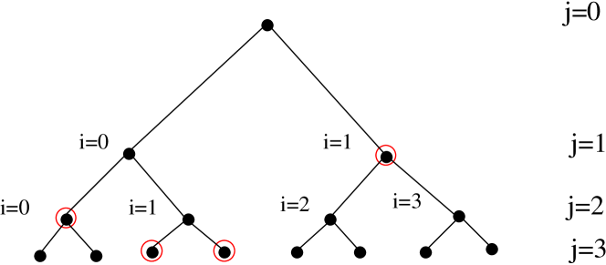
The output of a wavelet transform can be arranged in a binary tree where each node is an orthogonal vector subspace at level $j$ and at layer $i$. Together the layers of the same level contain exactly the same information of the original time series, so that complete reconstruction of the original signal is possible by collecting the coefficients of any level. Anyway this is not the only possible choice to reconstruct the original time-signal: it can be shown (see e.g. Mallat ) that other admissible trees $T$ completely represents the original signal in the wavelets domain, where an admissible tree is a sub-tree of the original binary decomposition tree where every node has exactly $0$ or $2$ children nodes, see e.g. fig. 1, where the nodes of an example of an admissible tree are marked by red circles. We denote an admissible tree by $T_{\{k,l\}}$, as it implies a choice of a set of pairs of level/layers.
Having such a redundancy, how to choose the set of subspaces to represent the signal? The standard choice is to take all the layers of a single decomposition level, but even in this case one has the freedom to pick among several levels.

The way we propose to choose in the set of admissible trees $T_{\{k,l\}}$ is based on an entropy function $E_{T}$ defined as follows:

$$E_{T_{\{k,l\}}}=-\sum_{i,j\in\{k,l\}}{x^{2}_{ij}\over{||X||_{T}^{2}}}\log{x^{2}_{ij}\over{||X||^{2}_{T}}}\,,$$ (1)

where the $x_{ij}$ are the wavelet coefficients of a level $j$ and layer $i$ and

$$||X||^{2}_{T}=\sum_{i,j\in\{k,l\}}{x_{ij}^{2}}\,.$$ (2)

From the complete decomposition tree, we select among all the possible admissible trees the one which have the minimum cost, i.e. the $\bar{T}$ for which $E_{\bar{T}}$ is minimum, following the entropy criterion (Wic where a different notation is used). From among all the admissible binary trees, $\bar{T}$ is the one that represents the signal most efficiently, as it uses the least possible number of wavelet coefficients.
For instance in the case in which only one of the $x_{ij}$’s is non-vanishing (maximal concentration) the entropy function is vanishing. On the other hand, if for some tree the decomposition coefficients are all equal, say $x_{ij}=1/N$, the entropy in this case is maximum, $\log N$.

Figure 1: Schematic example of a binary tree for a wavelet decomposition up to level 3. The layers in each level are explicitly labeled for $j<3$. The red circles show an example of a possible choice for a tree. In this examples it is made by choosing the subspaces with $\{j,i\}=\{(2,0),(3,2),(3,3),(1,1)\}$, from Sturani:2007tc .

After having performed the wavelet transform (a Symlet basis has been used) and the evaluation of the entropy function to determine the best tree, for each node in the resulting tree we set a threshold $\theta_{i,j}$ equal to a fraction of the value of the maximum wavelet coefficient $w_{i,j}$ in the node. Then a soft threshold function has been applied, i.e. each coefficient in the node has been changed according to the following function $f$:

$$f(w_{i,j}(k))=0$$ if

if

(3)

where $k$ ($0\leq k<N2^{-j}$) runs over the coefficients of the layer.

Then the time series has been recomposed from this mutilated wavelet coefficient set, where spurious disturbances (non concentrated in time and frequency) have been epurated. This will allow, as it is shown in the next section, to single out more clearly the excess in correlation due to actual signals. The wavelet decomposition has then been used to apply a non-linear filter to the r-series.

III Results

The cross correlation $r$ of two time series $\{x_{i}\},\{y_{i}\}$, each of length $N$, is given by

$$r=\frac{\sum_{i=1}^{N}(x_{i}-\bar{x})(y_{i}-\bar{y})}{\sqrt{\sum_{i=1}^{N}(x_{i}-\bar{x})^{2}}\sqrt{\sum_{i=1}^{N}(y_{i}-\bar{y})^{2}}}\,,$$ (4)

where an overbar stands for average value. Such quantity measures the correlation between two data streams, as it would be produced by a common GW signal embedded in uncorrelated detector noise laura and it compares waveforms without being sensitive to their relative amplitude. In real cases, data are usually filtered and/or whitened before applying the cross-correlation analysis. We have simulated two series of uncorrelated, white noise data. To test if our method is able to enhance the cross correlation output we have injected common signals of different amplitude and shape into the two data streams. For simplicity we have concentrated our attention on one kind of signal, an exponential-sine, whose time profile is given by:

$$h(t)=h_{0}\sin(2\pi f_{0}t)e^{-t/\tau}\qquad t>0\,,$$ (5)

(and $h(t)=0$ for $t<0$) for two different amplitudes, central frequency $f_{0}=920$Hz and $\tau={10,100}$msec. The amplitudes have been chosen so to reproduce an $SNR=0.47,0.71$,$2.24$ and $1.48$, where the SNR is defined as

$$SNR\equiv\sigma_{s}/\sigma_{n}\,,$$ (6)

where $\sigma_{n}$ is the noise standard deviation and $\sigma_{s}$ the signal standard deviations computed over a $5\tau$ period from the injection on. The correlation time-windows (determined by $N$ in eq. (4) and by the sampling time) are taken to be respectively $100$, $500$ msec for the $\tau=10,100$ msec injections.

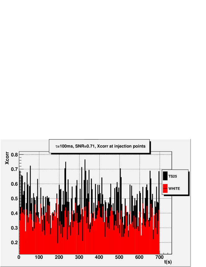
As an example, we report in fig. 2 the values of the maximum of the $r$-coefficients in correspondence of a series of injections (5).

Figure 2: Example of the cross-correlation of data streams for identical injections of the type (5) with $f_{0}=920$Hz,$\tau=100$ msec, correlation time-window of $500$ msec, $SNR=0.71$, as defined in eq. (6). The figure displays the maximum value of the $r$-coefficient for each injection (separated by 4 secs), before (red) and after (black) the wavelet entropy filter has been applied.

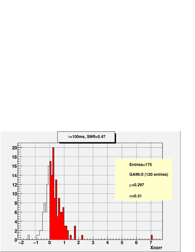
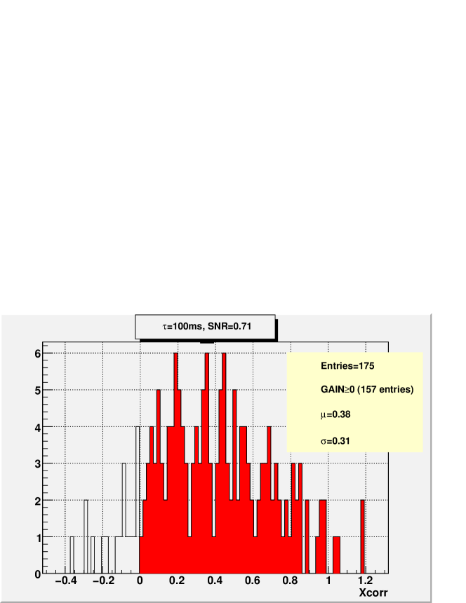
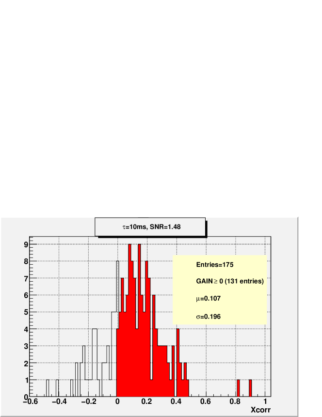
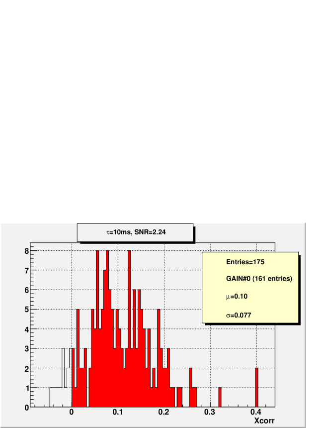
In order to quantify the enhancement due to the entropy filter we define a gain factor by considering, for each injection, the maximum value of the $r$-coefficient for the data before ($\bar{r}$) and after ($\bar{r}_{W}$) the treatment with the wavelet entropy filter and then define the quantity

$${\rm gain}=\frac{\bar{r}_{W}-\bar{r}}{\bar{r}}\,.$$ (7)

Figs. 4-6 show that for different choice of the injection parameters the wavelet entropy filter thus indeed lead to a statistical enhancement of the cross-correlation, the enhancement being stronger for stronger signals.

Figure 3: Histogram of gain factor, as defined by eq. (7) and correspondent average $\mu$ and standard deviation $\sigma$. Parameters $SNR$ and $\tau$ of the injections are displayed, $f_{0}=920$Hz.

Figure 4: Histogram of gain factor. Parameters $SNR$ and $\tau$ are displayed, $f_{0}=920$Hz.

Figure 5: Histogram of gain factor. Parameters $SNR$ and $\tau$ are displayed, $f_{0}=920$Hz.

Figure 6: Histogram of gain factor. Parameters $SNR$ and $\tau$ are displayed, $f_{0}=920$Hz.

In order to show that this method let excesses of correlation step out of the noise floor more clearly, while not introducing any significant increase of false alarm rate, we have evaluated the average and standard deviation of the maximum of the $r$-coefficients obtained by cross-correlating white data without any injection before and after the application of the entropy filter. The result summarized in tab. 2 shows that in absence of signal the application of the wavelet entropy filter is irrelevant.
On the other hand, analyzing the cross-correlation time series obtained by data with injections, and counting how many $\bar{r},\bar{r}_{W}$-coefficients have exceeded the average by more than 3$\sigma$ and 4$\sigma$ ($\mu$ and $\sigma$ reported in tab. 2), we have obtained the results reported in tab. 2, showing that the wavelet entropy filter is powerful in enhancing the detection of signals embedded into noise.

Correlation time-window	$\bar{r}$		$\bar{r}_{W}$
(msec)	$\mu$	$\sigma$	$\mu$	$\sigma$
$100$	0.21	0.14	0.21	0.15
$500$	0.041	0.081	0.040	0.075

Table 1: Background mean value $\mu$ and standard deviation $\sigma$ of the maximum cross-correlation coefficients obtained from white data (no injections) before ($\bar{r}$) and after ($\bar{r}_{W}$) the application of the entropy filter. The maximum is computed over a time-interval of $200$ msec.

		$\tau=10$ msec		$\tau=100$ msec
		SNR=2.24	SNR=1.48	SNR=0.71	SNR =0.48
$4\sigma$	#$\bar{r}_{W}$	127	14	153	38
	#$\bar{r}$	84	5	84	2
$3\sigma$	#$\bar{r}_{W}$	172	91	172	73
	#$\bar{r}$	169	70	151	28

Table 2: Number (out of 175 injections) of $\bar{r}$ and $\bar{r}_{W}$-coefficients at injection time exceeding by $3\sigma$ and $4\sigma$ the mean value of the $r$-coefficients of data without injections. The time-window for correlation are taken $100,500$ ms for $\tau=10,100$ ms respectively.

IV Conclusions

We have presented a method that makes use of a wavelet decomposition to determine which part of the cross-correlation time series can be zeroed without loosing interesting feature of the signals, thus reducing the impact of noise and we showed that this method can enhance the detection effciciency of signal embedded into noise while not increasing the false alarm rate. We plan to release the code to the gravitational wave community in a near future.

V References

References

- (1) F. Raab for the LSC, J. Phys.: Conf. Ser. 39 (2006) 25-31
- (2) A. Vinante [AURIGA Collaboration], Class. Quant. Grav. 23 (2006) S103.
- (3) P. Astone et al., Class. Quant. Grav. 25 (2008) 114048.
- (4) L. Cadonati, Class.Quant.Grav. 21 (2004), S1819-30.
- (5) B. Abbott et al. [LIGO Scientific Collaboration], Class. Quant. Grav. 24 (2007) 5343 [Erratum-ibid. 25 (2008) 039801] [arXiv:0704.0943 [gr-qc]].
- (6) F. Acernese et al. [AURIGA-EXPLORER-NAUTILUS-Virgo Collaboration], Class. Quant. Grav. 25 (2008) 205007 [arXiv:0710.3752 [gr-qc]].
- (7) S. Mallat, ”A wavelet tour in signal processing”, Academic Press, 1998.
- (8) Mohanty S, 2000 Phys. Rev. D 61 122002.
- (9) Sylvestre J, 2002 Phys. Rev. D 66 102004.
- (10) Klimenko S, Yakushin I, Rakhmanov M and Mitselmakher G 2004 Class.Quant.Grav. 21 S1685.
- (11) Klimenko S and Mitselmakher G 2004 Class.Quant.Grav. 21 S1819.
- (12) R. Sturani and R. Terenzi, J. Phys. Conf. Ser. 122 (2008) 012036 [arXiv:0711.0349 [gr-qc]].
- (13) Coifman, R. and Wickerhauser, M. V. (1992), ”Entropybased algorithms for best basis selection”, IEEE Transactions on Information Theory, 38, No. 2, 713-718.