The velocity distribution of nearby stars from Hipparcos data
I. The significance of the moving groups
Abstract
We present a three-dimensional reconstruction of the velocity distribution of nearby stars ( pc) using a maximum likelihood density estimation technique applied to the two-dimensional tangential velocities of stars. The underlying distribution is modeled as a mixture of Gaussian components. The algorithm reconstructs the error-deconvolved distribution function, even when the individual stars have unique error and missing-data properties. We apply this technique to the tangential velocity measurements from a kinematically unbiased sample of 11,865 main sequence stars observed by the Hipparcos satellite. We explore various methods for validating the complexity of the resulting velocity distribution function, including criteria based on Bayesian model selection and how accurately our reconstruction predicts the radial velocities of a sample of stars from the Geneva-Copenhagen survey (GCS). Using this very conservative external validation test based on the GCS, we find that there is little evidence for structure in the distribution function beyond the moving groups established prior to the Hipparcos mission. This is in sharp contrast with internal tests performed here and in previous analyses, which point consistently to maximal structure in the velocity distribution. We quantify the information content of the radial velocity measurements and find that the mean amount of new information gained from a radial velocity measurement of a single star is significant. This argues for complementary radial velocity surveys to upcoming astrometric surveys.
Section 1 Introduction
One of the key goals of Galactic astronomy—or near-field cosmology—is to understand the structure and evolutionary history of the Galaxy. Past and ongoing surveys have consistently found that the structure of the Galaxy is more complex than previously thought, and it is very likely, both from a theoretical perspective (Ghigna et al., 1998; Johnston, 1998; Helmi et al., 2003) as well as from an observational perspective (e.g., Koposov et al., 2008, 2009; Tollerud et al., 2008; Simon & Geha, 2007), that upcoming surveys will reveal much more complicated structures, and in much larger quantities, than those that are observed today. In the euphoria of a discovery, the statistical significance of the observed complexity is often only briefly touched upon. In order to make progress, however, it is important to ask the question whether the model, which can be arbitrarily complex, is warranted by the observations, or whether the structure in the data simply represents statistical fluctuations. This last point is not merely pedantic, as the significance and the reason for complex substructure has important ramifications for those who create models for the evolution and dynamical structure of the Galaxy and for those who interpret the observed substructure in a cosmological context. In the present set of papers we set out (i) to address this question of the complexity of the underlying distribution of an observed sample of stars using justifiable statistical methods in one specific example—the distribution of nearby stars in velocity space—and (ii) to assess the ramifications of the distribution that we recover and its complexity for questions concerning the structure and dynamics of the Galactic disk.
The discussion of the complexity of the structure of the Galaxy has traditionally focused on the number of components needed to give a good description of the observed distribution of stars in position, kinematics, metallicity, and age. And while the discussion has shifted mostly from a question at the beginning of the twentieth century about the appropriate number of “drifts” necessary to describe the kinematics of stars near the Sun (see below; Kapteyn, 1905; Schwarzschild, 1907) through a discussion about the number of distinct stellar populations (Baade, 1944, 1958; Roman, 1954; Oort, 1958; Schwarzschild, 1958) to an argument about the number of components that make up the large-scale structure of the Galaxy (in particular, the existence and properties of the “thick disk”; Gilmore & Reid, 1983; Bahcall & Soneira, 1980, 1984; Ivezić et al., 2008), this does not mean that the old controversies were ever fully resolved. Indeed, the history of the debate on the kinematics of stars in the local neighborhood provides a fine example of the analysis of the amount of structure, or lack thereof, in the phase-space distribution of stars and the consequences of the perceived structure for the fundamental parameters of the Galaxy.
1.1 The “transient” nature of moving groups
The first account of a common motion of stars appeared over 160 years ago in the Pleiades (Mädler, 1846). This common motion and the fact that the motions of stars further away from the center of the cluster seemed to be faster was then interpreted as indicating that the center of the Galaxy lies in the Pleiades, more specifically, that it coincides with Alcyone, the brightest star in the Pleiades cluster (Mädler, 1847). However, it was soon found that this was but a single instance of a more common phenomenon, as similar centers of common motion were also found to exist in other areas of the sky, i.e., in the Hyades cluster and for five of the bright stars in Ursa Major (Proctor, 1869).
The existence of the Hyades and the Ursa Major “moving groups”, as the groups of stars with a common motion are commonly called, was later confirmed and established on a firmer footing by the development of the convergent-point technique for the determination of the position of a cluster of stars (Boss, 1908; Hertzsprung, 1909). These groups, as well as the Pleiades moving group discovered earlier, have survived further scrutiny (Wilson, 1932; Roman, 1949; Dehnen, 1998) and we also unambiguously detect them in our data sample. After these successfull applications of this new technique it was widely used to find other moving groups and many were found in different areas of the sky—the Perseus moving cluster (Eddington, 1910), the 61 Cygni cluster (Boss, 1911; Russell, 1912), the Scorpio-Centaurus cluster (Plummer, 1913), the Vela moving cluster (Kapteyn, 1914), and the Corona Borealis moving cluster (Rasmuson, 1921). Most of these are now believed to be spurious (e.g. Rasmuson, 1921; Chaudhuri, 1940). The reasons for this failure of the convergent-point method to be a reliable indicator for the existence of moving groups were threefold: (1) it does not take into account the observational errors of the proper motions used and assumes that the space velocities of all of the individual stars in the cluster are exactly the same, which cannot hold in the presence of observational errors and which is not even close to true in the ideal case; (2) it assumes that all three of the components of the space velocity of the stars in the cluster are the same, but it is known that mixing in the direction out of the disk is much more efficient than mixing in the plane of the disk, such that groups of stars can share a similar motion in the components of the velocity in the plane of the disk much longer than they can do this in the direction out of the plane (and more precise determinations of the velocity distribution have shown that the distribution in directions out of the disk is essentially featureless, see Figure 20); (3) the tolerances with which a star has to meet the convergent-point test for cluster membership were gradually loosened, in order to deal with the complications described in the previous two points, leading to the inclusion of more and more spurious members. Thus, wrong conclusions were drawn about the amount of structure in the velocity distribution after the application of a technique that could not reliably determine the structure of the underlying distribution from an observed sample of stars, and that was stretched beyond where it was applicable in the best cases.
During the latter half of the twentieth century the business of claiming the existence of new moving groups—followed by calling their reality into question—remained in full swing. Eggen in particular was prolific in finding new moving groups and much of the discussion about their existence and members focused on their having a single stellar population, since all of the moving groups at the time were thought to be the remnants of disintegrating star clusters. About a dozen new moving groups were found by Eggen (Eggen, 1958; Eggen & Sandage, 1959; Eggen, 1959a, b, 1964, 1965, 1969, 1971a, 1971b, 1978) and different results for their chemical homogeneity and ages were found by different groups (e.g., Eggen, 1970; Williams, 1971; Boyle & McClure, 1975; Tuominen & Vilhu, 1979; Eggen, 1983; McDonald & Hearnshaw, 1983; Eggen, 1986; Proust & Foy, 1988). Most of these groups are not recovered in more recent analyses. The existence of the Hyades and Ursa Major groups was established on a firmer footing by ever growing samples of member stars (Ogorodnikov & Latyshev, 1968, 1970; Eggen, 1970; Boyle & McClure, 1975; Soderblom & Mayor, 1993), although their interpretation as dispersing star clusters was repeatedly called into question, especially in the case of the Hyades moving group (Wilson, 1966; Breger, 1968; Williams, 1971; Boyle & McClure, 1975; Soderblom & Clements, 1987; Boesgaard & Budge, 1988). Both of these groups were believed to contain significant fractions of the stars in the Solar neighborhood, but it was only after the advent of complete samples of stars with accurate astrometry with Hipparcos that this question could be studied in detail (with the exception of Grenier et al., 1985; Gomez et al., 1990).
1.2 The Hipparcos era
The astrometric ESA space mission Hipparcos, which collected data over a 3.2 year period around 1990, provided for the first time an all-sky catalogue of absolute parallaxes and proper motions with micro-arcsecond precision (ESA, 1997). Different complete samples of stars were extracted from the star catalogue, and many different methods were used to determine the distribution of these stars in velocity space and its overdensities (Chen et al., 1997; Figueras et al., 1997; Dehnen, 1998; Chereul et al., 1998, 1999; Asiain et al., 1999; Bienaymé, 1999; Skuljan et al., 1999). The picture that emerged from these various reconstructions of the velocity distribution was startling: the distribution was revealed to be extremely structured, with many, if not most, of the stars part of large associations of stars, in particular, the Hyades, Pleiades and Ursa Major moving groups (Dehnen, 1998). In addition to the confirmation of the moving groups, more complex structures such as several almost parallel branches and sharp edges in the distribution in the Galactic plane were also observed (Skuljan et al., 1999). Over the years, many radial velocities measurements have been made, most notably as part of the Geneva-Copenhagen Survey (Nordström et al., 2004), which has led to a confirmation of many of these structures (Famaey et al., 2005), and a proliferation of new moving groups has been found in the combination of the data sets (Antoja et al., 2008; Zhao et al., 2009). However, the existence of these new moving groups has not been convincingly shown to date.
The most popular method by far in recent years to determine the velocity distribution is the kernel density estimation technique (Silverman, 1986) and the related wavelet analysis technique for identifying moving groups (e.g., Slezak et al., 1990). This technique has been applied to the Hipparcos data at various degrees of sophistication. In the simplest form this method basically amounts to a smoothed histogram of the data in which each data point is replaced by a Gaussian probability distribution (the so-called “kernel”) with some fixed width around the observed value (Chen et al., 1997). When a kernel with a vanishing volume is chosen this technique is known as wavelet analysis, in which the kernel is a wavelet that picks out overdensities in the data (e.g., a “Mexican hat” wavelet, Murenzi, 1989). When applied with a fixed width this method naturally picks out the slightest overdensities of scale in the observed distribution. Therefore, it is unsurprising that setting km s-1 turns up a large number of overdensities of exactly this size (Francis & Anderson, 2009), which are then tentatively called new moving groups (Zhao et al., 2009), and finds substructure in the classical moving groups. Given the measurement uncertainties and the spatial extent of the Hipparcos sample—even a “cold” moving group on a circular orbit spread out over pc will create elongated structures in the velocity distribution with a size km s-1 2.5 km s-1—structure on these scales is unlikely to be real, unless they can be localized in position space as well. Slightly more sophisticated techniques set the smoothing scale in an optimal way given the kernel, the dimensionality of the distribution, and the number of data points (Cabrera-Caño & Alfaro, 1990; Asiain et al., 1999). This theoretically optimal value, however, generally leads to scales km s-1, such that the smoothing scale problem persists.
More sophisticated analyses realize that the measurement uncertainties limit the scales on which structure can be detected and that setting the scale parameter means setting the scale of the detected structure. Using more realistic values for the scale ( km s-1) and considering multiple scales returns merely the classical moving groups from a subset of the Hipparcos data (Figueras et al., 1997). Adaptive kernel methods are techniques in which the smoothing scale is allowed to vary from data point to data point, and a well-defined procedure for iteratively setting these different scales based on the reconstructed distribution and a leave-one-out cross validation procedure exists (Silverman, 1986). Using a sample of 4,000 Hipparcos stars the optimal overall smoothing scale was found to be km s-1 (Skuljan et al., 1999) and the reconstructed distribution showed only a few peaks.
Sophisticated multi-scale methods borrowed from astronomical image analysis have also been used a few times to determine the velocity field. These multiscale methods, such as the à trous method (Starck & Murtagh, 2006), smooth the observed density on different scales allowing the study of the velocity distribution on various scales (Chereul et al., 1998, 1999). These multiscale methods can be combined with denoising techniques, which filter the wavelet coefficients according to their significance assuming a prior distribution on the coefficients (e.g., Wiener filtering, Starck & Murtagh, 2006). Since the scales are still set by hand, if set to a small scale these methods still naturally find structures on the smallest scale analysed, leading to a large abundance of structure in the observed velocity distribution (Antoja et al., 2008).
The advantages of these kernel density and wavelet analysis techniques are that they are conceptually simple, non-parametric, and computationally inexpensive, as they behave for the most part as , where is the number of data points, multiplied by the number of scales for multiscale methods. One disadvantage of these techniques is that they only work in the case of complete data, i.e., data with all of the dimensions measured. Since Hipparcos did not measure the radial velocities of the survey stars, these techniques could not be applied to the Hipparcos catalogue by itself, instead they had to take small subsamples of the catalogue for which full phase space information was available or wait until the arrival of radial velocities for a selected number of stars. The main disadvantage, however, is that in the presence of sizeable measurement errors, as is the case in the determination of the velocity distribution from Hipparcos data for which the percent parallax uncertainties give rise to percent velocity errors, the kernel density estimate reconstructs the observed distribution and not the underlying distribution, i.e., they do not reconstruct the distribution you would find if you had “good” data, that is, data with vanishingly small uncertainties and all dimensions measured. The kernel density estimate and wavelet analysis techniques do not take into account the individual uncertainty properties of the data points, at best they let the overall uncertainty scale guide the choice of smoothing scale. In order to reconstruct the underlying velocity distribution it is necessary to convolve a model for the underlying distribution with the uncertainties of the individual stars and compare the resulting distribution with the observed distribution. When attempting to reconstruct the velocity distribution from incomplete data this is the approach that must be adopted.
Dehnen (1998) determined the velocity distribution from Hipparcos data alone. The underlying distribution was pixelized and the value in each pixel was obtained by a maximum penalized likelihood method. In order to compare the model with the data Dehnen used an uncertainty model that consisted of an infinite variance in the radial direction (the unobserved direction) and a zero variance in the tangential direction, as he believed that taking into account the individual errors in the tangential velocities was unnecessary given the sample size. This simplification leads to an unbounded likelihood function, which is why the function to be maximized had to include a penalty functional which penalizes rough distribution functions. Given the scarcity of the data and the large number of pixels necessary in three dimensions, Dehnen found that the Hipparcos sample only samples pixels in each direction for a three-dimensional reconstruction, and therefore he could only reliably reconstruct two-dimensional projections of the velocity field. This means that associating structures in different projections poses somewhat of a problem. The validation of the resulting velocity distribution consisted of comparing the reconstructed distribution for different subsamples of the data and the only reliably identifiable structures corresponded to the classical moving groups and a thick disk moving group, the Arcturus stream. Although Dehnen claimed that the various wiggles in the contours of the reconstructed velocity distribution correspond to real features, and some of these features are indeed present in later analyses, one has to remember that all of the samples derived from the Hipparcos catalogue overlap significantly and that therefore cross-validation between different analyses does not necessarily mean cross-validation between different samples. Dehnen’s was the first approach to utilize all of the relevant Hipparcos data in determining the velocity distribution and he showed that, through the use of a well-defined, justifiable algorithm designed to cope with missing data, the large number of Hipparcos measurements could give the best determination of the velocity field yet.
The first, and until now only, attempt to model the distribution of stars in a phenomenological way again confirmed the classical moving groups and found no evidence for new structure (Famaey et al., 2005). A mixture of different base groups was fitted by using a maximum likelihood method which correctly accounted for the observational uncertainties and the selection function (Luri et al., 1996). Each base groups consisted of a spatial distribution that was an exponential disk with a scale-height and was uniform in the Galactic plane, a velocity distribution that was Gaussian, a Gaussian luminosity distribution, and a correction for interstellar absorption. Six base groups were found to be necessary to provide an acceptable fit to the data by using a likelihood test, the Wilk’s test (Soubiran et al., 1990). This method, while being objective and well-justified, has some drawbacks. It assumes that groups in velocity space also share characteristics in other observables and it is highly parametric, since each clump in velocity space has very definite spatial and luminosity distributions associated with it. The model for the velocity distribution itself is also highly restrictive, as not only does it assume that each clump in velocity space has a Gaussian distribution, this Gaussian distribution is further constrained to be aligned with the Galactic plane (a vertex deviation is kept as a free parameter).
1.3 Now, why are we so special?
In this paper we use a technique which combines all of the good points of the techniques described above to reconstruct the velocity distribution. In Section 2 we describe our model of the underlying distribution function, which consists of a mixture of three-dimensional Gaussian distributions, which are left completely free. We keep the number of Gaussian components as a free parameter such that this technique is non-parametric in the sense that a mixture of a sufficiently large number of normal distributions can fit any distribution function desired and we let the data decide the complexity of the model instead of setting the number of components by hand. Since our confrontation of the model with the data includes convolving the model with the individual uncertainties of the observations, this technique correctly takes care of measurement uncertainties and consequently can deal with missing data. This allows us to use one large sample of stars, i.e., the sample of tangential velocities from Hipparcos used by Dehnen (1998), to determine the velocity distribution and a different, non-overlapping, sample of observations, i.e., radial velocity measurements of stars from the Geneva-Copenhagen Survey, to validate the reconstructed velocity distribution. Any structure in the velocity distribution that passes this truly hard test can then confidently be considered real. We will see that few do.
In addition to this, since we obtain a semi-parametric representation of the three-dimensional velocity distribution we are equipped to consider different subspaces of this distribution, such that we can make predictions for the velocities of individual stars, both only knowing their position as well as conditioning on any known components of the velocities, which allows us to answer questions as to how much information is contained in lower-dimensional projections of the velocity distribution. For instance, we can ask how much information about the velocity distribution is gained from a knowledge of the radial velocities in addition to the tangential velocities. Such a question is important to ask in the context of the Gaia mission, which will not measure radial velocities for a large part of its catalogue (Perryman et al., 2001).
Finally, with the model of the velocity distribution in hand we can determine the peaks in the distribution and compare them to the known moving groups. The algorithm used in the optimization naturally returns probabilities for individual stars to be members of moving groups which allows us to study the members of the groups and, thus, the properties of the moving groups themselves. This will be pursued further in paper II in this series.
Section 2 Data, model, and algorithm
Throughout we use the standard Galactic velocity coordinate system, with the directions , , and (and associated unit vectors , , and ) pointing toward the Galactic center, in the direction of circular orbital motion, and toward the north Galactic Pole, respectively. Vectors are everywhere taken to be column vectors. The components of the velocity vector, , , and , are conventially referred to as , , and , respectively, but we will refer to them as , , and .
2.1 Hipparcos measurements
In this study we use a kinematically unbiased sample of 11,865 nearby main-sequence stars (Dehnen & Binney, 1998) from the Hipparcos catalogue (ESA, 1997). This sample is the union of two kinematically unbiased subsamples of Hipparcos stars: One subsample consists of a magnitude-limited subsample (complete to about 7.3 to 9 mag depending on Galactic latitude) and the other subsample contains a sample of stars south of judged from their spectral classification to be within 80 pc from the Sun. Main-sequence stars with relative parallax errors smaller than 10 percent and not part of a binary system were selected from both of these subsamples. The relative parallax error cut, while biasing the sample towards brighter stars, which have smaller parallax errors, as well as towards closer stars, which have larger parallaxes, does not affect the fact that the sample is kinematically unbiased, since the precision of the parallaxes in Hipparcos is mainly limited by Poisson noise and the accuracy of the attitude reconstruction of the Hipparcos satellite, both of which are unrelated to the kinematics. For the stars in this sample we take the equatorial coordinates, parallaxes, and proper motions from the new reduction of the Hipparcos data (van Leeuwen, 2007a, b). Although follow-up radial velocity measurements for the Hipparcos stars were suggested (Gerbaldi et al., 1989), radial velocities of many of the stars in this sample are unavailable. Because of the known issues of including radial velocities of only a subsample of stars (e.g., Binney et al., 1997), we give each star a radial velocity of zero, with an uncertainty that is many orders of magnitude larger than any of the velocities involved in this problem. For the purposes of the deconvolution technique described below, this approach is equivalent to an incomplete data approach, since the model and objective function that we use properly treat the uncertainties associated with the data (we have explicitly checked this).
The properties of the selected sample of stars in the observed quantities are shown in Figure 1. One can clearly see the overdensities near the poles of the ecliptic in the vs. plots. These overdensities are a consequence of both the scanning strategy of Hipparcos, which covers stars near the ecliptic poles much better than those near the ecliptic plane, leading to higher accuracies of the Hipparcos parallaxes near the ecliptic poles (see also the parallax vs. plots), as well as, for the south ecliptic pole, the inclusion of the sample of stars restricted to . The structure vs. and vs. panels is simply due to the Solar motion with respect to the Local Standard of Rest.
The components of the three-dimensional velocities of the stars in terms of the observed (,,,,,) is given by
| (1) |
where , [] = km s-1, [] = as, []=[]= as yr-1, and the matrices and are given by
| (2) |
and
| (3) |
respectively. In the context of the deconvolution technique that we use below to fit the velocity distribution we will define the observations to be and the projection matrix to be . Since we do not use the radial velocities of the stars, we set to zero in . The matrix depends on the epoch that the data were taken at (1991.25 for Hipparcos) through the values of , , and (the position in celestial coordinates of the north Galactic pole, and the Galactic longitude of the north Celestial pole, respectively). These quantities were defined for the epoch 1950.0 as follows: (Blaauw et al., 1960): , , and . This transformation is the only processing of the data which we perform beyond the sample cut. This means that we make no corrections for the effects of Galactic rotation—the effect of which is of the order of the observational uncertainties anyway—and do not subtract out the velocity of the local standard of rest, since we simply want to study the distribution of stellar velocities with respect to the Sun.
The Hipparcos catalogue entries, which can be represented by some vector for each star, come with single-star uncertainty covariance matrices 111These covariance matrices can be constructed from the upper-triangular weight matrices included in the new reduction of the Hipparcos data as (4) . If we write the derivative of the observations with respect to the catalogue entries in terms of a matrix ,
| (5) |
then the measurement uncertainty covariances for the are given by
| (6) |
This is only accurate in the regime of small parallax errors in which we are working. Star–to–star covariances in the Hipparcos data could be significant, e.g., through uncertainties in the modeling of the sattelite altitude; they are believed to be insignificant and are not reported in the Hipparcos catalogue. Although significant star–to–star correlations existed in the original Hipparcos catalogue, these are reduced by a factor 30 to 40 in the new reduction (see Figure 2.11 in van Leeuwen, 2007a).
2.2 Model and objective function
The model for the velocity distribution and the objective function which we use here has been described before (Hogg et al., 2005) and is described in great detail in Bovy et al. (2009). Here we summarize the most important aspects of the model and the objective function. We refer the reader to Bovy et al. (2009) for a more detailed derivation of the following results.
The method for density estimation from noisy data used here is completely general, and we will describe it in general terms before specifying it to the problem at hand. Our goal is to fit a model for the distribution function of a -dimensional quantity using only a set of observational data points . In general, we assume that these observations are noisy projections of the true values
| (7) |
where the noise is drawn from a normal distribution with zero mean and known covariance matrix . As described above, in this specific application we use a formally infinite eigenvalue—in practice a value much larger than any of the measured values —in the covariance matrix for the missing radial velocity, in which case no actual projection occurs and the operator is simply a rotation matrix, whose inverse is given by the product as described in the previous subsection. Although our method permits arbitrary variances and covariances in the observed properties of any data point (star), it assumes that there are no point–point (star–star) covariances. This is only true approximately in most cases of interest.
We will model the distribution function of the true values as a mixture of Gaussians:
| (8) |
where the amplitudes sum to unity and the function is the -dimensional Gaussian distribution with mean and variance tensor . We emphasize here that the number of Gaussians is a free parameter describing qualitatively different models for the distribution function and that its value therefore needs to be set by a model comparison technique. We will have much more to say about this later.
The probability of the observed data given the model parameters is then given by a simple convolution of the model with the error distribution (or, in probabilistic language, by a marginalization over the true values of the velocities)
| (9) |
which works out to be itself a mixture of Gaussians
| (10) |
where
| (11) |
because of the convolution of the model Gaussians with the uncertainty Gaussians..
For a given value of , the free parameters of the density model can then be chosen such as to maximize (the logarithm of) the total probability of the data given the model, or equivalently, (the logarithm of) the likelihood of the model given the data
| (12) |
For each , optimization of this function gives the best fit density model consisting of Gaussians. This optimization could be performed by any generic optimizer, such as nonlinear conjugate gradients. It is complicated, however, by the constraints on the parameters of the model, e.g., the amplitudes have to add up to one, the covariances must be positive definite. For this reason we opt for an optimization technique known as expectation–maximization (EM; Dempster et al., 1977), which views both the true values of the velocities as well as the components from which they were drawn as hidden variables and optimizes the probability of the full data. Readers not interested in this technique can safely skip the next subsection.
2.3 EM optimization algorithm
We will only give a brief, self-contained description of the EM technique we used to optimize the likelihood of the model of the velocity distribution function given a set of noisy, heterogeneous, and incomplete observations. Part of this algorithm has been described before (see the appendix of Hogg et al., 2005) and a full description and proof of the method outlined in this section can be found in Bovy et al. (2009). We would also like to point out that this algorithm was developed independently before (Diebolt & Celeux, 1989, unpublished; Diebolt & Celeux, 1990, unpublished) and applied to the velocity distribution in the Solar neighborhood (Gomez et al., 1990; Figueras et al., 1997) for a small number of components and without any of the extensions described below.
The EM algorithm works by introducing the following sets of hidden variables: (1) for each observation a set of “indicator variables” , which indicate for each component of the mixture of Gaussians whether this velocity was drawn from it, (2) for each observation the true velocity . Because the velocities are not actually drawn from single components but rather from the full mixture, the indicator variables take values between zero and one and correspond to the probability that a velocity was drawn from a component . Given these hidden variables—equivalently, given full data—the likelihood of the model is given by
| (13) |
This likelihood function can be optimized analytically. The strategy of any EM algorithm is now to take, in the first step, the expectation of this full-data likelihood given the data and a previous guess of the model parameters (this stage is appropriately called the expectation step) and then to maximize this expectation value in the second step (the maximization step). Given an initial guess for the model parameters, these two steps are performed iteratively until convergence, identified here, as is usual, by extremely small incremental improvement in the logarithm of the likelihood per iteration.
In taking the expectation of we need the expectation of the quantities , , and given the data and a current guess for the model parameters. Using some standard results from multivariate normal theory it is easy to show that
| (14) | ||||
| (15) |
while the expectation of the indicator variables is simply given by the posterior probability that was drawn from component
| (16) |
Given the expectation of the full-data likelihood, it then follows that the following update steps maximize this expectation value
| (17) |
where . Using Jensen’s inequality one can show that these expectation and maximization steps also lead to a monotonic increase in the probability of the observed data given the model (given in equation [12]).
Some problems that are commonly encountered using the EM algorithm to iteratively compute maximum likelihood estimates of the parameters of a Gaussian mixture are singularities and local maxima. Singularities arise when a Gaussian component becomes very peaked or elongated. The standard method to deal with this problem is to introduce a prior distribution for the model covariances, e.g., a Wishart density (Ormoneit & Tresp, 1996). Since the Wishart density is a conjugate prior for the covariance of a multivariate normal distribution (e.g., Gelman et al., 2000), the update steps in equation (2.3) are modified only slightly (in the simplest case) by the introduction of a regularization parameter in the update step for the covariances
| (18) |
where, again, . This regularization parameter is another free parameter which is not known a priori, but should be inferred from the data (in the context of Bayesian inference it is known as a hyperparameter). We will discuss its determination in detail below.
The fact that the EM algorithm monotonically increases the likelihood of the model given the data is both one of the advantages as well as one of the disadvantages of the EM method. The algorithm is very stable because of this property, leading to reasonable answers largely irrespective of the initial guess for the model parameters. However, because the likelihood cannot but increase in every step, the algorithm can easily get stuck in a local maximum of the likelihood function. In order to deal with this problem, we have to discontinuously change the model parameters to jump to a different region of parameter space. One way of doing this is by merging two of the Gaussians in the mixture and splitting a third Gaussian, thus conserving the number of Gaussians, after an initial run of the EM algorithm, and reconverging (Ueda et al., 1998). The new solution is then accepted if the likelihood of the model is larger than it was before this split and merge step. This procedure is halted after a sufficiently large number of possible split and merge steps fail to give an improvement of the likelihood of the model. We again refer the reader to Bovy et al. (2009) for details on how the Gaussians are merged and split and how the ranking of split and merge candidates is established.
2.4 The Geneva-Copenhagen Survey
In what follows, we fit a model of the velocity distribution using only the tangential velocities measured by Hipparcos, and then later we validate our results using radial velocity measurements. The radial velocity measurements which we use for this purpose are all taken from the Geneva-Copenhagen Survey (GCS; Nordström et al., 2004). The GCS catalogue consists of metallicities, ages, and kinematics for a complete, magnitude-limited, and kinematically unbiased sample of 16,682 nearby F and G dwarfs. We select from this sample all of the stars that have a Hipparcos entry and exclude any star that is suspected to be a giant or part of a binary system; this leaves us with 7,682 stars. For these stars we only take the radial velocities and the uncertainty in the radial velocities from the GCS catalogue, using the new reduction of the Hipparcos data to provide all of the other kinematical information. We performed no processing of the data beyond the sample cut.
Section 3 Application to Hipparcos data
Two-dimensional projections of the reconstructed three-dimensional velocity distribution for models characterized by different values of the number of Gaussians and the regularization parameter , which, in a sense, sets the smallest scale on which we can infer structure in the velocity distribution, are shown in Figures 2-4, although in high density regions a large amount of data trumps the regularization as can be seen from equation (18). The regularization parameter is expected to be of order one because of the typical magnitude of the velocity errors and because of the spatial range of the sample of stars: a “cold” moving group on a circular orbit spread out over the range of our sample, pc, will create elongated structures in the velocity distribution with a size km s-1 2.5 km s-1; the typical uncertainties in the velocities are of the same size and thus blur these elongated structures.
For each (,) pair two runs of the optimization algorithm were made. One started from randomly chosen initial conditions for all of the components of the mixture, the other one started with the best result obtained for the less complex models—models with lower , models with larger , or both—and added a small-amplitude new Gaussian component when necessary (this is unnecessary when the best result for the less complex models occurs for a model with the same but larger ). After optimization we then choose the reconstructed velocity distribution with the highest likelihood.
The classical moving groups are present in each reconstruction of the velocity field for all but the smallest values of . Projections of the distribution involving the component of the velocity are, as expected, essentially featureless for all of the considered values of and . The similarity of all of the reconstructions shows that the gross features—the rough overall shape and the main peaks—of the velocity distribution are very robust to the model selection question: Each of the models with reproduces the most salient features of the velocity distribution.
The logarithm of the likelihood of the different models given the observed tangential velocities is shown in Figure 5. As complexity increases with increasing (more components) and decreasing (less restrictions on the covariances) the likelihood of the models increases in these directions of increasing complexity; in Figures 2-4 this increase in complexity translates into smaller and smaller substructures coming to the surface in the velocity distribution. The increasing complexity of the velocity distribution is not confined to the projection onto the Galactic plane of the velocity distribution, small-scale features can also be seen in the projections that involve the vertical direction. We could further increase the likelihood of our model of the velocity distribution by adding more and more complexity to our model. The more important issue here is how much complexity is warranted by the data. This is the question which we discuss in the next section.
Section 4 The complexity of the model
In order to determine which combination of the model parameters and gives the best description of the underlying velocity distribution we will perform a series of model selection tests. Most of these tests are internal tests, meaning that they only use the data that was used to fit the velocity distribution (in our case these are the tangential velocities from the Hipparcos data), but we will perform one external test: We will use the reconstructed velocity distributions for each set of and to predict the radial velocities of the stars in the GCS catalogue and test these predictions. The preferred model is then the model that best predicts the radial velocities. From the outset we can say that an external test like this is to be preferred since it gives the strongest, most independent test of the validity of the reconstructed model of the velocity distribution.
4.1 Internal model selection tests
One of the simplest, and most robust, internal tests that we can perform is leave-one-out cross validation (Stone, 1974). In the most ideal application of this technique one creates data samples by leaving out one data point (the measurements for one star here) at a time and performs the full maximum likelihood fit of the velocity distribution for each of these data samples. Then one records the logarithm of the probability of the data point that was left out given the model found by fitting to all of the other data points and one adds up all of the log probabilities found in this way. The model to be preferred is then the model that gives the highest total probability of the left out data points. Why will this work? This procedure punishes models that overfit the data, that is, complex models that use their complexity to fit very specific features consisting of a small number of stars.
While simple, this technique can be computationally very expensive, as the analysis, which can be hard for even one data set, has to be repeated for data sets of roughly the same size, for each value of the parameters and . In practice one therefore often chooses to leave out a certain fraction of the data sample at each stage, e.g., 1 percent of the data, and record in each step the total probability of the left out fraction of the data. However, for the current application this still turns out to be much too computationally expensive, and we therefore chose to only allow the amplitudes of the component Gaussians to change from their maximum-likelihood values from the global fit for each of the leave-one-out trials.
Akaike’s information criterion (AIC) is a model selection criterion rooted in the concept of entropy, considering the amount of information lost when representing the data by the model (Akaike, 1974). We use an interpretation of the AIC which was developed for model selection in the context Gaussian mixture modeling (Bozdogan, 1983; Windham & Cutler, 1992). The AIC is defined as
| (19) |
where is the maximum number of components one would consider (which we set to 100), is the number of parameters per component, is the total number of parameters estimated, and is the logarithm of the probability of the data given the best estimate of the velocity distribution given and .
Another set of model selection criteria make use of the principle of minimum message length. According to this principle the best model of the data is the model that allows for the shortest full description of the data. It can be thought of as implementing Occam’s razor in a more sophisticated way than the chi–squared per degree of freedom folklore. The message length corresponding to a given model consists of the sum of the length of the message required to communicate the model parameters and the length of the message that transmits the residuals of the data given the model. As such, the message length is equivalent to the Kolmogorov complexity, the length of the shortest program that could output the data, which is, in general, incomputable (Solomonoff, 1964a, b; Kolmogorov, 1965). Therefore, in order to create a working model selection criterion based on the principle of minimum message length certain restrictions to the set of allowed codes must be made (Wallace & Dowe, 1999).
One such set of restrictions that does not make any assumptions about the process that generated the data is offered by the minimum description length principle (Rissanen, 1978; Grünwald, 2007). The minimum description length is given by (Rissanen, 1978; Schwarz, 1978)
| (20) |
Another, in some sense, Bayesian approach to the minimum coding inference principle is given by minimum message length (MML; Wallace & Boulton, 1968; Wallace, 2004). In minimum message length one’s prior beliefs about the data generating process are used in full in the encoding process, such that the message is formed by taking the prior assumptions about the model together with the data to find the shortest description of the data and the model. Minimum message length goes through great pains to come up with the shortest message length, leading to the following expression for the message length for the case of Gaussian mixtures (Wallace & Freeman, 1987; Oliver & Baxter, 1994; Oliver et al., 1996)
| (21) |
In this the are the eigenvalues of for each component ; is the observed covariance matrix of the distribution. We determine this covariance matrix by fitting a single Gaussian distribution to the observed sample of stars in the same way as we fit multiple component mixtures to the velocity distribution. is the optimal lattice quantizing constant in an -dimensional space. The reason this optimal lattice quantizing constant appears in the MML expression is that in order to minimize the message length one has to find the accuracy to which the model parameters are specified which minimizes the message length, that is, one has to quantize the model parameter space in an optimal way. This involves setting the overall accuracy scale—by specifying the volume of a quantum—but also, for each scale, finding the optimal arrangement of quantized values of the model parameter space for that scale. This latter optimization amounts to minimizing the squared-error made when quantizing and the optimal lattice quantizing constant is the constant of proportionality between the minimum squared-error and the product of the scale raised to the appropriate power— when the scale is the quantum of volume in the model parameter space—and , the dimension of the space. For example, optimal quantization of a one-dimensional quantity is achieved by using intervals of constant width and the minimum squared-error is given by , the value of the squared error for a uniform distribution. Therefore, the optimal lattice quantizing constant in one dimension is equal to 1/12. The scale of quantization itself is set based on the precision to which the model parameters are known, which is approximated using the Fisher matrix in the expression above.
In more than one dimension the optimal arrangement of quantized values is not in general a simple cubic lattice—indeed, this optimal arrangement is unknown in more than three dimensions—and the value of the optimal lattice quantizing constants are not known in more than three dimensions either (Conway & Sloane, 1992), although tight bounds on the value of the optimal lattice quantizing constant exist (Zador, 1963, 1982)
| (22) |
as goes to infinity, . For our purposes the dimensionality at which we evaluate these lattice quantizing constants are very high and the results we find later do not depend on whether we choose the upper or the lower bound in equation (22). The expression for the shortest message length given in equation (21) is still only an approximate expression, assuming that the components of the mixture do not overlap significantly. This is obviously not the case in the application to the velocity distribution, as can be seen from Figures 2-4, but it is a necessary assumption in order to calculate the shortest message length.
Finally, we also use the actual Bayesian model selection criterion, known as the evidence. The evidence is defined as the denominator in the application of Bayes’s theorem to parameter estimation, which in this case given by
| (23) |
in which is the likelihood of the model. Choosing uninformative priors for the model parameters, the evidence can be approximated as
| (24) |
in the case of a Gaussian mixture (Roberts et al., 1998). The are defined in equation (16), and the other quantities appearing in this equation have the same meaning as in equation (21).
Next we will discuss an external test for the complexity of the reconstructed velocity distribution.
4.2 Validation with the GCS radial velocities
Given our three-dimensional reconstruction of the velocity distribution in the Solar neighborhood, based solely on the tangential velocities from Hipparcos, we can validate each model of the velocity distribution using an external data set. The external data set which we use here is a set of radial velocities from the Geneva-Copenhagen Survey, which was described above in Section 2.4. For each set of and we proceed as follows: for each star in the sample taken from the GCS we predict the distribution of the radial velocity from the reconstructed velocity distribution and we record the probability of the actual measured radial velocity given this predicted probability distribution for the radial velocity. The “best” model for the true velocity distribution is then given by that set of (, ) that leads to the overall highest probability of the measured radial velocities.
How do we predict the probability distribution of the radial velocity for a given star given our three-dimensional model for the velocity distribution? We can distinguish two distinct predictions: we can base our prediction on the position of the star on the sky, or we can base our prediction both on the position of the star as well as on the observed tangential velocity of the star. It is this last prediction which we will use in order to compare different models for the velocity distribution.
Given the position of a star on the sky we know the radial direction from which we can construct the projection onto the radial direction. We define the radial and tangential projection operators by
| (25) |
in which is the unit matrix. We can then decompose the velocity distribution as
| (26) |
Marginalizing over the value of the tangential velocity is then simply performed by dropping the tangential directions from these Gaussians, such that
| (27) |
In order to obtain the probability of an observed radial velocity given this prediction, we need to go one step further. Since the measured radial velocities come with their own uncertainties, we need to convolve this predicted distribution with the error distribution of the measured value. Assuming that this error distribution is a Gaussian with zero mean and variance , the predicted distribution becomes
| (28) |
Since we know the tangential velocities of the stars in the GCS, we can use this information to make a more informed prediction for that star’s radial velocity. In order to do this we start again from equation (26), but this time we condition this distribution on the value of the tangential velocity. For each of the Gaussian components in equation (26) this conditioning basically comes down to performing a linear regression along the principal axes of the Gaussian ellipsoids, evaluated at the value of the tangential velocity. This linear regression needs to be performed while taking into account the uncertainties in all of the quantities, i.e., the full error covariance matrix of the tangential velocities , and the uncertainty on the radial velocity (since the uncertainties in the radial velocities are uncorrelated with the Hipparcos uncertainties). Using some standard results from multivariate normal theory the predicted distribution of the radial velocity of a star given its position and tangential velocity follows:
| (29) |
in which is calculated as in equation (16),
| (30) | ||||
| (31) |
and is the tangential velocity.
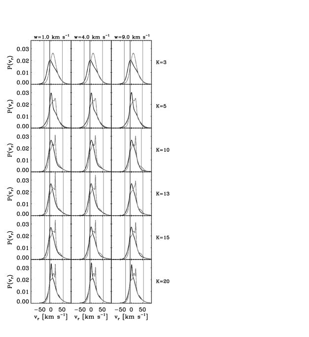
In Figure 6 the marginalized and conditioned predictions as well as the observed value are shown for a random sample of radial velocities from the GCS, for the particular values of and that we will adopt below as our fiducial values. The marginalized predictions are simply slices through the velocity distribution in the radial direction for that star, and therefore they are all rather broad. The conditioned distribution in many cases shifts much of the mass of the probability distribution to one or two sharp peaks, as the tangental velocities pick out the most probable clumps that the star could be a part of.
The predicted distribution of the radial velocity of a particular, random star from the GCS as a function of the model parameters and is shown in Figure 7. This shows how the predictions of our models change as we increase the complexity of the model. Only very subtle differences between the predictions can be seen in this figure, as even the least complex models perform well on this star. We do see the distribution tightening around the observed value. In the model with the most complexity the extra structure in the velocity distribution is not supported by this particular star. By making these predictions as a function of and we can answer the question of how much of the complexity of the velocity distribution is warranted by the observed data.
4.3 Assessing the complexity of the velocity distribution
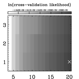
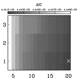
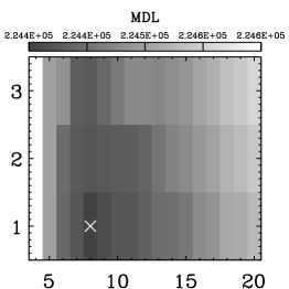
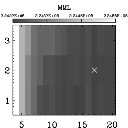
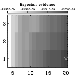
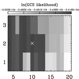
Now that we have introduced the different model selection tests we can apply them to our reconstructed models of the velocity distribution and decide which combination of and is the most suited to describe the velocity distribution. The model selection surfaces for all of the different tests described above are given in Figure 8. In each of the panels the darker values of the density map correspond to models that are preferred by that particular model selection criterion. We see that most of the internal model selection criteria don’t give a definite answer as to the amount of complexity that is warranted by the data, as they prefer models of ever increasing complexity. Only the MDL criterion, which, as can be seen from equation (20), is very harsh on the introduction of extra parameters, seems to turn over around a value of .
The one test that does have a clear preference is the test based on the radial velocities from the GCS. This model selection criterion clearly prefers models with a value for the regularization parameter of 4 km2 s-2, and among those models it prefers a moderate value of = 10. Adding more and more components to the mixture makes the predictions of the radial velocities progressively worse. Since this test with the external radial velocities is arguably the most stringent, we will adopt from now on the values and km2 s-2 as fiducial values. The parameters of the best fit model with these parameters are given in Table 1. We will discuss the features of this reconstruction of the velocity distribution extensively below.
That our fiducial model does a good job of predicting the radial velocities—i.e., it does not just do a better job than the other models—can be seen from Figure 9, in which the distribution of the quantiles of the predicted radial velocity distribution at which the observed value of the radial velocity is found is shown: For each radial velocity from the GCS we integrated the predicted radial velocity distribution up to the observed value of the radial velocity and plotted the distribution of the quantiles thus obtained. If our predicted distribution function for the radial velocities was absolutely perfect this curve would be completely flat. The fact that it rises slightly at the ends of the interval is because our velocity distribution does a bad job of predicting the radial velocities of high-velocity stars. However, for intermediate and low velocity stars our predicted radial velocities are in good agreement with the observations.
In the next section we discuss in more detail how well our reconstruction of the velocity distribution predicts the radial velocities of the GCS stars, which will allow us to assess the usefullness of complementary radial velocity surveys to upcoming astrometric surveys for the purpose of establishing the statistical properties of the kinematics of the stars.
Section 5 Information content of the predicted radial velocities
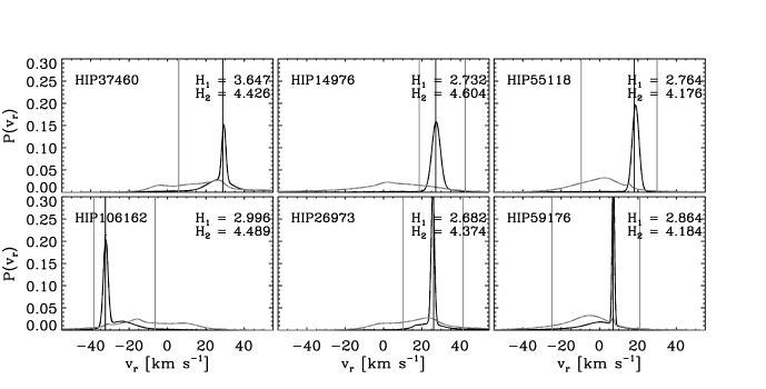
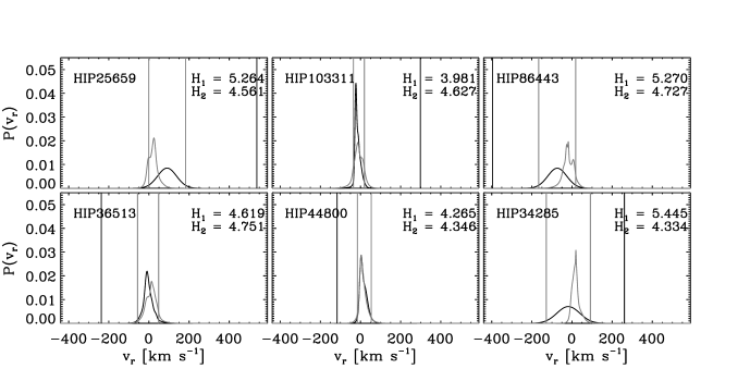
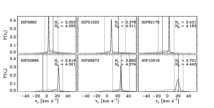
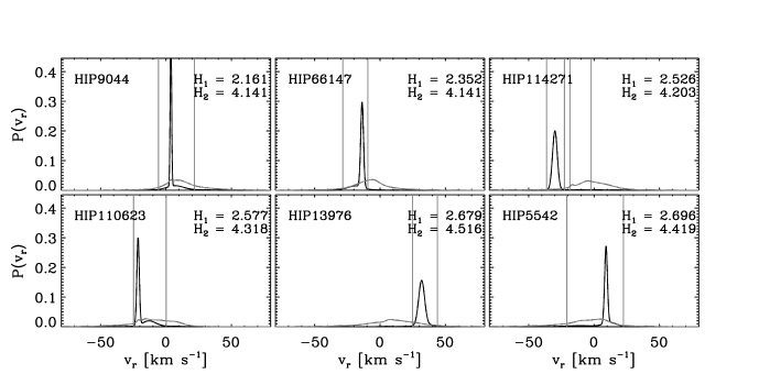
To start off the discussion on how well the reconstructed velocity distribution predicts the radial velocities of stars in the GCS we draw attention to some of the best predictions in Figure 10. Shown are the six “best” predictions of radial velocities, where by best we mean that the probabilities of the observed radial velocities given the model and their tangential velocities are very large for these stars. What we see are very narrow predicted distributions, with a width of only a few km s-1, and the observed radial velocities are right at the peak of the distribution. The predicted distributions of these radial velocities given only their position, which are shown in gray, are very broad, such that the tangential velocities really pin down the value of the radial velocity, as can also be seen by the large difference in entropy between these two distributions. Thus, in these cases the radial velocity of the star does not provide much extra information, as its location in velocity space can be constrained tightly from its tangential velocity alone.
However, among the individual predictions we make there are also some impressive failures. The six “worst” predictions are shown in Figure 11, where worst means here that these radial velocities have very small probabilities given the model and their tangential velocities. All of these bad predictions are for very high velocity stars and it is no surprise that we cannot accurately predict the radial velocities of these stars, since the sample of stars that we used to reconstruct the velocity distribution does not sample the high velocity stars, e.g., halo stars, well. Keeping in mind the range in radial velocity in these plots, one can see that the predicted distributions are very broad, with a typical width of 100 km s-1, and that the addition of the tangential velocities to the positions of these stars in order to make the prediction does not help to zero in on the value of the radial velocity. Indeed, in most cases the entropy of the two predicted distributions are about the same, and in a few cases the entropy of the probability distribution for the radial velocity given the tangential velocity is actually larger than the entropy of the predicted distribution given the position of the star alone, indicating that our model of the velocity distribution really has no clue about the value of the radial velocity for these stars.
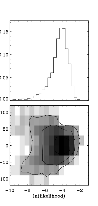
In Figure 12 we look at the probability of all of the radial velocities given the model and their tangential velocities for the full sample of radial velocities from the GCS. A long tail towards small probabilities stands out in this figure. The stars with radial velocities with the lowest probability making up this tail are distributed all over the sky such that this tail does not indicate that our deconvolution technique has failed to reconstruct the velocity distribution in a particular direction (or set of directions) on the sky. Inspecting the correlation between the probability of the observed radial velocity given the model and the value of the radial velocity shows that the tail is a consequence of our inability to predict the radial velocities of very high velocity stars, as we already established above. Ignoring these high-velocity stars, we see that on average the probability of an observed radial velocity given the model of the velocity distribution is . In the language of information theory, this means that an observed radial velocity adds about 4 nats 5.8 bits of information to our knowledge.
Another important measure of the information contained in our predicted probability distributions for the radial velocities is the entropy of the distribution. Broad probability distributions have large entropies and low information content: They do not make a very definite prediction for the radial velocity of a star. Very narrow, sharp distribution functions have low entropy and do make tight predictions for the radial velocities. In Figure 13 the six “tightest”, or lowest entropy, predicted probability distributions for the radial velocities are shown. The probability distributions given the tangential velocities are all very sharp, with typical widths of approximately 5 km s-1 for these tightest predictions. The entropies of these predictions based on the tangential velocities of the stars are all much smaller than the entropies of the radial velocity distributions based on the position alone, which again means that the tangential velocities together with the model of the velocity distribution strongly constrain the value of the radial velocity of these stars. For this sample of the six tightest predictions, the predicted radial velocities do not agree particularly well with the observed radial velocities. In many cases the observed radial velocity is located in a region of the probability distribution that is quite far removed from the peak of the distribution, although in most cases there is still a non-vanishing mass of the probability distribution associated with the region of the observed radial velocity. This clearly indicates that a knowledge of the tangential velocities alone is not enough to reliably predict the radial velocity of a star, and that the tangential velocity of a star can be very misleading in this respect.
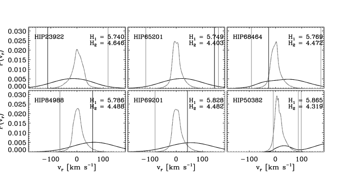
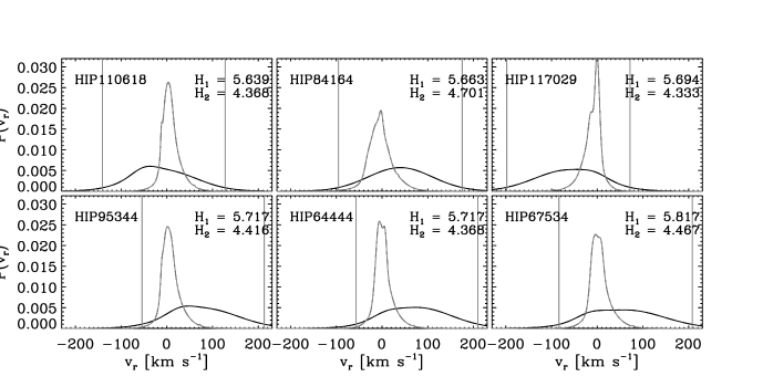
The six “widest”, or highest entropy, predicted probability distributions are shown in Figure 14. The predictions for the radial velocitites of these stars based on the position alone are all informative, so these stars are such that the direction in which they are observed has significant substructure that could potentially pinpoint the velocity of the star based on the tangential velocities of the star alone, but the measured tangential velocity of the star does not indicate that the star is part of any of the clumps in this direction. Most of the observed radial velocities indeed do not correspond to any of the peaks in the predicted distribution in the direction of the star. The probabilities of the radial velocities of these stars given the model and their tangential velocity is not particularly low compared to the average probability of a radial velocity. Therefore, we can conclude that most of these stars are probably part of the background population of stars, although some, but not all, are also high-velocity stars.
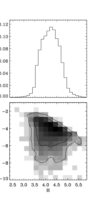
In Figure 15 the distribution of the entropies of the predicted probability distribution for the radial velocities based on their tangential velocities is shown together with a two-dimensional histogram of the entropies and the probabilities of the observed radial velocities. The distribution of entropies is fairly symmetrical around the mean value corresponding to a moderately informative distribution. The bottom panel shows a hint of an anti-correlation between the entropy of the predicted distribution and the probability of the observed radial velocity: More informative predicted distributions have a slight preference toward higher probabilities of the observed radial velocity given this distribution. This indicates that when the model together with the observed tangential velocity makes an informative prediction, corresponding to a low entropy, this prediction more often than not turns out to have been a good prediction. However, the broad swath of average entropies with low probabilities of the observed radial velocity again indicates that our predicted radial velocities lack the accuracy to make the observations of radial velocities obsolete in this context.
As a final comparison of our predictions for the distributions of the radial velocities we look at the distribution of radial velocities in different patches of the sky. In Figure 16 the predicted and observed distribution of radial velocities is shown for four different directions: the direction towards the poles of the ecliptic and three random directions. The observed distribution of radial velocities is obtained by binning the radial velocities of stars from the GCS. The predicted distribution of radial velocities is the prediction based on the central and of each patch, as given in equation (28). The predicted and observed distributions agree well for all of these patches, as one can readily see by eye. Slight offsets between the observed and predicted distributions are inevitable because of the large range in both and that we have to give to the patches in order to get a reasonable number of observed stars in a patch: the distribution in a patch is non-uniform and this moves the observed distribution away from the predicted distribution in some cases. However, even in such cases, the shape of the predicted and observed distributions agrees well. We refrain from making any quantitive statements about the agreement between the observed and theoretical distribution, e.g., by using the Kolmogorov–Smirnov statistic for testing whether observations were drawn from a given distribution, because of these difficulties in the interpretation of the agreement between observed and predicted distribution. However, this comparison does show that our reconstructed velocity field gets the major properties of the distribution of the radial velocities right. Thus, we see that we can predict the bulk properties of the radial velocities from observations of the tangential velocities alone. We stress the importance of the full sky-coverage of our sample of tangential velocities in this respect: Under the assumption of a homogeneous velocity distribution in this volume around the Sun we need at least sterradian to sample all directions of the velocity distribution from the tangential velocities alone.
Section 6 Predictions for non-GCS stars
Since we can make detailed predictions for the radial velocity of any star in the Solar neighborhood, whether we know its tangential velocity or not, we can look at the stars from our sample from Hipparcos which do not have a measured radial velocity, and identify particularly interesting stars from the point of view of their radial velocity. For instance, we can calculate the entropy of the predicted distribution for the radial velocity of a star and find the stars for which our prediction is particularly informative. In Figure 17 the six most informative predictions, i.e., lowest entropy predicted probability distributions for the radial velocity, are shown for stars in our Hipparcos sample without radial velocity in the GCS. The predicted distribution for the radial velocity of these stars are all highly peaked at one particular value for the radial velocity.
A detailed list of the properties of the stars with the most informative predicted radial velocity distributions is given in Table 2. This table lists the stars sorted by the value of the entropy of their predicted probability distributions for the radial velocity and gives the maximum likelihood estimate of the radial velocity as well as 95 percent upper and lower limits on the radial velocity derived from the predicted distribution. As discussed in the previous section and shown in Figure 13, these predictions could still be far fom the truth.
A similarly interesting sample of stars are the stars for which the predicted distribution of the radial velocity is very uninformative. The six least informative predictions are shown in Figure 18. As these are stars for which we have essentially no clue about their radial velocity, given the model of the velocity distribution and their tangential velocity, obtaining their radial velocity would be interesting as it would add a substantial amount of knowledge about the velocities of nearby stars. A list of the 25 least informative predictions for stars in the Hipparcos sample used here that have no radial velocity from the GCS is given in Table 3.
Finally, Figure 19 shows the distribution of the entropies of the predicted distributions for all of the stars for which we have no radial velocity. Comparing this distribution to the distribution of the entropies of the predicted radial velocities of stars which do have a measured radial velocity, shown in Figure 15, shows that the information content and its distribution in this sample of unobserved radial velocities is about the same as the information content in the stars that already have measured radial velocities.
Section 7 Discussion
7.1 Why do the different model selection criteria differ?
The analysis of the complexity of the velocity distribution in Section 4.3 showed that there is a large difference in this context between the internal model selection criteria and the external test based on the predictions of our model of the radial velocities of the GCS stars. Because of the importance of this conclusion for the comparison of our results with the amount of structure in the velocity distribution reported in the literature, we would like to understand the discrepancy between the conclusions of internal and external tests of the structure in the velocity distribution.
The first thing to note in this respect is that the specific forms of the internal tests which we have applied are in most cases approximations to the underlying model selection principles. For example, in order to obtain a computationally feasible version of the leave-one-out cross-validation principle we were forced to perform a very restricted fit of the model to each of the leave-one-out subsamples, i.e., we only allowed the best-fit model for each of the leave-one-out subsamples to differ from the global best fit model in the amplitudes of the Gaussian components of the mixture. Similarly, the expression in equation (21) for the message length used in the minimum message length model selection criterion as well as the form given in equation (23) for the Bayesian evidence are only approximations to the true message length and the true Bayesian evidence, respectively, for the Gaussian mixture model for a distribution function. In the case of the approximation to the message length we know that one of the approximations we are making is wrong on some level, since the approximation assumes that the different Gaussian components in the mixture do not overlap significantly, whereas it is obvious from the reconstructions of the velocity distribution in Figure 2 that this is not the case. It is therefore possible that some of these approximations are inappropriate for the current application and that, if this were possible, the application of the true model selection principle would give different results for the amount of complexity in the velocity distribution. However, the fact that most of the internal model selection criteria in Figure 8 behave similarly as a function of the complexity of the model hints at the existence of a deeper reason for the discrepancy between the internal and external model selection tests.
One of the reasons for this discrepancy could be unknown issues with the data. For example, it is possible that significant star–to–star covariances exist in the Hipparcos data. Because of the complexity of the Hipparcos mission it is not immediately obvious that such star–to–star covariances should be small, although much effort has been made in the data reduction process to remove these correlations (e.g., van Leeuwen, 2007a). Unknown correlations between supposedly independent data points can cause internal model selection criteria such as leave-one-out cross validation to overestimate the amount of structure in the velocity distribution function because the “external” check of the velocity distribution found for each jackknife-subsample with the data point that was left out fails, since if the data point that was left out is correlated with other data points it was not really left out of the data set. Other internal model selection criteria which we used above will be similarly affected, as, for instance, unknown star–to–star covariances will lead to an overestimate of the message length in the minimum message length criterion which could easily move the minimum of the message length function towards higher complexities.
Another possible issue with the data is a difference between the assumed, Gaussian error distribution for the Hipparcos parallaxes and proper motions and the true error distribution, either because of underestimates of the width of the error distribution or through non-Gaussianities. Both of these possibilities would generically lead to a a larger amount of structure in the velocity distribution than the actual amount of structure.
Rather than issues with the data there could be problems with the model for the velocity distribution which we use here. If the model is inadequate, i.e., if the true velocity distribution does not lie in or even near the space of allowed models, then model selection will fail in general, because one is choosing between different models which are all bad representations of the true velocity field. In that situation it is natural to find that the model selection tests prefer models of increasing complexity, because, e.g., adding a component could substantially increase the goodness of the fit over the model with less complexity, while still being very far from the truth. However, it seems unlikely that the true velocity distribution is very far removed from being adequately described by a mixture of Gaussian distributions model, since the velocity distribution of a relaxed population of stars is approximately Gaussian and dispersing star clusters should also be well-described by approximately Gaussian velocity distributions. However, if the structure in the velocity distribution is caused by resonances, or if the projection onto velocity space of partially phase-mixed structures in the six-dimensional phase-space distribution of stars gives rise to singularities (Tremaine, 1999), such as folds or cusps, then the mixture of Gaussian distributions model might be inadequate.
Although it is hard to assess the role played by the different effects described in this subsection in determining the outcome of the model selection tests, it should be clear that an external model selection tests will be affected much more weakly by all of them. The validation of the reconstruction of the velocity distribution by the radial velocities of GCS stars does not require us to make any approximations, since we can predict straightforwardly the probability distribution for the radial velocity of each GCS star and compare it to the observed radial velocity. The external test is not plagued by any unknown issues with the Hipparcos data since the radial velocity data is completely separate from the Hipparcos data (as we project our model of the velocity distribution onto the space of the radial velocity for each GCS star rather than combining the GCS radial velocity with the tangential velocities measured by Hipparcos to form the three-dimensional velocity ). The external test also provides a robust check of the adequacy of the model space which we consider, as the radial velocities would all be very improbable if the model were very far from the truth. We saw that this was not the case in Section 5. The external test applied here is therefore the most conservative model selection test. Any structure in the velocity distribution that passes this conservative test can therefore be reliably considered real. This does not, however, exclude the existence of more structure in the velocity distribution, although if more structure exists, it must be at much lower significance in the Hipparcos/GCS data than the structure recovered here.
7.2 The complexity of the velocity distribution
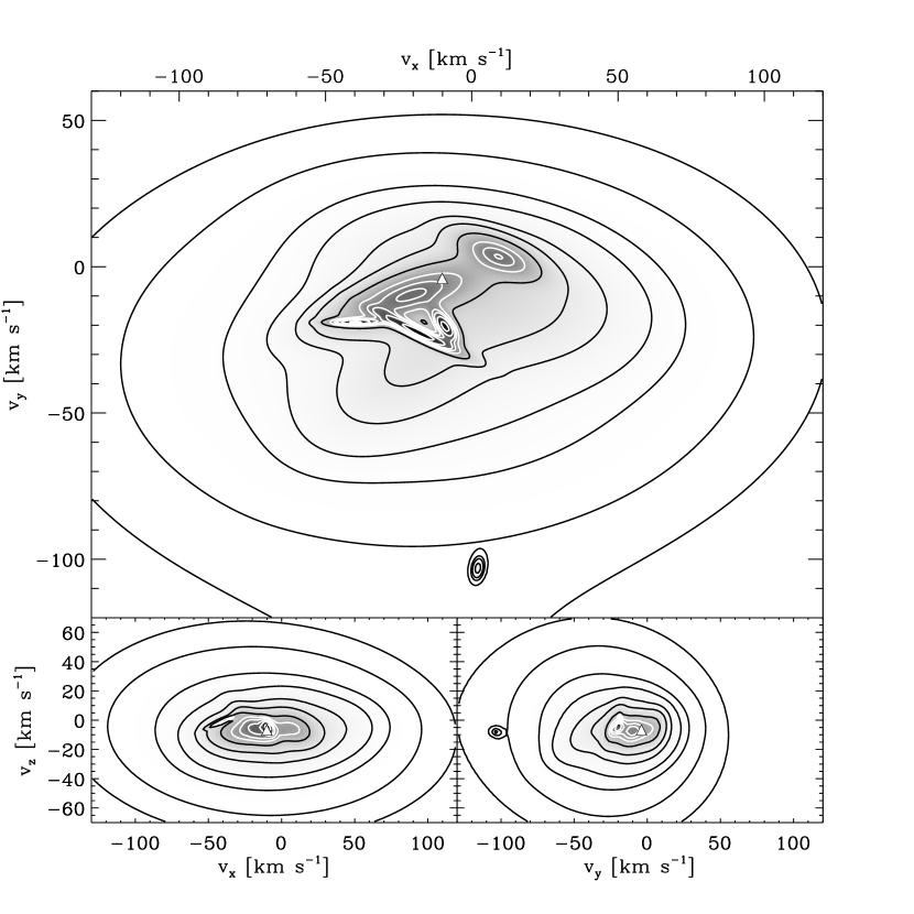
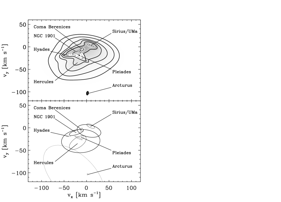
As we discussed in Section 4.3, our model selection criterion based on the GCS radial velocities shows a clear preference for a model of the velocity distribution with only a modest amount of complexity. The preferred model consists of ten Gaussian components such that only a limited number of clumps are apparent in the reconstructed velocity distribution, which is shown in Figure 20. This stands in sharp contrast with many of the analyses of the velocity distribution in recent years, which have revealed an increasing amount of structure and clumps in the velocity distribution.
One of the first comprehensive studies of the velocity distribution based on Hipparcos data showed lots of structures in the – projection of the velocity distribution (Dehnen, 1998). Subsequent analyses turned up even more substructures, in the form of branches (Skuljan et al., 1999) and an ever-increasing number of clumps, or moving groups candidates (Antoja et al., 2008; Zhao et al., 2009). Using much of the same data we are unable to confirm much of the perceived structure. A few reasons are responsible for this: (1) our rigorous, conservative model selection procedure and (2) the attention we paid to the smallest scales on which we can reliably detect substructures given our data.
Comparing the criteria which we used to decide on the best model of the velocity distribution among many models characterized by different levels of complexity shows that internal tests of the complexity of the velocity distribution, such as the criteria that have been applied in all of the recent studies, give very different answers than model selection criteria depending on an external data set (see also the discussion in the previous subsection). Much of the evidence for the existence of structure in the velocity distribution in the past has hinged upon the detection of similar structures in different subsamples of the data, e.g., color subsamples (Dehnen, 1998), or on the detection of the same features across different analysis techniques. All of these different procedures for establishing the reality of the complexity seen in the data all point towards a maximal amount of structure in the velocity distribution, to such an extent that every little wiggle (Dehnen, 1998) or overdensity in the velocity distribution (Zhao et al., 2009) is perceived as real. The internal model selection criteria which we have applied here also lead to the same conclusion: most of them prefer the models with the most complexity. However, the external model selection criterion which we applied, predicting the radial velocities of a large sample of stars and preferring the model which best predicts these radial velocities, is arguably more stringent than any internal test could ever be and clearly gives a very different answer than the internal tests. This test of predicting the radial velocities and comparing them to the observations unambiguously points toward a model with only a modest amount of complexity.
A second, somewhat less important, reason for the discrepancy between our results and some recent findings is that we explicitly considered the smallest scales on which we could reliably detect structure in the distribution of velocities, through our use of a renormalization parameter for the covariances of the components of the distribution, which roughly sets the scale of the smallest structures we could find. We applied our model selection criteria to find the best value of this parameter as well and found a clear preference for a value of 4 km2 s-2 over smaller values. Thus, testing our models of the velocity distribution on the radial velocities from the GCS shows that on average we cannot trust structures on scales smaller than 2 km s-1. Thus it is unsurprising that we cannot recover structures in the velocity distribution found by techniques such as wavelet analysis which manually or semi-automatically set the scale of the structures they want to find to values of 1 km s-1 and smaller (Antoja et al., 2008; Zhao et al., 2009). As has been remarked before (Dehnen, 1998) and as our analysis also shows, structures on scales of a few km s-1 are likely to be spurious.
7.3 The structure of the velocity distribution
We will discuss the properties of the reconstructed velocity distribution in a separate paper (J. Bovy, D. W. Hogg, & S. T. Roweis, 2009, in preparation), in which we will also look in detail at the composition of the different clumps which we identify in the velocity distribution, but here we briefly discuss the main features of the velocity distribution shown in Figure 20.
Most of the features of the velocity distribution are in the – projection of the three-dimensional velocity distribution. This is as expected, since phase mixing in the vertical direction is much more efficient than in the horizontal direction because the potential in the vertical direction varies more rapidly with position than the potential in the horizontal direction in the Solar neighborhood. The projection in the – plane could be well approximated by a single Gaussian distribution, as expected for a well-mixed distribution of stars. The projection in the – plane, except for a structure at large negative which we discuss below, also corresponds to an approximately phase-mixed distribution function, which is skewed because of the combined effect of the exponential density profile of the stellar disk and the decreasing velocity dispersion with Galactocentric radius in the disk (Binney & Tremaine, 2008).
In the – plane we clearly see the most prominent moving groups in their expected places. In Figure 21 we show the projection of the velocity distribution in the – plane with the moving groups indicated. Also shown is a visual representation of the individual Gaussian components of the velocity distribution in our reconstruction: The location, covariance structure, and weight of each component in the mixture is represented by 1–sigma contours around the center of each Gaussian component with the linewidth indicating the relative weight of the different components. Although we stress that in the mixture of Gaussians approach to density esimation the individual Gaussian components are meaningless, it is immediately clear that there is a good and unambiguous correspondence between the individual components and the modes of the distribution, which are typically interpreted as moving groups. Therefore, in the following we will use the Gaussian components as proxies for the peaks of the distribution function. The Gaussian component with the largest weight does not correspond to a peak in the velocity distribution and has a large dispersion. Therefore, it is most probably part of the background distribution. The moving group with the largest weight (as judged by the amplitude of the corresponding Gaussian component in the mixture, see Table 1) is located at -23 km s-1, -10 km s-1, although it is unclear at this point whether we can attribute all of the weight of this component to the moving group or whether part of this component should be identified with the background distribution of stars. This group is known as NGC 1901 and it has been known for a long time. The Coma Berenices moving group is typically found in this region as well; we cannot naively associate a component of the mixture of Gaussians with its fiducial location at -10 km s-1, -5 km s-1. However, looking at its location in Figure 21, especially in the bottom panel, we see that the region where the Coma Berenices moving group is typically found is a part of the velocity distribution where three of the Gaussian components with large weights in the mixture overlap. The overdensity that this overlap gives rise to might indicate the presence of the Coma Berenices moving group. We will come back to this question in paper II, where we will perform a more sophisticated analysis than naively associating components in the mixture with moving groups of the velocity distribution and its substructures.
The Hercules group, which is not singled out by a contour in Figure 20 but is nevertheless present in our best fit model of the velocity distribution, is found at -20 km s-1, -33 km s-1. Whether there is a valley between the Hercules group and the main extent of the velocity distribution, is not entirely clear here, although it does seem like the Hercules group merely sits on top of the background distribution like all of the other moving groups. Following the descending order of the weights of the Gaussian components, the Sirius moving group, located at 9 km s-1, 4 km s-1 also stands out clearly at about the same location that it has been reported at before (e.g. Dehnen, 1998).
The Hyades and Pleiades moving groups are also clearly visible in the velocity distribution: Two components of the mixture of Gaussians are near where the Pleiades is traditionally located, at -15 km s-1, -20 km s-1. That there are two components associated with the Pleiades moving group could mean that there is substructure in the Pleiades moving group which has so far gone unnoticed, or it could indicate that there is a dearth of stars with velocities around -18 km s-1, -19 km s-1, forcing our fit of the velocity distribution as a sum of Gaussian components to include two components at the location of the Pleiades in order to reproduce the lack of stars between the Pleiades moving group, the Hyades moving group, and NGC 1901. More speculatively, this structure is reminiscent of the kind of singularities that can appear when partially phase-mixed structures are projected into a lower-dimensional space (Tremaine, 1999).
The Hyades moving group is also found at its expected location at -40 km s-1, -20 km s-1. Judging by the amplitude of the Gaussian component corresponding to the Hyades moving group, this group only contains about 1.75 percent of the stars in the Solar neighborhood, much less than the other moving groups discussed above.
We find one overdensity far removed from the main part of the velocity distribution. This overdensity corresponds to the Arcturus stream, at 0 km s-1, -105 km s-1. It clearly stands out over the background of stars and can be seen in all of our reconstructions of the velocity distribution with a sufficient number of components, see Figure 2. This group of stars presumably belongs to the thick disk and it has been hypothesized that it has an extragalactic origin (Navarro et al., 2004). From Figure 20 it is clear that it has a very small width in velocity space, and judging by the covariance matrix of the Gaussian component corresponding to the Arcturus group its velocity dispersion is 2–3 km s-1. This small velocity dispersion casts doubts on the extragalactic interpretation of this group. It is in sharp disagreement with the velocity dispersion of 50 km s-1 derived based on a sample of 46 stars believed to be part of the Arcturus stream for which Hipparcos parallaxes and proper motions are available (Navarro et al., 2004). A similar small velocity dispersion as found here has also been reported based on a joint analysis of the GCS data and a sample of metal-poor stars in the Solar neighborhood (Williams et al., 2009; Schuster et al., 2006). The same analysis also found that the Arcturus group is chemically similar to the background thick disk stars, which is inconsistent with the abundance properties of present-day dwarf Spheroidal galaxies, casting further doubt on the interpretation of the Arcturus group as having an extragalactic origin. We will discuss the properties of the Arcturus group further in paper II.
Naively using the weights in the mixture of the components corresponding to the different moving groups shows that many of these groups contain up to 10 percent of the stars in the Solar neighborhood, although the large number of stars that seems to be part of NGC 1901 is probably a consequence of contamination from background stars for this moving group. The weights of the different moving groups are in good agreement with the fractions of different moving groups found by Famaey et al. (2005), although we are able to distinguish between more moving groups than was the case earlier. Assuming that much of the second component of the mixture is caused by the background leads us to the conclusion that 40 percent of the stars in the Solar neighborhood are part of a moving group.
Section 8 Conclusion
Our detailed analysis of the velocity distribution of nearby stars
from Hipparcos data has lead us to the following conclusions:
Performing a very conservative validation of our
reconstruction of the velocity distribution based on
tangential velocities of stars with the radial velocities of a sample
consisting of a similar number of stars shows that the amount of
complexity necessary in our model of the velocity distribution to
provide a good fit to the underlying velocity distribution is
relatively small. Adding more complexity to the model gives better
fits to the distribution of the tangential velocities, but fails to
provide a good fit to the validation set of radial velocities.
Therefore, unlike previous analyses, which validated their models of
the velocity distribution using only internal tests, we conclude that
there is not much evidence in the Hipparcos data of much structure
in the velocity distribution beyond the major, known moving
groups. This does not preclude the existence of more structure in the
velocity distribution of nearby stars, but if more structure exists it
is present at only low significance in the Hipparcos/GCS data
set.
Similarly, the same validation procedure shows that
the smallest scale on which we can reliably identify structure in the
velocity distribution from Hipparcos data is a few km s-1. This
calls into question claims from previous analyses of the Hipparcos data of structure in the velocity distribution at the level of 1 km
s-1.
Our predictions of the radial velocities of
stars based on the model for the velocity distribution shows that we
get the bulk properties of the radial velocities correct using only
the tangential velocities of stars. This indicates that it is unlikely
that the addition of radial velocities to the sample on which we base
the fit would lead to a very different model for the velocity
distribution. This is unsurprising given the full-sky coverage of
Hipparcos and the small spatial extent of our sample.
Predicting probability distributions for individual radial velocities
of stars based on the model of the velocity distribution and the
stars’s tangential velocities and comparing them to the observed
radial velocities shows that there is still quite a bit of information
on average in the radial velocities: The predicted probability
distributions have relatively high entropy, i.e., they are not very
narrow in general, and the probability of the observed radial
velocities are rather small on average. In this context, each radial
velocity provides on average 6 bits of extra
information.
A preliminary investigation of the properties
of the velocity distribution shows that we recover all of the major
moving groups at the approximate locations at which they have been
found in the past: We find strong evidence for the Sirius/Ursa Major
group, the Hyades/Pleiades moving groups, the Hercules moving group,
the NGC 1901 group, and a thick disk stream, the Arcturus group. One
new feature that shows up in our reconstruction of the velocity
distribution is a dearth of stars between the Pleiades, the Hyades,
and the NGC 1901 moving groups, although it is unclear at the moment
whether the lack of stars in this region is a real underdensity or
whether it indicates substructure in the Pleiades moving group. A more
careful analysis of the reconstructed velocity distribution is
necessary to to distinguish between these two possibilities. We also
find that the Arcturus groups is kinematically cold, which calls its
interpretation as originating from the debris of a disrupted satellite
into question.
A first look at the weights of the
different moving groups in the velocity distribution shows that about
40 percent of the stars in the Solar neighborhood is part of a moving
group. Each of the major moving groups holds up to 10 percent of the
stars.
As a result of our semi-parametric fit to the
velocity distribution, we have found a simple, explicit model for the
velocity distribution, given in Table 1, which can be
used in theoretical studies and as the basis for a comparison of the
velocity distribution found here to that found by other methods.
References
- Akaike (1974) Akaike, H. 1974, IEEE Transactions on Automatic Control, 19, 716
- Antoja et al. (2008) Antoja, T., Figueras, F., Fernández, D., & Torra, J. 2008, A&A, 490, 135
- Asiain et al. (1999) Asiain, R., Figueras, F., Torra, J., & Chen, B. 1999, A&A, 341, 427
- Baade (1944) Baade, W. 1944, ApJ, 100, 137
- Baade (1958) Baade, W. 1958, in Stellar Populations: Proceedings of the conference sponsored by the Pontifical Academy of Science and the Vatican Observatory, May 20-28, 1957, ed. D. J. K. O’Connell (Amsterdam: North-Holland Pub. Co.), 3
- Bahcall & Soneira (1980) Bahcall, J. N. & Soneira, R. M. 1980, ApJS, 44, 73
- Bahcall & Soneira (1984) Bahcall, J. N. & Soneira, R. M. 1984, ApJS, 55, 67
- Bienaymé (1999) Bienaymé, O. 1999, A&A, 341, 86
- Binney & Tremaine (2008) Binney, J. & Tremaine, S. 2008, Galactic Dynamics: Second Edition (Princeton University Press)
- Binney et al. (1997) Binney, J. J., Dehnen, W., Houk, N., Murray, C. A., & Penston, M. J. 1997, in ESA Special Publication, Vol. 402, Hipparcos - Venice ’97, 473
- Blaauw et al. (1960) Blaauw, A., Gum, C. S., Pawsey, J. L., & Westerhout, G. 1960, MNRAS, 121, 123
- Boesgaard & Budge (1988) Boesgaard, A. M. & Budge, K. G. 1988, ApJ, 332, 410
- Boss (1911) Boss, B. 1911, AJ, 27, 33
- Boss (1908) Boss, L. 1908, AJ, 26, 31
- Bovy et al. (2009) Bovy, J., Hogg, D. W., & Roweis, S. T. 2009, arXiv:0905.2979 [stat.ME]
- Boyle & McClure (1975) Boyle, R. J. & McClure, R. D. 1975, PASP, 87, 17
- Bozdogan (1983) Bozdogan, H. 1983, Determining the number of component clusters in the standard multivariate normal mixture model using model-selection criteria, Tech. rep., TR UIC/DQM/A83-1, Quantitative Methods Dept., University of Illinois
- Breger (1968) Breger, M. 1968, PASP, 80, 578
- Cabrera-Caño & Alfaro (1990) Cabrera-Caño, J. & Alfaro, E. J. 1990, A&A, 235, 94
- Chaudhuri (1940) Chaudhuri, P. C. 1940, MNRAS, 100, 574
- Chen et al. (1997) Chen, B., Asiain, R., Figueras, F., & Torra, J. 1997, A&A, 318, 29
- Chereul et al. (1998) Chereul, E., Creze, M., & Bienayme, O. 1998, A&A, 340, 384
- Chereul et al. (1999) Chereul, E., Crézé, M., & Bienaymé, O. 1999, A&AS, 135, 5
- Conway & Sloane (1992) Conway, J. H. & Sloane, N. J. A. 1992, Sphere Packings, Lattices and Groups (London: Springer-Verlag)
- Dehnen (1998) Dehnen, W. 1998, AJ, 115, 2384
- Dehnen & Binney (1998) Dehnen, W. & Binney, J. J. 1998, MNRAS, 298, 387
- Dempster et al. (1977) Dempster, A. P., Laird, N. M., & Rubin, D. B. 1977, Journal of the Royal Statistical Society. Series B (Methodological), 39, 1
- Eddington (1910) Eddington, A. S. 1910, MNRAS, 71, 43
- Eggen (1958) Eggen, O. J. 1958, MNRAS, 118, 154
- Eggen (1959a) Eggen, O. J. 1959a, The Observatory, 79, 182
- Eggen (1959b) Eggen, O. J. 1959b, The Observatory, 79, 88
- Eggen (1964) Eggen, O. J. 1964, Roy. Greenwich Obs. Bull., 84, 111
- Eggen (1965) Eggen, O. J. 1965, The Observatory, 85, 191
- Eggen (1969) Eggen, O. J. 1969, PASP, 81, 553
- Eggen (1970) Eggen, O. J. 1970, PASP, 82, 99
- Eggen (1971a) Eggen, O. J. 1971a, PASP, 83, 271
- Eggen (1971b) Eggen, O. J. 1971b, PASP, 83, 251
- Eggen (1978) Eggen, O. J. 1978, ApJ, 222, 203
- Eggen (1983) Eggen, O. J. 1983, AJ, 88, 813
- Eggen (1986) Eggen, O. J. 1986, AJ, 92, 910
- Eggen & Sandage (1959) Eggen, O. J. & Sandage, A. R. 1959, MNRAS, 119, 255
- ESA (1997) ESA. 1997, The Hipparcos and Tycho Catalogues (Noordwijk: ESA: ESA SP-1200)
- Famaey et al. (2005) Famaey, B., Jorissen, A., Luri, X., Mayor, M., Udry, S., Dejonghe, H., & Turon, C. 2005, A&A, 430, 165
- Figueras et al. (1997) Figueras, F., Gomez, A. E., Asiain, R., Chen, B., Comeron, F., Grenier, S., Lebreton, Y., Moreno, M., Sabas, V., & Torra, J. 1997, in ESA Special Publication, Vol. 402, Hipparcos - Venice ’97, 519–524
- Francis & Anderson (2009) Francis, C. & Anderson, E. 2009, arXiv:0901.3503 [astro-ph]
- Gelman et al. (2000) Gelman, A., Carlin, J. B., Stern, H. S., & Rubin, D. B. 2000, Bayesian Data Analysis (Chapman & Hall/CRC)
- Gerbaldi et al. (1989) Gerbaldi, M. et al. 1989, ESO Messenger, 56, 12
- Ghigna et al. (1998) Ghigna, S., Moore, B., Governato, F., Lake, G., Quinn, T., & Stadel, J. 1998, MNRAS, 300, 146
- Gilmore & Reid (1983) Gilmore, G. & Reid, N. 1983, MNRAS, 202, 1025
- Gomez et al. (1990) Gomez, A. E., Delhaye, J., Grenier, S., Jaschek, C., Arenou, F., & Jaschek, M. 1990, A&A, 236, 95
- Grenier et al. (1985) Grenier, S., Gomez, A. E., Jaschek, C., Jaschek, M., & Heck, A. 1985, A&A, 145, 331
- Grünwald (2007) Grünwald, P. D. 2007, The minimum description length principle (Cambridge, Massachusetts: MIT Press)
- Helmi et al. (2003) Helmi, A., White, S. D. M., & Springel, V. 2003, MNRAS, 339, 834
- Hertzsprung (1909) Hertzsprung, E. 1909, ApJ, 30, 135
- Hogg et al. (2005) Hogg, D. W., Blanton, M. R., Roweis, S. T., & Johnston, K. V. 2005, ApJ, 629, 268
- Ivezić et al. (2008) Ivezić, Ž. et al. 2008, ApJ, 684, 287
- Johnston (1998) Johnston, K. V. 1998, ApJ, 495, 297
- Kapteyn (1905) Kapteyn, J. C. 1905, British Assoc. Adv. Sci. Rep., Sec. A, 257
- Kapteyn (1914) Kapteyn, J. C. 1914, ApJ, 40, 43
- Kolmogorov (1965) Kolmogorov, A. N. 1965, Problems. Inform. Transmission, 1, 1
- Koposov et al. (2009) Koposov, S. E., Yoo, J., Rix, H.-W., Weinberg, D. H., Macciò, A. V., & Escudé, J. M. 2009, ApJ, 696, 2179
- Koposov et al. (2008) Koposov, S. E. et al. 2008, ApJ, 686, 279
- Luri et al. (1996) Luri, X., Mennessier, M. O., Torra, J., & Figueras, F. 1996, A&AS, 117, 405
- Mädler (1846) Mädler, J. H. 1846, AN, 24, 213
- Mädler (1847) Mädler, J. H. 1847, Untersuchungen über die Fixstern-systeme (Lepizig: Mitau)
- McDonald & Hearnshaw (1983) McDonald, A. R. E. & Hearnshaw, J. B. 1983, MNRAS, 204, 841
- Murenzi (1989) Murenzi, R. 1989, in Wavelets. Time-Frequency Methods and Phase Space, ed. J.-M. Combes, A. Grossmann, & P. Tchamitchian, 239–+
- Navarro et al. (2004) Navarro, J. F., Helmi, A., & Freeman, K. C. 2004, ApJ, 601, L43
- Nordström et al. (2004) Nordström, B., Mayor, M., Andersen, J., Holmberg, J., Pont, F., Jørgensen, B. R., Olsen, E. H., Udry, S., & Mowlavi, N. 2004, A&A, 418, 989
- Ogorodnikov & Latyshev (1968) Ogorodnikov, K. F. & Latyshev, I. N. 1968, Soviet Astronomy, 12, 279
- Ogorodnikov & Latyshev (1970) Ogorodnikov, K. F. & Latyshev, I. N. 1970, Soviet Astronomy, 13, 934
- Oliver & Baxter (1994) Oliver, J. J. & Baxter, R. A. 1994, MML and Bayesianism: Similarities and Differences, Tech. Rep. Tech Report 206, Dept. of Computer Science, Monash University, Clayton, Vic. 3168, Australia
- Oliver et al. (1996) Oliver, J. J. O., Baxter, R. A., & Wallace, C. S. 1996, in In Machine Learning: Proceedings of the Thirteenth International Conference (ICML 96 (Morgan Kaufmann Publishers), 364
- Oort (1958) Oort, J. H. 1958, in Stellar Populations: Proceedings of the conference sponsored by the Pontifical Academy of Science and the Vatican Observatory, May 20-28, 1957, ed. D. J. K. O’Connell (Amsterdam: North-Holland Pub. Co.), 515
- Ormoneit & Tresp (1996) Ormoneit, D. & Tresp, V. 1996, in Advances in Neural Information Processing Systems 8, NIPS, Denver,CO, November 27-30, 1995, ed. D. S. Touretzky, M. Mozer, & M. E. Hasselmo (MIT Press)
- Perryman et al. (2001) Perryman, M. A. C. et al. 2001, A&A, 369, 339
- Plummer (1913) Plummer, H. C. 1913, MNRAS, 73, 492
- Proctor (1869) Proctor, R. A. 1869, Proc. Roy. Soc. London, 18, 169
- Proust & Foy (1988) Proust, D. & Foy, R. 1988, Ap&SS, 145, 61
- Rasmuson (1921) Rasmuson, N. H. 1921, Med. Lunds. Obs., Ser. II, No. 26
- Rissanen (1978) Rissanen, J. 1978, Automatica, 14, 465
- Roberts et al. (1998) Roberts, S. J., Husmeier, D., Rezek, I., & Penny, W. 1998, IEEE Transactions on Pattern Analysis and Machine Intelligence, 20, 1133
- Roman (1949) Roman, N. G. 1949, ApJ, 110, 205
- Roman (1954) Roman, N. G. 1954, AJ, 59, 307
- Russell (1912) Russell, H. N. 1912, AJ, 27, 96
- Schuster et al. (2006) Schuster, W. J., Moitinho, A., Márquez, A., Parrao, L., & Covarrubias, E. 2006, A&A, 445, 939
- Schwarz (1978) Schwarz, G. 1978, Ann. Stat., 6, 461
- Schwarzschild (1907) Schwarzschild, K. 1907, Nachrichten von der Königlichen Gesellschaft der Wissenschaften zu Göttingen, 5, 614
- Schwarzschild (1958) Schwarzschild, M. 1958, in Stellar Populations: Proceedings of the conference sponsored by the Pontifical Academy of Science and the Vatican Observatory, May 20-28, 1957, ed. D. J. K. O’Connell (Amsterdam: North-Holland Pub. Co.), 207
- Silverman (1986) Silverman, B. W. 1986, Density Estimation for Statistics and Data Analysis (Chapman and Hall)
- Simon & Geha (2007) Simon, J. D. & Geha, M. 2007, ApJ, 670, 313
- Skuljan et al. (1999) Skuljan, J., Hearnshaw, J. B., & Cottrell, P. L. 1999, MNRAS, 308, 731
- Slezak et al. (1990) Slezak, E., Bijaoui, A., & Mars, G. 1990, A&A, 227, 301
- Soderblom & Clements (1987) Soderblom, D. R. & Clements, S. D. 1987, AJ, 93, 920
- Soderblom & Mayor (1993) Soderblom, D. R. & Mayor, M. 1993, AJ, 105, 226
- Solomonoff (1964a) Solomonoff, R. 1964a, Information and Control, 7, 1
- Solomonoff (1964b) Solomonoff, R. 1964b, Information and Control, 7, 224
- Soubiran et al. (1990) Soubiran, C., Gomez, A. E., Arenou, F., & Bougeard, M. L. 1990, in Errors, Bias and Uncertainties in Astronomy, ed. C. Jaschek & F. Murtagh, 407–+
- Starck & Murtagh (2006) Starck, J.-L. & Murtagh, F. 2006, Astronomical Image and Data Analysis (Springer)
- Stone (1974) Stone, M. 1974, Journal of the Royal Statistical Society. Series B (Methodological), 36, 111
- Tollerud et al. (2008) Tollerud, E. J., Bullock, J. S., Strigari, L. E., & Willman, B. 2008, ApJ, 688, 277
- Tremaine (1999) Tremaine, S. 1999, MNRAS, 307, 877
- Tuominen & Vilhu (1979) Tuominen, I. V. & Vilhu, O. 1979, in Liege International Astrophysical Colloquia, Vol. 22, Liege International Astrophysical Colloquia, 355–360
- Ueda et al. (1998) Ueda, N., Nakano, R., Ghahramani, Z., & Hinton, G. E. 1998, in Neural Networks for Signal Processing VIII, 1998. Proceedings of the 1998 IEEE Signal Processing Society Workshop, 274
- van Leeuwen (2007a) van Leeuwen, F. 2007a, Astrophysics and Space Science Library, Vol. 250, Hipparcos, the New Reduction of the Raw Data (Springer)
- van Leeuwen (2007b) van Leeuwen, F. 2007b, A&A, 474, 653
- Wallace (2004) Wallace, C. S. 2004, Statistical and inductive inference by minimum message length (Springer)
- Wallace & Boulton (1968) Wallace, C. S. & Boulton, D. M. 1968, Computer Journal, 11, 185
- Wallace & Dowe (1999) Wallace, C. S. & Dowe, D. L. 1999, The Computer Journal, 42, 270
- Wallace & Freeman (1987) Wallace, C. S. & Freeman, P. R. 1987, Journal of the Royal Statistical Society. Series B (Methodological), 49, 240
- Williams et al. (2009) Williams, M. E. K., Freeman, K. C., Helmi, A., & the RAVE collaboration. 2009, in IAU Symposium, ed. J. Andersen, J. Bland-Hawthorn, & B. Nordström, Vol. 254, 139–144
- Williams (1971) Williams, P. M. 1971, MNRAS, 153, 171
- Wilson (1966) Wilson, O. C. 1966, Science, 151, 1487
- Wilson (1932) Wilson, R. E. 1932, AJ, 42, 49
- Windham & Cutler (1992) Windham, M. P. & Cutler, A. 1992, J. Am. Stat. Assoc., 87, 1188
- Zador (1963) Zador, P. L. 1963, PhD thesis, Stanford U.
- Zador (1982) Zador, P. L. 1982, IEEE Trans. Information theory, 28, 139
- Zhao et al. (2009) Zhao, J., Zhao, G., & Chen, Y. 2009, ApJ, 692, L113
| (km s-1) | (km s-1) | (km s-1) | (km2 s-2) | (km2 s-2) | (km2 s-2) | (km2 s-2) | (km2 s-2) | (km2 s-2) | ||||||||||||
|---|---|---|---|---|---|---|---|---|---|---|---|---|---|---|---|---|---|---|---|---|
| 1 | 0. | 2392 | 5. | 54 | -6. | 97 | -9. | 26 | 699. | 85 | 202. | 09 | 143. | 63 | -110. | 88 | 59. | 47 | 25. | 28 |
| 2 | 0. | 2278 | -22. | 72 | -10. | 24 | -7. | 30 | 243. | 91 | 47. | 60 | 40. | 45 | 72. | 78 | 10. | 75 | 10. | 35 |
| 3 | 0. | 2262 | -12. | 92 | -29. | 57 | -7. | 60 | 1836. | 31 | 670. | 79 | 537. | 94 | 56. | 82 | -56. | 14 | -31. | 09 |
| 4 | 0. | 0891 | -19. | 43 | -32. | 90 | -4. | 93 | 354. | 89 | 233. | 08 | 134. | 61 | 166. | 45 | 108. | 90 | 113. | 46 |
| 5 | 0. | 0851 | 9. | 20 | 3. | 89 | -5. | 99 | 77. | 82 | 25. | 69 | 48. | 58 | -28. | 91 | -18. | 81 | 8. | 87 |
| 6 | 0. | 0674 | -17. | 79 | -22. | 69 | -4. | 51 | 68. | 86 | 18. | 16 | 63. | 64 | -32. | 89 | -46. | 90 | 17. | 34 |
| 7 | 0. | 0398 | -9. | 07 | -20. | 50 | -4. | 88 | 9. | 04 | 13. | 47 | 14. | 04 | -7. | 19 | -5. | 56 | 7. | 63 |
| 8 | 0. | 0174 | -40. | 07 | -18. | 92 | 0. | 64 | 30. | 99 | 0. | 64 | 6. | 14 | 0. | 25 | 13. | 15 | 0. | 19 |
| 9 | 0. | 0072 | -28. | 28 | -105. | 62 | 2. | 87 | 4585. | 93 | 4465. | 62 | 3479. | 86 | -2367. | 35 | -328. | 67 | -120. | 78 |
| 10 | 0. | 0009 | 2. | 08 | -103. | 07 | -8. | 20 | 1. | 30 | 4. | 21 | 2. | 67 | 0. | 53 | 0. | 30 | 0. | 49 |
| ID\ref{HIPNUMBERtwo}\ref{HIPNUMBERtwo}footnotemark: | (1991.25) | (1991.25) | \ref{VRtwo}\ref{VRtwo}footnotemark: | \ref{VRLOWERtwo}\ref{VRLOWERtwo}footnotemark: | \ref{VRUPPERtwo}\ref{VRUPPERtwo}footnotemark: | \ref{ENTROPYtwo}\ref{ENTROPYtwo}footnotemark: | ||||
|---|---|---|---|---|---|---|---|---|---|---|
| (h | m | s) | (∘ | ) | (km s-1) | (km s-1) | (km s-1) | |||
| HIP9044………… | 01 | 56 | 31.97 | -60 | 13 | 37.6 | 4 | -7 | 20 | 2.161 |
| HIP66147………. | 13 | 33 | 32.70 | 08 | 35 | 11.5 | -13 | -29 | -10 | 2.352 |
| HIP114271…….. | 23 | 08 | 39.31 | -15 | 03 | 09.4 | -30 | -37 | -2 | 2.526 |
| HIP110623…….. | 22 | 24 | 37.33 | 16 | 53 | 48.8 | -21 | -25 | 0 | 2.577 |
| HIP13976………. | 03 | 00 | 02.62 | 07 | 44 | 58.9 | 32 | 24 | 43 | 2.679 |
| HIP5542………… | 01 | 11 | 05.93 | 55 | 08 | 59.8 | 9 | -22 | 21 | 2.696 |
| HIP60529………. | 12 | 24 | 30.09 | 31 | 16 | 49.1 | 3 | -18 | 8 | 2.703 |
| HIP171………….. | 00 | 02 | 09.65 | 27 | 05 | 04.2 | -75 | -81 | -8 | 2.717 |
| HIP57378………. | 11 | 45 | 48.85 | 06 | 56 | 33.3 | 10 | -11 | 12 | 2.731 |
| HIP9065………… | 01 | 56 | 42.18 | -49 | 24 | 27.5 | 51 | 1 | 55 | 2.735 |
| HIP68801………. | 14 | 05 | 03.83 | 10 | 00 | 48.5 | -20 | -38 | -13 | 2.751 |
| HIP115013…….. | 23 | 17 | 37.80 | -42 | 11 | 29.6 | -14 | -21 | 9 | 2.773 |
| HIP73593………. | 15 | 02 | 33.18 | 16 | 03 | 17.1 | -27 | -45 | -10 | 2.776 |
| HIP12158………. | 02 | 36 | 41.57 | -03 | 09 | 22.6 | 22 | 3 | 37 | 2.821 |
| HIP77358………. | 15 | 47 | 29.41 | -37 | 54 | 56.9 | -27 | -45 | 2 | 2.834 |
| HIP62724………. | 12 | 51 | 12.17 | 19 | 09 | 40.8 | -1 | -24 | 2 | 2.839 |
| HIP106856…….. | 21 | 38 | 31.87 | 05 | 46 | 18.0 | -29 | -34 | -4 | 2.852 |
| HIP115151…….. | 23 | 19 | 28.97 | -70 | 19 | 23.1 | -9 | -23 | 26 | 2.864 |
| HIP45320………. | 09 | 14 | 10.67 | -63 | 41 | 35.8 | 10 | -6 | 48 | 2.869 |
| HIP13511………. | 02 | 54 | 00.97 | -64 | 54 | 00.2 | 6 | -9 | 34 | 2.889 |
| HIP52332………. | 10 | 41 | 40.91 | -45 | 46 | 07.3 | 9 | -16 | 38 | 2.891 |
| HIP109182…….. | 22 | 07 | 03.26 | 34 | 31 | 16.7 | -19 | -37 | 7 | 2.899 |
| HIP70330………. | 14 | 23 | 23.54 | -27 | 49 | 19.3 | 46 | -32 | 49 | 2.906 |
| HIP6686………… | 01 | 25 | 48.60 | 60 | 14 | 07.5 | 10 | -27 | 22 | 2.918 |
| HIP88771………. | 18 | 07 | 21.02 | 09 | 33 | 49.2 | -38 | -52 | -1 | 2.959 |
Note. — Predictions for the radial velocity are based on the velocity density estimate using 10 Gaussians with regularization parameter = 4 km2 s-2, marginalized for the position on the sky of the star and conditioned on the stars’ tangential velocity.
| ID\ref{HIPNUMBERone}\ref{HIPNUMBERone}footnotemark: | (1991.25) | (1991.25) | \ref{VRone}\ref{VRone}footnotemark: | \ref{VRLOWERone}\ref{VRLOWERone}footnotemark: | \ref{VRUPPERone}\ref{VRUPPERone}footnotemark: | \ref{ENTROPYone}\ref{ENTROPYone}footnotemark: | ||||
|---|---|---|---|---|---|---|---|---|---|---|
| (h | m | s) | (∘ | ) | (km s-1) | (km s-1) | (km s-1) | |||
| HIP67534………. | 13 | 50 | 16.63 | -57 | 15 | 40.3 | 57 | -92 | 209 | 5.817 |
| HIP64444………. | 13 | 12 | 32.07 | -34 | 44 | 50.6 | 72 | -65 | 210 | 5.717 |
| HIP95344………. | 19 | 23 | 49.32 | -81 | 32 | 24.9 | 47 | -61 | 216 | 5.717 |
| HIP117029…….. | 23 | 43 | 26.61 | 58 | 04 | 44.9 | -46 | -205 | 71 | 5.694 |
| HIP84164………. | 17 | 12 | 21.95 | -46 | 33 | 40.0 | 40 | -100 | 173 | 5.663 |
| HIP110618…….. | 22 | 24 | 34.39 | -72 | 15 | 13.6 | -37 | -142 | 126 | 5.639 |
| HIP117702…….. | 23 | 52 | 14.21 | -61 | 25 | 23.4 | 61 | -68 | 184 | 5.589 |
| HIP7869………… | 01 | 41 | 14.20 | -67 | 40 | 33.1 | 80 | -44 | 198 | 5.555 |
| HIP117254…….. | 23 | 46 | 32.69 | -41 | 34 | 47.3 | 25 | -98 | 142 | 5.529 |
| HIP63559………. | 13 | 01 | 26.58 | -27 | 22 | 26.5 | -4 | -74 | 171 | 5.503 |
| HIP102862…….. | 20 | 50 | 22.62 | -40 | 36 | 26.6 | -9 | -136 | 99 | 5.503 |
| HIP55988………. | 11 | 28 | 27.91 | 07 | 31 | 12.9 | 61 | -57 | 173 | 5.493 |
| HIP98532………. | 20 | 01 | 00.43 | -12 | 15 | 17.1 | -73 | -176 | 62 | 5.493 |
| HIP111286…….. | 22 | 32 | 40.70 | -65 | 26 | 07.3 | 39 | -73 | 171 | 5.465 |
| HIP76976………. | 15 | 43 | 03.76 | -10 | 55 | 57.9 | 44 | -70 | 152 | 5.451 |
| HIP5549………… | 01 | 11 | 10.39 | -82 | 32 | 54.0 | 27 | -47 | 185 | 5.432 |
| HIP3086………… | 00 | 39 | 12.81 | 03 | 07 | 59.5 | 13 | -130 | 97 | 5.423 |
| HIP78400………. | 16 | 00 | 19.98 | -16 | 31 | 56.6 | -29 | -119 | 92 | 5.395 |
| HIP17671………. | 03 | 47 | 06.05 | -56 | 02 | 29.5 | 42 | -58 | 152 | 5.384 |
| HIP107731…….. | 21 | 49 | 24.76 | -47 | 58 | 35.9 | 19 | -112 | 103 | 5.337 |
| HIP96185………. | 19 | 33 | 27.40 | 33 | 12 | 04.8 | -49 | -185 | 7 | 5.336 |
| HIP99224………. | 20 | 08 | 33.81 | -15 | 43 | 43.7 | -38 | -148 | 43 | 5.302 |
| HIP100792…….. | 20 | 26 | 11.85 | 09 | 27 | 05.2 | -88 | -185 | 4 | 5.293 |
| HIP30439………. | 06 | 23 | 57.61 | -45 | 56 | 52.2 | 60 | -11 | 175 | 5.284 |
| HIP86013………. | 17 | 34 | 43.34 | 06 | 00 | 48.3 | -87 | -182 | 1 | 5.261 |
Note. — Predictions for the radial velocity are based on the velocity density estimate using 10 Gaussians with regularization parameter = 4 km2 s-2, marginalized for the position on the sky of the star and conditioned on the stars’ tangential velocity.
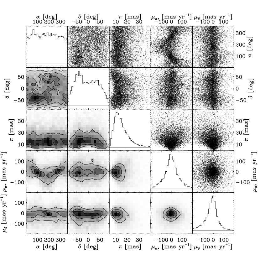
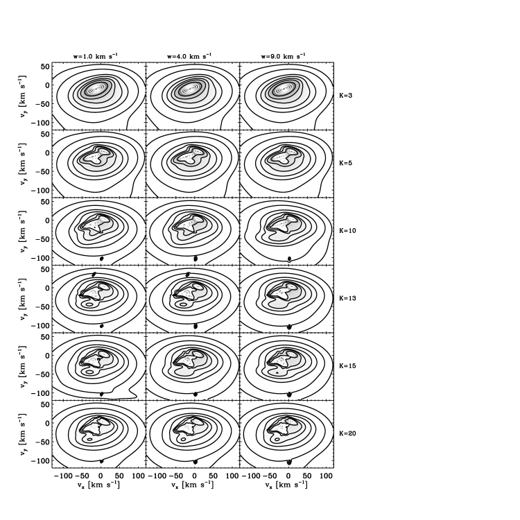
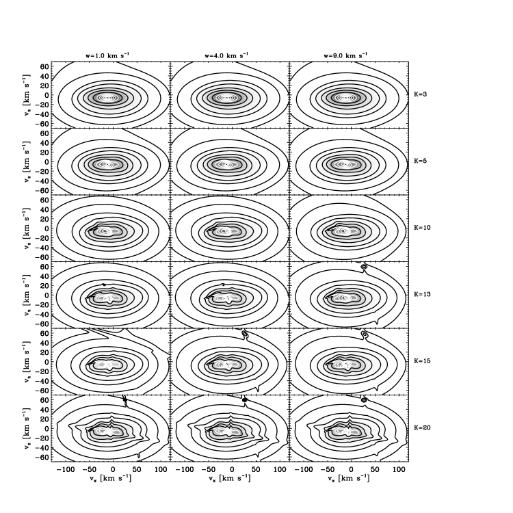
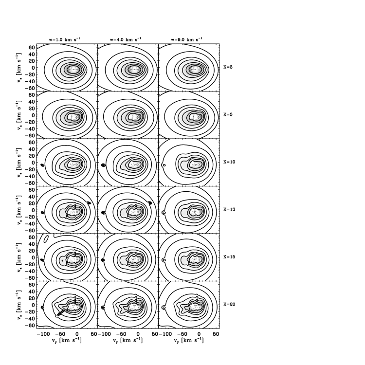
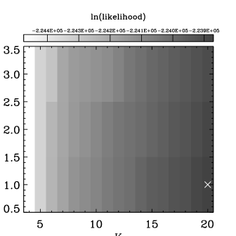
![[Uncaptioned image]](/html/0905.2980/assets/x6.png)
