Tribology of the lubricant quantized-sliding state
Abstract
In the framework of Langevin dynamics, we demonstrate clear evidence of the peculiar quantized sliding state, previously found in a simple 1D boundary lubricated model [Phys. Rev. Lett. 97, 056101 (2006)], for a substantially less idealized 2D description of a confined multi-layer solid lubricant under shear. This dynamical state, marked by a nontrivial “quantized” ratio of the averaged lubricant center-of-mass velocity to the externally imposed sliding speed, is recovered, and shown to be robust against the effects of thermal fluctuations, quenched disorder in the confining substrates, and over a wide range of loading forces. The lubricant softness, setting the width of the propagating solitonic structures, is found to play a major role in promoting in-registry commensurate regions beneficial to this quantized sliding. By evaluating the force instantaneously exerted on the top plate, we find that this quantized sliding represents a dynamical “pinned” state, characterized by significantly low values of the kinetic friction. While the quantized sliding occurs due to solitons being driven gently, the transition to ordinary unpinned sliding regimes can involve lubricant melting due to large shear-induced Joule heating, for example at large speed.
pacs:
68.35.Af, 05.45.Yv, 62.20.Qp, 81.40.Pq, 46.55.+dI Introduction
When a confined lubricant is characterized by a large surface-to-volume ratio, the surface features of the confining walls may strongly affect its tribological properties. If the width of the lubricant film is reduced to a few atomic layers, as in the boundary-sliding regime, the atoms in the film tend generally to be ordered into layers parallel to the bounding substrates.Gao97 ; Tartaglino06 Both numerical simulations and experiments generally conclude that, in such a strongly confined geometry, the film behaves like a solid, even at temperatures significantly higher than its bulk melting temperature.Klein98 In real operative conditions, moreover, the case of “dry” friction is quite exceptional. A physical contact between two solids is generally mediated by so-called “third bodies”, which act like a lubricant film.He99 For crystals sliding on crystals, one may consider the moving contact as characterized schematically by three inherent length scales: the periods of the bottom and top substrates, and the period of the embedded lubricant structure.
The problem of boundary lubricated friction is fascinating both from the fundamental point of view and for applications. Interesting dynamical behaviors, with possible tribologically important implications of an irregular distribution of the lubricant velocity in between the sliding surfaces, have recently been observed in numerical simulations, depending on the “degree” of geometrical incommensurability defining the moving interface.Vanossi06 ; Manini07extended ; Vanossi07PRL ; Manini07PRE The prominent nontrivial feature of those simulation is an asymmetry in the relative sliding velocity of the intermediate lubricating sheet relative to the two substrates. Strikingly, this velocity asymmetry takes an exactly quantized value which is uniquely determined by the incommensurability ratios and is insensitive to all other physical parameters of the model. The occurrence of this surprising and robust regime of motion, giving rise to perfectly flat plateaus in the ratio of the time-averaged lubricant center-of-mass (CM) velocity to the externally imposed relative speed, was ascribed to the intrinsic topological nature of this quantized dynamics. The phenomenon, investigated in detail in a rather idealized 1D geometry,VanossiPRL ; Santoro06 ; Cesaratto07 ; Vanossi07Hyst ; Manini08Erice ; Vanossi08TribInt was explained by the corrugation of a sliding confining wall rigidly dragging the topological solitons (kinks or antikinks) that the embedded lubricant structure forms with the other substrate. Evidence of the existence of this peculiar regime of motion was then confirmed shortly after for a substantially less idealized 2D model of boundary lubrication, where atoms were allowed to move perpendicularly to the sliding direction and interacted via LJ potentials Castelli08Lyon . The solitonic transverse corrugations of the lubricant, propagating inside the film from bottom to top, were observed to favor the kink (or antikink) tendency to pin to the top-layer spatial periodicity, thus strengthening the quantization mechanism.
In this work, we investigate the tribological signature of the quantized-velocity state for such a 2D multi-layer solid lubricant under shear. Its robustness against thermal effects (implemented by means of a standard Langevin approach), quenched disorder in the confining substrates, and over a wide range of loading forces is analyzed in detail. The lubricant softness, setting the width of the propagating solitonic structures, together with the soliton coverage number, is considered in promoting in-registry commensurate regions beneficial to the quantized sliding. Hysteretic termination and kinetic friction are properly evaluated to highlight tribological differences with respect to ordinary unpinned sliding regimes.
The paper is organized as follows. In Sec. II, we summarize the main features of the 2D-implemented tribological confined model, together with the numerical procedure adopted to solve the system of coupled equations describing the dissipative particle dynamics and top plate motion at finite temperatures. Section III is devoted to prove the robustness of the quantized dynamical regime against many physical parameters of the model. In Sec. IV the relative lubricant-lubricant and lubricant-substrate interactions are varied to study the role of the confined film softness. By evaluating the force instantaneously exerted on the advancing plate in Sec. V, we characterize the tribological features of the quantized dynamics and show that it corresponds to significantly low kinetic friction force. The transition towards ordinary sliding regimes can involve lubricant melting due to large shear-induced Joule heating, leading to a higher-friction sliding state. As detailed in Sec. VI, within the framework of our rigid, constant-speed driving, we observe an intermittent stick-slip dynamics, associated to tiny amplitude fluctuations, in the kinetic friction force experienced by the top substrate while in the quantized-velocity state. Discussions and conclusions are given in Sec. VII.
II The 2D confined lubricated model
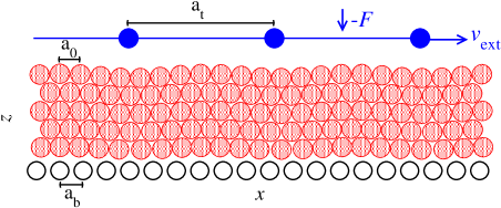
Our system is composed of two rigid walls made of equally-spaced atoms and identical lubricant atoms confined in between, organized in layers, see Fig. 1 where . The lubricant atoms move under the action of pairwise Lennard-Jones (LJ) potentials
| (1) |
describing the reciprocal interactions. The cutoff radius is set at , where .
For the two substrates and the lubricant we assume three different kinds of atoms, and characterize their mutual interactions (, and refer to potential energies for the bottom-lubricant, lubricant-lubricant, and top-lubricant interactions, respectively) with the following LJ radii
| (2) |
which, for simplicity, are set to coincide with the fixed spacings and between neighboring substrate atoms, and the average -separation of two neighboring lubricant atoms, respectively. This restriction is only a matter of convenience, and is not essential to the physics we are describing. These three different periodicities , and define two independent ratios:
| (3) |
the latter of which we take closer to unity, , so that the lubricant is less off-register to the bottom substrate than to the top.
For simplicity, we fix the same LJ interaction energy for all pairwise coupling terms and the same mass of all particles. We take , , and as energy, length, and mass units. This choice defines a set of “natural” model units for all physical quantities: for instance velocities are measured in units of . In the following, all mechanical quantities are expressed implicitly in the respective model units.
The interaction with the other lubricant and sliders’ particles produces a total force acting on the -th lubricant particle, of coordinate , given by
where and are the positions of the top and bottom atoms. By convention, we select the frame of reference where the bottom layer is static, with the atoms located at
| (5) |
The top slider is rigidly driven at a constant horizontal velocity , and can also move vertically (its inertia equals the total mass of its atoms) under the action of the external loading force applied to each particle in that layer and that due to the interaction with the particles in the lubricant layer:
| (6) |
where the equation governing is
| (7) |
To remove the Joule heat, and control the lubricant temperature in this driven system, rather than a Nosé-Hoover thermostat nose-hoover ; Martyna92 as in Ref. Castelli08Lyon, , we use a standard implementation of the Langevin dynamics,Gardiner with the addition of a damping term plus a Gaussian random force to the Newton equations for the lubricant particles. The damping force includes the contributions of the energy dissipation into both individual substrates:
| (8) |
Taking into account this double contribution to the -dissipation, the Gaussian null-average random forces satisfy the relation
| (9) |
and similarly for the components, such that in a static configuration () the Langevin thermostat leads to a steady state characterized by standard Boltzmann equilibrium
| (10) |
with the total kinetic energy of the lubricant . This algorithm represents a simple but numerically stable and effective phenomenological approach to describe energy dissipation into the substrates occurring through the excitation of phonons and (in the case of metals) of electron-hole pairs. As we shall see below, the Langevin thermostat controls and compensates reasonably well the expected Joule heating of the substrate, even in the sliding regime ().
We adopt a fairly small value leading to underdamped lubricant dynamics. To guarantee a detailed force balance (Newton’s third law), we add the following force term
| (11) |
to the equations for the motion of the top layer. While the -component of this additional term has a real influence on the motion governed by Eq. (7), of course its -component only affects the external force required to maintain the velocity component constant and equal to .
We integrate the ensuing equations of motion within a -periodic box of size , by means of a standard fourth-order Runge-Kutta method.NumericalRecipes We usually start off the dynamics of a single lubricant layer from equally-spaced lubricant particles at height and with the top layer at height , but we consider also different initial conditions. For several layers, we initialize the system with lubricant particles at perfect triangular lattice sites, and the top slider correspondingly raised. After an initial transient, sometimes extending for several hundred time units, the sliding system reaches its dynamical steady state. In the numerical simulations, an adiabatic variation of the external driving velocity (a controllable parameter in tribological experiments) is considered and realized by changing in small steps , letting the system evolve at each step for a time long enough for all transient stresses to relax, in practice 1500 time units. In the calculations presented below, we compute accurate time-averages of the physical quantities of interest by averaging over a simulation time of 3000 time units or more after the transient is over. At higher temperature, fluctuations of all physical quantities around their mean values increase, sometimes requiring even longer simulation times to obtain well-converged averages. To estimate error bars of all average quantities, we split the whole trajectory into 30 pieces of equal duration, and then evaluate the standard deviation of the averages carried out over each individual interval.
III The robustness of the plateau dynamics
Here we prove the robustness of the quantized velocity plateau dynamics against thermal fluctuations, changes in vertical load and the effect of quenched disorder in the confining substrates. In our simulations, we take into account complete layers, realizing an essentially crystalline lubricant configuration at the given temperature, generally kept below its melting temperature. To investigate the dragging of kinks and the ensuing exact velocity-quantization phenomenon, we evaluate the ratio of the time-averaged lubricant CM sliding velocity to the externally imposed sliding speed stays pinned to an exact geometrically determined plateau value, while itself or temperature or even relative substrate corrugation amplitudes are made vary over wide ranges. In detail, the plateau velocity ratio
| (12) |
is a function uniquely determined by the excess linear density of lubricant atoms with respect to that of the bottom substrate, thus of the length ratio , Eq. (3). Despite not affecting the value, the top length ratio also plays an important role, since it sets the kink coverage : assuming that the 1D mapping to the FK model sketched in Ref. Vanossi07PRL, makes sense also in the present richer 2D geometry, the coverage ratio should affect the pinning strength of kinks to the top corrugation, thus the robustness of the velocity plateau, as we will show in Sec. IV below.
As a convenient system for practical calculations we consider a bottom substrate made of particles, and lubricant particles in each layer, i.e. , which produces kinks every lubricant particles in each layer. This value of is not to be considered in any way special: we found perfect plateau sliding for many other values of . Moreover we also investigated the plateau dynamics for an anti-kink configuration .
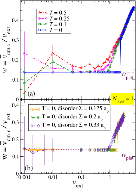
Figure 2(a) reports the time-averaged horizontal velocity of the single-layer lubricant CM, as a function of the velocity of a fully commensurate top layer () for several temperatures set by the Langevin thermostat. The velocity ratio is generally a nontrivial function of , that for low temperature (here and ) displays a wide flat plateau followed by a regime of continuous evolution. The plateau extends over a wide range of external driving velocities, up to a critical depinning velocity , whose precise value is obtained by ramping “adiabatically”. Beyond , the lubricant leaves the plateau speed and, at finite temperature, moves up toward the symmetrical speed , as dictated by the thermostat dissipation. At zero temperature, the plateau state is abandoned with a discontinuous jump of . The small- side of the plateau is difficult to address by numerical simulations, since the relative uncertainty in the determination of increases due to -independent thermal fluctuations of . By running longer averaging simulations at low , we mitigate the error bars over , and the data are consistent with a plateau dynamics extending all the way down to the static limit , like in the 1D model.Manini07PRE In particular, within the plateau, the calculation shows perfect matching of the mean lubricant velocity to the geometric ratio of Eq. (12). By increasing the temperature, deviates more and more from the perfect plateau value. At the highest temperature considered, , near melting of the LJ crystal at ,Ranganathan92 and even at the smaller no strict plateau is observed in the simulations. Note however that for the plateau attractor tends to affect the dynamics even in the presence of large thermal fluctuations. We have checked that finite-size scaling shows essentially no size effect on the plateau, and in particular on its boundary edge .
The dynamical pinning mechanism of the present 2D model is similar to that discussed for the simpler 1D model.Vanossi06 ; Manini07PRE The bottom layer produces a corrugated potential energy which, with its near-matching periodicity, is responsible for the creation of kinks, generally consisting of weak local compressions of the lubricant chain, with two lubricant atoms trapped in the attractive region between two bottom-substrate atoms. In the quantized-velocity state, these kinks become pinned to the upper slider (whose potential varies slowly on the lubricant interparticle scale) and are therefore dragged along.
We probe the robustness of the quantized plateau state even in the presence of an “irregular” (i.e., quenched-disordered) bottom substrate, by running simulations with its atoms randomly displaced, horizontally and vertically, away from the regular positions, Eq. (5), by a significant fraction of the lattice equilibrium spacing . Calculations still display the perfect plateau velocity, which however terminates at a lower . Figure 2b shows the results of one specific realization of the quenched disorder of 3 different amplitudes . By averaging over different realizations of disorder with the same amplitude , we obtain, for example, , compared to the value obtained for the case a perfectly crystalline bottom wall at .
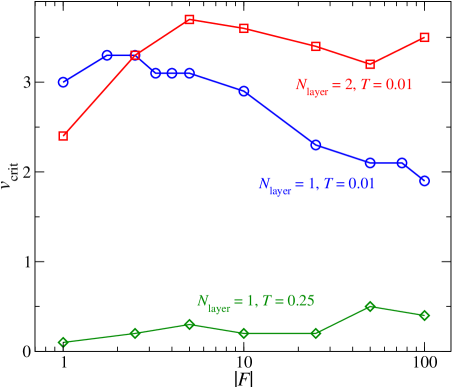
Our overall evidence is that, in the 2D system as much as in the more idealized 1D model, the phenomenon of velocity quantization is stable, reproducible and ubiquitous, and not the result of some careful tuning of parameters. In particular, Fig. 3 shows that the depinning velocity marking the end of the quantized plateau is a smooth function of the load applied to the top layer over two orders of magnitude. Calculations suggest that a moderate load near unity is beneficial to the quantized sliding, at least at the low temperature . This is the result of a competition between the beneficial role of load that limits thermally induced “slips” of the kinks, and the detrimental effect of limiting the vertical lubricant movements at high loads. Indeed, at higher temperature, where thermal fluctuations are more active in destabilizing the quantized state (thus yielding a smaller ), calculations show a general slow increase of with , favored by the suppression of thermally induced “slips” promoted by the stronger load-induced confinement.
Figure 3 shows that in the large-load low-temperature regime, the critical velocity for is even larger than for . In this plateau regime, we identify “horizontal” kinks in the lubricant layer adjacent to the bottom potential, while the upper lubricant layer shows weaker -spacing modulations.
IV Soliton coverage and lubricant softness
The perfect matching of the number of kinks to the number of top-atoms , as considered in all previous figures, is an especially favorable circumstance for kink dragging, thus for the quantized-plateau phenomenon, but not one to be expected to occur easily in actual lubricated sliding. It is therefore important to examine situations where this kind of full commensuration is absent.

In the following we study the behavior of the depinning point as a function of the commensuration ratio . In particular we keep fixed (i.e. the density of solitons), and vary the number of surface atoms in the top substrate. In Fig. 4 the depinning velocity , evaluated by adiabatically increasing of , is reported as a function of the commensuration ratio . While the dependence on kink coverage is rather erratic, we can recognize that tends to peak at or near integer values of . In contrast, a fractional displaced from commensurate regimes produces a weakening or even the loss of the quantized plateau, represented by . Figure 4 shows that this drop in is especially sharp for , for which many incommensurate coverages show no quantized plateau, even at the smallest accessible within practical simulation times. We conclude that the occurrence of quantized lubricant velocity plateaus, although comparably robust and widespread, may not be trivial to observe in practice: strongly incommensurate coverages and/or thick lubricant films could prevent its manifestation.
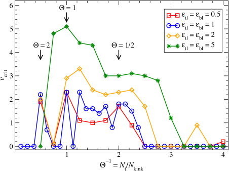
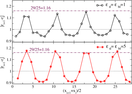
The detailed dependence of the depinning transition on coverage is affected by the relative “softness” of the lubricant. Figure 5 shows that when the interaction energy of the lubricant with the substrates is increased to become larger than the intra-lubricant interaction , as is the case for a soft lubricant wetting strongly the sliding surfaces, the quantized-plateau region extends generally to larger and to a wider range of coverages . The reason for this is illustrated by the configuration snapshots of Fig. 6: a comparably stronger interaction with the substrates favors the commensurate in-register lubricant regions, shrinking the kink size. Localized kinks are more suitable to being picked up and dragged by the corrugations of the top substrate.
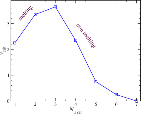
Figure 7 shows how the lubricant thickness affects the dynamically pinned state, i.e. as a function of the number of lubricant layers in the fully commensurate condition. The data show quantized-velocity plateaus, displaying a maximum extension for , followed by a decaying as the lubricant thickness increases beyond that value. For layers we could detect no velocity plateau, at least within the range accessible to a practical numerical integration of the equations of motion. Vertical corrugations of the lubricant induced by the kinks originating and propagating from the bottom substrate have the effect of mediating the kink tendency to pin to the top-layer corrugations, therefore favoring the observed perfect velocity quantization. For increasing , these -displacements decay rapidly, and this mechanism becomes less effective to support the dynamically pinned state.
Our calculations show that while the quantized plateau occurs when the solitons – misfit dislocations – are driven gently through the solid lubricant, the speed-induced transition to the dynamically unpinned state can involve the melting of the lubricant, due to the large Joule heating induced by shearing. By analyzing the detail of the depinning transition for , we observe two different depinning behaviors to the left and to the right, respectively, of the maximum shown in Fig. 7. For , the depinning transition changes the solid lubricant film into a disordered diffusive liquid, with a lower density, (thus characterized by an increase in ). By contrast, a lubricant composed of four or more layers remains essentially solid through the depinning transition. This is the case because the Joule heating produced by shearing is removed with sufficient efficiency by the thermostat so that the effective lubricant temperature remains moderate. The lubricant remains solid in particular when is small, as is the case for thick lubricant layers, but also for , or if a larger damping is introduced in the Langevin dynamics. This indicates that the quantitative details of the findings of the present section depend on the assumed dissipation mechanism, and could therefore vary between one or another specific experimental situation. Nonetheless the qualitative result that under suitable conditions the depinning could be associated to lubricant melting while under other conditions the lubricant could remain solid through the transition is expected to be real, and should be verifiable in real boundary-friction experiments.
V Friction
The (-directed) kinetic friction force that must be applied to the top slider to maintain its sliding motion balances instantaneously the force that the lubricant exerts on the top substrate. can be decomposed in several terms by analyzing the mechanical work done by the individual force contributions. The forces that the sliding top exerts on the lubricant [first term in Eq. (II)] produce a total work whose mean contribution to dissipation can be computed by evaluating the change in lubricant kinetic energy over a time interval
The first term in Eq. (V) represents precisely the contribution of the LJ top-lubricant interactions to , plus bounded terms which do fluctuate, contributing a limited [order ] potential-energy change in the limit of a long time integration. The second term is proportional to the kinetic energy averaged over the time interval. The last term in (V) describes the correlation of the random forces and the lubricant velocities. By careful integration over the trajectory produced by the Langevin dynamics, averaging over the distribution of the random variables (indicated by angular brackets), and recalling Eq. (9), this term is evaluated as
| (15) | |||
| (16) | |||
| (17) | |||
| (18) |
The factor 2 in line (17) comes from summing and components, and the factor in the integral of line (18) is the result of integrating the Dirac delta at the integration boundary. We observe that, like the conservative potential energy terms, the lubricant kinetic energy deviation is of order over a long time integration. By combining Eq. (V) with the result of Eq. (18), in this large- limit the average dissipated work becomes
| (20) | |||||
The fourth and last term in square brackets is added to account for the work done by the top substrate directly against the dissipation forces of Eq. (11). We omit the explicit indication of the averaging over the Langevin noise, which becomes irrelevant in the limit of a long averaging time .
This total dissipated energy is conveniently written in a form where we measure the particles velocities relative to the instantaneous center-mass velocity . Indeed, by using and omitting corrections of order , we can rewrite the dissipated energy as
where terms linear in vanish due to the definition of , and is the kinetic energy in the instantaneous CM frame:
| (22) |
The work that the top layer does on the lubricant is supplied by the kinetic friction force [the top-substrate vertical motion only yields a work of order ], and equals . This relation provides an instructive decomposition of the average kinetic friction force:
Equation (V) expresses the kinetic friction force as the sum of two contributions. The first and most important term is the contribution of the fluctuations of the lubricant-particle velocities in the instantaneous CM frame, reduced by the thermostat-set value. Even at , this term would vanish in the event that the lubricant moved as a rigid whole. The term in the final line can be interpreted as the friction force that dissipative phenomena with the bottom and the top respectively would produce, again even if the lubricant was rigid. This trivial term related to the overall CM motion yields a minimum total friction force whenever , which corresponds to for the main horizontal component. In fact, this trivial contribution originates the tendency of to abandon the plateau and reach 0.5, as in Figs. 2, and 8, 9 in the large sliding speed limit where this trivial term dominates. Equation (V) can be reformulated in terms of an effective temperature of the steady state:
The formulation (V), clarifies the contribution of friction to Joule heating, and shows explicitly the irrelevant role of the trivial dissipation terms in this respect.
Our MD simulations allow us to calculate instantaneously the (-directed) kinetic friction by considering the longitudinal force component that the lubricant exerts on the top driven substrate. By time averaging, the value obtained coincides precisely with that evaluated through Eq. (V).
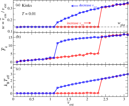
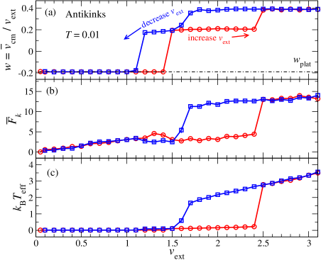
A direct numerical evaluation of the friction force is shown in panels (b) of Figs. 8 and 9 for the kink and the anti-kink geometries, respectively, depicting typical scans where is cycled adiabatically up and down in small steps. Like in the simulations of the 1D sliding model,Manini07PRE ; Vanossi07Hyst ; Vanossi07PRL and as is well known for the static pinning/depinning of the standard FK model,Braun97 ; Vanossi04 ; VanossiJPCM the present 2D model displays a clear hysteretic behavior of the velocity-plateau state (panels (a)), provided that thermal fluctuations are much smaller than the energy barrier hindering the full exploration of phase space for any affordable simulation time. A clear correlation of with the effective lubricant temperature (panels Fig. 8c and 9c) is evident, but the trivial contribution is also seen to play a quantitative role. The bistability region with a clear hysteretic loop allows us to gauge the tribological effect of the quantized plateau state. In the kink geometry, Fig. 8 makes it apparent that friction is significantly less in the pinned quantized state than in the depinned state, all other parameters being equal. Figure 9 shows a similar tribological behavior, but with the occurrence of an additional intermediate approximately quantized velocity plateau (the 1D model displayed similar intermediate plateaus Vanossi06 ). The difference in friction between the primary and the secondary plateaus is a small one, with slightly less friction in the latter state. Comparison of the curves in panels 9b and 9c demonstrates that this effect is entirely due to the trivial friction term. This term is very large in the primary plateau because of the great difference of from the optimal symmetrical drift ; in passing to the secondary plateau, the trivial friction term decreases quite substantially, but the kinetic fluctuation contribution to friction increases by a similar amount.
VI Intermittent dynamics at the plateau state
So far, we assumed some fixed externally imposed speed for the top slider. In a standard tribological simulation, the slider is instead generally pulled through a spring of given stiffness whose other end is moved at constant velocity.VanossiJPCM The spring can be viewed as a way to mimic not only the experimental driving device, but also the elasticity of the sliding substrates. From an experimental point of view, frictional forces may display a typical sawtooth dependence at sufficiently low driving external velocities, the hallmark of the intermittent stick-slip dynamics. The details of this low-driving behavior of course depend sensitively on the mechanical properties of the device that applies the stress.

Beside constant speed, we also explored the model with the spring pulling method. We obtained the quantized sliding state, also with the spring, and the simulations showed differences with the constant-speed method only in the fine detail. For this reason we omit here to display and analyze those results in detail.
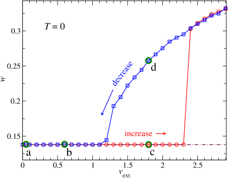
In fact, even within the rigid-drive model, for sufficiently low sliding speed and for extremely small thermal fluctuations (i.e., ), we did observe a stick-slip intermittent dynamical regime in the total force applied to the sliding top substrate in order to keep its sliding speed constant. Figure 10 depicts a typical adiabatic up-down scan of , similar to Fig. 8a but at . To get insight into the different dynamical regimes outside and inside the bistability region, Fig. 11 analyzes in detail the four points marked in Fig. 10, three of which belong to the plateau state and one outside of it. Each of the four panels of Fig. 11 compares the time evolution of the lubricant CM velocity to the corresponding instantaneous kinetic friction force .
For the first two plateau points (a) and (b) at low , the typical sawtooth time dependency of is clearly visible. In these regimes of motion, the rescaled lubricant CM velocity performs tiny periodic oscillations around the quantized plateau value and exhibits an intermittent, almost regular, stick-slip pattern. This oscillatory phenomenology is understood as the kink array being dragged at full velocity across the associated periodic Peierls-Nabarro potential.Braunbook Indeed, the oscillation frequency matches the washboard frequency of the kinks multiplied by their number in these simulations, due to the four equally-spaced kinks crossing sequentially the corresponding Peierls-Nabarro barriers. A much less regular pattern would arise in a geometry. Due to the rather extended nature of solitons and smaller amplitude of the Peierls-Nabarro barrier with respect to the full atomic corrugation, the quantized plateau stick-slip regime is associated to much lower dissipation than regular stick-slip dynamics as seen in dry friction AFM experiments.Verhoeven04 ; Maier08 By further increasing the external driving speed to , panel (c), the kinetic friction becomes a little more “erratic”, with an extra modulation of the sawtooth shape, resembling a sort of inverted stick-slip. Panel (d) displays the dynamics for the same , but obtained while cycling down: this depinned state shows large fluctuations both in and , giving rise to significant tribological dissipation, as expressed by the first term of Eq. (V).
VII Discussion and conclusions
The present simulation work is meant to characterize tribologically the quantized sliding state discovered in a 1D sliding model Vanossi06 and later observed in a substantially less idealized 2D model.Castelli08Lyon The perfectly quantized plateau is demonstrated here to extend over broad parameter ranges of the model, being robust against the effects of thermal fluctuations, quenched disorder in the confining substrates, the presence of confined multiple (up to 6) lubricant layers, and over a wide interval of loading forces. When temperature becomes comparable to the lubricant melting point, the plateau state tends to deteriorate and eventually disappears, but the geometrically determined velocity ratio , acting as an attractor, leaves anyway a trace in the ensuing “noisy” dynamics.
The velocity plateau, as a function of , ends at a critical velocity , and for the lubricant tends to accelerate toward a speed . This result, dictated by the symmetric choice of the Langevin thermostat dissipation, may change in real systems where heat dissipation occurs through generally asymmetric sliders.
Our calculations show that while the quantized plateau occurs when the solitons are driven gently through the solid lubricant, the speed-induced transition at can involve the melting of the lubricant, due to the large Joule heating induced by large velocity shearing.The depinning value is linked to the rate of commensuration of kinks to the upper slider periodicity: a particularly robust plateau signaled by a local maximum of is located at well-commensurate values, especially . Besides, the lubricant softness, setting the width of the propagating solitonic structures, is found to play a major role in promoting in-registry contact regions beneficial to this quantized sliding. Our typical dynamical depinning speed , is of the order of a few model units (corresponding to sliding speed values ranging from tens to thousands m/s for realistic choices of model parameters), is very large compared to typical sliding velocities investigated in experiments. This suggests that in practice sliding at a dynamically quantized velocity is likely to be extremely robust. In real experimental systems, deterioration of the quantized sliding state will most probably associated to mechanisms such as disorder, boundary effects, or unfavorable lubricant-substrate incommensurate geometries, rather than to excessive driving speed.
By cycling in underdamped regime, the layer sliding velocity exhibits a hysteretic loop around , like in the 1D model.Vanossi07PRL The bistability region allows us to gauge the tribological effect of the quantized plateau state. So, in the framework of Langevin dynamics, by evaluating the force instantaneously exerted on the top plate, we find that this quantized sliding represents a dynamical “pinned” state, characterized by significantly low values of the kinetic friction. A characteristic backward lubricant motion produced by the presence of “anti-kinks”, has also been observed in this context. This peculiar backward motion is likely to represent the most curious evidence of the quantized plateau state when – as we hope – it will be investigated experimentally.
On the theoretical side, the role of substrate deformability and defects in the lubricant structure, together with a realistic three dimensional description, with force fields representative of a concrete lubricated configurations, will certainly require further investigations.
Acknowledgments
This work was supported by CNR, as a part of the European Science Foundation EUROCORES Programme FANAS. R.C. and A.V. acknowledge gratefully the financial support by the Regional Laboratory InterMech - NetLab “Surfaces & Coatings for Advanced Mechanics and Nanomechanics” (SUP&RMAN), and of the European Commissions NEST Pathfinder program TRIGS under Contract No. NEST-2005–PATHCOM-043386.
References
- (1) J. Gao, W. D. Luedtke, and U. Landman, J. Chem. Phys. 106, 4309 (1997).
- (2) U. Tartaglino, I. M. Sivebaek, B. N. J. Persson, and E. Tosatti, J. Chem. Phys. 125, 014704 (2006).
- (3) J. Klein and E. Kumacheva, J. Chem. Phys. 108, 6996 (1998).
- (4) G. He, M. H. Müser, Mark O. Robbins, Science 284, 1650 (1999).
- (5) A. Vanossi, N. Manini, G. Divitini, G. E. Santoro, and E. Tosatti, Phys. Rev. Lett. 97, 056101 (2006).
- (6) N. Manini, M. Cesaratto, G. E. Santoro, E. Tosatti, and A. Vanossi, J. Phys.: Condens. Matter 19, 305016 (2007).
- (7) A. Vanossi, N. Manini, F. Caruso, G. E. Santoro, and E. Tosatti, Phys. Rev. Lett. 99, 206101 (2007).
- (8) N. Manini, A. Vanossi, G. E. Santoro, and E. Tosatti, Phys. Rev. E 76, 046603 (2007).
- (9) N. Manini, G. E. Santoro, E. Tosatti, and A. Vanossi, J. Phys.: Condens. Matter 20, 224020 (2008).
- (10) G. E. Santoro, A. Vanossi, N. Manini, G. Divitini, and E. Tosatti, Surf. Sci. 600, 2726 (2006).
- (11) M. Cesaratto, N. Manini, A. Vanossi, E. Tosatti, and G. E. Santoro, Surf. Sci. 601, 3682 (2007).
- (12) A. Vanossi, G. E. Santoro, N. Manini, M. Cesaratto, and E. Tosatti, Surf. Sci. 601, 3670 (2007).
- (13) A. Vanossi, G. E. Santoro, N. Manini, E. Tosatti, and O. M. Braun, Tribol. Int. 41, 920 (2008).
- (14) O. M. Braun, A. Vanossi, and E. Tosatti, Phys. Rev. Lett. 95, 026102 (2005).
- (15) I. E. Castelli, N. Manini, R. Capozza, A. Vanossi, G. E. Santoro, and E. Tosatti, J. Phys.: Condens. Matter 20, 354005 (2008).
- (16) D. Frenkel and B. Smit, Understanding Molecular Simulation. From Algorithms to Applications (Academic Press, London, 1996).
- (17) G. J. Martyna, M. L. Klein and M. Tuckerman, J. Chem. Phys. 97, 2635 (1992).
- (18) C. W. Gardiner, Handbook of Stochastic Methods for Physics, Chemistry and the Natural Sciences (Springer-Verlag, Berlin, 1985).
- (19) W. H. Press, S. A. Teukolsky, W. T. Vetterling and B. P. Flannery, Numerical Recipes in Fortran. The Art of Parallel Scientific Computing (Cambridge University Press, Cambridge, 1996).
- (20) S. Ranganathan and K. N. Pathak, Phys. Rev. A 45, 5789 (1992).
- (21) O. M. Braun, A. R. Bishop, and J. Röder, Phys. Rev. Lett. 79, 3692 (1997).
- (22) A. Vanossi, G. Santoro, and V. Bortolani, J. Phys.: Condens. Matter 16, S2895 (2004).
- (23) A. Vanossi and O. M. Braun, J. Phys.: Condens. Matter 19, 305017 (2007).
- (24) O. M. Braun and Yu. S. Kivshar, The Frenkel-Kontorova Model: Concepts, Methods, and Applications (Springer-Verlag, Berlin, 2004).
- (25) G. S. Verhoeven, M. Dienwiebel, and J. W. M. Frenken, Phys. Rev. B 70, 165418 (2004).
- (26) S. Maier, E. Gnecco, A. Baratoff, R. Bennewitz, and E. Meyer, Phys. Rev. B 78, 045432 (2008).