Cosmological constraints on DGP braneworld gravity with brane tension

Abstract

We perform a Markov chain Monte Carlo analysis of the self-accelerating and normal branch of Dvali-Gabadadze-Porrati braneworld gravity. By adopting a parametrized post-Friedmann description of gravity, we utilize all of the cosmic microwave background data, including the largest scales, and its correlation with galaxies in addition to the geometrical constraints from supernovae distances and the Hubble constant. We find that on both branches brane tension or a cosmological constant is required at high significance with no evidence for the unique Dvali-Gabadadze-Porrati modifications. The crossover scale must therefore be substantially greater than the Hubble scale $H_{0}r_{c}>3$ and 3.5 at the 95% C.L. with and without uncertainties from spatial curvature. With spatial curvature, the limit from the normal branch is substantially assisted by the galaxy cross correlation which highlights its importance in constraining infrared modifications to gravity.

I Introduction

Cosmological tests of the acceleration of the expansion offer unique opportunities to test gravity on large scales and low curvature. Dvali, Gabadadze, and Porrati (DGP) dvali:00 proposed that such infrared modifications to gravity might arise in a braneworld model where our Universe is a 4D brane embedded in a 5D bulk.

The two branches of cosmological solutions in the DGP model have distinct properties. In the so-called self-accelerating branch, late-time acceleration of the Universe occurs without the need of a cosmological constant deffayet:01 . Unfortunately without a cosmological constant, the self-accelerating branch predicts cosmological observables that are now in substantial conflict with the data (e.g. fairbairn:06 ; maartens:06 ; fang:08 ). Moreover, the linearized theory implies the presence of ghost degrees of freedom (e.g. luty:03 ; charmousis:06 ). The former problem can be alleviated with the restoration of a cosmological constant or brane tension. A definitive assessment of the latter problem awaits nonlinear solutions dvali:06 ; koyama:07 . On the second or normal branch, self-acceleration does not occur but interestingly phantom effective equations of state with $p/\rho<-1$ can be achieved without ghosts with the help of brane tension sahni:02 . In both cases, brane tension is required but substantial modifications to large-scale gravitational dynamics can still persist.

In this paper, we conduct a Markov chain Monte Carlo (MCMC) study of both branches of the DGP model using data from cosmic microwave background (CMB) anisotropies, supernovae distances, and the Hubble constant. For observables in the linear regime, we adopt the parametrized post-Friedmann (PPF) framework hu:07 ; hu:08 and its implementation into a standard Einstein-Boltzmann linear theory solver fang:08 ; fang:08b for the theoretical predictions. This framework allows us to include information from the near horizon scales which are crucial for assessing the viability of the self-accelerating branch. We also utilize information from the cross correlation between high-redshift galaxies and the CMB which has been proposed as an interesting test of both the self-accelerating and normal branches song:06 ; song:07 ; giannantonio:08 .

In Sec. II, we review the theory of the normal and self-accelerating branches of DGP gravity and their approximation through the PPF formalism. We present the results of our MCMC study in Sec. III and discuss them in Sec. IV. Finally, the details about the modifications to the ISWWLL code ho:08 ; hirata:08 used for the galaxy-ISW cross-correlation observations are specified in the Appendix.

II Normal and Self-accelerating Branches

In the DGP model dvali:00 our Universe is a (3+1)-brane embedded in a 5D Minkowski space described by the action

$$S = -\frac{1}{2\kappa^{2}}\int d^{5}x\sqrt{-\hat{g}}\hat{R}-\frac{1}{2\mu^{2}}\int d^{4}x\sqrt{-\tilde{g}}\tilde{R}$$ (1)

$$+\int d^{4}x\sqrt{-\tilde{g}}L_{T},$$

where 5D quantities are denoted by hats and 4D quantities are denoted by tildes. Matter fields, including a cosmological constant or brane tension and represented by $L_{T}$, are confined to the brane while only gravity extends to the full 5D bulk. We assume that there is no bulk tension. The constants $\kappa^{2}$ and $\mu^{2}$ are proportional to the inverse Planck masses in the bulk and brane, respectively.

Gravity on the brane is consequently modified at large scales. In particular, the crossover distance $r_{c}=\kappa^{2}/2\mu^{2}$ governs the transition from 5D to 4D scalar-tensor gravity. On scales smaller than the Vainshtein radius $r_{*}=(r_{c}^{2}r_{g})^{1/3}$, nonlinear interactions return gravity to general relativity around a point mass with Schwarzschild radius $r_{g}$. In the following sections we describe the evolution of the background and linear density perturbations in the two branches of cosmological solutions.

II.1 Background expansion

Variation of the action yields the modified Einstein equations on the brane which reduce to the modified Friedmann equation in a homogeneous and isotropic metric

$$H^{2}-\frac{\sigma}{r_{c}}\sqrt{H^{2}+\frac{K}{a^{2}}}=\frac{\mu^{2}}{3}\sum_{i}\rho_{i}-\frac{K}{a^{2}},$$ (2)

where $H=\dot{a}/a$ is the Hubble parameter, $K$ is the spatial curvature, $a$ is the scale factor, and $\rho_{i}$ are the energy densities of the various components on the brane. Here $\sigma=\pm 1$ and designates the branch of the cosmological solutions.

For $\sigma=+1$, late-time acceleration occurs even without a cosmological constant $\Lambda$ deffayet:01 and so this branch is referred to as self-accelerating DGP (sDGP). In order to separate tests of gravity from explanations of acceleration, we will also study the sDGP branch supplemented by a nonvanishing $\rho_{\Lambda}$ which we denote as sDGP+$\Lambda$ where confusion might arise. For $\sigma=-1$, DGP modifications slow the expansion rate and the branch is referred to as normal DGP (nDGP). Here, a cosmological constant is required in order to achieve late-time acceleration.

With the usual definitions $\Omega_{i}=\mu^{2}\rho_{i}(a=1)/H_{0}^{2}$ and $\Omega_{K}=-K/H_{0}^{2}$, the modified Friedmann equation becomes

$$\left(\frac{H}{H_{0}}\right)^{2} = \left(\sqrt{\frac{\Omega_{m}}{a^{3}}+\frac{\Omega_{r}}{a^{4}}+\Omega_{\Lambda}+\Omega_{r_{c}}}+\sigma\sqrt{\Omega_{r_{c}}}\right)^{2}$$ (3)

$$+\frac{\Omega_{K}}{a^{2}},$$

where we have assumed that the energy density components include nonrelativistic matter, radiation, and possibly a cosmological constant. Here

$$\sqrt{\Omega_{r_{c}}}\equiv\frac{1}{2H_{0}r_{c}}=\sigma\frac{\Omega_{\rm DGP}}{2\sqrt{1-\Omega_{K}}},$$ (4)

where

$$\Omega_{\rm DGP} = 1-\Omega_{m}-\Omega_{r}-\Omega_{\Lambda}-\Omega_{K}$$ (5)

represents the effective contribution of the DGP modification to the energy density assuming the ordinary Friedmann equation. Specifically,

$$\rho_{\rm DGP}\equiv\frac{3}{\mu^{2}}\left(H^{2}+\frac{K}{a^{2}}\right)-\sum_{i}\rho_{i}.$$ (6)

As with any real energy density component, it obeys the conservation equation

$$\rho_{\rm DGP}^{\prime}=-3(1+w_{\rm DGP})\rho_{\rm DGP}.$$ (7)

Using Eqs. (2) and (7), we derive

$$1+w_{\rm DGP}=\frac{\frac{\mu^{2}}{3}\sum_{i}(1+w_{i})\rho_{i}}{H^{2}+\frac{K}{a^{2}}+\frac{\mu^{2}}{3}\sum_{i}\rho_{i}}.$$ (8)

For cases with a cosmological constant it is also useful to define the total effective dark energy

$$\rho_{e}=\rho_{\rm DGP}+\rho_{\Lambda}$$ (9)

and its equation of state

$$1+w_{e}=(1+w_{\rm DGP})\frac{\rho_{\rm DGP}}{\rho_{\rm DGP}+\rho_{\Lambda}}\,.$$ (10)

In nDGP this quantity diverges when the DGP and $\Lambda$ density terms are equal and opposite at which point the value of $1+w_{e}$ switches sign. In particular, its value today is given by

$$w_{0}=-\frac{1-\Omega_{K}}{1-\Omega_{K}-\Omega_{m}}\frac{1-\Omega_{K}-\Omega_{m}+\Omega_{\Lambda}}{1-\Omega_{K}+\Omega_{m}+\Omega_{\Lambda}},$$ (11)

where we have neglected the small radiation contribution. With realistic cosmological parameters $w_{0}>-1$ and $w_{0}<-1$ for sDGP and nDGP, respectively, with $w_{0}=-1$ being the limit of cosmological constant domination in either case.

II.2 PPF linear theory

Unlike the background, the evolution of density and metric perturbations on the brane require solutions for the bulk metric equations. The parametrized post-Friedmann framework was introduced in Refs. hu:07 ; hu:08 to encapsulate these effects in an effective 3+1 description. Fits to the bulk calculation in sDGP without $\Lambda$ or curvature from sawicki:06 were given in hu:07 and incorporated into the linear theory code CAMB lewis:00 in fang:08 . We extrapolate these fits to cases with $\Lambda$ and curvature here though we caution the reader that these have not been tested by explicit bulk calculations. For nDGP, we utilize a description from seahra:09 based on bulk calculations from song:07 and cardoso:08 with $\Lambda$ but no curvature. We again extrapolate these results for spatial curvature. The errors induced by these extrapolations are controlled given the well-defined limits of $\Lambda$ domination and the small dynamical effects of curvature in the regime we consider.

Given the expansion history, the PPF framework is defined by three functions and one parameter. From these quantities, the dynamics are determined by conservation of energy and momentum and the Bianchi identities. The defining quantities are $g(a,k)$ which quantifies the effective anisotropic stress of the modifications and distinguishes the two gravitational potentials, $f_{\zeta}(a)$, which defines the relationship between the matter and the metric on superhorizon scales, and $f_{G}(a)$, which defines it in the linearized Newtonian regime. The additional parameter defines the transition scale between the superhorizon and Newtonian behaviors.

More specifically,

$$g(a,k)\equiv\frac{\Phi+\Psi}{\Phi-\Psi},$$ (12)

where the scalar linear perturbations are represented in longitudinal gauge

$$ds^{2}=-(1+2\Psi)dt^{2}+a^{2}(1+2\Phi)dx^{2},$$ (13)

where $dx^{2}$ is the unperturbed spatial line element with constant curvature $K$. In the quasistatic high $k$ limit, the DGP model predicts

$$g_{\rm QS}=-\frac{1}{3}\left[1-\frac{2\sigma Hr_{c}}{\sqrt{1-\Omega_{K}(a)}}\left(1+\frac{H^{\prime}}{3H}-\frac{2}{3}\Omega_{K}(a)\right)\right]^{-1},$$ (14)

where $\Omega_{K}(a)=H_{0}^{2}\Omega_{K}/H^{2}a^{2}$. On superhorizon scales, we take for sDGP hu:07

$$g_{\rm SH,sDGP}(a) = \frac{9}{8Hr_{c}\sqrt{1-\Omega_{K}(a)}-1}$$

$$\times\left(1+\frac{0.51}{Hr_{c}\sqrt{1-\Omega_{K}(a)}-1.08}\right).$$

We exclude models $\sqrt{1-\Omega_{K}}H_{0}r_{c}>1.08$ from consideration as they are not within the domain of applicability of the fit nor are they cosmologically viable. For nDGP we take seahra:09 (cf. afshordi:08 )

$$g_{\rm SH,nDGP}(a)=-\frac{1}{2Hr_{c}\sqrt{1-\Omega_{K}(a)}+1}.$$ (16)

The corrections for curvature have not been verified by a bulk calculation for the superhorizon cases. For the curvatures that we will consider the total impact is small as can be verified by omitting the correction. We expect therefore that corrections on the correction have negligible impact.

At intermediate scales, $g$ is fitted by the interpolating function

$$g(a,k)=\frac{g_{\rm SH}+g_{\rm QS}(c_{g}k_{H})^{n_{g}}}{1+(c_{g}k_{H})^{n_{g}}},$$ (17)

where $k_{H}=k/aH$, $c_{g}=0.14$ for sDGP and $c_{g}=0.4$ for nDGP, respectively. Furthermore, we set $n_{g}=3$.

The function $f_{\zeta}(\ln a)$ relates the metric to the density at superhorizon scales and is well described by $f_{\zeta}(\ln a)=0.4g_{\rm SH}(\ln a)$. In the quasistatic regime, the analogous relationship between $\Phi-\Psi$ and the density is the Poisson equation and that is unmodified from ordinary gravity for DGP. Hence $f_{G}(\ln a)=0$.

Finally the parameter $c_{\Gamma}$ relates the transition scale in the dynamical equations from superhorizon to quasistatic behavior. For sDGP we take $c_{\Gamma}=1$ following hu:07 and we employ this value for cases that include $\Lambda$. In nDGP, $c_{\Gamma}\sim 0.15$ from seahra:09 implying a delayed approach to quasistatic behavior.

III Constraints on the Models

We will use a variety of cosmological data sets to constrain the two branches of the DGP models. First we use the CMB anisotropy data from the five-year Wilkinson Microwave Anisotropy Probe (WMAP) WMAP:08 , the Arcminute Cosmology Bolometer Array Receiver (ACBAR) ACBAR:07 , the Cosmic Background Imager (CBI) CBI:04 , and the Very Small Array (VSA) VSA:03 . Next we employ data from the Supernovae Legacy Survey (SNLS) SNLS:06 and the measurement of the Hubble constant from the Supernovae and $H_{0}$ for the Equation of State (SHOES) SHOES:09 program. Finally we take galaxy-ISW (gISW) correlation observations using the likelihood code of  ho:08 ; hirata:08 . We quote results with and without the gISW constraint to highlight its impact on the results.

In Sec. III.1 we discuss the predictions for these observables in the two branches of the DGP model. In Secs. III.2 and III.3 we present the results of a MCMC-likelihood analysis for flat and nonflat universes, respectively. The MCMC analysis is conducted with the publicly available CosmoMC lewis:02 package.

III.1 Model predictions

In this section we illustrate model predictions of the various cosmological observables we use in the constraints. We chose the parameters of the various models that highlight results from the MCMC analysis.

At high redshifts the DGP modifications become negligible on either branch [see Eq. (3)], and so we choose a parametrization that separates high-redshift and low-redshift constraints. Specifically we take 6 high-redshift parameters: the physical baryon and cold dark matter energy density $\Omega_{b}h^{2}$ and $\Omega_{c}h^{2}$, the ratio of sound horizon to angular diameter distance at recombination multiplied by a factor of 100 $\theta$, the optical depth to reionization $\tau$, the scalar tilt $n_{s}$, and amplitude $A_{s}$ at $k_{*}=0.002~{}\textrm{Mpc}^{-1}$.

The low-redshift parameters differ in the various classes of models. For flat $\Lambda$CDM and sDGP without $\Lambda$ there are no additional degrees of freedom. Note that $\theta$ carries information on $H_{0}$. For flat sDGP$+\Lambda$ and nDGP, $\Omega_{\Lambda}$ is an extra degree of freedom. For the open versions of all models $\Omega_{K}$ is the final degree of freedom.

For $\Lambda$CDM and sDGP we illustrate predictions from the nonflat maximum likelihood models found in the next section (see Tables 6 and 7). Since the large-scale behavior of nDGP is new to this work, we highlight the dependence of observables on $\Omega_{\Lambda}$ and $\Omega_{K}$ while keeping the high-redshift cosmological parameters fixed (see Table 1). Note in the $r_{c}\rightarrow 0$ limit where $\Omega_{r_{c}}=0$, both nDGP and sDGP+$\Lambda$ become $\Lambda$CDM. We therefore choose to illustrate the maximum likelihood sDGP model with $\Lambda=0$.

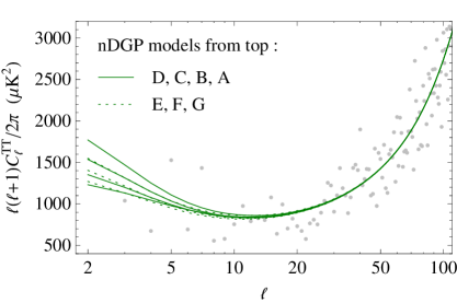
nDGP	A	B	C	D	E	F	G
$\Omega_{\Lambda}$	0.77	1.00	1.25	1.50	1.50	1.25	1.00
$\Omega_{K}$	–	–	–	–	-0.025	-0.015	-0.010
$\Omega_{r_{c}}$	0.000	0.012	0.049	0.114	0.132	0.057	0.015
$H_{0}$	73	77	82	86	71	72	71

Table 1: Different choices of nDGP models for illustration. Note that nDGP-A is the best-fit (with gISW) flat nDGP model, corresponding to $\Lambda$CDM. Other chain parameters are fixed to values in Table 5.

III.1.1 Cosmic microwave background

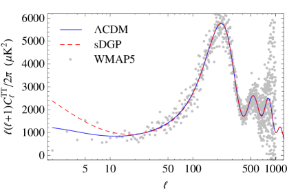
The CMB probes the geometry of the background expansion as well as the formation of large-scale structure. The latter manifests itself on the largest scales through the integrated Sachs-Wolfe (ISW) effect from the evolution of the gravitational potential. To predict these effects we implement the PPF modifications from Sec. II.2. The incorporation of the PPF formalism into a standard Einstein-Boltzmann linear theory solver yields an efficient way to obtain predictions of the DGP model for the CMB. We utilize the PPF modifications to CAMB lewis:00 implemented in Refs. fang:08 ; fang:08b , which we can apply directly for sDGP and figure as a starting point for the implementation of nDGP and sDGP+$\Lambda$. In Fig. 1, we plot the CMB temperature anisotropy power spectrum with respect to angular multipole $\ell$ for the best-fit models of $\Lambda$CDM and sDGP, as well as the nDGP parameter choices given in Table 1.

Relative to $\Lambda$CDM, the growth of structure is suppressed in the sDGP model, yielding an ISW enhancement at the lowest multipoles. This enhancement is sufficiently large to bring the sDGP model without $\Lambda$ into serious conflict with the joint data fang:08 . The opposite effects occurs in the nDGP model and lead to predictions that are compatible with CMB data. Here raising $\Omega_{\Lambda}$ at fixed $\Omega_{K}$ enhances the low multipoles through the ISW effect. However, compensating effects from curvature can lead to parameter degeneracies.

At high redshifts the contribution of $\Omega_{r_{c}}$ to the Hubble parameter, Eq. (3), becomes negligible in either branch. The CMB acoustic peaks can therefore be utilized as usual to infer constraints on the high-redshift parameters, in particular, the physical energy densities of baryonic matter and dark matter as well as the angular diameter distance to recombination.

Figure 1: Best-fit CMB temperature anisotropy power spectrum for $\Lambda$CDM and sDGP (left panel). Examples of nDGP models (right panel) illustrate the degeneracy between $\Omega_{\Lambda}$ and $\Omega_{K}$ corresponding to models in Table 1.

III.1.2 Distances to the supernovae and $H_{0}$

The comparison of the magnitudes of high-redshift to low-redshift supernovae yields a relative distance measure. Theoretical predictions for the distance modulus are related to the luminosity distance, $d_{L}(z)=(1+z)r(z)$, where $r(z)$ is the comoving angular diameter distance defined by

$$r(z)=\left\{\begin{array}[]{ll}\sin\left[H_{0}\sqrt{-\Omega_{K}}\chi(z)\right]/H_{0}\sqrt{|\Omega_{K}|},&\Omega_{K}<0,\\ \chi(z),&\Omega_{K}=0,\\ \sinh\left[H_{0}\sqrt{\Omega_{K}}\chi(z)\right]/H_{0}\sqrt{|\Omega_{K}|},&\Omega_{K}>0,\end{array}\right.$$ (18)

where the comoving radial distance $\chi$ is

$$\chi(z)=\int_{0}^{z}\frac{dz^{\prime}}{H(z^{\prime})}.$$ (19)

The supernovae magnitudes, once standardized, are related to the distance by

$$m\equiv\mu+M=5\log_{10}{d_{L}}+M+25,$$ (20)

where $d_{L}$ is in units of Mpc. The unknown absolute magnitude $M$ of the supernovae is a nuisance parameter in the fit and is degenerate with $H_{0}$. Hence supernovae measure relative distances within the set.

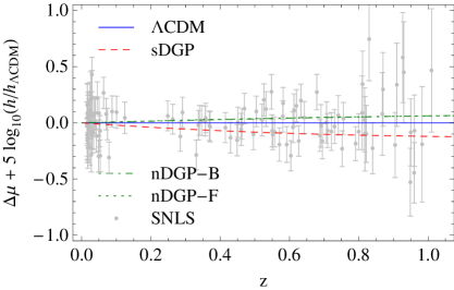
In Fig. 2, we plot the predictions for the distance modulus for the SNLS data in sDGP gravity, nDGP-B, nDGP-F, and in the $\Lambda$CDM model.

Figure 2: Best-fit distance modulus for sDGP, as well as the overlapping predictions for nDGP-B and nDGP-F with respect to $\Lambda$CDM.

The acoustic peaks in the CMB and the measurement of the local Hubble constant additionally provide absolute distance probes which complement the relative distance measure of the supernovae. For the Hubble constant, we take the SHOES measurement of $H_{0}=74.2\pm 3.6$ km s^-1 Mpc^-1 which employs Cepheid measurements to link the low-redshift supernovae to the distance scale established by the maser galaxy NGC 4258.

III.1.3 Galaxy-ISW cross correlations

The correlation between galaxy number densities and the CMB anisotropies can be used to isolate the ISW effect in the CMB. The enhanced ISW effect exhibited in the sDGP model without $\Lambda$ leaves a strong imprint on the large scales of the CMB temperature anisotropy. As pointed out by Song et al. song:06 , an interesting consequence of this is a considerable correlation of high-redshift galaxies with the CMB.

For nDGP gravity, whereas the ISW effect does not exhibit a substantial impact on the largest scales in the CMB, useful signatures remain in the correlations with galaxies that can break parameter degeneracies giannantonio:08 .

We evaluate the gISW cross correlations in the Limber and quasistatic approximation, as it is done in the ISWWLL code ho:08 ; hirata:08 used for the data analysis. Therefore, we write

$$C_{\ell}^{g_{j}T} \simeq \frac{3\Omega_{m}H_{0}^{2}T_{\rm CMB}}{(\ell+1/2)^{2}}\int dz\>f_{j}(z)H(z)D(z)$$ (21)

$$\times\frac{d}{dz}[D(z)(1+z)]P\left(\frac{\ell+1/2}{\chi(z)}\right).$$

Here, $D(z)$ is the linear growth rate in the quasistatic regime defined by $\Delta_{m}(k,z)=\Delta_{m}(k,0)D(z)/D(0)$, where $\Delta_{m}(k,z)$ is the matter density perturbation. $P(k)$ is the matter power spectrum today.

The approximations in Eq. (21) become accurate at the percent level for $\ell\gtrsim 10$. This condition is satisfied by about 90% of the total 42 data points that are used in the ISWWLL code. We discuss details about the approximations and the data in the Appendix. The data are divided into nine galaxy sample bins $j$, i.e., 2MASS0-3, LRG0-1, QSO0-1, and NVSS. The function $f_{j}(z)$ relates the matter density to the observed projected galaxy overdensity with $f_{j}(z)=b_{j}(z)\Pi_{j}(z)$ in the absence of magnification bias. $\Pi_{j}(z)$ is the redshift distribution of the galaxies and the bias factor $b_{j}(z)$ is assumed independent of scale, but dependent on redshift. The code determines $f_{j}(z)$, among other things, from fitting autopower spectra and cross-power spectra between the samples.

Figure 3: Best-fit $\Lambda$CDM and sDGP galaxy-ISW cross correlations for the different galaxy samples, roughly ordered in increasing effective, bias-weighted, redshift. Note the distinct predictions for the previously degenerate nDGP-B and nDGP-F models.

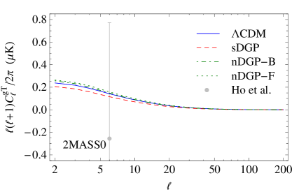
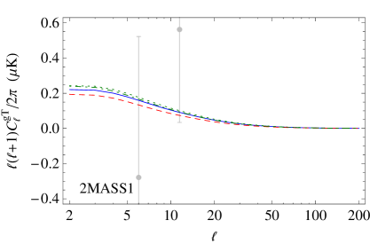
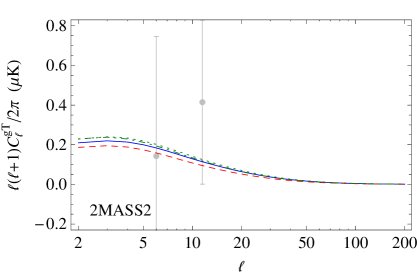
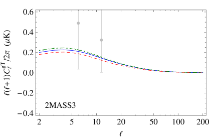
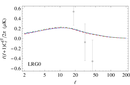
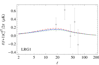
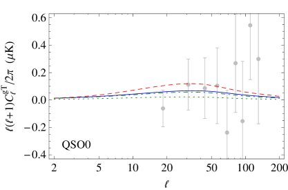
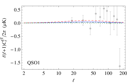
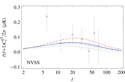
We modify the above calculations in the ISWWLL code with the appropriate DGP quantities such that the correct predictions for the crosscorrelations are obtained. We refer to the Appendix for details. The predictions for the best-fit values, combining all data, of $\Lambda$CDM and sDGP for the different samples are shown in Fig. 3. We also plot the curves for nDGP-B and nDGP-F to illustrate the breaking of the degeneracy between $\Omega_{\Lambda}$ and $\Omega_{K}$. Notice that the model with larger curvature has reduced correlation especially at high redshift. We shall see that models with significantly larger curvature can be excluded by the gISW data.

III.2 Flat universe constraints

We begin by studying a universe without spatial curvature, where the basic cosmological parameter set is $P=\{\Omega_{b}h^{2},\Omega_{c}h^{2},\theta,\tau,n_{s},\ln[10^{10}A_{s}]\}$. We implement the following flat priors on them: $\Omega_{b}h^{2}\in(0.01,0.1)$, $\Omega_{c}h^{2}\in(0.05,0.99)$, $\theta\in(0.5,10)$, $\tau\in(0.01,0.8)$, $n_{s}\in(0.5,1.5)$, and $\ln[10^{10}A_{s}]\in(2.7,4)$. For nDGP and sDGP with nonvanishing $\Lambda$, we use $\Omega_{\Lambda}\in(0.0,2.5)$.

Parameters		$\Lambda$CDM			$\Lambda$CDM (with gISW)
$100\Omega_{b}h^{2}$		$2.248\pm 0.055$	2.240		$2.251\pm 0.055$	2.258
$\Omega_{c}h^{2}$		$0.1080\pm 0.0043$	0.1072		$0.1075\pm 0.0042$	0.1071
$\theta$		$1.0410\pm 0.0027$	1.0404		$1.0411\pm 0.0027$	1.0417
$\tau$		$0.086\pm 0.017$	0.086		$0.087\pm 0.017$	0.089
$n_{s}$		$0.963\pm 0.013$	0.961		$0.963\pm 0.013$	0.965
$\ln[10^{10}A_{s}]$		$3.176\pm 0.041$	3.177		$3.174\pm 0.041$	3.173
$\Omega_{\Lambda}$		$0.751\pm 0.019$	0.754		$0.754\pm 0.019$	0.758
$\Omega_{m}$		$0.249\pm 0.019$	0.246		$0.246\pm 0.019$	0.242
$H_{0}$		$72.6\pm 1.8$	72.6		$72.8\pm 1.8$	73.2
$-2\ln L$		2834.29			2867.99

Table 2: Means, standard deviations (left subdivision of columns), and best-fit values (right subdivision of columns) with likelihood for the flat $\Lambda$CDM model using data from WMAP, ACBAR, CBI, VSA, SNLS, and SHOES without (left column) and with the gISW data (right column).

Parameters		sDGP			sDGP (with gISW)
$100\Omega_{b}h^{2}$		$2.390\pm 0.066$	2.393		$2.390\pm 0.065$	2.376
$\Omega_{c}h^{2}$		$0.0884\pm 0.0042$	0.0873		$0.0889\pm 0.0041$	0.0899
$\theta$		$1.0448\pm 0.0028$	1.0447		$1.0449\pm 0.0028$	1.0452
$\tau$		$0.105\pm 0.021$	0.110		$0.105\pm 0.021$	0.103
$n_{s}$		$1.011\pm 0.015$	1.013		$1.011\pm 0.015$	1.007
$\ln[10^{10}A_{s}]$		$3.001\pm 0.045$	2.998		$3.003\pm 0.044$	3.015
$\Omega_{r_{c}}$		$0.1410\pm 0.0075$	0.1430		$0.1403\pm 0.0075$	0.1384
$\Omega_{m}$		$0.249\pm 0.020$	0.244		$0.251\pm 0.020$	0.256
$H_{0}$		$67.2\pm 1.7$	67.6		$67.1\pm 1.7$	66.7
$-2\Delta\ln L$		32.70			33.06

Table 3: Same as Table 2, but for the flat sDGP model. $-2\Delta\ln L$ is quoted with respect to the maximum likelihood flat $\Lambda$CDM model.

Parameters		sDGP+$\Lambda$			sDGP+$\Lambda$ (with gISW)
$100\Omega_{b}h^{2}$		$2.265\pm 0.058$	2.245		$2.265\pm 0.058$	2.257
$\Omega_{c}h^{2}$		$0.1050\pm 0.0046$	0.1071		$0.1048\pm 0.0046$	0.1070
$\theta$		$1.0415\pm 0.0028$	1.0405		$1.0415\pm 0.0027$	1.0415
$\tau$		$0.089\pm 0.017$	0.080		$0.089\pm 0.017$	0.083
$n_{s}$		$0.969\pm 0.014$	0.961		$0.969\pm 0.014$	0.968
$\ln[10^{10}A_{s}]$		$3.153\pm 0.044$	3.165		$3.152\pm 0.044$	3.154
$\Omega_{\Lambda}$		$0.590-0.752$	0.733		$0.588-0.751$	0.719
$\Omega_{r_{c}}$		$<0.0178$	0.0001		$<0.0186$	0.0003
$\Omega_{m}$		$0.248\pm 0.019$	0.248		$0.247\pm 0.018$	0.247
$H_{0}$		$71.9\pm 1.9$	72.3		$71.9\pm 1.9$	72.5
$-2\Delta\ln L$		0.20			0.13

Table 4: Same as Table 3, but for the flat sDGP+$\Lambda$ model, quoting one-sided 1D marginalized upper 95% CL for $\Omega_{r_{c}}$ and 68% MCI for $\Omega_{\Lambda}$.

Parameters		nDGP			nDGP (with gISW)
$100\Omega_{b}h^{2}$		$2.237\pm 0.054$	2.245		$2.238\pm 0.056$	2.254
$\Omega_{c}h^{2}$		$0.1109\pm 0.0049$	0.1095		$0.1100\pm 0.0046$	0.1076
$\theta$		$1.0406\pm 0.0027$	1.0410		$1.0407\pm 0.0027$	1.0409
$\tau$		$0.084\pm 0.016$	0.084		$0.085\pm 0.017$	0.092
$n_{s}$		$0.958\pm 0.012$	0.961		$0.959\pm 0.013$	0.961
$\ln[10^{10}A_{s}]$		$3.196\pm 0.043$	3.182		$3.191\pm 0.043$	3.190
$\Omega_{\Lambda}$		$0.754-0.934$	0.765		$0.753-0.924$	0.772
$\Omega_{r_{c}}$		$<0.0228$	0.0001		$<0.0203$	0.0001
$\Omega_{m}$		$0.247\pm 0.019$	0.253		$0.243\pm 0.018$	0.244
$H_{0}$		$73.6\pm 2.0$	72.2		$73.9\pm 2.0$	73.0
$-2\Delta\ln L$		0.05			0.23

Table 5: Same as Table 4, but for the flat nDGP model.

We begin with the analysis of flat $\Lambda$CDM without DGP modifications in Table 2. We show constraints with and without the gISW data and the maximum likelihood parameters and value. Horizontal lines divide the chain parameters from the derived parameters and the best-fit (maximum) likelihood. In the case of $\Lambda$CDM, the inclusion of the gISW data does not yield noticeable improvement on the parameter constraints ho:08 . This analysis sets the baseline by which adding the DGP degrees of freedom should be measured.

In the flat sDGP model without $\Lambda$, there is no choice of parameters that can satisfy the joint requirements of geometrical measurements from the CMB, supernovae, and $H_{0}$ and the dynamical requirements from the ISW effect. For sDGP, we find $-2\Delta\ln L=32.7$ with respect to $\Lambda$CDM and $-2\Delta\ln L=33.1$ ($5.8\sigma$) when including the gISW likelihood. In this case, the ISW effect is so large at low multipoles that the CMB alone rules out such contributions fang:08 and the gISW constraint adds only an insignificant amount of extra information (see Tables 3). The strengthening of the constraint when compared to Ref. fang:08 comes from the improved Hubble constant measurements.

In the sDGP+$\Lambda$ and nDGP models, the cosmological constant becomes a free parameter and we have to add it to the parameter set, hence, $P\rightarrow P\ \cup\ \{\Omega_{\Lambda}\}$. $\Omega_{r_{c}}$ is a derived parameter and in particular we get $\Omega_{r_{c}}\rightarrow 0$ in the limit $\Omega_{\Lambda}\rightarrow(1-\Omega_{m})$. In this limit, the phenomenology of $\Lambda$CDM is recovered for all observables. Preference for a finite $\Omega_{r_{c}}$ indicates evidence for the DGP modification in these cases.

In both the nDGP and sDGP+$\Lambda$ cases the maximum likelihood models differ insignificantly from $\Lambda$CDM (see Tables 4 and 5) and there is no preference for finite $\Omega_{r_{c}}$. Conversely, both branches require a finite $\Omega_{\Lambda}$ at high significance.

Since $\Lambda$CDM is the $\Omega_{r_{c}}\rightarrow 0$ limit of both branches with $\Lambda$, the slightly poorer fit for nDGP and sDGP+$\Lambda$ should be attributed to sampling error in the MCMC. The one-sided 1D marginalized upper 95% confidence limits for $\Omega_{r_{c}}$ are $\Omega_{r_{c}}<0.0178(0.0186)$ for sDGP+$\Lambda$ and $\Omega_{r_{c}}<0.0228(0.0203)$ for nDGP where the values in parentheses include the gISW constraint. These values indicate that the crossover scale is at least substantially greater than the Hubble scale $H_{0}r_{c}\gtrsim 3.5$.

In this $\Lambda$CDM limit, the modifications to the gISW predictions do not affect the constraints. The slight weakening of the constraints with the inclusion of gISW in sDGP+$\Lambda$ does not indicate a statistically significant tension but does suggest that future improvement in constraints can tighten the bounds on $H_{0}r_{c}$. In particular, sDGP modifications tend to enhance correlations at high redshift relative to low redshift. The current data have a marginal preference for increased correlation with redshift relative to $\Lambda$CDM (see Fig. 3).

Note that due to the distinctive skewness of the posterior distribution, we give the 1D marginalized 68% minimum credible intervals (MCI) (see Ref. hamann:07 ) for the brane tension $\Omega_{\Lambda}$ as opposed to the standard deviations given for the other parameters.

Finally, in the context of these flat models the possibility of phantom equations of state currently is highly constrained. For nDGP $1+w_{0}>-0.039$ at the 95% C.L.

III.3 Nonflat universe constraints

In a universe with spatial curvature, we include $\Omega_{K}$ as a parameter in the chain for each of the model classes. We use the prior $\Omega_{K}\in(-0.1,0.1)$, which we weaken to $\Omega_{K}\in(-1,1)$ in nDGP since we expect degeneracies between $\Omega_{K}$ and $\Omega_{\Lambda}$. We also implement latter prior for sDGP+$\Lambda$. For $\Lambda$CDM, Ho et al. ho:08 have found an improvement of the constraints on $\Omega_{K}$ by a factor of 3.2, with respect to WMAP3 data alone, due to the inclusion of the gISW and weak lensing data. However we find that the inclusion of the other data, specifically the supernova and $H_{0}$ data, make curvature constraints only marginally improved by the gISW inclusion. We again use these $\Lambda$CDM results shown in Table 6 as a baseline for comparison with sDGP, sDGP+$\Lambda$, and nDGP in Tabsles 7, 8, and 9.

For sDGP without $\Lambda$, adding curvature alleviates the tension between CMB and supernova distance measures. However, it cannot reduce the ISW contributions song:06 ; fang:08 and so we obtain $-2\Delta\ln L=23.3(23.8)$, with respect to $\Lambda$CDM where values in parentheses include the gISW constraint. Utilizing all of the data, the significance of the exclusion of sDGP without $\Lambda$ is $\sim 5\sigma$.

Similar to the flat case, we find no preference for a finite $\Omega_{r_{c}}$ in nDGP and sDGP+$\Lambda$ and consequently no indications of DGP modifications to gravity (see Fig. 4). With sDGP+$\Lambda$, we are again driven to the limiting case of $\Lambda$CDM with the slightly poorer best fit reflecting a sampling error in the chain. Allowance for curvature on the other hand weakens the upper limit on the DGP modifications: $\Omega_{r_{c}}<0.0248(0.0244)$ and $H_{0}r_{c}>3.18(3.20)$ at 95% C.L.

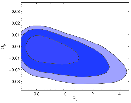
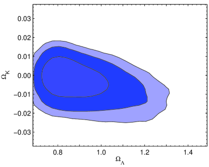
For nDGP, the addition of curvature introduces a degeneracy with the cosmological constant. As was pointed out by Giannantonio et al. giannantonio:08 , this degeneracy can be broken by the use of galaxy-ISW cross correlations since high curvature solutions underpredict the correlation especially at high redshift. Figure 5 illustrates this degeneracy and the effect of gISW measures. The result of marginalizing curvature in nDGP is again a weakening of the DGP constraints $\Omega_{r_{c}}<0.0501(0.0300)$ and $H_{0}r_{c}>2.23(2.89)$ at 95% C.L.

In summary with the gISW constraint, the limit on either branch implies $H_{0}r_{c}\gtrsim 3$ and only a small weakening from the flat case of $3.5$. Furthermore due to the curvature degeneracy in nDGP, restrictions on phantomlike equations of state are also somewhat weakened to $w_{0}+1<-0.049$.

Figure 4: Marginalized likelihood for $\Omega_{r_{c}}$ in the nonflat nDGP and sDGP models. The vertical lines indicate 68%, 95%, and 99% C.L.

Figure 5: Contours of 2D marginalized 68%, 95%, and 99% confidence boundaries using WMAP5, ACBAR, CBI, VSA, SNLS, and SHOES (left panel), including gISW (right panel) for nDGP.

Parameters		$\Lambda$CDM			$\Lambda$CDM (with gISW)
$100\Omega_{b}h^{2}$		$2.250\pm 0.056$	2.246		$2.249\pm 0.055$	2.238
$\Omega_{c}h^{2}$		$0.1084\pm 0.0052$	0.1095		$0.1084\pm 0.0051$	0.1085
$\theta$		$1.0412\pm 0.0027$	1.0412		$1.0411\pm 0.0027$	1.0419
$\tau$		$0.086\pm 0.017$	0.090		$0.087\pm 0.017$	0.083
$n_{s}$		$0.963\pm 0.013$	0.960		$0.963\pm 0.013$	0.962
$\ln[10^{10}A_{s}]$		$3.176\pm 0.044$	3.196		$3.179\pm 0.043$	3.174
$\Omega_{K}$		$-0.0001\pm 0.0063$	0.0020		$0.0007\pm 0.0062$	0.0021
$\Omega_{\Lambda}$		$0.751\pm 0.020$	0.751		$0.753\pm 0.019$	0.758
$\Omega_{m}$		$0.249\pm 0.022$	0.246		$0.246\pm 0.022$	0.240
$H_{0}$		$72.6\pm 3.0$	73.2		$73.0\pm 3.0$	73.8
$-2\ln L$		2834.01			2867.74

Table 6: $\Lambda$CDM as in Table 2, except allowing spatial curvature.

Parameters		sDGP			sDGP (with gISW)
$100\Omega_{b}h^{2}$		$2.377\pm 0.061$	2.365		$2.376\pm 0.062$	2.352
$\Omega_{c}h^{2}$		$0.0951\pm 0.0041$	0.0970		$0.0952\pm 0.0039$	0.0979
$\theta$		$1.0441\pm 0.0028$	1.0451		$1.0441\pm 0.0028$	1.0439
$\tau$		$0.091\pm 0.020$	0.084		$0.092\pm 0.019$	0.084
$n_{s}$		$1.004\pm 0.014$	1.002		$1.004\pm 0.014$	0.997
$\ln[10^{10}A_{s}]$		$3.018\pm 0.043$	3.019		$3.021\pm 0.043$	3.037
$\Omega_{K}$		$0.0186\pm 0.0055$	0.0212		$0.0182\pm 0.0055$	0.0220
$\Omega_{r_{c}}$		$0.1486\pm 0.0068$	0.1486		$0.1479\pm 0.0067$	0.1467
$\Omega_{m}$		$0.218\pm 0.019$	0.216		$0.220\pm 0.019$	0.220
$H_{0}$		$74.0\pm 3.0$	74.7		$73.7\pm 2.9$	74.2
$-2\Delta\ln L$		23.32			23.79

Table 7: sDGP without $\Lambda$ as in Table 3, except allowing spatial curvature. $-2\Delta\ln L$ is quoted with respect to the maximum likelihood $\Lambda$CDM model with curvature here and in the following tables.

Parameters		sDGP+$\Lambda$			sDGP+$\Lambda$ (with gISW)
$100\Omega_{b}h^{2}$		$2.266\pm 0.058$	2.252		$2.266\pm 0.0059$	2.251
$\Omega_{c}h^{2}$		$0.1065\pm 0.0051$	0.1066		$0.1064\pm 0.0051$	0.1095
$\theta$		$1.0416\pm 0.0028$	1.0406		$1.0415\pm 0.0028$	1.0414
$\tau$		$0.087\pm 0.017$	0.077		$0.088\pm 0.017$	0.090
$n_{s}$		$0.968\pm 0.014$	0.962		$0.968\pm 0.014$	0.960
$\ln[10^{10}A_{s}]$		$3.157\pm 0.046$	3.153		$3.158\pm 0.046$	3.197
$\Omega_{K}$		$0.0032\pm 0.0068$	0.0022		$0.0036\pm 0.0065$	0.0018
$\Omega_{\Lambda}$		$0.557-0.745$	0.711		$0.561-0.746$	0.737
$\Omega_{r_{c}}$		$<0.0248$	0.0006		$<0.0244$	0.0000
$\Omega_{m}$		$0.245\pm 0.022$	0.240		$0.243\pm 0.021$	0.248
$H_{0}$		$72.8\pm 3.0$	73.3		$73.1\pm 2.9$	72.9
$-2\Delta\ln L$		0.07			0.04

Table 8: sDGP with $\Lambda$ as in Table 4, but allowing spatial curvature.

Parameters		nDGP			nDGP (with gISW)
$100\Omega_{b}h^{2}$		$2.239\pm 0.056$	2.245		$2.242\pm 0.056$	2.239
$\Omega_{c}h^{2}$		$0.1099\pm 0.0054$	0.1076		$0.1094\pm 0.0054$	0.1099
$\theta$		$1.0409\pm 0.0027$	1.0412		$1.0409\pm 0.0027$	1.0409
$\tau$		$0.084\pm 0.017$	0.084		$0.085\pm 0.017$	0.091
$n_{s}$		$0.959\pm 0.013$	0.960		$0.960\pm 0.013$	0.960
$\ln[10^{10}A_{s}]$		$3.189\pm 0.045$	3.176		$3.188\pm 0.045$	3.205
$\Omega_{K}$		$-0.0055\pm 0.0080$	-0.0056		$-0.0029\pm 0.0069$	0.0021
$\Omega_{\Lambda}$		$0.749-1.009$	0.801		$0.749-0.953$	0.764
$\Omega_{r_{c}}$		$<0.0501$	0.0008		$<0.0300$	0.0000
$\Omega_{m}$		$0.255\pm 0.023$	0.261		$0.248\pm 0.022$	0.247
$H_{0}$		$72.1\pm 3.0$	70.6		$73.0\pm 3.0$	73.1
$-2\Delta\ln L$		0.09			0.41

Table 9: nDGP as in Table 5, but allowing spatial curvature.

IV Discussion

We have performed the first Markov chain Monte Carlo analysis of the nDGP and sDGP branches of DGP braneworld gravity to utilize all of the CMB data, including the lowest multipoles, and its correlation with galaxies (gISW). We also include supernovae and Hubble constant data in the constraint.

We find no preference for DGP modifications to gravity on either branch. Indeed, on the self-accelerating branch without $\Lambda$, the model is excluded at the $4.9\sigma$ and $5.8\sigma$ levels with and without curvature respectively fang:08 . While the gISW data do not substantially improve this constraint, they do additionally disfavor sDGP.

With the inclusion of $\Lambda$ on either branch, the DGP model cannot be entirely excluded but its modifications are strongly limited. We find that the crossover scale, which measures the strength of the modifications, must be substantially above the Hubble scale $H_{0}r_{c}>3$ with curvature and $3.5$ without curvature. The robustness of this constraint is substantially assisted by the gISW data. In nDGP, it breaks the geometric degeneracy between $\Lambda$ and spatial curvature. In sDGP, the relatively large correlation at high redshift offers opportunities in the future for improving the limits on $H_{0}r_{c}$. These abilities highlight the importance of obtaining improved gISW data for constraining infrared modifications to gravity.

Appendix A Modifications to the ISWWLL code

We use the publicly available ISWWLL code ho:08 ; hirata:08 for our analysis. Note that we have turned off weak lensing likelihood contributions in the code, focusing only on the gISW constraints. The 42 data points of gISW cross correlations that are used in the likelihood analysis are collected from the Two Micron All Sky Survey (2MASS) extended source catalog (XSC) jarrett:00 ; skrutskie:06 , the luminous red galaxies (LRG) and photometric quasars (QSO) of the Sloan Digital Sky Survey (SDSS) adelman:07 , and the National Radio Astronomy Observatory (NRAO) Very Large Array (VLA) Sky Survey (NVSS) condon:98 . They are divided into nine galaxy sample bins $j$ (2MASS0-3, LRG0-1, QSO0-1, NVSS) based on flux (2MASS) or redshift (LRG, QSO). These data points are a selection of multipole bins from all samples, where the selection is based on the avoidance of nonlinearities and systematic effects from dust extinction, galaxy foregrounds, the thermal Sunyaev-Zel’dovich effect, and point source contamination to affect the gISW cross correlations ho:08 .

In the remainder of this Appendix, we discuss the details of the modifications implemented in the ISWWLL code. First, we describe the calculation of the quasistatic linear growth rate $D(z)$ in the gISW cross correlation, Eq. (21), and analyze the validity of the Limber and the quasistatic approximation. We then discuss the function $f_{j}(z)$ that carries information about the redshift distribution and bias.

A.1 gISW cross correlations

It has been argued that for nDGP and sDGP the gISW cross correlations are well described within the quasistatic regime song:06 ; giannantonio:08 ; koyama:05 ; sawicki:06 . Here, this can easily be seen from the substitution $k\rightarrow(\ell+1/2)/\chi(z)$ considering the relevant redshifts. In this limit, we solve the ordinary differential equation lue:04

$$\Delta_{m}^{\prime\prime}+\left(2+\frac{H^{\prime}}{H}\right)\Delta_{m}^{\prime}-\frac{3}{2}\left(1-g_{\rm QS}\right)\frac{H_{0}^{2}\Omega_{m}}{a^{3}H^{2}}\Delta_{m}=0$$ (22)

for the linear matter density perturbation $\Delta_{m}$. Note that for nDGP, in the limit $r_{c}\rightarrow\infty$, we have $g_{\rm QS}\rightarrow 0$ and $H(z)$ approaches the expansion history of $\Lambda$CDM. Therefore, in this limit, Eq. (22) recovers the quasistatic ordinary differential equation for the matter overdensity in $\Lambda$CDM. We solve Eq. (22) with initial conditions at $a_{i}\ll 1$, in a regime where general relativity is expected to hold, i.e., $\Delta_{m}^{\prime}(a_{i})=\Delta_{m}(a_{i})$ with a normalization set by the initial power spectrum.

The accuracy of the Limber approximation in the case of $\Lambda$CDM is at the order of 10% at $\ell=2$ and drops approximately as $\ell^{2}$ at higher $\ell$ (see e.g. smith:09 ; loverde:08 ; afshordi:04 ). The error depends further on the width of the redshift distribution, which changes only little with DGP effects. The relative deviation from the exact result at $\ell=6$ does not exceed $\sim 3\%$ for the samples and typical models considered in Fig. 3. Given the large errors of the currently available data points at low $\ell$, we conclude that the Limber approximation is applicable and furthermore very useful since it is numerically faster than an exact integration.

A.2 Redshift distribution and bias

A further modification to the code that we need to conduct is in the determination of the function $f_{j}(z)$. In the Markov chain, $f_{j}(z)$ is recomputed when changing the cosmological parameter values. The methods by which this function is determined differ for each sample, but they are all based on galaxy clustering data.

The 2MASS galaxies are matched with SDSS galaxies in order to identify their redshifts. To obtain the nonlinear power spectrum, the $Q$ model for nonlinearities cole:05 is applied. Then, the code computes the galaxy power spectrum and fits it to measurements, thereby determining the bias $b(z)$ and $Q$. Since the required accuracy for the estimation of bias is only at the order of a few tens of percent ho:08 , this processing is also applicable to DGP. The $Q$ model is also adopted for LRG galaxies, where the redshift probability distribution is inferred with methods described in Ref. padmanabhan:05 . For QSO, first, a preliminary estimate for the redshift distribution is deduced by locating a region of sky with high spectroscopic completeness, but simultaneously maintaining a large area. Taking into account magnification bias and fitting $b_{j}(z)\Pi_{j}(z)$ using the quasar power spectrum and quasar-LRG cross power yields the desired shape of $f_{j}(z)$. Finally, the effective redshift distribution of NVSS is obtained from cross-correlating with the other samples and $f_{j}(z)$ is fitted with a $\Gamma$ distribution.

The part of the ISWWLL code that is devoted to this processing is configured for a parametrization of the expansion history by $w_{e}=w_{0}+(1-a)w_{a}$. This approach gives a good approximation to sDGP in the domain of interest, but it fails for nDGP and sDGP+$\Lambda$ due to the appearance of a divergence in $w_{e}(a)$. Therefore, instead of taking $w_{0}$ and $w_{a}$ to describe the expansion history, we utilize $\Omega_{r_{c}}$ and $\Omega_{\Lambda}$, where only the latter really is a necessary, free parameter.

In case of the SDSS quasars, the derivation of $f_{j}(z)$ involves the linear growth factor, which we need to replace by its DGP counterpart. This implies solving Eq. (22). A further contribution for the QSO samples is due to magnification bias. In the quasistatic regime of DGP the relationship between the metric combination sensitive to gravitational redshifts and lensing ($\Phi-\Psi$) and the density perturbations is unmodified so the expression of the lensing window function for magnification effects given in Ref. ho:08 is unchanged.

References

- (1) G. R. Dvali, G. Gabadadze and M. Porrati, Phys. Lett. B485, 208 (2000), [arXiv:hep-th/0005016].
- (2) C. Deffayet, Phys. Lett. B502, 199 (2001), [arXiv:hep-th/0010186].
- (3) M. Fairbairn and A. Goobar, Phys. Lett. B 642, 432 (2006), [arXiv:astro-ph/0511029].
- (4) R. Maartens and E. Majerotto, Phys. Rev. D 74, 023004 (2006), [arXiv:astro-ph/0603353].
- (5) W. Fang et al., Phys. Rev. D78, 103509 (2008), [arXiv:0808.2208].
- (6) M. A. Luty, M. Porrati and R. Rattazzi, JHEP 09, 029 (2003), [arXiv:hep-th/0303116].
- (7) C. Charmousis, R. Gregory, N. Kaloper and A. Padilla, JHEP 10, 066 (2006), [arXiv:hep-th/0604086].
- (8) G. Dvali, New J. Phys. 8, 326 (2006), [arXiv:hep-th/0610013].
- (9) K. Koyama, Class. Quant. Grav. 24, R231 (2007), [arXiv:0709.2399].
- (10) V. Sahni and Y. Shtanov, JCAP 0311, 014 (2003), [arXiv:astro-ph/0202346].
- (11) W. Hu and I. Sawicki, Phys. Rev. D76, 104043 (2007), [arXiv:0708.1190].
- (12) W. Hu, Phys. Rev. D77, 103524 (2008), [arXiv:0801.2433].
- (13) W. Fang, W. Hu and A. Lewis, Phys. Rev. D78, 087303 (2008), [arXiv:0808.3125].
- (14) Y.-S. Song, I. Sawicki and W. Hu, Phys. Rev. D75, 064003 (2007), [arXiv:astro-ph/0606286].
- (15) Y.-S. Song, Phys. Rev. D77, 124031 (2008), [arXiv:0711.2513].
- (16) T. Giannantonio, Y.-S. Song and K. Koyama, Phys. Rev. D78, 044017 (2008), [arXiv:0803.2238].
- (17) S. Ho, C. Hirata, N. Padmanabhan, U. Seljak and N. Bahcall, Phys. Rev. D78, 043519 (2008), [arXiv:0801.0642].
- (18) C. M. Hirata, S. Ho, N. Padmanabhan, U. Seljak and N. A. Bahcall, Phys. Rev. D78, 043520 (2008), [arXiv:0801.0644].
- (19) I. Sawicki, Y.-S. Song and W. Hu, Phys. Rev. D75, 064002 (2007), [arXiv:astro-ph/0606285].
- (20) A. Lewis, A. Challinor and A. Lasenby, Astrophys. J. 538, 473 (2000), [arXiv:astro-ph/9911177].
- (21) S. Seahra, W. Hu and Y.-S. Song, in preparation (2009).
- (22) A. Cardoso, K. Koyama, S. S. Seahra and F. P. Silva, Phys. Rev. D77, 083512 (2008), [arXiv:0711.2563].
- (23) N. Afshordi, G. Geshnizjani and J. Khoury, arXiv:0812.2244.
- (24) WMAP, J. Dunkley et al., Astrophys. J. Suppl. 180, 306 (2009), [arXiv:0803.0586].
- (25) C.-L. Kuo et al., Astrophys. J. 664, 687 (2007), [arXiv:astro-ph/0611198].
- (26) A. C. S. Readhead et al., Astrophys. J. 609, 498 (2004), [arXiv:astro-ph/0402359].
- (27) K. Grainge et al., Mon. Not. Roy. Astron. Soc. 341, L23 (2003), [arXiv:astro-ph/0212495].
- (28) The SNLS, P. Astier et al., Astron. Astrophys. 447, 31 (2006), [arXiv:astro-ph/0510447].
- (29) A. G. Riess et al., Astrophys. J. 699, 539 (2009), [arXiv:0905.0695].
- (30) A. Lewis and S. Bridle, Phys. Rev. D66, 103511 (2002), [arXiv:astro-ph/0205436].
- (31) J. Hamann, S. Hannestad, G. G. Raffelt and Y. Y. Y. Wong, JCAP 0708, 021 (2007), [arXiv:0705.0440].
- (32) T. H. Jarrett et al., Astron. J. 119, 2498 (2000), [arXiv:astro-ph/0004318].
- (33) M. F. Skrutskie et al., Astron. J. 131, 1163 (2006).
- (34) SDSS, J. K. Adelman-McCarthy et al., Astrophys. J. Suppl. 175, 297 (2008), [arXiv:0707.3413].
- (35) J. J. Condon et al., Astron. J. 115, 1693 (1998).
- (36) K. Koyama and R. Maartens, JCAP 0601, 016 (2006), [arXiv:astro-ph/0511634].
- (37) A. Lue, R. Scoccimarro and G. D. Starkman, Phys. Rev. D69, 124015 (2004), [arXiv:astro-ph/0401515].
- (38) R. E. Smith, C. Hernandez-Monteagudo and U. Seljak, arXiv:0905.2408.
- (39) M. LoVerde and N. Afshordi, Phys. Rev. D78, 123506 (2008), [arXiv:0809.5112].
- (40) N. Afshordi, Phys. Rev. D70, 083536 (2004), [arXiv:astro-ph/0401166].
- (41) The 2dFGRS, S. Cole et al., Mon. Not. Roy. Astron. Soc. 362, 505 (2005), [arXiv:astro-ph/0501174].
- (42) SDSS, N. Padmanabhan et al., Mon. Not. Roy. Astron. Soc. 359, 237 (2005), [arXiv:astro-ph/0407594].