Grand-canonical and canonical solution of self-avoiding walks with up to 3 monomers per site on the Bethe lattice

Abstract

We solve a model of polymers represented by self-avoiding walks on a lattice which may visit the same site up to three times in the grand-canonical formalism on the Bethe lattice. This may be a model for the collapse transition of polymers where only interactions between monomers at the same site are considered. The phase diagram of the model is very rich, displaying coexistence and critical surfaces, critical, critical endpoint and tricritical lines, as well as a multicritical point. From the grand-canonical results, we present an argument to obtain the properties of the model in the canonical ensemble, and compare our results with simulations in the literature. We do actually find extended and collapsed phases, but the transition between them, composed by a line of critical endpoints and a line of tricritical points, separated by the multicritical point, is always continuous. This result is at variance with the simulations for the model, which suggest that part of the line should be a discontinuous transition. Finally, we discuss the connection of the present model with the standard model for the collapse of polymers (self-avoiding self-attracting walks), where the transition between the extended and collapsed phases is a tricritical point.

I Introduction

Polymers may be modelled as self-avoiding walks on a lattice. Each walk visits a sequence of first-neighbor lattice sites and may be viewed as a chain of monomers located on the lattice sites linked by bonds on the lattice edges. This model was already considered by Flory in his pioneering work on polymers f66 , and later De Gennes discovered a mapping between this model and the $n$-vector model of magnetism in the formal limit $n\to 0$, which allowed him to apply the renormalization group formalism to this problem dg72 . The ideas of scaling and universality are very important in this field dg79 .

If the polymer is placed in a poor solvent, the interactions between the molecules (monomer-monomer, monomer-solvent, and solvent-solvent) penalize energetically the monomer-solvent contacts. In a lattice model, this may be studied considering an effective attractive interactions between monomers located on first-neighbor sites of the lattice which are not consecutive along a chain. These interactions compete with the repulsive excluded volume interactions (which lead to the self-avoidance constraint), and at sufficiently low temperatures the chain may undergo a collapse transition, from an extended to a more compact configuration. For example, the exponent $\nu$ which describes the behavior of the mean square end-to-end distance of the chain as a function of the molecular weight (number of monomers) $M$, $\langle R^{2}\rangle\approx M^{2\nu}$, changes from a larger value in the extended configuration to $1/d$, where $d$ is the dimensionality of the lattice, in the collapsed state. The temperature at which this transition happens is called the $\theta$-temperature f66 . It turns out to be particularly interesting to consider this model of self-attracting self-avoiding walks (SASAW’s) in the grand-canonical ensemble dg79 , since the polymerization transition in the chemical potential $\times$ temperature phase diagram is found to change from continuous, at high temperatures to discontinuous below the $\theta$-temperature. This is consistent with the description of the behavior of the exponent $\nu$ above, since at the transition the density of monomers vanishes for $T>T_{\theta}$ and is finite for $T<T_{\theta}$. Thus, the $\theta$-point may be recognized as a tricritical point. Much is known about this tricritical point in two dimensions ds85 and its exact tricritical exponents were found through the study of a diluted polymerization model ds87 . On the square lattice, for a model where the attractive interactions are between bonds of the chain on opposite edges of elementary squares, there are indications that an even richer phase diagram is found, with an additional dense polymerized phase sms96 ; p02 .

Some time ago, a model was introduced to study interacting polymers where only one-site interactions are present kpor06 , in opposition to the usual SASAW’s model, where we have interactions between monomers at first-neighbor sites. Usually lattice models for fluids may be viewed as a consequence of the partition of space into small cells (cellular model), of molecular size. In the SASAW’s model, such a cell may be occupied by a single monomer or empty. Now if the cells are larger, they may be occupied by more than one monomer (we will call this the multiple monomers per site (MMS) model) , and the interactions may be supposed to occur only between monomers in the same cell. If the bonds are larger than the size of the cells, two monomers in the same cell may not be connected by a bond. Thus, in the new model each lattice site may be either empty or occupied by $1,2,\ldots,K$ monomers, and an attractive interaction exists between each pair of monomers on the same site. This model may be viewed as a generalization of the Domb-Joyce model, where also multiple monomers may be placed on the same lattice site dj72 . In kpor06 two versions of the model were studied using canonical simulations: in the RA (immediate reversals allowed) model there are no additional restrictions on the walks, but in the RF (immediate reversals forbidden) model configurations where the walk leaves one site, reaches a first neighbor and returns to the original site are not allowed. The simulation lead to particularly interesting results for the RF model on the cubic lattice, with two distinct collapse transitions present in the phase diagram. The precise nature of these transitions, as well as the nature of the multicritical point where the two transition lines meet, could not be found, although one of the collapse transitions seems to be discontinuous.

Recently, the RF and RA models in the grand-canonical ensemble were solved on the Bethe lattice ss07 for the case $K=2$. The parameter space for this model is defined by the statistical weights $\omega_{i}$, $i=1,2$, of sites occupied by $i$ monomers (the weight of empty sites is equal to one). In the solution of the RF model the continuous polymerization transition at high temperatures ended at a tricritical point, similar to what is observed for the SASAW’s model. An additional polymerized phase (DO) appears at higher values of the statistical weight of double occupied sites $\omega_{2}$, where only empty and double-occupied sites are present. Later, the RF model, still for $K=2$, was solved on the Husimi lattice oss08 . It is expected that this solution should be closer to the thermodynamic behavior observed on regular lattices. The phase diagram found is similar to the one obtained in the Bethe lattice solution, although the region of stability of the DO phase is smaller. It is also worth to mention that a rather unphysical result found on the Bethe lattice, where the tricritical collapse transition point is found for vanishing interactions between monomers, is corrected in the Husimi lattice, where this point is located in the region of attractive interactions, as expected.

In this paper we solve the model for $K=3$ on the Bethe lattice. This generalization of the previous work allows us to compare our results with the simulations described by Krawczyk et al kpor06 . Actually, the correspondence between the canonical ensemble, in which the simulations were done, and the grand-canonical ensemble used in this paper is not straightforward for the polymer models, and we will discuss this matter in detail below. Basically, to compare the grand-canonical results to the behavior of the model in the canonical situation, we consider that when the polymers are placed in an excess of solvent (dilute situation), we actually have them coexisting with the pure solvent phase, which corresponds to the non-polymerized phase, stable in the grand-canonical solution for low values of the monomer activity. The density of the coexisting polymer phase may vanish, and therefore we have a critical situation associated to extended polymers, or may be finite, corresponding to collapsed polymers. In the present calculations, we considered the monomers located on the same site to be indistinguishable, as was done in the previous work oss08 , and in opposition to the calculations done in ss07 , where the distinguishable case was treated. One of the reasons to do so is that the simulations presented in kpor06 were also performed for the indistinguishable case. Another additional point which we address is the location of coexistence surfaces in the phase diagram of models solved on hierarchical lattices such as the Bethe lattice. In the previous calculations of the MMS model on treelike lattices, the recursion relations were used directly to find the coexistence loci iterating them with initial conditions defined by the parameters of the model, a procedure proposed in p02 . Although this procedure has considerable physical appeal, it is not granted that the results furnished by it will be consistent with the ones provided by free-energy calculations. Actually, in more complex models the ‘natural’ initial conditions (NIC) may not be unique and there is the possibility that different locations for the coexistence surface are obtained for different reasonable choices of these conditions. Therefore, in the present calculations we decided to adopt a definition for the bulk free energy per site which was proposed some time ago by Gujrati g95 and has lead to the same results as other methods based on more solid foundations, such as the integration over the order parameter, in models where it is possible to perform these calculations. We found that in the present model the revision of the procedure to find the coexistence surfaces actually lead to qualitative changes in the phase diagram, thus showing that the NIC method adopted before may actually lead to results which are not close to the ones provided by more reliable calculations.

In section II the model is defined in more detail and its solution on the Bethe lattice is obtained. The thermodynamic behavior of the model is presented in section III. In section IV, we discuss the relation between the grand-canonical and the canonical behavior of the model, comparing the results of the present calculation with the finding of the simulations performed by Krawczyk et al kpor06 . Final discussions may be found in section V. Some more results and discussions concerning the location of coexistence surfaces on Bethe lattice solutions have been placed in the appendix A, and the determination of the multicritical point in the parameter space may be found in the appendix B.

II Definition of the model and solution in terms of recursion relations

We consider self- and mutually avoiding walks on a Cayley tree with arbitrary coordination number $q$, imposing the constraint which forbids immediate reversals. The endpoints of the walks are placed on the surface of the tree. The grand-canonical partition function of the model will be given by:

$$Y=\sum\omega_{1}^{N_{1}}\omega_{2}^{N_{2}}\omega_{3}^{N_{3}}$$ (1)

where the sum is over the configurations of the walks on the tree, while $N_{i}$ , $i=1,2,3$ is the number of sites visited $i$ times by the walks or, in other words, the number of sites with $i$ monomers in the configuration. Thus, $\omega_{i}$, $i=1,2,3$ are the statistical weights of a site visited $i$ times or, in other words, with $i$ monomers placed on them. In Fig. 1 a contribution to the partition function is shown.

Figure 1: (Color online) A contribution to the partition function of the model on a Cayley tree with $q=4$ and 3 generations. The weight of this contribution will be $\omega_{1}^{6}\omega_{2}^{3}\omega_{3}^{4}$.

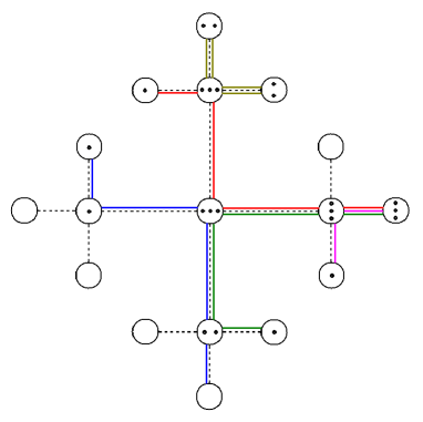
As usual, to solve the model on the Bethe lattice we start considering rooted subtrees of the Cayley tree, defining partial partition functions for them, where we sum over all possible configurations for a fixed configuration of the root of the subtree. We thus define four partial partition functions $g_{i}$ , $i=0,1,2,3$, where $i$ corresponds to the number of polymer bonds placed on the root edge of the subtree. The subtrees are shown in Fig. 2.

Figure 2: Illustration of the rooted subtrees which correspond to the partial partition functions.

Actually, it is important to discuss a point about these choice for the partial partition functions. For the ones with multiple bonds at the root edge ($g_{2}$ and $g_{3}$) a distinction should be made between the situations where two or more bonds are distinguishable or not, since this distinction is important when we will define the combinatorial coefficients in the recursion relations below. A pair of bonds which are indistinguishable corresponds to the situation where both chains visit the same sequence of sites since the surface of the tree. Therefore, $g_{2}$ should be split into two different partial partition functions and three cases should be considered for $g_{3}$. Thus, the total number of partial partition functions would be equal to seven. However, we found out that it is sufficient to consider only the case where all bonds are distinguishable, since the ratios of $g_{i}/g_{0}$ where $g_{i}$ is a partial partition function of a configuration with indistinguishable bonds all vanish at the relevant fixed points of the recursion relations defined below, which corresponds to the thermodynamic behavior of the model. Actually, there are two fixed points where the density of edges with one polymer bond on them vanishes, and for the phases associated to these fixed points (the DO and TO fixed points described below) the inclusion of indistinguishable polymer bonds in the recursion relations leads to different results, since their density does not vanish in the thermodynamic limit. However, we found that these phases will never be the one with lowest free energy in any point of the parameter space, and thus if we do not include indistinguishable bonds in our discussion this will not imply any change in the phase diagram. Therefore, we decided, for simplicity, to restrict the discussion of the model to the case of distinguishable bonds only. In other words, in the limit of an infinite tree, chains with indistinguishable bonds will never reach the central region of the tree if the density of edges with single polymer bonds does not vanish in this region. This may be understood if we notice that in the recursion relations for partial partition functions with indistinguishable bonds there are always configurations connecting them to other configurations without those bonds, provided single bonds are incident at the same site, but never the opposite happens, so it is not surprising that these contributions vanish at the fixed points. We will discuss this point in some more detail below, when the recursion relations for the partial partition functions will be obtained. Also, we notice that if we would adopt that the surface sites of the tree should not be occupied by two monomers, we never would have indistinguishable bonds at any stage of the iteration, but in treelike structures like the Bethe lattice it is not granted that such a constraint will not influence the phase diagram of the model.

We then proceed obtaining recursion relations for the partial partition functions, by considering the operation of attaching $q-1$ subtrees with a certain number of generations to a new root site and edge, thus building a subtree with an additional generation. Below the recursion relations are presented. In general, we have $g^{\prime}_{i}=\sum_{j}g^{\prime}_{i,j}$ , where the primes denote the partial partition function on the subtree with one more generation. Whenever appropriate, the contributions to the sums begin with a product of two numerical factors, the first of which is the multiplicity of the configuration of the incoming bonds and the second is the multiplicity of the connections with the monomers located at the new site. As discussed in the introduction, we consider the monomers to be indistinguishable, in opposition to what we did in the particular case $K=2$ of the RF model we have studied before ss07 . Actually, in the recursion relations below, to obtain the results for the case of distinguishable monomers one simply has to replace $\omega_{2}$ by $2\omega_{2}$ and $\omega_{3}$ by $6\omega_{3}$. The recursion relation for $g_{0}$ is the sum of the contributions:

$$g^{\prime}_{0,1} = g_{0}^{q-1},$$ (2a)

$$g^{\prime}_{0,2}\, = \,\binom{q-1}{2}\times 1\,\omega_{1}\,g_{0}^{q-3}\,g_{1}^{2},$$ (2b)

$$g^{\prime}_{0,3}\, = \,\binom{q-1}{4}\times 3\,\omega_{2}\,g_{0}^{q-5}\,g_{1}^{4},$$ (2c)

$$g^{\prime}_{0,4}\, = \,3\,\binom{q-1}{3}\times 2\,\omega_{2}\,g_{0}^{q-4}\,g_{1}^{2}\,g_{2},$$ (2d)

$$g^{\prime}_{0,5}\, = \,\binom{q-1}{2}\times 2\,\omega_{2}\,g_{0}^{q-3}\,g_{2}^{2},$$ (2e)

$$g^{\prime}_{0,6}\, = \,\binom{q-1}{6}\times 15\,\omega_{3}\,g_{0}^{q-7}\,g_{1}^{6},$$ (2f)

$$g^{\prime}_{0,7}\, = \,5\,\binom{q-1}{5}\times 12\,\omega_{3}\,g_{0}^{q-6}\,g_{1}^{4}\,g_{2},$$ (2g)

$$g^{\prime}_{0,8}\, = \,6\,\binom{q-1}{4}\times 10\,\omega_{3}\,g_{0}^{q-5}\,g_{1}^{2}\,g_{2}^{2},$$ (2h)

$$g^{\prime}_{0,9}\, = \,\binom{q-1}{3}\times 8\,\omega_{3}\,g_{0}^{q-4}\,g_{2}^{3},$$ (2i)

$$g^{\prime}_{0,10}\, = \,4\,\binom{q-1}{4}\times 6\,\omega_{3}\,g_{0}^{q-5}\,g_{1}^{3}\,g_{3},$$ (2j)

$$g^{\prime}_{0,11}\, = \,6\,\binom{q-1}{3}\times 6\,\omega_{3}\,g_{0}^{q-4}\,g_{1}\,g_{2}\,g_{3},$$ (2k)

$$g^{\prime}_{0,12}\, = \,\binom{q-1}{2}\times 6\,\omega_{3}\,g_{0}^{q-3}\,g_{3}^{2},$$ (2l)

The monomials in the recursion relation for $g^{\prime}_{1}$ are:

$$g^{\prime}_{1,1}\, = \,(q-1)\times 1\,\omega_{1}\,g_{0}^{q-2}\,g_{1},$$ (3a)

$$g^{\prime}_{1,2}\, = \binom{q-1}{3}\times 3\,\omega_{2}\,g_{0}^{q-4}\,g_{1}^{3},$$ (3b)

$$g^{\prime}_{1,3}\, = \,2\binom{q-1}{2}\times 2\,\omega_{2}\,g_{0}^{q-3}\,g_{1}\,g_{2},$$ (3c)

$$g^{\prime}_{1,4}\, = \,\binom{q-1}{5}\times 15\,\omega_{3}\,g_{0}^{q-6}\,g_{1}^{5},$$ (3d)

$$g^{\prime}_{1,5}\, = \,4\binom{q-1}{4}\times 12\,\omega_{3}\,g_{0}^{q-5}\,g_{1}^{3}\,g_{2},$$ (3e)

$$g^{\prime}_{1,6}\, = \,3\binom{q-1}{3}\times 10\,\omega_{3}\,g_{0}^{q-4}\,g_{1}\,g_{2}^{2},$$ (3f)

$$g^{\prime}_{1,7}\, = \,3\binom{q-1}{3}\times 6\,\omega_{3}\,g_{0}^{q-4}\,g_{1}^{2}\,g_{3},$$ (3g)

$$g^{\prime}_{1,8}\, = \,2\binom{q-1}{2}\times 6\,\omega_{3}\,g_{0}^{q-3}\,g_{2}\,g_{3}\,.$$ (3h)

Let us illustrate the differences in the recursion relations when indistinguishable bonds are included considering, for instance, the contribution 3c above. In this contribution, a edge with two bonds and another with a single bond reach the root site from above, and a single polymer bond proceeds to the root edge. Therefore, one of the polymer bonds of the double bonded edges is connected to the bond at the root, while the other one is linked to the other bond coming from above. If the bonds in the double bonded incoming edge are distinguishable, there are two distinct linking configurations, thus leading to the second factor 2 in the recursion relation. If the polymer bonds on the same edge were indistinguishable, this factor would be unitary, and it is worth noting that this contribution would end a chain of double bonds which has started at the surface of the tree, splitting it into two edges with single bonds.

For $g^{\prime}_{2}$ we find the contributions:

$$g^{\prime}_{2,1}\, = \binom{q-1}{2}\times 1\,\omega_{2}\,g_{0}^{q-3}\,g_{1}^{2},$$ (4a)

$$g^{\prime}_{2,2}\, = \,(q-1)\times 1\,\omega_{2}\,g_{0}^{q-2}\,g_{2},$$ (4b)

$$g^{\prime}_{2,3}\, = \,\binom{q-1}{4}\times 6\,\omega_{3}\,g_{0}^{q-5}\,g_{1}^{4},$$ (4c)

$$g^{\prime}_{2,4}\, = \,3\binom{q-1}{3}\times 5\,\omega_{3}\,g_{0}^{q-4}\,g_{1}^{2}\,g_{2},$$ (4d)

$$g^{\prime}_{2,5}\, = \,\binom{q-1}{2}\times 4\,\omega_{3}\,g_{0}^{q-3}\,g_{2}^{2},$$ (4e)

$$g^{\prime}_{2,6}\, = \,2\binom{q-1}{2}\times 3\,\omega_{3}\,g_{0}^{q-3}\,g_{1}\,g_{3}\,.$$ (4f)

Finally, the contributions to the recursion relations for $g_{3}^{\prime}$ are

$$g^{\prime}_{3,1}\, = \binom{q-1}{3}\times 1\,\omega_{3}\,g_{0}^{q-4}\,g_{1}^{3},$$ (5a)

$$g^{\prime}_{3,2}\, = \,2\binom{q-1}{2}\times 1\,\omega_{3}\,g_{0}^{q-3}\,g_{1}\,g_{2},$$ (5b)

$$g^{\prime}_{3,3}\, = \,(q-1)\times 1\,\omega_{3}\,g_{0}^{q-2}\,g_{3}.$$ (5c)

The partial partition functions often grow exponentially with the number of iterations , so that we may now define ratios of the partial partition functions $R_{1}=g_{1}/g_{0}$, $R_{2}=g_{2}/g_{0}$. and $R_{3}=g_{3}/g_{0}$, and write the recursion relations for these ratios, which usually remain finite in the thermodynamic limit. The results are:

$$R^{\prime}_{1}\, = \,\frac{1}{D}\,\left[(q-1)\,\omega_{1}\,R_{1}\,+\,\,3\binom{q-1}{3}\,\omega_{2}\,R_{1}^{3}\,+\,\right.$$ (6a)

$$4\binom{q-1}{2}\,\omega_{2}\,R_{1}\,R_{2}\,+\,15\binom{q-1}{5}\,\omega_{3}\,R_{1}^{5}\,+\,48\binom{q-1}{4}\,\omega_{3}\,R_{1}^{3}\,R_{2}\,+$$

$$\left.30\,\binom{q-1}{3}\,\omega_{3}\,R_{1}\,R_{2}^{2}\,+\,18\,\binom{q-1}{3}\,\omega_{3}\,R_{1}^{2}\,R_{3}\,+\,12\,\binom{q-1}{2}\,\omega_{3}\,R_{2}\,R_{3}\right]\,,$$

$$R^{\prime}_{2}\, = \,\frac{1}{D}\,\left[\binom{q-1}{2}\,\omega_{2}\,R_{1}^{2}\,+\,(q-1)\,\omega_{2}\,R_{2}\,+\,6\,\binom{q-1}{4}\,\omega_{3}\,R_{1}^{4}\,+\right.$$ (6b)

$$\left.15\,\binom{q-1}{3}\,\omega_{3}\,R_{1}^{2}\,R_{2}\,+\,4\,\binom{q-1}{2}\,\omega_{3}\,R_{2}^{2}\,+\,6\,\binom{q-1}{2}\,\omega_{3}\,R_{1}\,R_{3}\right]\,,$$

$$R^{\prime}_{3}\, = \,\frac{\omega_{3}}{D}\,\left[\binom{q-1}{3}\,R_{1}^{3}\,+\,2\,\binom{q-1}{2}\,R_{1}\,R_{2}\,+\,(q-1)\,R_{3}\right]\,.$$ (6c)

where

$$D\, = \,1\,+\,\binom{q-1}{2}\omega_{1}\,R_{1}^{2}\,+\,\,3\binom{q-1}{4}\,\omega_{2}\,R_{1}^{4}\,+\,6\binom{q-1}{3}\,\omega_{2}\,R_{1}^{2}\,R_{2}\,+$$ (7)

$$2\binom{q-1}{2}\,\omega_{2}\,R_{2}^{2}\,+\,15\,\binom{q-1}{6}\,\omega_{3}\,R_{1}^{6}\,+\,60\,\binom{q-1}{5}\,\omega_{3}\,R_{1}^{4}\,R_{2}\,+$$

$$60\,\binom{q-1}{4}\,\omega_{3}\,R_{1}^{2}\,R_{2}^{2}\,+\,8\,\binom{q-1}{3}\,\omega_{3}\,R_{2}^{3}\,+\,24\,\binom{q-1}{4}\,\omega_{3}\,R_{1}^{3}\,R_{3}\,+$$

$$36\,\binom{q-1}{3}\,\omega_{3}\,R_{1}\,R_{2}\,R_{3}\,+\,6\,\binom{q-1}{2}\,\omega_{3}\,R_{3}^{2}\,.$$

The partition function of the model on the Cayley tree may be obtained if we consider the operation of attaching $q$ subtrees to the central site of the lattice. The result is:

$$Y\, = \,g_{0}^{q}+\binom{q}{2}\,\omega_{1}\,g_{0}^{q-2}\,g_{1}^{2}\,+\,3\binom{q}{4}\,\omega_{2}\,g_{0}^{q-4}\,g_{1}^{4}\,+\,\ 6\binom{q}{3}\,\omega_{2}\,g_{0}^{q-3}\,g_{1}^{2}\,g_{2}\,+$$ (8)

$$2\binom{q}{2}\,\omega_{2}\,g_{0}^{q-2}\,g_{2}^{2}\,+\,15\,\binom{q}{6}\,\omega_{3}\,\,g_{0}^{q-6}\,g_{1}^{6},\,+\,60\,\binom{q}{5}\,\omega_{3}\,g_{0}^{q-5}\,g_{1}^{4}\,g_{2}\,+$$

$$60\,\binom{q}{4}\,\omega_{3}\,g_{0}^{q-4}\,g_{1}^{2}\,g_{2}^{2}\,+\,8\,\binom{q}{3}\,\omega_{3}\,g_{0}^{q-3}\,g_{2}^{3}\,+\,24\,\binom{q}{4}\,\omega_{3}\,g_{0}^{q-4}\,g_{1}^{3}\,g_{3}\,+$$

$$36\,\binom{q}{3}\,\omega_{3}\,g_{0}^{q-3}\,g_{1}\,g_{2}\,g_{3}\,+\,6\,\binom{q}{2}\,\omega_{3}\,g_{0}^{q-2}\,g_{3}^{2}\,.$$

Using the partition function above, we then proceed calculating the densities at the central site of the tree. The density of monomers is given by:

$$\rho=\rho_{1}+\rho_{2}+\rho_{3}=\frac{P}{T}+\frac{2Q}{T}+\frac{3S}{T},$$ (9)

where:

$$T=1+P+Q+S,$$ (10)

and

$$P\, = \,\omega_{1}\,\binom{q}{2}\,R_{1}^{2},$$ (11a)

$$Q\, = \,\omega_{2}\,\left[3\binom{q}{4}\,R_{1}^{4}\,+\,6\binom{q}{3}\,R_{1}^{2}\,R_{2}\,+\,2\binom{q}{2}\,R_{2}^{2}\right].$$ (11b)

$$S\, = \,\omega_{3}\,\left[15\,\binom{q}{6}\,R_{1}^{6},\,+\,60\,\binom{q}{5}\,R_{1}^{4}\,R_{2}\,+\right.$$ (11c)

$$60\,\binom{q}{4}\,R_{1}^{2}\,R_{2}^{2}\,+\,8\,\binom{q}{3}\,R_{2}^{3}\,+\,24\,\binom{q}{4}\,R_{1}^{3}\,R_{3}\,+$$

$$\left.36\,\binom{q}{3}\,R_{1}\,R_{2}\,R_{3}\,+\,6\,\binom{q}{2}\,R_{3}^{2}\right].$$

III Thermodynamic properties of the model

III.1 Fixed points

The thermodynamic phases of the system on the Bethe lattice will be given by the stable fixed points of the recursion relations, which are reached after infinite iterations and thus correspond to the thermodynamic limit. We find five different fixed points, which are described below:

1. Non-polymerized (NP) fixed point:

   This fixed point is characterized by $R_{1}^{NP}=R_{2}^{NP}=R_{3}^{NP}=0$, and therefore all densities vanish. In order to study the stability region in the parameter space for this fixed point, we consider the Jacobian:

   $$J_{i,j}=\left.\frac{\partial R^{\prime}_{i}}{\partial R_{j}}\right|_{R_{1}=R_{2}=R_{3}=0}\,=\,\left(\begin{array}[]{cccc}(q-1)\,\omega_{1}&0&0\\ \\ 0&(q-1)\,\omega_{2}&0\\ \\ 0&0&(q-1)\,\omega_{3}\end{array}\right)\;,$$ (12)

   and the region of the parameter space for which the largest eigenvalue of the Jacobian is smaller than one and therefore the NP phase is stable, is the one for which the three inequalities below are simultaneously satisfied:

   $$\omega_{1}\,<\,\frac{1}{q-1}\;\;\;;\;\;\;\omega_{2}\,<\,\frac{1}{q-1}\;\;\;;\mbox{and}\;\;\;\omega_{3}\,<\,\frac{1}{q-1}.$$ (13)

2. Double occupancy (DO) fixed point:

   In this fixed point the ratios are given by $R_{1}=R_{3}=0$ and $R_{2}=R_{2}^{DO}\neq 0$. The fixed point value of $R_{2}$ will be one of the solutions of the cubic equation:

   $$8\,\binom{q-1}{3}\,\omega_{3}\,[R_{2}^{DO}]^{3}\,+\,2\,\binom{q-1}{2}\,\omega_{2}[R_{2}^{DO}]^{2}\,-\,4\,\binom{q-1}{2}\,\omega_{3}\,R_{2}^{DO}\,-\,(q-1)\,\omega_{2}\,+\,1\,=\,0.$$ (14)

   For $q=3$ the cubic term of the equation vanishes and a simple expression is found for the fixed point value of $R_{2}$:

   $$R_{2;q=3}^{(DO)}\,=\,\frac{2\,\omega_{3}\,\pm\,\sqrt{(4\,\omega_{3})^{2}+2\,(2\,\omega_{2}-1)\omega_{2}}}{2\,\omega_{2}}.$$ (15)

   It is worth noticing that this fixed point does not disappear when $\omega_{2}=0$, $\omega_{3}\neq 0$. Actually, in general it corresponds to a double occupancy of bonds and not necessarily of sites. Also, it is easy to obtain the elements of the Jacobian at this fixed point, as a function of the statistical weights and $R_{2}^{DO}$.

3. Triple occupancy (TO) fixed point:

   At this fixed point, we have $R_{1}=R_{2}=0$ ; $R_{3}=R_{3}^{TO}\neq 0$, and the fixed point value of the ratio $R_{3}$ is given by:

   $$R_{3}^{TO}\,=\,\sqrt{\frac{(q-1)\,\omega_{3}\,-\,1}{3(q-1)(q-2)\,\omega_{3}}},$$ (16)

   The Jacobian for this fixed point will be

   $$J^{(TO)}_{i,j}=\left.\frac{\partial R^{\prime}_{i}}{\partial R_{j}}\right|_{TO}\,=\,\left(\begin{array}[]{cccc}\frac{\omega_{1}}{\omega_{3}}&\sqrt{\frac{3\,(q-2)\,[(q-1)\,\omega_{3}-1]}{(q-1)\,\omega_{3}}}&0\\ \\ \,\sqrt{\frac{12(q-2)\,[(q-1)\,\omega_{3}-1]}{(q-1)\,\omega_{3}}}&\frac{\omega_{2}}{\omega_{3}}&0\\ \\ 0&0&\frac{2}{(q-1)\,\omega_{3}}-1\end{array}\right)\;.$$ (17)

   We found two additional fixed points which display all ratios different from zero. There exists a region in the parameter space where both are stable, thus a coexistence surface of both regular polymerized phases is found, as will be seen below. The two phases are:

4. Regular polymerized (P1) fixed point:

   This phase is stable in a region situated at $\omega_{1}>\frac{1}{q-1}$ and for small values of $\omega_{3}$

5. Regular polymerized (P2) fixed point:

   This fixed point is stable for sufficiently large values of $\omega_{3}$. At the coexistence surface of both regular polymerized phases, P1 is more anisotropic than P2, in the sense that in the former $R_{1},R_{2}\gg R_{3}$ and $\rho_{1}\gg\rho_{2},\rho_{3}$, while in phase P2 ratios and densities are more balanced.

In some fixed points (mainly in the last two), we were unable to perform an analytic study of the Jacobian as a function of the statistical weights, but it is easy to obtain numerically the matrix elements as functions of these weights and the fixed point values of the ratios. In this way, we obtained the stability limits (spinodals) of the five fixed points (or phases), in order, to characterize the transitions between them. As we are dealing with three parameters, the spinodals are surfaces in the parameter space ($\omega_{1},\omega_{2},\omega_{3}$). The continuous transitions (surfaces, lines or points) happen in the regions where the spinodals of the different phases are coincident. The coexistence surfaces are bounded by the spinodals, but for their precise location in the parameter space it is necessary to obtain the bulk free energy of the Bethe lattice solution.

III.2 Free energy

It is useful, particularly to find the coexistence surfaces in the phase diagrams, to calculate the free energies of the various thermodynamic phases of the model. One possibility would be to perform the Maxwell construction, and actually this was done for similar models some time ago sms96 , but this procedure would be awkward in the present case, particularly in regions of the parameter space where more than two fixed points are stable. A simple way to find the coexistence region p02 is just to iterate the recursion relations starting with ‘natural’ initial conditions, that is, using initial values for the ratios which correspond to a reasonable choice for the configurations at the surface of the Cayley tree. Actually, we used this procedure in our recent works on the $K=2$ case of the present model ss07 ; oss08 . Although this procedure has a considerable physical appeal, is simple and leads to reasonable results, we were not able to justify it starting from basic principles. In particular, for more complex models, the ‘natural’ initial conditions may not be unique, and different choices for them could lead to different results for the locus of coexistence. On the other side, the Maxwell construction follows directly from the recursion relations, being therefore independent from the choice of initial conditions for the iterations. So we decided to use a procedure described by Gujrati g95 to find the free energy of the thermodynamic phases.

We will briefly discuss Gujrati’s argument, in a version appropriate for the present model. We consider the grand-canonical free energy of the model on the Cayley tree with $M$ generations $\tilde{\Phi}_{M}=−k_{B}T\ln Y_{M}$ , where $T$ is the absolute temperature and $k_{B}$ stands for Boltzmann’s constant. We may then define a reduced adimensional free energy $\Phi_{M}=\tilde{\Phi}_{M}/k_{B}T$. It is usual in finite size scaling arguments to consider the free energy per site on regular lattices to be different for sites on the surface and in the bulk of the lattice. Here we will make a similar ansatz, and suppose the reduced free energy per site to be the same for all sites of the same generation of the Cayley tree. Let us number the generations starting at $0$ for the surface of the tree, and define $\phi_{0}$ as the reduced free energy per site for the $q(q-1)^{M-1}$ sites on the surface of the $M$-generations tree, $\phi_{1}$ will be the free energy per site for the $q(q-1)^{M-2}$ sites the first generation and so on. We may then write the total free energy of the Cayley tree as:

$$\Phi_{M}=q(q-1)^{M-1}\phi_{0}+q(q-1)^{M-2}\phi_{1}+...+q\phi_{M-1}+\phi_{M},$$ (18)

where $\phi_{M}$ is the reduced free energy of the central site of the tree, which is the one which should correspond to the Bethe lattice solution of the model. We may now write a similar expression for a tree with $M+1$ generations, assuming a homogeneity condition which states the free energy per site for sites of the same generation of the two trees to be the same, so that:

$$\Phi_{M+1}=q(q-1)^{M}\phi_{0}+q(q-1)^{M-1}\phi_{1}+...+q\phi_{M}+\phi_{M+1},$$ (19)

By inspection, we may readily realize that $\Phi_{M+1}-(q-1)\Phi_{M}=\phi_{M}+\phi_{M+1}$. If we now consider that in the thermodynamic limit $M\rightarrow\infty$ the free energies of the central sites of both trees should be the same, that is $\phi_{M+1}=\phi_{M}=\phi_{b}$, where $\phi_{b}$ is the bulk free energy per site which corresponds to the Bethe lattice solution, we have $\Phi_{M+1}-(q-1)\Phi_{M}=2\phi_{b}$, so that the reduced free energy per site for the Bethe lattice is:

$$\phi_{b}=-\frac{1}{2}\lim_{M\rightarrow\infty}\ln\left(\frac{Y_{M+1}}{Y_{M}^{(q-1)}}\right).$$ (20)

This result is equivalent to the expression (3) in reference g95 , although here we are considering a less general situation than the original work.

Evaluating the ratio of partition functions in the expression above for the reduced bulk free energy at the fixed point, we find that:

$$\lim_{M\rightarrow\infty}\frac{Y_{M+1}}{Y_{M}^{(q-1)}}=\frac{D^{q}}{(1+P+Q+S)^{q-2}}$$ (21)

and therefore we have:

$$\phi_{b}=-\frac{1}{2}\left[q\ln D-(q-2)\ln y\right]$$ (22)

where $y=1+P+Q+S$ and $D$ are calculated at the fixed point $M\rightarrow\infty$.

III.3 Phase diagrams

Using the spinodals to find the continuous transitions and the free energy to determine the coexistence surfaces we are able to build the whole phase diagram of the system. We will show some cuts of the phase diagram for $q=4$, as well as a perspective of the whole diagram in the three-dimensional parameter space.

Figure 3: (Color online) Phase diagram for $\omega_{3}=0$. The dashed (red) curve is a first order transition and the full (black) line is a continuous transition between the NP and P phases. The tricritical point TCP, represented by a square (blue), separates the two transition lines. This and the following diagrams were all obtained for $q=4$.

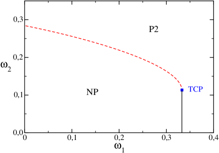
The diagram for $\omega_{3}=0$ ($K=2$) is shown in Fig. 3. For small values of $\omega_{2}$ we find a continuous transition, between the phases NP and P2, which ends at a tricritical point (TCP) located at $\omega_{1}^{TCP}=\frac{1}{(q-1)}$ and $\omega_{2}^{TCP}=\frac{1}{(q-1)^{2}}$, as found in ss07 . Above the tricritical point the transition becomes discontinuous. Here it is important to stress that this particular case ($\omega_{3}=0$) was studied in ss07 , considering distinguishable monomers and using the NIC method to find the coexistence lines. There three “stable“ phases were found: NP, P and DO, however, here (using the free energies) we find only two stable phases: NP and P2. Indeed, the DO fixed point is stable in a region of the parameter space, but the corresponding phase is never the one with the lowest free energy, that is, its free energy is always greater than that of the phases P2 or NP. In the same way, the TO phase is never the most stable in any region of the phase diagram, although, if we use the NIC method it appears to be stable for small values of $\omega_{1}$ and $\omega_{2}$ and large $\omega_{3}$. A detailed discussion of this point may be found the appendix A.

Figure 4: (Color online) Phase diagram for $\omega_{2}=0$. The dashed curve located left of the critical endpoint (CEP) (red) is a coexistence line between the phases NP and P2, and at the dashed curve right of the CEP (violet) phases P1 and P2 coexist. These two phases become indistinguishable at the critical point (CP) represented by a (purple) circle. Phases NP and P1 are separated by a continuous transition, represented by the (black) full line. This line meets the coexistence line at a critical endpoint (CEP), represented by a (green) square.

Figure 5: (Color online) Phase diagrams for: a) $\omega_{1}=0$, b) $\omega_{1}=1/3$ and c) $\omega_{1}=0.40$. The dashed curves are discontinuous transitions between phases NP and P2 (red) in a) and phases P1 and P2 (violet) in c). At the dotted line in c) the densities shown in Fig. 6 were calculated.

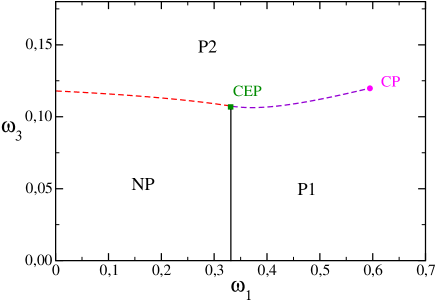
In the $\omega_{2}=0$ plane, we found a very rich phase diagram, as is shown in Fig. 4 For $\omega_{1}<\frac{1}{(q-1)}$ we find a first order transition between the phases NP and P2. At $\omega_{1}=\frac{1}{(q-1)}$, there is a continuous transition line between the phases NP em P1, this critical line ends at a critical endpoint (CEP). In the $\omega_{1}>\frac{1}{(q-1)}$ region we have a discontinuous transition between the phases P1 and P2 and this coexistence line ends at a critical point (CP).

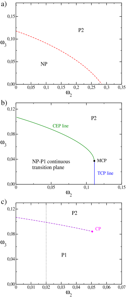
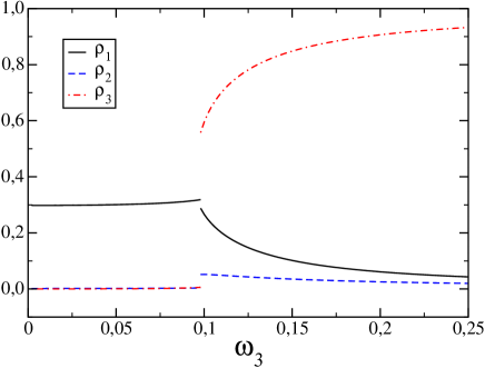
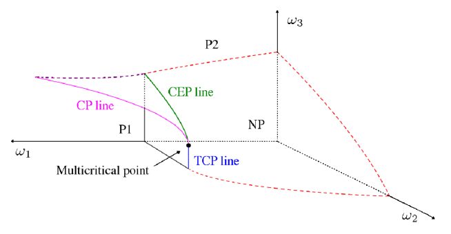
In Fig. 5, we show several diagrams, in the ($\omega_{2},\omega_{3}$) space, for different values of $\omega_{1}$. For $\omega_{1}=0$ (a) there is only a single coexistence line between the NP and P2 phases. Similar diagrams are obtained for all $\omega_{1}<\frac{1}{(q-1)}$. For $\omega_{1}=\frac{1}{(q-1)}$ (b) we have a critical surface (continuous transition) separating the NP and P1 phases. This surface is limited by a critical endpoint line and a tricritical line, and these two lines meet at a multicritical point (MCP). The multicritical point is located at $\omega_{1}^{MCP}=\frac{1}{(q-1)}$, $\omega_{2}^{MCP}=\frac{1}{(q-1)^{2}}$ and $\omega_{3}^{MCP}=\frac{1}{(q-1)^{3}}$, its location is determined in the appendix B. The tricritical point line lies at constant $\omega_{1}=\omega_{1}^{MCP}$ and $\omega_{2}=\omega_{2}^{MCP}$, and $0\leq\omega_{3}\leq\omega_{3}^{MCP}$. For $\omega_{1}>\frac{1}{(q-1)}$ (c) we have a discontinuous transition between the phases P1 and P2 and this coexistence surface ends at a critical line. The critical line starts at the multicritical point and the value of $\omega_{2}$ at the line decreases as $\omega_{1}$ and $\omega_{3}$ increase, so that the P1-P2 coexistence surface ends at $\omega_{1}=0.608762(1)$, $\omega_{2}=0$ and $\omega_{3}=0.121132(1)$. Also, to illustrate the discussion of the differences in both regular polymerized phases, we show in Fig. 6 the fixed point values of the densities as functions of $\omega_{3}$ for $\omega_{1}=0.4$ and $\omega_{2}=0.02$ (dashed line in phase diagram c) in Fig. 5).

Figure 6: (Color online)Densities as functions of $\omega_{3}$ for $\omega_{1}=0.4$ and $\omega_{2}=0.02$. Notice values at the coexistence of phases P1 and P2.

A sketch of the whole three-dimensional phase diagram is shown in Fig. 7 and this summarizes all the features discussed in the two-dimensional cuts of the phase diagram presented above.

Figure 7: (Color online) Sketch of the three-dimensional phase diagram. The first order transition surfaces: NP-P2 (red) and P1-P2 (violet), limited by dashed lines, are shown.

IV Comparison with the canonical simulations

The $K=3$ version of the model were originally studied by Krawczyk et al. kpor06 using Monte Carlo simulations. The simulations were performed considering a chain of constant size placed on an infinite lattice, so that they are in the canonical ensemble. To compare our grand-canonical results with the simulations we have to map our phase diagram to the canonical one. In this particular case, the usual procedure does not work because in the canonical simulation, as well as in experiments with diluted chains in a solvent, the canonical system is not homogeneous, but is composed by isolated chains in an excess of solvent (empty lattice sites). Therefore, we may say that in the simulations the polymer coexists with the empty lattice, namely, we have two phases coexisting: one of them polymerized (the polymer itself and the empty lattice sites close to it) and a non-polymerized (the remaining empty lattice sites). It follows that in our grand-canonical calculations the canonical situation of the simulations corresponds to the critical and coexistence surfaces limiting the NP phase, and the critical lines and points at these surfaces must be the critical lines in the canonical diagram.

In the canonical simulations, Krawczyk et al. fixed the energy of a single monomer to be equal to zero, i. e., the Boltzmann weight $e^{\beta_{0}}=1$. The parameters in the simulations were $\beta_{\ell}=-\beta\varepsilon_{\ell}$, with $\ell=1,2$, where $\beta=1/k_{B}T$ and $\varepsilon_{\ell}$ is the energy associated with sites occupied by $\ell+1$ monomers. To relate the simulational parameters to the ones used in our grand-canonical calculations, we notice that in our calculations the statistical weight of a site occupied by a single monomer is $\omega_{1}=z$, where $z$ is the activity of a monomer. A energy $\varepsilon_{1}$ is associated to a site with two monomers, thus the corresponding statistical weight is $\omega_{2}=z^{2}\,e^{-\beta\varepsilon_{1}}$ and for a site with three monomers, we have $\omega_{3}=z^{3}\,e^{-\beta\varepsilon_{2}}$. Therefore, the parameters used in the canonical simulations relate to the parameters used here as

$$\beta_{1} = \ln{\left[\frac{\omega_{2}}{\omega_{1}^{2}}\right]},$$ (23a)

$$\beta_{2} = \ln{\left[\frac{\omega_{3}}{\omega_{1}^{3}}\right]}.$$ (23b)

Figure 8: (Color online) Canonical phase diagram. The curve at $\beta_{2}>0$ (green) is the CEP line and the straight line at $\beta_{2}<0$ (blue) is the tricritical line. The multicritical point, where the two lines meet, is located on the origin and represented by a circle.

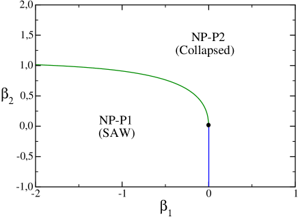
The canonical phase diagram which we found in the $\beta_{1},\beta_{2}$ parameters is shown in Fig. 8, for a Bethe lattice with $q=4$. The multicritical point is located on the origin. The tricritical line is placed at $\beta_{1}=0$ and $\beta_{2}$ ranging between $-\infty$ and $0$. The critical endpoint line is in the negative $\beta_{1}$ and positive $\beta_{2}$ quadrant. For $\beta_{1}<0$ and below the CEP curves, we have a region corresponding to the critical surface NP-P1 in the grand-canonical phase diagram. Thus, in this region the polymers are formed by chains with predominance of single visited sites, this is agreement with the simulations results. The other region corresponds to coexistence surface between NP and P2 phases, thus in this region sites with two or three monomers are more frequent, characterizing a “collapsed” phase. Indeed, a dense polymerized phase, in the grand-canonical ensemble, is characterized by the lattice completely occupied by monomers ($\rho=1$), and, in our solution method, this would appear as a fixed point with one or more diverging ratios $R_{i}$. In this model we do not find any collapsed phase in this sense, such a phase may be present in SASAW’s with attractive interactions between bonds in elementary squares on the square lattice sms96 . Nevertheless, as the density of the polymerized phases at the coexistence loci is nonzero, this already sets $\nu=1/d$ and therefore it is appropriate to call this a collapsed phase.

The location of the multicritical point in the Bethe lattice solution ($\beta_{1}=\beta_{2}=0$) is not physically reasonable because it corresponds to non-interacting monomers. We expect that the transition to the collapsed phase occurs in a attractive region for at least one of the parameters ($\beta_{1},\beta_{2}$), but for $\beta_{2}<0$ the transition line is along the $\beta_{2}$ axis ($\beta_{1}=0$) and this it is not reasonable. But, it is important to keep in mind that our solution is a mean-field approximation, which generally overestimates the domain of the ordered phase. Actually, this inconsistency was already noted in the solution of the case $K=2$ ss07 , and was one of the motivation to perform a calculation of this model on the Husimi lattice, which is expected to lead to results closer to the ones on regular lattices. This solution, which corresponds to the particular case $\omega_{3}=0$ and $\beta_{2}=-\infty$ of the model considered here, on the Husimi lattice build with squares (a second order approximation for the square lattice) displays a tricritical point located at $\omega_{1}=0.3325510(6)$ and $\omega_{2}=0.120544(4)$, which in the canonical variables corresponds to $\beta_{1}\approx 1.09$ and $\beta_{2}=-\infty$. Thus, within this (better) approximation, at least in $\beta_{2}=-\infty$ limit, we find the transition in the expected region ($\beta_{1}>0$). This suggests that the whole tricritical line may be at positive values of $\beta_{1}$, as found in the simulations, and therefore, the multicritical point may not be at the origin.

Finally, there is the question of the order of the transitions. In the simulations, Krawczyk et al. suggest, by estimating the fluctuations of the order parameter in their simulations, that for $\beta_{1}<0$ the transition is continuous and for $\beta_{2}<0$ it becomes of first-order one, and this lines match at a tricritical point. In our phase diagram, all transitions are continuous but we have a tricritical line in $\beta_{2}<0$ and a CEP line in $\beta_{1}<0$ region. Although both transitions are always continuous the critical exponents should be different in the two lines, due to the fact that the transitions are of a different nature (critical endpoints and tricritical points). Actually, since in the canonical conditions the tricritical line is always approached in the weak direction gw70 , that is, staying on the coexistence surface, the weak tricritical exponents will be found. In particular, in three dimensions, the tricritical exponents will be classical, apart from logarithmic corrections ls84 . In particular, as in the simulations Krawczyk et al. have estimated the fluctuations of order-parameter like variables, for the tricritical line the expected exponent would be $\gamma=2$. The critical endpoint line, however, is characterized by regular critical exponents, and estimates of $\gamma$ for the polymerization transition in three dimensions are around $1.158$ g00 , while the classical value is equal to unity. The estimates from the simulations have lead Krawczyk et al. to suggest that the transition line which corresponds to the tricritical line in our approximate calculations should be of first order. They also remark that this transition appears to be stronger than the one which corresponds to our critical endpoint line. It remains an open question if the stronger singularity observed in the former transition could not be due to the larger exponent for the singularity in the fluctuations of the order parameter.

V Final discussions and conclusion

Although, as discussed above, there are some differences between the canonical simulational estimates and our present Bethe lattice calculations, they have many similarities. It is worth mentioning that in the simulations no transitions were found for the RF model on the square lattice kpor06 . It is possible that actually the model shows a qualitatively different behavior on two-dimensional lattices than the one found here, since the Bethe lattice may be regarded as an infinite dimensional lattice b82 .

Another question which is worth to be considered is the relation of the model with multiple monomers per site with the problem of the collapse transition for polymers in a poor solvent. As mentioned above, one of the simplest models used to study these transition is the SASAW’s model, so that it is interesting to find a relation between both models. We may notice that the real situation of a polymer in a poor solvent may be discretized by supposing the volume to be composed by cells of roughly the size of a monomer, so that each cell will be either occupied by a monomer (full) or by a solvent molecule (empty). For simplicity, we are assuming the solvent molecules to have roughly the same size as the monomers. Now if we require the cells to form a regular lattice, we end up with a lattice gas model. The monomer-monomer, monomer-solvent and solvent-solvent interactions may then be considered effectively by introducing an attractive interaction between monomers in first-neighbor sites which are not connected by a polymer bond. Now we could imagine larger cells, composed by $K$ of the original cells, so that each of them may be occupied by up to $K$ monomers. If we now add the constraint that no polymer bond may be formed between monomers in the same cell and that attractive interactions only between monomers in the same cell will be considered we end up essentially with the MMS model. The parameters in the grand-canonical SASAW’s models are the activity of a monomer $z$ and the attractive interaction $-\epsilon$ ($\epsilon>0$) between monomers. Considering the correspondence of this model with the MMS model, we notice that the total contribution of a site with $i$ monomers to the internal energy will be $-\epsilon\,i(i-1)/2$, so that we may relate the parameters of both models as follows:

$$\omega_{i}=z^{i}\omega^{e(i)},i=1,2,\ldots,K,$$ (24)

where the exponent $e(i)=i(i-1)/2$ and $\omega=exp(-\epsilon/k_{B}T)$. Therefore, we notice that the MMS model with up to $K$ monomers per site corresponds to a grand-canonical SASAW’s model with constraints in a two-dimensional subspace of its original $K$-dimensional parameter space. If we consider the canonical situation, the dimensionality of the parameter space is reduced by one in both models.

In the particular case of the $K=3$ MMS model, we have the relations $\omega_{1}=z$, $\omega_{2}=z^{2}\omega$, and $\omega_{3}=z^{3}\omega^{3}$. Thus, recalling the definitions of the canonical parameters $\beta_{i}$ of the model Eq. (23), it will correspond to the canonical SASAW’s model with constraints for $\beta_{2}=3\beta_{1}$. For the Bethe lattice solution presented here, the multicritical point is located at the origin in the $(\beta_{1},\beta_{2})$ space, and this point belongs to the SASAW’s subspace. However, as discussed above, this unphysical localization of the multicritical point may be due to the approximate character of the solution. In the simulations by Krawczyk et al. of the RF model on the cubic lattice the multicritical point is located in the first quadrant of the $(\beta_{1},\beta_{2})$ space (Fig. 2 of reference kpor06 ). Unfortunately the precision in the estimated location of the multicritical point in the simulations seems not to be sufficient to determine its situation with respect to the $\beta_{2}=3\beta_{1}$ line. It would be very interesting to find out if the multicritical point is located above the SASAW’s line, in which case the collapse transition can be identified with the point where the line crosses the tricritical line of the MMS model. In this case, the collapse transition in the MMS model would be a tricritical point, which is consistent with the well established result for this transition.

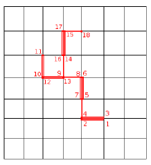
Finally, we notice that we have not studied the RA model here, where immediate reversals are allowed. In the simulations of the $K=3$ case of this model on the cubic lattice, no transition to the collapsed phase was found kpor06 , suggesting that the RF constraint is essential to produce this transition. One possible explanation of the reason for the effect of the RF constraint on the MMS model is that without this constraint contributions are possible that actually correspond to extended chainlike structures. Let us illustrate this by an example for the $K=2$ model on a square lattice. If we have $\omega_{2}\gg\omega_{1}$, beside the DO phase, where a pair of parallel bonds starts on the surface and crosses the lattice, if immediate reversals are allowed other chainlike structures, with a much higher entropy, are possible with double occupied sites only, as may be seen in Fig.9. Such a contribution has an exponent $\nu$ which correspond to extended polymers, and if these contributions dominate in the polymerized phase no extended-collapsed transition will occur. Of course, this argument is speculative and should be verified by simulations or approximate calculations for the RA model. As a final remark, we notice that no transition was found in the simulations of the $K=3$ model on the square lattice kpor06 . Although mean-field like calculations such as the one presented here become less reliable as the dimension is lowered, thus making it possible that e transition found in those approximations is actually absent in the two-dimensional case, it is worth remaining that the model of SASAW’s on the square lattice is well studied and shows a tricritical collapse transition ds85 , and therefore it is interesting to further investigate the MMS model on two-dimensional lattices.

Figure 9: (Color online) Contribution for the $K=2$ RA model on a square lattice, with a chainlike structure where all sites visited by the polymer are occupied by two monomers. The numbers correspond to the sequence of monomers in the chain.

Appendix A Coexistence surfaces in Bethe lattice calculations

The determination of the coexistence loci for solutions on hierarchical lattices such as the Bethe and Husimi lattices presents some difficulties, which may be related to the fact that in such lattices one may readily obtain mean values in the central region, but it is not straightforward to obtain the free energy (particularly the entropy) as a mean value. One possibility is to integrate the state equations to obtain the free energy, this may be even performed analytically for some simple models such as the Ising model b82 . In other cases it is possible to perform the integration numerically, using a Maxwell construction to locate the discontinuous transition. A detailed discussion of this point was presented by Pretti p03 , analyzing particularly the proposals of Gujrati to obtain the bulk free energy which was presented above g95 and the one of Monroe, based on the Jacobian of the recursion relations at the fixed point m94 . Also, a simple recursive criterion was used to find the coexistence locus for a model of SASAW’s on the Husimi lattice, which consists in iterating the recursion relations imposing ‘natural’ initial conditions on the ratios. In the region of the parameter space where the coexistence locus is located, there are at least two stable fixed points, and the coexistence surface is proposed to be the boundary of the basins of attraction of the fixed points when the iteration is started with the ‘natural’ initial conditions. In the previous studies of the MMS model on Bethe and Husimi lattices, the recursive procedure was used, but as shown above it lead to results which are even qualitatively different from the ones obtained using the more controlled approach by Gujrati. Here we will discuss these questions for a simpler model than the one above: SASAW’s on the Bethe lattice, which was studied some time ago ss90 .

The model is defined in the grand-canonical ensemble, so that $z$ will be the activity of a monomer incorporated in the chains. The endpoints of the chains are constrained to be on the surface of the tree. A Boltzmann factor $\omega>1$ is associated to each pair of monomers in first neighbor sites of the tree which are not connected by a polymer bond, to take care of the attractive interactions. As usual, we define partial partition functions for subtrees. The subtrees have a edge at the root which is connected to the root site, to which $q-1$ subtrees of the previous generation are attached. We call $g_{0}$ the partial partition functions for a subtree with no monomer on its root site, $g_{1}$ will be the partial partition functions for a tree with a monomer on the root site and no bond on the root edge, while $g_{2}$ stands for the partial partition functions of a subtree with a monomer on the root site and a bond on the root edge. The recursion relations for these partial partition functions are easily found to be:

$$g^{\prime}_{0}\, = \,(\,g_{0}\,+\,g_{1}\,)^{q-1},$$ (25a)

$$g^{\prime}_{1}\, = \,\binom{q-1}{2}\,z\,g_{2}^{2}\,(g_{0}+\omega\,g_{1})^{q-3}\,,$$ (25b)

$$g^{\prime}_{2}\, = \,(q-1)\,z\,g_{2}(g_{0}+\omega\,g_{1})^{q-2},$$ (25c)

Proceeding as usual, we may define the ratios $R_{1}=g_{1}/g_{0}$ and $R_{2}=g_{2}/g_{0}$, and the recursion relations for them are:

$$R^{\prime}_{1}\, = \,\binom{q-1}{2}\,z\,R_{2}^{2}\,\frac{(1+w\,R_{1})^{q-3}}{(1+R_{1})^{q-1}}.$$ (26a)

$$R^{\prime}_{2}\, = \,(q-1)\,z\,R_{2}\,\frac{(1+w\,R_{1})^{q-2}}{(1+R_{1})^{q-1}},$$ (26b)

We should remark that the model was defined in a different but equivalent way in the earlier calculation ss90 , where an activity $x$ was associated to each bond of the chains. Since all chains are long, as they are constrained to start at the surface of the tree, these two formulations are equivalent. For example, the recursion relations (3.8) in this reference correspond to the ones presented here if we relate the ratios used in both calculations as $A=\sqrt{z}R_{2}$ and $B=R_{1}$, with $x=(q-1)z$.

The partition function of the model on the Cayley tree may be obtained if we consider the operation of attaching $q$ subtrees to the central site of the lattice:

$$Y\,=\,(g_{0}+g_{1})^{q}+\binom{q}{2}\,z\,g_{2}^{2}\,(g_{0}+\omega g_{1})^{q-2},$$ (27)

and, following Gujrati’s prescription Eq. (22), the reduced bulk free energy per site is

$$\phi_{b}\,=\,-\frac{1}{2}\left\{q\ln{(1+R_{1}^{*})^{q-1}}-(q-2)\,\ln\left[(1+R_{1}^{*})^{q}+\binom{q}{2}zR_{2}^{*2}(1+\omega R_{1}^{*})^{q-2}\right]\right\},$$ (28)

where $(R_{1}^{*},R_{2}^{*})$ correspond to a fixed point values of the recursion relations Eqs.(26).

Non-polymerized fixed point

In the non-polymerized phase we have $R^{NP}_{1}\,=\,0$ and $R^{NP}_{2}\,=\,0$, the eigenvalues of the Jacobian are:

$$\lambda_{1}\,=\,\left.\frac{\partial\,R^{\prime}_{2}}{\partial\,R_{2}}\right|_{NP}\,=\,(q-1)\,z\;\;\;;\;\;\;\lambda_{2}\,=\,\left.\frac{\partial\,R^{\prime}_{1}}{\partial\,R_{1}}\right|_{NP}\,=\,0.$$ (29)

Therefore, the stability limit of the non-polymerized fixed point will be $z_{sl}^{NP}=1/(q-1)$. Using Eq.(28) we see the free energy vanishes for this phase, $\phi_{b}^{NP}=0$, as expected.

Polymerized fixed point

In this phase $R_{i}^{P}\neq 0$, and $R_{1}^{P}$ can be obtained from Eq. (26b), which in this case takes the form

$$(1+R_{1}^{P})^{q-1}\,-\,(q-1)\,z\,(1+\omega\,R_{1}^{P})^{q-2}\,=\,0\,.$$ (30)

For the particular case $q=3$ the fixed point equation above is quadratic, and a simple expression may be found for the fixed point value of $R_{1}$:

$$R_{1}^{P}=\omega z-1+\sqrt{(\omega z-1)^{2}-1+2z}.$$ (31)

The other root of the equation corresponds to an unstable fixed point. Once $R_{1}^{P}$ is obtained, $R_{2}^{P}$ may be found using the other fixed point equation, related to the recursion relation Eq. (26a), and is given by

$$(R_{2}^{P})^{2}\,=\,\frac{2}{q-2}\,R_{1}^{P}\,(1+\omega\,R_{1}^{P})\,.$$ (32)

The stability limit of this phase may be found by requiring the largest eigenvalue of the Jacobian of the recursion relations Eqs. 26 to be equal to one. In general, the equation defining this limit of stability has to be solved numerically, but for $q=3$ it is simple to find the result:

$$z_{SL}^{P} = \frac{1}{2},\;\;\mbox{for $\omega<2$,}$$ (33a)

$$z_{SL}^{P} = \frac{2(\omega-1)}{\omega^{2}},\;\;\mbox{otherwise.}$$ (33b)

The tricritical point is obtained as the point on the critical line $x=1/(q-1)$ where $R_{1}=0$ is a double root of Eq.(30):

$$z_{TC}\,=\,\frac{1}{q-1}\;\;\;\omega_{TC}\,=\,\frac{q-1}{q-2}$$ (34)

The first-order line

For $\omega>\omega_{TC}$ the first-order transition line can be obtained using the condition $\phi_{b}^{P}(x,\omega)\,=\,\phi_{b}^{NP}=0$, which gives

$$(1\,+\,R_{1}^{P})^{2\,(q-1)}\,=\,\left[1\,+\,R_{1}^{P}\,+\,\frac{q}{q-2}\,(1\,+\,\omega\,R_{1}^{P})\,R_{1}^{P}\right]^{q-2},$$ (35)

In general, this equation has to be solved numerically, but for $q=3$ it is straightforward to obtain an analytical solution, which is:

$$R_{1}^{FO}\,=\,\sqrt{3\,\omega-2}\,-\,2\;,$$ (36)

and, from Eq. (31) we obtain,

$$z^{FO}(\omega)\,=\,\frac{(\sqrt{3\,\omega-2}\,-\,1)^{2}}{2(\omega\,\sqrt{3\,\omega-2}\,-\,2\,\omega+1)}\;\;\;;\omega\,\geq\omega_{TC}\,=\,2.$$ (37)

The first order line calculated above does coincide with the one obtained in the earlier calculation ss90 using the equal area rule. This is expected, since the densities of monomers and of interactions in the central region of the Cayley tree, calculated directly from the partition function Eq. (27) are equal to the ones obtained from the bulk free energy per site Eq. (28). Let us now consider the iterative prescription suggested by Pretti in p02 . One iterates the recursion relations Eqs. (26) starting with ‘natural’ initial conditions for the partial partition functions $g_{0}^{(0)}=1$, $g_{1}^{(0)}=0$, and $g_{2}^{(0)}=z$, so that the initial values for the ratios are $R_{1}^{(0)}=0$ and $R_{2}^{(0)}=z$. One then estimates the coexistence line to be at the point in the $(z,\omega)$ parameter space where the fixed point reached iterating the recursion relations switches between the non-polymerized and polymerized phases. The results of all calculations for a lattice with $q=3$ are displayed in the phase diagram in Fig. 10. The NIC method leads to a first order line which is clearly different from the one obtained using the bulk free energy. Actually, in more complex models, the ‘natural’ initial conditions may not be unique, and different choices for them could lead to different results for the coexistence locus. The other methods to define the coexistence locus are defined solely by the recursion relations and the partition function. Also, despite the intuitive physical appeal of the method, its justification based on more solid arguments is still lacking.

Figure 10: (Color online) Phase diagram for SASAW’s on a Bethe lattice with coordination $q=3$. Full (black) line is a continuous polymerization transition. Dotted lines are the limits of stability of the non-polymerized (right) and polymerized (left) phases. The dashed (red) line is the coexistence locus between both phases obtained from the free energy, while the dash-dotted (blue) line is the coexistence locus estimated using the recursive procedure.

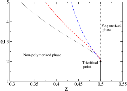
Although in the SASAW’s model discussed here the iterative procedure has lead only to a quantitative error in the location of the first order line, qualitative differences can result in more involved models. An example is the MMS model. The DO and TO fixed points, do not appear in the phase diagram despite the fact that the fixed points associated to them are actually stable in regions of the parameter space. This is due to the fact that the free energy of the P1 and P2 phases is smaller in those regions. If, however, the iterative procedure is used, this will be no longer the case and those phases actually appear in the phase diagram, as may be seen in the particular case $\omega_{3}=0$ in reference ss07 . For $K=3$ both DO and TO phases appear in the phase diagram if the recursive procedure is used.

Finally, we will briefly discuss the suggestion by Monroe m94 that at the coexistence the leading eigenvalues of the Jacobian of both phases should be equal. We may consider points on the coexistence line Eq. (37) for $q=3$. If the eigenvalue which corresponds to the polymerized phase would be equal do the one associated to the non-polymerized phase $\lambda_{NP}=2z$, then the expression:

$$\Delta=(J_{1,1}-2z)(J_{22}-2z)-J_{1,2}J_{2,1},$$ (38)

where $J_{i,j}$ are the elements of the Jacobian calculated at the polymerized fixed point, should vanish on the coexistence line. It may be shown that this expression does not vanish for $\omega>2$, thus showing that the Monroe criterium is not equivalent to the free-energy criterium for this particular model. It is interesting to remark that in other models this equivalence was found p03 .

Appendix B Location of the multicritical point

To find the location of the multicritical point in the parameter space of the model, we look for higher order roots with vanishing ratios of the fixed point equations which follow if we set $R^{\prime}_{i}=R_{i}$ in the recursion relations Eqs. 6. An inspection of the fixed point equations suggests the following ansatz for the ratios close to the non-polymerized fixed point: $R_{2}=aR_{1}^{2}$ and $R_{3}=bR_{1}^{3}$. We then substitute these leading order terms into the fixed point equations and require them to be satisfied up to order 4 in $R_{1}$. This furnishes five equations: from the first recursion relation Eq. (6a) we get one equation for order $R_{1}$ and another for order $R_{1}^{2}$. The second recursion relation Eq. (6b) furnishes two equations, one for order $R_{1}^{2}$ and the other for order $R_{1}^{4}$. Finally, recursion relation Eq. (6c) provides an additional equation for order $R_{1}^{3}$. In the sequence adopted above, the equations are:

$$1 = (q-1)\omega_{1},$$ (39a)

$$\binom{q-1}{2}\,\omega_{1} = 3\,\binom{q-1}{3}\,\omega_{2}+4\,\binom{q-1}{2}\,\omega_{2}a,$$ (39b)

$$a = \binom{q-1}{2}\,\omega_{2}+(q-1)\omega_{2}a,$$ (39c)

$$\binom{q-1}{2}\,\omega_{1}a = 6\,\binom{q-1}{4}\,\omega_{3}+15\,\binom{q-1}{3}\,\omega_{3}a+4\,\binom{q-1}{2}\,\omega_{3}a^{2}+$$ (39d)

$$6\,\binom{q-1}{2}\,\omega_{3}b,$$

$$b = \binom{q-1}{3}\,\omega_{3}+2\,\binom{q-1}{2}\,\omega_{3}a+(q-1)\omega_{3}b.$$ (39e)

These equations may easily be solved, leading to $\omega_{1}=1/(q-1)$, $\omega_{2}=1/(q-1)^{2}$, $\omega_{3}=1/(q-1)^{3}$, $a=1/2$, and $b=1/6$. The behavior of the ratios in the vicinity of the multicritical point has been verified numerically.

References

- (1) P. J. Flory, Principles of Polymer Chemistry, edition, Cornell University Press, NY (1966).
- (2) P. G. de Gennes, Phys. Lett. A 38,339 (1972).
- (3) P. G. de Gennes, Scaling Concepts in Polymer Physics, Cornell University Press, NY (1979).
- (4) P. G. de Gennes, J. Physique Lettres 36, 1049 (1975).
- (5) B. Derrida and H. Saleur, J. Phys. A 18, L1075 (1985); H. Saleur, J. Stat. Phys. 45, 419 (1986).
- (6) B. Duplantier and H. Saleur, Phys. Rev. Lett 59, 539 (1987); B. Duplantier, Phys. Rev. A 38, 3647 (1988).
- (7) J. F. Stilck, K. D. Machado, and P. Serra, Phys. Rev. Lett. 76, 2734 (1996); J. F. Stilck, P. Serra, and K. D. Machado, Phys. Rev. Lett. 89, 169602 (2002); P. Serra, J. F. Stilck, W. L. Cavalcanti, and K. D. Machado, J. Phys. A 37, 8811 (2004);K. D. Machado, M. J. de Oliveira, and J. F. Stilck, Phys. Rev. E 64, 051810 (2001); D. P. Foster, J. Phys A 40, 1963 (2007).
- (8) M. Pretti, Phys. Rev. Lett. 89, 169601 (2002).
- (9) J. Krawczyk, T. Prellberg, A. L. Owczarek, and A. Rechnitzer, Phys Rev. Lett. 96, 240603 (2006).
- (10) C. Domb and G. S. Joyce, J. Phys. C 5, 956 (1972).
- (11) P. Serra and J. F. Stilck, Phys. Rev. E 75, 011130 (2007).
- (12) T. J. Oliveira, J. F. Stilck, and P. Serra Phys. Rev. E 77, 041103 (2008).
- (13) P. D. Gujrati, Phys. Rev. Lett. 74, 809 (1995).
- (14) R. B. Griffiths and J. C. Wheeler, Phys. Rev. A 2, 1047 (1970); R. B. Griffiths, Phys. Rev. B7, 545 (1973).
- (15) I. D. Lawrie and S. Sarbach in Phase Transitions and Critical Phenomena, vol. 9, ed. by C. Domb and J. L. Lebowitz, Academic Press (1984).
- (16) D. MacDonald et al, J. Phys. A 33, 5973 (2000).
- (17) R. J. Baxter, Exactly Solved Models in Statistical Mechanics, Academic, London (1982).
- (18) M. Pretti, J. Stat. Phys. 111, 993 (2003).
- (19) J. L. Monroe, Phys. Lett A 188, 80 (1994).
- (20) P. Serra and J. F. Stilck, J. Phys. A 23, 5351 (1990).