The Non-Linear Fisher Information content of cosmic shear surveys

Abstract

We quantify the Fisher information content of the cosmic shear survey two-point function as a function of noise and resolution. The two point information of dark matter saturates at the trans-linear scale. We investigate the impact of non-linear non-Gaussianity on the information content for lensing, which probes the same dark matter. To do so we heavily utilize N-body simulations in order to probe accurately the non-linear regime. While we find that even in a perfect survey, there is no clear saturation scale, we observe that non-linear growth induced non-Gaussianity could lead to a factor of  4 reduction for the common Dark Energy figure of merit. This effect is however mitigated by realistic levels of shot noise and we find that for future surveys, the effect is closer to a factor of 1.5. To do so, we develop a new scheme to compute the relevant covariant matrix. It leads us to claim an unbiased estimator with an order of magnitude improvement in accuracy with only twice more simulations than previously used. Finally, we evaluate the error on the errors using bootstrap methods.

I Introduction

What is the information content of cosmic shear surveys? Although this question has been addressed many times given the current interest in cosmic shear surveys, to answer it accurately turns out to be a non-trivial task. It is the purpose of this work to offer one answer to this question.

The measure of cosmic shear (e.g. Bartelmann and Schneider (2001); Van Waerbeke and Mellier (2003) for reviews), is considered to be one of the most promising observational tools to understand the origin of the accelerating expansion of the universe Albrecht et al. (2006). Commonly attributed to the existence of some extra unknown physics loosely labelled Dark Energy (DE), its exact nature became one of the salient questions in contemporary cosmology Riess et al. (2004); Astier et al. (2006); Eisenstein et al. (2005); Cole et al. (2005); Tegmark et al. (2006); Komatsu et al. (2008); Kilbinger et al. (2008). Characterising the physical properties of DE is the main scientific driver for the development of new and very ambitious surveys.

Our work was motivated by recent investigations of the information content of the 3D matter power spectrum as quantified by the projection of the Fisher information on the amplitude Rimes and Hamilton (2005, 2006); Hamilton et al. (2006); Neyrinck et al. (2006). Quantifying the information through this well defined statistic (insightful even if restrictive), the answer obtained in these papers was somewhat surprising. While a Gaussian like behavior was observed on linear (large) scales, the non-linear growth of structures entails an information saturation at mildly non-linear scales. A quasi-Gaussian behavior was recovered once fully in the non-linear regime but at a substantially lower level. When devising a survey, it means that optimizing the survey to gain sensitivity and resolution in the trans-linear regime (where the power spectrum is currently interpreted cosmologically), would not entail much pay-off if one were focusing on this statistic only. Despite the fact that the effect of the non-linear growth of structures had been widely studied before these works, formulating it this way led to this surprising answer, heuristically understood within the context of the halo model Neyrinck et al. (2006). Neyrinck and Szapudi (2007) later showed that if we project the Fisher information into other parameters, analogous behavior are then observed. This validates the insightful value of the amplitude projection. As a consequence, for the sake of simplicity, we will loosely call information the projection of the Fisher information onto various subspaces (amplitude or DE statistics). And although we will define all our statistics precisely, their label as information is definitely restrictive. We will look at them as a way to highlight the departure from the Gaussian behavior usually assumed when forecasting the constraining power of those survey. Beyond this departure, to quantify fully the information content in the non-Gaussian regime is a task we will not endeavor in this paper. This paper explores the variance of the power spectrum, which is a 4-point statistic of the density field, and its variance, which is an 8-point statistic. Potentially, higher order estimators, e.g. 3 or 4 points functions, could contain additional information for non-Gaussian fields. The calculation of those errors, and errors on errors, is substantially more challenging. Early investigations Pen et al. (2003) indicated that those errors grow rapidly, making their use challenging.

Whereas new cosmic shear surveys are being advocated Albrecht et al. (2006) and designed Amara and Refregier (2007), we want to study in this work how this 3D information saturation translates into cosmic shear observables. In particular, one question we would like to answer is whether there exists a scale above which the Fisher Information for the two-point functions (projected onto the amplitude or the DE Figure of Merit) saturates. Since above a given angular scale ($\ell\geq 2000$), our lack of precise modeling of the physics of baryons might require enormous efforts to be addressed White (2004); Zhan and Knox (2004); Rudd et al. (2007), it would be interesting to know whether such a saturation happens and in particular how it compares to this theoretical uncertainty scale. To tackle this question will require to compute the cosmic shear error budget in the fully non-linear regime. While this questions has already been investigated in the literature White and Hu (2000); Cooray and Hu (2001); Semboloni et al. (2007); Takada and Jain (2008), we will address it using numerical N-body simulations to probe accurately the full non-linear regime (still neglecting baryons though), and a new way to build the covariance matrix from those quantities. This will lead us to an order improvement in accuracy as compared to previous numerical works in the literature. We will quantify this statement by measuring the errors on the errors using bootstrap techniques.

In this paper, we first begin by introducing the methodology of our work in Sec. II before revisiting the 3D matter power spectrum results in Sec. III as an introduction to the cosmic shear case developed in Sec. IV. We discuss in Sec. V the practical consequences of these results for current and coming optical surveys, as well as for CMB lensing.

II Methodology

If we want to infer a set of parameters $\alpha_{i}$ from observables $x$ of dimension $n_{x}$ following a multi-variate Gaussian distribution with a covariance matrix ${\bf C}\equiv$$\langle{\mbox{\boldmath$x$}}{\mbox{\boldmath$x$}}^{t}\rangle-\langle{\mbox{\boldmath$x$}}\rangle\langle{\mbox{\boldmath$x$}}\rangle$, the Fisher Information matrix is defined as Fisher (1936); Tegmark et al. (1997, 1998)

$${\bf F}_{ij}\equiv{1\over 2}{\rm tr}\left[{\bf C}^{-1}{\partial{\bf C}\over\partial\alpha_{i}}{\bf C}^{-1}{\partial{\bf C}\over\partial\alpha_{j}}\right]+{\partial\langle{\mbox{\boldmath$x$}}\rangle\over\partial\alpha_{i}}{\bf C}^{-1}{\partial\langle{\mbox{\boldmath$x$}}\rangle\over\partial\alpha_{j}}.$$ (1)

Its relevance for parameter estimation can be seen from the Cramér-Rao inequality stating that the Fisher matrix sets a lower bound on how well a parameter $\alpha_{i}$ can be measured, that is $\sigma^{2}(\alpha_{i})\geq 1/{\bf F}_{ii}$. We assume from now on that the covariance matrix ${\bf C}$ does not depend on $\alpha_{i}$ (for a discussion in the context of cosmic shear, see Eifler et al. (2008)) and, following Rimes and Hamilton (2005), we define the information content of $x$ as

$$Inf\equiv\sum_{ij}{\bf F}_{ij}=\sum_{ij}{\partial\langle{\mbox{\boldmath$x$}}\rangle\over\partial\alpha_{i}}{\bf C}^{-1}{\partial\langle{\mbox{\boldmath$x$}}\rangle\over\partial\alpha_{j}}.$$ (2)

In this paper, the observables we will consider will be either the 3D matter power spectra, ${\mbox{\boldmath$x$}}=P({\bf k})$, or the 2D convergence power spectra ${\mbox{\boldmath$x$}}=C_{\ell}^{\kappa}$ defined in Eq. 10. The parameters we will focus will be the standard cosmological parameters for a flat cosmological model whose density is dominated at late time by Dark Energy (DE) whose equation of state evolves as $w=w_{0}+w_{a}(1-a)$, $\alpha=(w_{0},w_{a},\omega_{m},\omega_{b},n_{s},\sigma_{8})$ Albrecht et al. (2006). The nominal value for those parameters correspond to the currently favored model, $\alpha=(1.,0.,0.1334,0.0228,0.963,0.796)$ Komatsu et al. (2008).

For pedagogical reasons, we will also consider a dimensionless version of Eq. 2

$$\bar{Inf}\equiv\sum_{ij}{\bf\bar{C}}_{ij}^{-1} ,\quad {\bf\bar{C}}_{ij}={\langle{\mbox{\boldmath$x$}}_{i}{\mbox{\boldmath$x$}}_{j}\rangle\over\langle{\mbox{\boldmath$x$}}_{i}\rangle\langle{\mbox{\boldmath$x$}}_{j}\rangle}.$$ (3)

This form would be obtained from Eq. 2 if we were measuring the amplitude of a template $P({\bf k})$ (or $C_{\ell}^{\kappa}$), so that the partial derivatives were unity. Note that because of non-linear effects, this amplitude does not correspond to $\sigma_{8}$ or the curvature perturbation amplitude $A_{S}$. To put it otherwise, what we will define as information in Sec. III and IV corresponds to the variance on the amplitude parameter, $\alpha$, if the observables were to be modeled as ${\mbox{\boldmath$x$}}=\alpha\bar{{\mbox{\boldmath$x$}}}$. We find this projection of the Fisher Information matrix onto this space to be a convenient quantity to visualize the property of this matrix. Given this definition, since we are interested in quantifying the effects on non-linearities on the information content of the measured convergence angular power spectrum (or matter power spectrum), it will be particularly insightful to investigate the scaling of $\bar{Inf}$ with a cut-off scale $\ell_{max}$ ($k_{max}$), that is the cumulative information content as function of the smallest (angular) modes measured. The comparison between the scaling on large scale (low $\ell$ and $k$) where the convergence (matter) field is expected to be Gaussian to the one in the non-linear regime (high $\ell$ and $k$) will thus be of particular relevance. For this purpose, we define in the matter power spectrum and angular power spectrum case (at wavenumber $k_{b}$ or multipole $\ell$),

$${\bf\bar{C}}_{k_{b}k_{b^{\prime}}<k_{max}}={\langle P_{k_{b}}P_{k_{b^{\prime}}}\rangle\over\langle P_{k_{b}}\rangle\langle P_{k_{b^{\prime}}}\rangle} \quad, \bar{Inf}(k_{max})=\sum_{k_{b},k_{b^{\prime}}<k_{max}}{\bf\bar{C}}_{k_{b}k_{b^{\prime}}}^{-1}\ ,$$ (4)

$${\bf\bar{C}}_{\ell_{1}\ell_{2}<\ell_{max}}={\langle C_{\ell_{1}}^{\kappa z_{1}z_{2}}C_{\ell_{2}}^{\kappa z_{3}z_{4}}\rangle\over\sqrt{\langle C_{\ell_{1}}^{\kappa z_{1}z_{1}}\rangle\langle C_{\ell_{1}}^{\kappa z_{2}z_{2}}\rangle\langle C_{\ell_{2}}^{\kappa z_{3}z_{3}}\rangle\langle C_{\ell_{2}}^{\kappa z_{4}z_{4}}\rangle}} \quad, \bar{Inf}(\ell_{max})=\sum_{\ell_{1},\ell_{2}<\ell_{max}}{\bf\bar{C}}_{\ell_{1}\ell_{2}}^{-1}\ .$$ (5)

The definition of $\bar{Inf}$ in Eq. 3 is particularly easy to interpret, since in the Gaussian case, where ${\bf C}_{ij}\propto$${\mbox{\boldmath$x$}}_{i}{\mbox{\boldmath$x$}}_{j}\delta_{ij}$, it directly reduces to half the number of measured modes. We thus have a simple analytical predictions for the expected scaling on large scales. Note that we choose to define $\bar{Inf}(\ell_{max})$ by imposing a sharp cut-off in Fourier space. An alternative definition consists in marginalizing over all the modes above $k_{max}$ ($\ell_{max}$) by adding a white noise level so that for example the signal to noise ratio equals 1 at $k=k_{max}$ ($\ell=$$\ell_{max}$). We checked that both approaches give equivalent results.

As visible from Eq. 3, the key quantities to evaluate the information content of our observables is the covariance matrix. For this purpose, we will use a Monte-Carlo approach and generate $n_{sim}$ realizations of the observables, ${\mbox{\boldmath$x$}}_{k}$, through N-body simulations including dark matter only. We make use of the publicly available CubePM code . CubePM is the successor to the particle-mesh N-body code PMFAST Merz et al. (2005) . In addition to the features provided by PMFAST – support for distributed memory systems through MPI and shared memory via OpenMP, minimal memory overhead and communications requirements – CubePM contains support for gas evolution through use of a TVD MHD module, particle-particle interactions at sub grid cell distances, optimal scaling up to (and hopefully beyond) 1000’s of nodes, as well as shared-memory parallelization via OpenMP to optimize memory usage on shared memory nodes.

Given a set of $n_{sim}$ realization for ${\mbox{\boldmath$x$}}_{k}$ that we write, ${\mbox{\boldmath$x$}}_{k}^{s=1,\ldots n_{sim}}$, we define as an estimator for ${\bf C}$ (see Hamilton et al. (2006) for a thorough discussion on how to measure ${\bf C}$ from one simulation only)

$${\bf\tilde{C}}_{ij} = {1\over n_{sim}}\sum_{s=1}^{n_{sim}}\left({\mbox{\boldmath$x$}}_{i}^{s}-\mu_{i}\right)\left({\mbox{\boldmath$x$}}_{j}^{s}-\mu_{j}\right),$$ (6)

$$\mu_{i} = {1\over n_{sim}}\sum_{s=1}^{n_{sim}}{\mbox{\boldmath$x$}}_{i}^{s}.$$ (7)

At this point, it is often missed that the inverse of a maximum-likelihood estimator for a variable $X$ is in general not an unbiased estimator of the inverse $X^{-1}$ Hartlap et al. (2006). To remedy this fact, a corrective factor is required. Since we also evaluate $\mu$ from our simulation, it can be shown that the following estimator for ${\bf C}^{-1}$ is unbiased:

$${\bf\hat{C}}^{-1} = {n_{sim}-n_{x}-2\over n_{sim}-1}{\bf\tilde{C}}^{-1}.$$ (8)

In the case we are interested in here, i.e. the the convergence angular (cross-) power spectrum covariance matrix $\langle C_{\ell_{1}}^{\kappa z_{1}z_{2}}C_{\ell_{2}}^{\kappa z_{3}z_{4}}\rangle$, we found that the number of independent modes, $n_{x}$, is not easy to define. Thus we dropped this corrective factor. We carefully checked the convergence of our results by increasing $n_{sim}$ (see Fig. 1 and Fig. 3).

Furthermore, to quantify the error on our statements, we will evaluate the errors on ${\bf\hat{C}}^{-1}$ by making use of the bootstrap method Efron and Tibshirani (1993). We will consider 1000 sets of $n_{sim}$ simulations randomly drawn from our $n_{sim}$ simulations and apply the above defined formalism to each. This procedure weighs in a random manner our initial set of N-body simulations. Even though it is unclear wether the number of independant realizations, i.e. simulations, we have is enough for the bootstrap method to be reliable it still gives us a valuable glimpse at the reliability of our statements, that is on the error on the error.

III Matter power spectrum information content

Figure 1: Cumulative information for the matter power spectrum at $z=1$ as defined in Eq. 4. We use either $n_{sim}=$ 50, 100, 200, 300 or 400 simulations. The bootstrap error bars are obtained using an analysis of 1000 sets of 400 simulations. The dashed orange line corresponds to the Gaussian prediction, i.e. the number of $k$ modes present in the simulation below $k_{max}$. Although the convergence does not appear to be perfect, the difference between the measurement using 300 or 400 appear smaller than the error bars everywhere. As such we can trust the results obtained with 400 simulations. This plot reproduces the results of Rimes and Hamilton (2006).

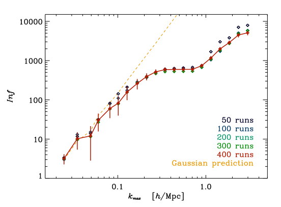
We first focus on the matter power spectrum and revisit the results of Rimes and Hamilton (2006). For this purpose, we ran 400 N-body simulations with their choice of cosmological model, that is a flat $\Lambda$CDM model with $\Omega_{m}=0.29$, $\Omega_{\Lambda}$=0.71, $\Omega_{b}=0.046$, $\sigma_{8}=0.97$ and $h$=0.71. Since we are interested in trans-linear scales, i.e. the transition regime between the fully linear regime and the fully non-linear regime, a comoving box size of 256 Mpc/$h$ with $256^{3}$ grid points is appropriate. This gives us roughly a mass resolution of 9.2$\times 10^{11}M_{\odot}$ and a force resolution of 1 Mpc/$h$. The initial conditions were generated at $z=200$.

To improve convergence, to increase the rank of ${\bf\tilde{C}}$ and to alleviate numerical issues when performing the inversion, we define $n_{x}=20$ bins logarithmically spaced in $k$ space and we measure the average power spectrum within a $k$ bin, ${\mbox{\boldmath$x$}}=P_{b}$ as

$${(2\pi)^{3}\over V_{box}}\langle\delta_{\bf k}\delta_{\bf k}^{*}\rangle_{{\bf k}\in b}=k_{b}^{3}P_{b}\ .$$ (9)

where $\delta_{k}$ is the Fourier transform of the matter over-density. We then make use of Eq. 4 and 8 with $n_{sim}=50,100$, $200$, $300$ or $400$ and $n_{x}=20$ to compute the cumulative information content for various $k_{max}$. The results at $z=1$ are plotted in Fig. 1 as well as the Gaussian prediction using the measured number of modes in the simulation, $\bar{Inf}^{G}(k_{max})=$$\sum_{b<k_{max}}(\#k\in b)$$\propto k_{max}^{3}$. Qualitatively similar results are obtained at different $z$.

First, we notice that the convergence in terms of the number of simulation used to compute $\bar{Inf}$ seems satisfying although not perfect. We estimate that the lack of convergence adds extra-uncertainties of the same order as the error we estimated using bootstraps. As discovered by Rimes and Hamilton (2006), the two remarkable features of this cumulative information are the following. Whereas on linear scales, say $k<$ 0.1 Mpc/$h$ the information content follows the scaling expected from a Gaussian random field, a sharp transition to a plateau is observed on trans-linear scales, and a return to a quasi-Gaussian scaling (but with a lower amplitude) in the fully non-linear regime. These features mean that the information, say on a primordial amplitude is conserved and could be measured with an accuracy directly proportional to (# modes)^-1/2 on linear scales, not much more is learned on trans-linear scales, i.e. the information is redundant with the one contained in linear scales. On the other hand, a quasi-Gaussian scaling is reestablished in the fully non-linear regime. The sharp transition from the linear to the non-linear regime can qualitatively be understood in the halo model framework, where it corresponds to the transition from the 2 halos term to the 1 halo term Neyrinck et al. (2006). Whereas on large scales, the information is contained in the 2 halos term and scales as the number of modes measured (or the number of halos in a given volume), on trans-linear scales, the 1 halo term starts to dominates but with a large variance since most of its contribution comes from rare massive halos. This large variance explains why it is hard to extract any information supplemental to the one obtained in the linear regime from this regime. On smaller scales though, the 1 halo term contribution comes mostly from numerous smaller mass halos whose number is much more constant, i.e. fluctuates with much less variance, and the information scales again roughly with the number of modes probed.

Now that we have reproduced and introduced the key results regarding the 3D matter power spectrum we move to the original results of this paper, that is how this information saturation effect in the matter power spectrum translates into some integral of it, i.e. into the cosmic shear observables.

IV Cosmic shear information content

We now make use of $n_{sim}=300$ N-body simulations run with our nominal cosmology to investigate the information content of cosmic shear surveys. To quantify the information, we choose as our observable the convergence cross-power spectra between two redshift bins $z_{i}$ and $z_{j}$ that we defined as Bartelmann and Schneider (2001); Van Waerbeke and Mellier (2003)

$$\tilde{n}_{z_{i}}\tilde{n}_{z_{j}}C_{\kappa\ell}^{z_{i}z_{j}}=\int_{0}^{\infty}dz\ W^{z_{i}}(z)W^{z_{j}}(z){H(z)\over D^{2}(z)}P(\ell/D(z),z)\ ,$$ (10)

where $H(z)$ is the Hubble parameter, $D(z)$ is the angular diameter distance, $P(k,z)$ is the 3-dimensional matter power spectrum at redshift $z$. The lensing kernel is defined as

$$W^{z_{i}}(z) = {3\over 2}\Omega_{m}{H_{0}^{2}D(z)\over H(z)}(1+z)\int_{z}^{\infty}dz^{\prime}\ n_{z_{j}}(z^{\prime}){D_{LS}(z,z^{\prime})\over D(z^{\prime})}\ ,$$ (11)

$$\tilde{n}_{z_{i}} = \int_{0}^{\infty}dz\ n_{z_{i}}(z)\ .$$ (12)

where $D_{LS}(z,z^{\prime})$ is the angular diameter distance between $z$ and $z^{\prime}$, $n_{z_{i}}(z)$ is the galaxy distribution in redshift bin $i$ and $\tilde{n}_{z_{i}}$ is the total number of galaxies in this redshift bin.

In this section, for the sake of simplicity, we will consider a uniform galaxy distribution in $n_{z}=1,\ldots,4$ redshift bins of width $\Delta z=0.5$ and defined as $1.0<z<1.5$, $1.5<z<2.0$, $2.0<z<2.5$ and $2.5<z<3.0$. Each distribution is normalized to unity, i.e. $n_{z_{i}}=1/\Delta z$ and $\tilde{n}_{z_{i}}=1$. This choice is motivated by our interest in low redshift diffuse lensing of the diffuse radiation originating from the 21cm line emission of galaxies Lu and Pen (2008); Pen et al. (2008); Lu et al. (2009). We will consider more realistic galaxy distribution functions when discussing specific surveys in Sec. V. As discussed in a companion paper Lu et al. (2009), we found that simulations with a box size of 200 Mpc/$h$, a 1024³ grid, and 512³ particles are close to optimal for our needs. Each one of these simulations takes about 4.5 hours using 8 nodes (64 cores) on CITA’s Sunnyvale cluster. We checked that finite resolution effects do not affect the convergence power spectra up to $\ell\simeq 10000$ that will define the smaller angular scale we consider in this work. This box size corresponds roughly to an area of 56 square degrees. As a consequence, when considering the dimensionless cumulative information, the sum is performed for $\ell\geq 50$.

To compute the covariance matrix using $n_{sim}=300$ simulations we employ an original method that avoid the artifacts present in previous methods. The now standard approach to simulate cosmic shear has been pioneered in White and Hu (2000); Jain et al. (2000). It consists in ray-tracing through a light cone build out of a collection of N-body simulations outputs at various redshifts. This method has been widely tested and its limitations (angular resolution, periodicity, mass resolutions, etc.) quantified White and Hu (2000); Jain et al. (2000); Hamana et al. (2002); Hamana and Mellier (2001); Semboloni et al. (2007). It provides great reliability, e.g. to produce $\kappa$ maps in the observational regime of interest nowadays. However, it is important to notice that given our box length, from the observer at $z=0$ till the most distant lens plane at $z=3$, 24 boxes are required. As such, in principle, one could build only 12 fully independent light cones out of our $n_{sim}=300$, a number far from enough for our Monte-Carlo approach to compute ${\bf C}^{-1}$. A common fix consists in using the same simulations more than once in a given light cone after random translations and rotations of the original box. While it does increase the number of light cone realisations that can be generated with a given number of N-body simulations, it introduces spurious correlations – density field from a same simulation at different redshift are not independent – which are hard to control safely. In fact, from the Limber approximation we know that the combination of shifting, stacking and recycling will lead to the correct power spectra since it is a linear function of the density field at each redshift with random phases. But this does not hold anymore when considering covariance matrices. To remedy this problem, we follow an original approach described below.

The basic idea goes as follows. We first compute the covariance matrix of the convergence (cross-) power spectra for each output boxes combination by averaging over all the $n_{sim}$ sims. The final convergence matrix is then an appropriately weighted sum of the covariance matrices computed at each output redshift. More formally, this procedure can be written this way. To compute the convergence power spectra, for each output boxes at a given redshift $z_{s_{1}}$, we project on a randomly chosen side the over-density field, $\delta({\mbox{\boldmath$x$}},z_{s_{1}})$, Fourier transform it and measure its 2D power spectrum, $\tilde{\delta}_{2d}({\bf k},z_{s_{1}})$. After converting the comoving wavenumber $k$ to an angular multipole $\ell=kD(z_{s_{1}})$, we weight the power spectrum by the lensing kernel $W^{z_{s1}}$ to transform it into an angular convergence power spectra at $z_{s_{1}}$ and bin it in $n_{\ell}=12$ bins:

$$\hat{C}_{\ell}^{{z_{s1}},{z_{s2}}}=\langle\tilde{\kappa}^{z_{s1}}_{\ell^{\prime}}{\tilde{\kappa}}^{z_{s2}\,\star}_{\ell^{\prime}}\rangle_{\ell\pm\Delta\ell}\ ,$$ (13)

where the average is taken over the $N_{\ell}$ contributing to this band power, $\ell-\Delta\ell<\ell^{\prime}=kD(z_{s_{1}})<\ell+\Delta\ell$, where

$${\tilde{\kappa}}^{z_{s1}}_{\ell}=\sum_{i}\tilde{\delta}_{2d}(\ell=kD(z_{s_{1}}),z_{i})W^{z_{s1}}(z_{i})\ ,$$ (14)

and where $W^{z_{s1}}$ is the lensing kernel for each slices if the sources are distributed in band $z_{s1}$ and the sum over $i$ denotes a sum over outputted simulation boxes. It follows that to compute the convergence cross power spectra covariance matrix,

$$Cov\left(C_{\ell}^{{z_{s1}},{z_{s2}}},C_{\ell^{\prime}}^{{z_{s3}},{z_{s4}}}\right) = \langle{C_{\ell}^{{z_{s1}},{z_{s2}}}C_{\ell^{\prime}}^{{z_{s3}},{z_{s4}}}}\rangle-\langle{C_{\ell}^{{z_{s1}},{z_{s2}}}}\rangle\langle{C_{\ell^{\prime}}^{{z_{s3}},{z_{s4}}}}\rangle\quad,$$ (15)

we need to compute using our $n_{sim}$ simulations, both

$$\langle C_{\ell}^{{z_{s1}},{z_{s2}}}C_{\ell^{\prime}}^{{z_{s3}},{z_{s4}}\star}\rangle_{sim} = \langle{\tilde{\kappa}_{\ell}^{z_{s1}}{\tilde{\kappa}}_{\ell}^{z_{s2}\,\star}(\tilde{\kappa}_{\ell^{\prime}}^{z_{s3}}{\tilde{\kappa}}_{\ell^{\prime}}^{z_{s4}\,\star})^{\star}}\rangle_{sim}$$

$$= \sum_{i_{1},i_{2},i_{3},i_{4}}W^{z_{s1}}(z_{i_{1}})W^{z_{s2}}(z_{i_{2}})W^{z_{s3}}(z_{i_{3}})W^{z_{s4}}(z_{i_{4}})\langle{\tilde{\delta}_{2d}(\ell,z_{i_{1}}){\tilde{\delta}_{2d}}^{\star}(\ell,z_{i_{2}})\tilde{\delta}_{2d}^{\star}(\ell^{\prime},z_{i_{3}}){\tilde{\delta}_{2d}}(\ell^{\prime},z_{i_{4}})}\rangle_{sim}$$

and

$$\langle{C_{\ell}^{{z_{s1}},{z_{s2}}}}\rangle_{sim}\langle{C_{\ell^{\prime}}^{{z_{s3}},{z_{s4}}}}\rangle_{sim} = \langle{\tilde{\kappa}_{\ell}^{z_{s1}}{\tilde{\kappa}}_{\ell}^{z_{s2}\,\star}}\rangle_{sim}\langle{\tilde{\kappa}_{\ell^{\prime}}^{z_{s3}}{\tilde{\kappa}}_{\ell^{\prime}}^{z_{s4}\,\star}}\rangle_{sim}$$

$$= \left[\sum_{i_{1}}W^{z_{s1}}(z_{i_{1}})W^{z_{s2}}(z_{i_{1}})\langle{\tilde{\delta}_{2d}(\ell,z_{i_{1}}){\tilde{\delta}_{2d}}^{\star}(\ell,z_{i_{1}})}\rangle_{sim}\right]$$

$$\times \left[\sum_{i_{2}}W^{z_{s3}}(z_{i_{2}})W^{z_{s4}}(z_{i_{2}})\langle{\tilde{\delta}_{2d}(\ell^{\prime},z_{i_{2}}){\tilde{\delta}_{2d}}^{\star}(\ell^{\prime},z_{i_{2}})}\rangle_{sim}\right]\ .$$ (19)

Note that care has to be taken regarding the complex conjugates. Whereas the expectation value for the cross-power spectra are real, the estimator of the cross power spectra are complex.

Figure 2: Dimensionless cumulative information for the convergence cross-power spectra defined in Eq. 5. We here replaced the projected density field in each output box by a Gaussian field with the same power spectrum as the one measured in the N-body box. Each color corresponds to a different sub-set of redshift source bands of size 1, 2, 3 and 4. The dashed line corresponds to the matching Gaussian predictions using the number of modes measured in the simulations.

Note that if $\ell\neq\ell^{\prime}$, the cross terms $\langle{\tilde{\delta}_{2d}(\ell,z){\tilde{\delta}_{2d}}^{\star}(\ell^{\prime},z)}\rangle_{sim}$ do not contribute. After some simple arithmetic, the calculation simplifies to

$$Cov(C_{\ell}^{{z_{s1}},{z_{s2}}},C_{\ell^{\prime}}^{{z_{s3}},{z_{s4}}}) = \sum_{i_{1}}W^{z_{s1}}(z_{i_{1}})W^{z_{s2}}(z_{i_{1}})W^{z_{s3}}(z_{i_{1}})W^{z_{s4}}(z_{i_{1}})\left[\langle{\tilde{\delta}_{2d}}(\ell,z_{i_{1}}){\tilde{\delta}_{2d}^{\star}}(\ell,z_{i_{1}}){\tilde{\delta}_{2d}}(\ell^{\prime},z_{i_{1}}){\tilde{\delta}_{2d}^{\star}}(\ell^{\prime},z_{i_{1}})\rangle_{sim}\right.$$

$$- \left.\langle\tilde{\delta}_{2d}(\ell,z_{i_{1}})\tilde{\delta}_{2d}^{\star}(\ell,z_{i_{1}})\rangle_{sim}\langle\tilde{\delta}_{2d}(\ell^{\prime},z_{i_{1}})\tilde{\delta}_{2d}^{\star}(\ell^{\prime},z_{i_{1}})\rangle_{sim}\right]$$

$$+ \sum_{i_{1},i_{2},i_{1}\neq i_{2}}W^{z_{s1}}(z_{i_{1}})W^{z_{s2}}(z_{i_{2}})W^{z_{s3}}(z_{i_{1}})W^{z_{s4}}(z_{i_{2}})\langle\tilde{\delta}_{2d}(\ell,z_{i_{1}})\tilde{\delta}_{2d}^{\star}(\ell^{\prime},z_{i_{1}})\rangle_{sim}\langle\tilde{\delta}_{2d}(\ell^{\prime},z_{i_{2}})\tilde{\delta}_{2d}^{\star}(\ell,z_{i_{2}})\rangle_{sim}$$

For the sake of clarity, we omitted the sum over $\ell$ and $\ell^{\prime}$ modes within a band power. As compared to the common approach that consists in building light cones, from which kappa maps and the associated angular (cross-) power spectra are build, the advantages of our method are two-folds. First, we ensure that there is no contamination due to the recycling of boxes from the same simulation. While it has been tested that this contamination is a small effect at the power spectrum level Hamana et al. (2002), it does introduce biases when computing the four point functions of interest to us; those biases have not been properly quantified yet. In fact, as was said earlier, the Limber approximation guaranties the former, it also is generically biased. A upward fluctuation in the initial condition will lead to correlated upward fluctuation at all redshifts. In our scheme, cross terms between redshifts are explicitly not present.

Similarly, while assuring an unbiased Fisher matrix, this scheme could still result in a bias on its error, since the output of the same $n_{sim}$ simulations is used to compute the covariance matrix of the convergence power spectra at each simulation output redshift. Second, the rate of convergence with the number of simulation is much faster than with the usual light-cone approach. Imagine we need $n_{box}$ to build a full light cone ($n_{box}=24$ in our case). The number of independent light cone is thus $n_{sim}/n_{box}$ and the rate of convergence for the covariance matrix goes as $\sqrt{n_{box}/n_{sim}}$. In our case, the convergence rate for each covariance matrix at each output redshift goes as $1/\sqrt{n_{sim}}$. Furthermore, on small angular scales, because the non-linear evolution makes the (high) $k$ evolution quite independent from one redshift to another, we gain an additional factor $1/\sqrt{n_{box}}$ so that the convergence is closer to $1/\sqrt{n_{sim}n_{box}}$. This effect is less important on large angular scales (linear) however, on all scales, the $1/\sqrt{n_{box}}$ scaling will still be regained because various $k$ modes will appropriated to various $\ell$ bin so that when the errors will still average down as $1/\sqrt{n_{box}}$ when computing the final covariance matrix. We thus claim a convergence improvement close to $1/n_{box}$ ($=24$ in our case) as compared to the standard method, i.e. one order of magnitude improvement (see Fig. 3 and discussion in Sec. V).

Figure 3: Dimensionless cumulative information for the convergence cross-power spectra defined in Eq. 5 when considering either one redshift source bin (1$<z<$1.5, left plot) or four (1$<z<$1.5, …2.5$<z<$3.0, right plot). Each color corresponds to a different number of simulations (100, 200 or 300) used to compute the covariance matrix. The weak scatter amongst those different points allows us to assess the satisfying level of convergence we obtain with 300 simulations.

For cross-checking purposes, we compared all our results with the usual light cone method. We observe a satisfying agreement between both. We also clearly observe the different convergence speed as $n_{sim}$ grows.

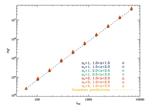
Once the $n_{x}=n_{\ell}n_{z_{bin}}$$(n_{z_{bin}}+1)/2$ dimensional covariance matrix has been computed, we apply Eq. 8 to obtain an estimate ${\bf\hat{C}}^{-1}$. As a first check, we consider a set of Gaussian simulations where the 2D projected density field at each output redshift is replaced by a realisation of a Gaussian field with an identical spectrum as the one resulting from N-body simulations. In that particular case, given the exact number of modes in each $\ell$ shell, we can predict exactly the scaling of the dimensionless cumulative information and compare it with the measurements. We consider different number of source bins and all the associated angular cross-power spectra. The results are displayed in Fig. 2 and an excellent agreement is observed between the analytical predictions (dashed line) and the measured quantities (symbols).

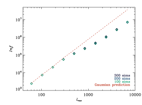
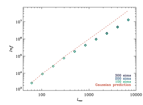
We then move to the genuine N-body simulations and look at the dimensionless information for either one redshift source bin (left panel of Fig. 3) or four redshift source bins (right panel of Fig. 3). In both plots we check the convergence of our result by varying the number of used simulations and compare it with the Gaussian predictions (red dashed line). We considered respectively 100, 200 and 300 simulations. Obviously the convergence is satisfying and much smaller than the effects we are interested in, i.e. the difference between the red dashed line and the symbols. As discussed in Lu et al. (2009), when assessing the convergence of a Monte-Carlo estimator of ${\bf\hat{C}}^{-1}$ is it important to look at ${\bf\hat{C}}^{-1}$ (or its norm) and not the diagonal of ${\bf\hat{C}}$ as in Takahashi et al. (2009). The relative difference between the 200 and 300 simulations computation, probably an upper bound on the convergence, is consistent with our convergence estimate. It is around 8%.

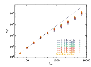
This satisfying convergence is crucial and gives us confidence in the results displayed in Fig. 3. We can now interpret them. First, it is interesting that the saturation effect present in the 3D power spectrum (see Fig. 1) also appears in the convergence power spectrum. As expected, whereas N-body results agree with Gaussian predictions on large (linear) angular scales, a departure from the Gaussian behaviour (red dashed line) appears at sub-degree scales ($\ell>300$). Not surprisingly, for sources between ($1<z<1.5$), this corresponds to $k\simeq 0.2h/$Mpc at $z=0.5$ where the lensing kernel peaks, consistent with what is observed for the 3D power spectrum (at $z=1$) in Fig. 3. When higher redshift sources are included, we are sensitive to higher redshift, we expect the departure from Gaussianity to be milder (non-linear evolution decreases with increasing redshift) and at smaller angular scales (higher $\ell$). This corresponds to what is observed in the right panel of Fig. 3.

This is illustrated furthermore in Fig. 4 where we consider other source redshift distribution. Both the agreement on large scale with the Gaussian prediction and the saturation effect shift to higher $\ell$ with increasing source redshift are clearly visible. So is the decreasing of the saturation effect as the source redshift increases and when tomography is included. As for the 3D case, the information increases in the fully non-linear regime, at a substantially lower value than Gaussian. Note however that the saturation effect is less dramatic than for the 3D case since the projection inherent to lensing introduces an extra Gaussianization.

Figure 4: Dimensionless cumulative information for the convergence cross-power spectra defined in Eq. 5. Each color correspond to a different sub-set of source redshift band of size $n_{z}=$ 1, 2, 3 or 4. The dashed color line corresponds to the Gaussian prediction for the same number of modes. As in 3D, the effect of non-Gaussianity is clearly visible as a drop in the dimensionless information content when one enters the slightly non-linear regime. The scaling becomes Gaussian again in the fully non-linear regime. As expected, since non-linearities increase with redshift, the effect is more severe the lower the source redshift is.

V Discussion

Figure 5: Dark Energy Figure of Merit as a function of scales for 4 various surveys whose parameters are given in Tab. 1. The blue diamonds correspond to the predictions using non-Gaussian covariance matrix and a shot noise contribution. The red diamonds correspond to the Gaussian approximation to the Fisher matrix with shot noise. The orange diamonds correspond to the non-Gaussian case with the prior expected from the Planck satellite. The blue and red dashed curves correspond respectively to the non-Gaussian and Gaussian cases, without shot noise. Whereas we can see that the inclusion of non-Gaussian error bars is important for a perfect noiseless experiment (blue dashed curve) as compared to the perfect noiseless Gaussian errors (red dashed curve), it is less critical when adding the shot noise coming from the dispersion of intrinsic ellipticities (comparison between blue and red diamonds).

Now that we highlighted above the dimensionless cumulative information for some perfect idealized survey of angular area the corresponding to the size of our simulation, we discuss its implications for current and future optical surveys. In particular, we quantify the consequences of the information saturation effects discussed above on the cosmological information content. We focus on DE that we parametrize by an evolving equation of state $w(a)=w_{0}+(1-a)w_{a}$. We use as our main statistic the DE figure of merit (FoM) Albrecht et al. (2006), that we define as the area of the 95% contour ellipse in the $w_{0}-w_{a}$ plane. Following the definition of the Fisher matrix, ${\bf F}$, in Eq. 1, if we consider the following observable

$${\cal P}_{a=z_{i}(z_{i}-1)/2+z_{j},\ell}=\tilde{n}_{z_{i}}\tilde{n}_{z_{j}}C_{\ell}^{\kappa\ z_{i}z_{j}}\,,\quad(i\geq j)$$ (21)

and a set of six cosmological parameters $\alpha_{\mu}$. The Fisher information matrix writes as

$${\bf F}_{\mu\nu}=\sum_{\ell=2}^{\ell_{\rm max}}{\sum_{ab}{\partial{{\cal P}_{a}}\over\partial{\alpha_{\mu}}}[{\bf C}^{-1}]_{ab}{\partial{{\cal P}_{b}}\over\partial{\alpha_{\nu}}}}\,.$$ (22)

With this notation, $\sigma(\alpha_{\mu})=\sqrt{{\bf F}^{-1}_{\mu\mu}}$.

We will still make use of the 300 simulations introduced in Sec. IV and customized for the diffuse 21cm lensing Lu et al. (2009) to discuss optical cosmic shear. We do so by re-weighting the previous results obtained using the wide uniform redshift bins with the relative weights appropriate coming from a realistic optical galaxy density

$$n(z) \propto z^{\alpha}e^{-\left({z/z_{0}}\right)^{\beta}},$$ (23)

$${\rm with\quad}\alpha=2 \quad{\rm and} \beta=1.5.$$ (24)

$\tilde{n}_{i}$ corresponds to the total number of galaxies in the $i$th redshift bin. We also rescale the signal covariance matrix by the survey area considered. Note that in this work, we will ignore the uncertainties in the number density, however important they are Benjamin et al. (2007). We will consider four surveys whose parameters are given in Tab. 1. They roughly correspond respectively to a current survey like CFHTLS , the soon on-line DES survey, and wide and deep space survey like Euclid or JDEM . We will normalize $n(z)$ so that the galaxy density matches the one given on the second line of Tab. 1 and we will consider the shot noise coming from the intrinsic ellipticities of objects. Note that our predictions here are somewhat inaccurate due to the fact we are re-weighting our 21cm simulations and also our ideal survey is somewhat suboptimal since we consider only 4 redshift bins to perform tomography, which has been shown to be slightly sub-optimal Ma et al. (2005). However, our treatment is accurate enough to discuss the effects of non-Gaussianities that are the focus of our study.

As a reference point, we will also compute the Fisher matrix with a Gaussian approximation to ${\bf C}^{-1}$. Doing so, we follow the formalism laid out for example in Ma et al. (2005). In the Gaussian case, assuming a shot noise level and simple Gaussian sample variance, the covariance matrix is defined as

$${\bf C}_{ab\ \ell}=\tilde{n}_{i}\tilde{n}_{j}\tilde{n}_{k}\tilde{n}_{l}\left(C^{\rm tot\ ik}_{\ell}C^{\rm tot\ jl}_{\ell}+C^{\rm tot\ il}_{\ell}C^{\rm tot\ jk}_{\ell}\right)\,,$$ (25)

where $a=i(i-1)/2+j$, $b=k(k-1)/2+l$ and where the total power spectrum is

$$C^{\rm tot\ ij}_{\ell}=C_{\ell}^{\kappa\ ij}+\delta_{ij}{\gamma_{\rm int}^{2}\over{\tilde{n}}_{i}}\,,$$ (26)

where $\gamma_{\rm int}$ is the rms shear error per galaxy per component contributed by intrinsic ellipticity and measurement error.

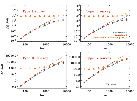
Fig. 5 compares the Gaussian and non-Gaussian cases for the 4 different surveys whose parameters are defined in Tab. 1. Going from the Type I survey to the Type IV survey, we increase simultaneously the number of galaxies, the depth, the number of source redshift bins and the survey area hence an increase in FoM. As we previously did for the dimensionless information content, we will now study the evolution of the FoM as we increase the number of modes, and go from the linear regime to the non-linear regime. This is a proxy to quantify the cosmological interpretation in this survey as we increase angular sensitivity. The red dashed lines corresponds to the noise free Gaussian approximation while the blue dash line corresponds to the non-Gaussian noise free evaluation. As we can see when comparing these two curves, the saturation effect discovered earlier in the cumulative information translates naturally in the evolution of the FoM with $\ell_{max}$. In the case of a noiseless survey, the difference in FoM at high angular resolution can be as high as a factor of  4, even when we consider four tomographic bins. This effect is thus important and in stark contrast with the scaling with $\ell_{max}$ usually assumed in the literature (e.g. Amara and Refregier (2007)). However, when introducing realistic levels of noise, the effect is somewhat mitigated as is visible when comparing the red diamonds (gaussian approximation, with noise) to the blue diamond (non-gaussian covariance matrix, with noise). It is still however non-negligible since the ratio between the Gaussian and non-Gaussian cases at higher $\ell_{max}$ becomes closer to 1.6. This point constitutes the key result from our study. While potentially very damaging to the ideal performances of weak gravitational surveys, the effect of non-Gaussianity is tampered by the estimated level of Gaussian noise expected for current and future surveys. The inclusion of the Planck prior does not affect those conclusions at high $\ell$.

Note also that despite the fact that our plot hint at the ability to measure the convergence power spectra up to $\ell<10000$, in practice, it will most likely be limited by theoretical uncertainties at $\ell\leq 3000$, not the least by our inability to model the details of the baryon physics White (2004); Zhan and Knox (2004); Rudd et al. (2007).

Figure 6: Bootstrap errors on the ratio between the noiseless FoM curves for the Type IV survey. We are thus plotting the ratio between the red and blue dashed curve in the lower right panel of Fig. 5

Figure 7: Dimensionless cumulative information content as a function of maximum multipole for a source plane at $z=1000$. A mild saturation effect is still visible. Since the CMB lensing is sensitive mostly to the growth of structure at $z\simeq 2.5$, the saturation effect is milder and shifted to smaller angular scales (higher $\ell_{max}$).

Table 1: Optical surveys considered

Survey	I	II	III	IV
$Area$ (deg.2)	200	200	5 000	20 000
$n_{gal}$ (#/arcmin.2)	30	30	50	100
$\langle\gamma\rangle$	0.25	0.25	0.25	0.25
# redshift bins	1	3	3	4

Consistent conclusions were reached in the halo model based analytical approach followed in Cooray and Hu (2001); Takada and Jain (2008). We will discuss the latter as being the most recent and refer to its discussion of the earlier results of Cooray and Hu (2001). Our results seem consistent with their evaluation of the signal to noise ratio (somewhat comparable to our dimensionless information). So does the effects on parameters when considering realistic surveys although our factor of  1.6 for FoM seems a bit higher. Note however that the comparison is not direct since the set of parameters we consider is slightly different. Whereas we consider a flat Universe with 6 parameters including an evolving DE equation of state, they consider non-flat models and allow the spectral index to run. We did not translate our evaluation of the cross-power spectrum covariance matrices to real space statistics and therefore we refer the reader to the discussion of Takada and Jain (2008) for a comparison with real space evaluation of this effect, as e.g. Semboloni et al. (2007). A more detailed comparison between analytical estimates and numerical work would be instructive and has to be performed but we leave it for further work. So do we for the dependence of our results on cosmological parameters, mostly $\sigma_{8}$, $n_{s}$ and $\Omega_{m}$ Eifler et al. (2008). Note that we also do not investigate the so-called “beat-coupling” effect Hamilton et al. (2006); Takada and Jain (2008). As we understand it, it denotes the extra-mode coupling induced by the finiteness of the observed volume, i.e. such an effect would be non-existent if the all-sky was considered. Since the exact form of this coupling will depend on the exact mask of any given survey, we decided to ignore this effect here. In practice, as it is usually performed for example while analysing CMB data, we would start from a mask description in real space and propagate the induced mode-coupling in Fourier space throughout all our calculations Padmanabhan et al. (2003) with special care to the peculiarities of non-Gaussian statistics. With their own prescription, Takada and Jain (2008) found that it does not affect qualitatively the effect of the non-linear growth of structures.

The comparison with the numerical work of Hu and White (2001) is also not obvious. First, a different cosmology with a higher $\sigma_{8}$ is considered, which should enhance the non-linear effect. Second, they consider 200 simulations and a standard tilling technique that should give rise to an accuracy of at most at most 85% on the errors using the scaling formula of Takahashi et al. (2009). All those reasons make a direct comparison a bit difficult.

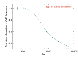
To quantify further the error on the errors issue, we evaluate the errors of the FoM for the Type IV survey introduced before using a bootstrap method discussed above. We display the results in Fig. 6 where we plotted the relative difference between the Gaussian and non-Gaussian FoM as a function of $\ell_{max}$. Due to the strong convergence properties of our covariance estimation technique, we quantify the error on the errors to be around 25% on large scale and sub-percent on the smaller scales we consider. This fact certainly constitutes an improvement over previous results in the literature and is consistent with our estimate of a 1/$\sqrt{n_{sim}n_{box}}$ convergence rate. If we use the scaling of 12/$\sqrt{n_{sim}}$ measured by Takahashi et al. (2009), we claim an overal uncertainty due to the limited number of simulations to be around 14%.

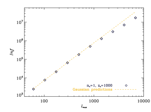
Besides the optical observations of weak-gravitational lensing, the cosmic microwave background (CMB) constitutes another source plane where lensing can be observed (see Lewis and Challinor (2006) for a review). As both the resolution and the sensitivity of detectors improve, it can now be measured and it defines the next frontier for the CMB temperature and polarization measurement Smith et al. (2008). Using cross correlation between WMAP data and other tracers of large scale structures to increase the signal to noise, a detection of gravitational lensing in the CMB temperature has been achieved with marginal significance, i.e. around 2.4 $\sigma$ Hirata et al. (2004); Smith et al. (2007); Hirata et al. (2008). A direct detection in temperature is expected to be achieved soon with high significance thanks to on-going high angular resolution temperature surveys (ACT, SPT, Planck). It is thus interesting to evaluate the effects of the non-linear growth of structures on the CMB lensing signal. To do so, we compute the cumulative information as a function of maximum angular scale $\ell_{max}$, when considering one redshift source plane at $z=1000$. The result is displayed in Fig. 7. Interestingly, the saturation effect is still visible, and not surprisingly, since the CMB lensing kernel peaks around z$\simeq 2.5$, the effect is smaller and shifted to smaller scales. In practice however, given that the CMB reconstruction is most likely going to be limited by secondary anisotropies (kinetic SZ in particular and patchy reionization) around a few $\ell\simeq 3000$, it is unlikely that this effect of non-linear growth will be a critical effect.

To conclude, non-Gaussian effects are potentially very important for weak-gravitational surveys and might alter significantly the forecasts done so far. When considering realistic noise estimate for the coming optical surveys, the impact of non-Gaussian error bars is much milder. However, an interesting indirect consequences of our study is the sub-Gaussian scaling of information in the fully non-linear regime (this was also observed in the 3D power spectrum Rimes and Hamilton (2006)). This fact highlights the great information gain that can be make by studying this regime, both using 2 point statistics but also higher order more specific to non-Gaussian effects. Nevertheless, it will require more theoretical insights.