Theoretical Analysis of Cyclic Frequency Domain Noise and Feature Detection for Cognitive Radio Systems

Abstract

In cognitive radio systems, cyclostationary feature detection plays an important role in spectrum sensing, especially in low SNR cases. To configure the detection threshold under a certain noise level and a pre-set miss detection probability $P_{f}$, it’s important to derive the theoretical distribution of the observation variable. In this paper, noise distribution in cyclic frequency domain has been studied and Generalized Extreme Value (GEV) distribution is found to be a precise match. Maximum likelihood estimation is applied to estimate the parameters of GEV. Monte Carlo simulation has been carried out to show that the simulated ROC curve is coincided with the theoretical ROC curve, which proves the efficiency of the theoretical distribution model.

I Introduction

Spectrum sensing plays an important role in cognitive radio (CR) systems, and cyclostationary feature detection is one of the main technologies for spectrum sensing in low SNR cases [1-2]. The idea of cyclic detection is that one CR node samples the RF signals, transform the time domain signals into cyclic frequency domain, then decide primary user’s occupancy of a target band regarding whether the cyclic spectrum on a significant cyclic frequency is above a certain threshold [2].
Although the simulation results of cyclostationary feature detection has been studied [3-5], less attention has been paid to analyze the noise distribution on cyclic frequency domain. Consequently, theoretical function between detection threshold $\lambda_{th}$ and miss detection probability $P_{f}$ is not available, which makes it difficult for practical system design. For comparison, the theoretical function between detection threshold $\lambda_{th}$ and miss detection probability $P_{f}$ of energy detection is available by using central and non-central chi-square distribution to model the distribution of the observation variable affected by time domain Gaussian noise [6], which makes energy detection to be a practical method for spectrum sensing. However, its performance in low SNR cases is much poorer than cyclostationary feature detection [7]. In this paper, noise distribution on cyclic frequency domain has been analyzed and generalized extreme value distribution is found to be a precise match of the observation variable affected by time domain Gaussian noise. A fast cyclic frequency domain feature detection algorithm [7] has been introduced to evaluate the coincidence between theoretical ROC curve and the simulated ROC curve, which proves the reliability of theoretical distribution model and feasibility of practical system design.
The rest part of the paper is organized as follows: Section II describes the system model of cyclostationary feature detection. Noise distribution on cyclic frequency domain is analyzed in section III. A fast cyclic frequency domain feature detection algorithm has been introduced in section IV. Simulation results are given in Section V. Finally, conclusions are drawn in Section VI.

II SYSTEM MODEL

The spectrum sensing problem can be modeled as hypothesis testing. It is equivalent to distinguishing between the following two hypotheses:

$$\left\{\begin{array}[]{l}H_{0}:y(t)=n(t)\\ H_{1}:y(t)=x(t)+n(t)\\ \end{array}\right.$$ (1)

$y(t)$, $x(t)$ and $n(t)$ denote the received signal, the primary user’s transmit signal and the Gaussian noise, respectively. $H_{1}$ and $H_{0}$ represent the hypothesis that the primary user is active or inactive. Due to the existence of noise, a certain threshold $\lambda_{th}$ should be set to decide whether a primary user is active or not. Probability of detection ($P_{d}$) and false alarm ($P_{f}$) are defined to evaluate the detection performance:

$$\left\{\begin{array}[]{l}P_{d}=p(y_{i}>\lambda_{th}|H_{1})\\ P_{f}=p(y_{i}>\lambda{th}|H_{0})\\ \end{array}\right.$$ (2)

The goal of detection is to maximize $P_{d}$ while maintain a given $P_{f}$.
When feature detection is applied, the detection model (1) changes into:

$$\left\{\begin{array}[]{l}H_{0}:S_{y}^{\alpha}(f)=S_{n}^{\alpha}(f)\\ H_{1}:S_{y}^{\alpha}(f)=S_{x}^{\alpha}(f)+S_{n}^{\alpha}(f)\\ \end{array}\right.$$ (3)

$S_{y}^{\alpha}(f)$ is the spectrum correlation density (SCD) of the received signal $y(t)$, $S_{x}^{\alpha}(f)$ and $S_{n}^{\alpha}(f)$ is the SCD of $x(t)$ and $n(t)$, respectively [8].

Theoretically, Gaussian noise $n(t)$ is not a cyclostationary statistic process, then $S_{n}^{\alpha}(f)=0$ when $\alpha\neq 0$ [8]. As for cyclostationary signal $x(t)$, there is a significant frequency set {$\alpha_{0}$}, on which $S_{x}^{\alpha_{0}}(f)\neq 0$. Due to the ideal non-cyclostationary characteristic of Gaussian noise, any pre-set threshold $\lambda_{th}$ on a significant frequency will lead to $P_{d}=1$ and $P_{f}=0$.

III Noise distribution on cyclic frequency domain

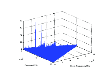
In practice, SCD is calculated for limited length signals, therefore, $S_{n}^{\alpha}(f)\neq 0$ when $\alpha\neq 0$ [9]. As shown in Fig.1, the background noise is obvious on $f\sim\alpha$ square when calculating SCD of a noise interfered AM modulated signal.

Figure 1: Cyclic Spectrum Density of AM at SNR=-10db

In order to analyze the background noise distribution, a limited-length Gaussian noise sequence $n^{iK}(j)$ is considered:

$$n^{iK}(j)=\left\{\begin{array}[]{l}n(iK+j),0\leq j\leq K-1\\ 0,else\\ \end{array}\right.$$ (4)

where $K$ is the length of the analysis window, $i=0,1,...,\infty$ is the index of analysis window. Noise data in each analysis window are transformed into cyclic frequency domain, and then mapped from $f\sim\alpha$ square to $\alpha$ axis through the following expression:

$$N^{iK}(\alpha)=\max_{f}|S_{n}^{\alpha}(f)|$$ (5)

For each cycle frequency $\alpha_{0}$, the cyclic spectrum value is aligned to a set {$N_{i}=N^{iK}(\alpha_{0})$}, $i=0,1,...,L$. According to the extreme definition of $N^{iK}(\alpha_{0})$ in (5), Generalized Extreme Value (GEV) distribution is adopted to model the cyclic frequency domain noise [10]. The density function is:
when $\kappa\neq 0$

$$f(x|\kappa,\mu,\sigma)=(\frac{1}{\sigma})e^{(-(1+\kappa\frac{(x-\mu)}{\sigma})^{-\frac{1}{\kappa}})}(1+\kappa\frac{(x-\mu)}{\sigma})^{-1-\frac{1}{\kappa}}$$ (6)

when $\kappa=0$

$$f(x|0,\mu,\sigma)=(\frac{1}{\sigma})exp(-exp(-\frac{x-\mu}{\sigma})-(-\frac{x-\mu}{\sigma}))$$ (7)

where $\kappa$ is the shape parameter, $\mu$ is the position parameter, $\sigma>0$ is the scale parameter. And the parameters $\kappa$ , $\mu$ , $\sigma$ can be estimated by maximum likelihood estimation based on the noise sequence {$N_{i}$}. For most cases, $\kappa\approx 0$, then the likelihood function is defined as follows:

$$l(\mu,\sigma)=-Lln\sigma-\sum_{i=1}^{L}(\frac{N_{i}-\mu}{\sigma})-\sum_{i=1}^{L}exp\{-(\frac{N_{i}-\mu}{\sigma})\}$$ (8)

Let $\frac{\partial l}{\partial\mu}=0$,$\frac{\partial l}{\partial\sigma}=0$ then:

$$\left\{\begin{array}[]{l}\sum_{i=1}^{L}e^{-(N_{i}-\hat{\mu})}/\hat{\sigma}=L\\ \sum_{i=1}^{L}(N_{i}-\hat{\mu})(1-e^{-(N_{i}-\hat{\mu})/\hat{\sigma}})=L\hat{\sigma}\\ \end{array}\right.$$ (9)

where $\hat{\mu}$ and $\hat{\sigma}$ are the estimated value of $\mu$ and $\sigma$. By solving (9), $\hat{\mu}$ and $\hat{\sigma}$ are obtained.
After that, the likelihood function for $\kappa$ is defined as:

$$l(\kappa,\hat{\mu},\hat{\sigma}) = -Nln\hat{\sigma}-(1+\frac{1}{\kappa})\sum_{i=1}^{N}ln[1+\kappa(\frac{n_{i}-\hat{\mu}}{\hat{\sigma}})]$$ (10)

$$-\sum_{i=1}^{N}[1+\kappa(\frac{n_{i}-\hat{u}}{\hat{\sigma}})]^{-\frac{1}{\kappa}}$$

Let $\frac{\partial l}{\partial\kappa}=0$, the estimation of $\hat{\kappa}$ can be obtained by solving (10).

IV Fast Cyclic Frequency Domain Feature Detection Algorithm

Fig.2 shows the block diagram of a cyclic frequency domain feature detector [7]:

Figure 2: Block diagram of a feature detector

In this detector, time domain signals are transformed to cyclic frequency domain, and then mapped to $\alpha$ axis and get extreme value for each $\alpha$, finally, compared with a pre-set threshold $\lambda_{th}$ to determine the occupancy of primary user. To decrease the computational complexity of feature detection, only one cycle frequency $\alpha_{0}$ for a modulated signal is calculated for spectrum sensing [7]. The probability of detection ($P_{d}$) and false alarm ($P_{f}$) is defined by:

$$\left\{\begin{array}[]{l}P_{d}=Pr(T>\lambda_{th}|H_{1})\\ P_{f}=Pr(T>\lambda{th}|H_{0})\\ \end{array}\right.$$ (11)

where $Pr(\cdot)$ is CDF of generalized extreme value distribution. Substitution of (6) and (7) into (11) yields:

$$P_{f}=Pr(T>\lambda_{th}|H_{0})=\int_{\lambda_{th}}^{+\infty}f(x|\hat{\kappa},\hat{\mu},\hat{\sigma})dx$$ (12)

For a pre-set $P_{f}$, the threshold can be estimated as:

$$\lambda_{th}=\left\{\begin{array}[]{l}\hat{\mu}-\frac{\hat{\sigma}}{\hat{\kappa}}(1-y_{p}-\hat{\kappa}),\hat{\kappa}\neq 0\\ \hat{\mu}-\hat{\sigma}logy_{p},\hat{\kappa}=0\\ \end{array}\right.$$ (13)

where $y_{p}=-log(1-P_{f})$.

V Simulation Results

In this section, Monte-Carlo simulation results are presented to prove the reliability of the upper analytical results between $P_{f}$ and the threshold $\lambda_{th}$.
Frequency smoothing method in [11-12] is applied to estimate SCD of a time domain noise signal. Simulation parameters are listed in TABLE 1. Length of the analysis window is set to be 4096 and totally 10000 cyclic spectrum values on cyclic frequency $\alpha_{0}=2f_{c}$, aligned by analysis window index, are considered to evaluate the theoretical curve.

TABLE I: Simulation parameters list

Parameter	Value
Modulation type	AM
Carrier frequency	1 MHz
Bandwidth	10 KHz
Sampling frequency	3 MHz
Sampling time	1.365ms
Channel	AWGN
Window type	hamming
Frequency smoothing length	1300
Sampled data length(K)	4096

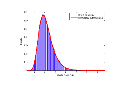
The histogram of the aligned cyclic spectrum values is shown in Fig 3, with compared to GEV distribution. It is proved that the GEV distribution precisely match the cyclic frequency domain noise data.

Figure 3: GEV curve for the noise samples

For further proof of the proposed model, the curves of receiver operating characteristics (ROC) , which are theoretically derived from GEV distribution, are plotted to compare with those derived from Monte-Carlo simulation. As to the theoretical curve, $P_{f}$ is pre-set according to system requirement. By using (13), a theoretical threshold $\lambda_{th}$ is obtained. Finally, received signals under hypothesis $H_{1}$ are compared with the threshold to obtain the statistics result of $P_{d}$. As to the simulated curve, threshold are chosen to be the same as the theoretical threshold {$\lambda_{th}$}, after that, received signals under hypothesis $H_{1}$ and $H_{0}$ are compared with each $\lambda_{th}$ to obtain the statistics results of $P_{d}$ and $P_{f}$. Finally, plot these ($P_{d}$,$P_{f}$) points to form a continuous curve.
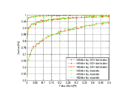
Experiments results are shown in Fig.4, we can see that the theoretical ROC curve (red highlighted) precisely match the simulated ROC curve (green highlighted) for different received signal power levels. It is proved that the generalized extreme value distribution is efficient to model the noise distribution on cyclic frequency domain.

Figure 4: ROC curves under different signal power levels

VI Conclusion

In this paper, noise distribution on cyclic frequency domain is studied and generalized extreme value (GEV) distribution is found to be an efficient method to model the cyclic frequency domain noise. Maximum likelihood estimation is applied to estimate the parameters of GEV. Sensing threshold is consequently derived from system requirements (a pre-set $P_{f}$) and theoretical CDF of GEV distribution. Monte Carlo simulation has been carried out to prove that the simulated ROC curve is precisely coincided with the theoretical ROC curve.

References

- [1] William A. Gardner, and Chad M. Spooner, ”Detection and Source Location of Weak Cyclostationary Signals: Simplifications of the Maximum-Likelihood Receiver”, IEEE Trans. Commun., vol-41, NO. 6, JUNE 1993.
- [2] Paul D. Sutton, Keith E. Nolan, and Linda E. Doyle, ”Cyclostationary Signatures in Practical Cognitive Radio Applications”, Selected Areas in Commun, IEEE Journal vol.26, Issue 1, pp. 13 - 24, Jan. 2008.
- [3] Punchihewa, A. Dobre, O.A. Rajan, S. Inkol, R.; ”Cyclostationarity-based Algorithm for Blind Recognition of OFDM and Single Carrier Linear Digital Modulations”, PIMRC 2007.
- [4] Zhuan Ye, John Grosspietsch, and Gokhan Memik, ”Spectrum Sensing Using Cyclostationary Spectrum Density for Cognitive Radios”, Signal Processing Systems, 2007 IEEE Workshop, pp. 1-6, Oct. 2007.
- [5] Sutton, P.D. Nolan, K.E. Doyle, L.E. ”Cyclostationary Signatures for Rendezvous in OFDM-Based Dynamic Spectrum Access Networks”,DySPAN 2007
- [6] Jun Ma, Guodong Zhao, and Ye Li, ”Soft Combination and Detection for Cooperative Spectrum Sensing in Cognitive Radio Networks,” IEEE Transactions on Wireless Communications, vol. 7, no. 11, pp. 4502 - 4507, November 2008.
- [7] Shan Da, Gan Xiaoying, Chen Hsiao-Hwa, Qian Liang, Fast Cycle Frequency Domain Feature Detection for Cognitive Radio Systems, IEEE Crowncom 2009, submitted. (arXiv.org, arXiv:0903.1183v1)
- [8] W. Gardner, ”The spectral correlation theory of cyclostationary time-series”, Signal Processing, Vol.11(1), pp.13-36, 1986.
- [9] Gan Xiaoying, Xu Hao, Xu Youyun, Qian Liang, Liu Jing, ”Noise analysis for limited length cyclostationary detection in cognitive radio systems”, Journal of PLA University of Science and Technology,2008, vol. 9, No.6, pp:633-636.
- [10] Balakrishnan N., Nevzorov V.B., A Primer on Statistical Distributions, Wiley InterScience, pp. 193-194, 2003.
- [11] W.A. Gardner, ”Measurement of Spectral Correlation”, IEEE Trans. on Acoustics, Speech, and Signal Processing, VOL. ASSP-34, NO. 5, Oct. 1986.
- [12] W.A. Gardner, ”Digital Implementations of Spectral Correlation Analyzers”, IEEE Trans. on Signal Processing, VOL 41, NO 2, Feb. 1993.