Search for gravitational-wave bursts in the first year of the fifth LIGO science run
Abstract
We present the results obtained from an all-sky search for gravitational-wave (GW) bursts in the 64–2000 Hz frequency range in data collected by the LIGO detectors during the first year (November 2005 – November 2006) of their fifth science run.The total analyzed livetime was 268.6 days. Multiple hierarchical data analysis methods were invoked in this search. The overall sensitivity expressed in terms of the root-sum-square (rss) strain amplitude for gravitational-wave bursts with various morphologies was in the range of Hz-1/2 to a few Hz-1/2. No GW signals were observed and a frequentist upper limit of 3.75 events per year on the rate of strong GW bursts was placed at the 90% confidence level. As in our previous searches, we also combined this rate limit with the detection efficiency for selected waveform morphologies to obtain event rate versus strength exclusion curves. In sensitivity, these exclusion curves are the most stringent to date.
pacs:
04.80.Nn, 07.05.Kf, 95.30.Sf, 95.85.SzThe LIGO Scientific Collaboration, http://www.ligo.org ]Dated:
I Introduction
After many years of preparation, interferometric gravitational wave (GW) detectors have now begun an era of long-duration observing. The three detectors of the Laser Interferometer Gravitational-Wave Observatory (LIGO) Abbott et al. (2009a) reached their design sensitivity levels in 2005 and began a “science run” that collected data through late 2007. This run is called “S5” since it followed a sequence of four shorter science runs that began in 2002. The German/British GEO600 detector H. Grote (2008) (for the LIGO Scientific Collaboration) joined the S5 run in January 2006, and the Italian/French Virgo detector Acernese et al. (2006) began its first science run (denoted VSR1) in May 2007, overlapping the last months of the S5 run. The data collected by these detectors provide the best opportunity yet to identify a GW signal—though detection is still far from certain—and is a baseline for future coordinated data collection with upgraded detectors.
Gravitational waves in the frequency band of LIGO and the other ground-based detectors may be produced by a variety of astrophysical processes Culter and Thorne (2002). See for example Blanchet (2006) for inspiralling compact binaries, Jaranowski and Schutz (1998) for spinning neutron stars, J. Baker, J.Centrella, D. Choi, M. Koppitz, and J. van Meter (2006) for binary mergers, and Ott et al. (2004, 2006); C. D. Ott, H. Dimmelmeier, A. Marek, H-T Janka, B. Zink, I. Hawke and E. Schnetter (2007); Ott (2009) for core-collapse supernovae.
The GW waveform emitted by a compact binary system during the inspiral phase can be calculated accurately in many cases, allowing searches with optimal matched filtering; see, for example, Abbott et al. (2008a). The waveform from the subsequent merger of two black holes is being modeled with ever-increasing success using numerical relativity calculations, but is highly dependent on physical parameters and the properties of strong-field gravity. The uncertainties for the waveforms of other transient sources are even larger. It is thus desirable to explore more generic search algorithms capable of detecting a wide range of short-duration GW signals from poorly-modeled sources—such as stellar core collapse to a neutron star or black hole—or unanticipated sources. As GW detectors extend the sensitivity frontier, it is important to not rely too heavily on assumptions about source astrophysics or about the true nature of strong-field gravity, and to search as broadly as possible.
In this paper, we report on a search for GW “burst” signals in the LIGO data that were collected during the first 12 months of the S5 science run. A search for GW bursts in the remainder of the S5 data set, along with the Virgo VSR1 data, will be published jointly by the LSC and Virgo collaborations at a later date.
The GW burst signals targeted are assumed to have signal power within LIGO’s frequency band and durations shorter than 1 s, but are otherwise arbitrary. This analysis, like most of our previously published searches for GW bursts, focuses on low frequencies—in this case 64 Hz to 2000 Hz—where the detectors are the most sensitive. A dedicated search for bursts above 2000 Hz is presented in a companion paper Abbott et al. (2009b).
Interferometric GW detectors collect stable, high-sensitivity (“science mode”) data typically for several hours at a time, with interruptions due to adverse environmental conditions, maintenance, diagnostics, and the need to occasionally regain the “locked” state of the servo controls. In this analysis we searched the data at all times when two or more LIGO detectors were operating, a departure from the all-sky GW burst searches from earlier science runs Abbott et al. (2005a, b, 2006, 2007, 2008b), which required coincidence among three (or more) detectors. In this paper, the term “network” is used to describe a set of detectors operating in science mode at a given time. A network may include any combination of the Hanford 4 km (H1) and 2 km (H2) detectors, the Livingston 4 km (L1) detector and GEO600. Because the GEO600 detector was significantly less sensitive than LIGO during the S5 run (a factor of 3 at 1000 Hz, and almost two orders of magnitude at 100 Hz), we do not use its data in the initial search but reserve it for evaluating any event candidates found in the LIGO data.
This paper presents results from three different “analysis pipelines”, each representing a complete search. While the pipelines analyzed the data independently, they began with a common selection of good-quality data and applied a common set of vetoes to reject identifiable artifacts. Each pipeline was tuned to maximize the sensitivity to simulated GW signals while maintaining a fixed, low false alarm rate. The tuning of the pipelines, the choice of good data and the decision on the veto procedure were made before looking at potential candidates.
No GW signal candidates were identified by any of the analysis pipelines with the chosen thresholds. In order to interpret this non-detection, we evaluate the sensitivity of each pipeline for simulated signals of various morphologies, randomly distributed over the sky and over time. As expected, there are some sensitivity differences among the pipelines, although the sensitivities rarely differ by more than a factor of 2 (see section VII) and no single pipeline performs best for all of the simulated signals considered. We combine the results of the pipelines to calculate upper limits on the rate of GW bursts as a function of signal morphology and strength.
The rest of the paper is organized as follows: After specifying the periods of data, forming the first year of the S5 science run in Sec. II, Sec. III describes the state of the detectors during that period. Section IV summarizes the elements of this GW burst search which are common to all of the analysis pipelines. The analysis pipelines themselves are detailed in Sec. V and Appendices C, D and E. Section VI describes how each pipeline is tuned, while Sec. VII presents the sensitivity curves for simulated signals and Sec. VIII describes the systematic errors in these sensitivity curves. The results of the search are given in Sec. IX, and some discussion including estimates of the astrophysical reach for burst candidates in Sec. X.
II S5 First-Year Data Set
The search described in this paper uses data from approximately the first calendar year of S5, specifically from November 4, 2005 at 16:00 UTC through November 14, 2006 at 18:00 UTC.
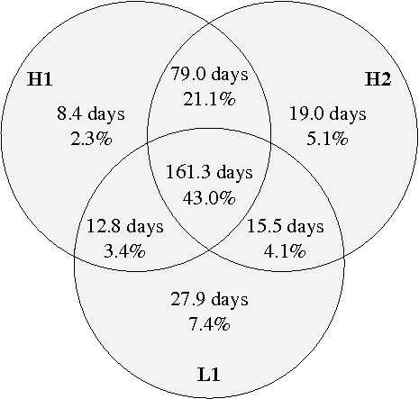
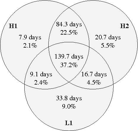
Figure 1 shows the amount of science-mode data collected (“livetime”) for each mutually-exclusive network of detectors along with percentages of the experiment calendar duration (duty cycle). The top Venn diagram represents the data with basic data quality and veto conditions (see Sec. IV and Appendices A and B), including days of data during which two or more LIGO detectors were in science mode; this is the sample which is searched for GW burst signals. An explicit list of the analyzed intervals after category 2 DQFs is available at Hughey (2009). The bottom Venn diagram shows the livetimes after the application of additional data quality cuts and vetoes that provide somewhat cleaner data for establishing upper limits on GW burst event rates. In practice, only the H1H2L1 and H1H2 (not L1) networks—encompassing most of the livetime, 224 days—are used to set upper limits.
III The detectors
III.1 LIGO
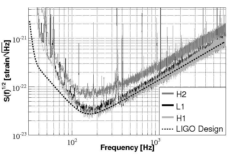
The high sensitivity (see Fig. 2) and duty cycles (78.0% for H1, 78.5% for H2, and 66.9% for L1) achieved during the S5 run were the result of a number of improvements made prior to the run Sigg et al. (2006); Waldman et al. (2006). The major changes were the successful operation at Livingston of a hydraulic external pre-isolator (HEPI) to suppress seismic disturbances, and the implementation at both sites of a thermal compensation system (TCS) to reduce thermal lensing effects in the interferometer arm cavities due to optical absorption in mirror coatings and substrates. The HEPI system provides a reduction of the seismic noise by an order of magnitude in the band 0.2–2.0 Hz, and thus significantly improves the duty cycle of the L1 detector.
Another significant improvement was the extension of the wave-front sensing (WFS) subsystem to control all alignment degrees of freedom of the core interferometer optics, leading to significantly reduced alignment fluctations. Several improvements were made to the length sensing and control subsystem, enabling the photodetectors to take more power without saturation and thus allowing the laser power to be increased. A new method to calibrate the detectors was introduced, based on direct actuation of the test masses via radiation pressure from an auxiliary laser beam. Unlike the traditional coil-drive calibration method R. Adhikari, G. Gonzalez, M. Landry and B. O’Reilly (2003), which requires rather large test mass displacements, the new technique allows calibration of the detectors at a level closer to the anticipated signal strength.
Other improvements included modifications to acoustic and seismic isolation of optical tables with detection photodiodes, changes to the safety shutters to protect photodiodes from damage when interferometers fall out of lock, and improved detection of impending saturation of photodiodes to prevent lock losses. Finally, a number of physical effects which led to spurious transients and spectral lines in the data during previous science runs have been diagnosed and mitigated.
III.2 GEO600
The GEO600 detector, located near Hannover, Germany, was also operational during the S5 run, though with a lower sensitivity than the LIGO detectors. The GEO600 data were not used in the current study as the modest gains in the sensitivity to GW signals would not have offset the increased complexity of the analysis. The GEO600 data were held in reserve, and could have been used to follow up on detection candidates from the LIGO-only analysis.
GEO600 began its participation in S5 on January 21, 2006, operating in a night-and-weekend mode. In this mode, science data were acquired during nights and weekends while commissioning work was performed during the day time. The commissioning work focused mainly on gaining a better understanding of the detector and improving data quality. It was performed in a manner that avoided disrupting science periods and allowed for well-calibrated data to be acquired. Between May 1 and October 6, 2006, GEO600 operated in so-called 24/7-mode, during which the detector’s duty cycle in science-mode operation was maximized and only very short maintenance periods took place. Overall in 24/7-mode an instrumental duty cycle of about 95% and a science-mode duty cycle of more than 90% were achieved. GEO600 returned to night-and-weekend mode on October 16, 2006, and work began on further improving the reliability of the instrumentation and reducing the glitch rate. The detector was operated in night-and-weekend mode until the end of S5 in October 2007. Overall, GEO600 collected about 415 days of well-calibrated and characterized science data in the period between January 2006 and October 2007.
IV Analysis pipeline overview
In this search for GW bursts, three independent end-to-end analysis pipelines have been used to analyze the data. These pipelines were developed and implemented separately, building upon many of the techniques that were used in previous searches for bursts in the S1, S2, S3 and S4 runs of LIGO and GEO600 Abbott et al. (2004, 2005a, 2006, 2007, 2008b), and prove to have comparable sensitivities (within a factor of ; see Sec. VII). One of these pipelines is fully coherent in the sense of combining data (amplitude and phase) from all detectors and accounting appropriately for time delays and antenna responses for a hypothetical gravitational-wave burst impinging upon the network. This provides a powerful test to distinguish GW signals from noise fluctuations.
Here we give an overview of the basic building blocks common to all of the pipelines. The detailed operation of each pipeline will be described later.
IV.1 Data quality evaluation
Gravitational-wave burst searches are occasionally affected by instrumental or data acquisition problems as well as periods of degraded sensitivity or nonstationary noise due to bad weather or other environmental conditions. These may produce transient signals in the data and/or may complicate the evaluation of the significance of other candidate events. Conditions which may adversely affect the quality of the data are catalogued during and after the run by defining “data quality flags” (DQFs) for lists of time intervals. DQFs are categorized according to their seriousness; some are used immediately to select the data to be processed by the analysis pipelines (a subset of the nominal science-mode data), while others are applied during post-processing. These categories are described in more detail in Appendix A. In all cases the DQFs were defined and categorized before analyzing unshifted data to identify event candidates.
IV.2 Search algorithms
Data that satisfies the initial selection criteria are passed to algorithms that perform the signal-processing part of the search, described in the following section and in three appendices. These algorithms decompose the data stream into a time-frequency representation and look for statistically significant transients, or “triggers”. Triggers are accepted over a frequency band that spans from 64 Hz to 2000 Hz. The lower frequency cut-off is imposed by seismic noise which sharply reduces sensitivity at low frequencies, while the upper cut-off corresponds roughly to the frequency at which the sensitivity degrades to the level found at the low frequency cut-off. (A dedicated search for bursts with frequency content above 2000 Hz is presented in a companion paper Abbott et al. (2009b).)
IV.3 Event-by-event DQFs and vetoes
After gravitational-wave triggers have been identified by an analysis pipeline, they are checked against additional DQFs and “veto” conditions to see if they occurred within a time interval which should be excluded from the search. The DQFs applied at this stage consist of many short intervals which would have fragmented the data set if applied in the initial data selection stage. Event-by-event veto conditions are based on a statistical correlation between the rate of transients in the GW channel and noise transients, or “glitches”, in environmental and interferometric auxiliary channels. The performance of vetoes (as well as DQFs) are evaluated by the extent to which they remove the GW channel transients of each interferometer, as identified by the KleineWelle (KW) Blackburn et al. (2005) algorithm. KW looks for excess signal energy by decomposing a timeseries into the Haar wavelet domain. For each transient, KW calculates a significance defined as the negative of the natural logarithm of the probability, in Gaussian noise, of observing an event as energetic or more than the one in consideration. The veto conditions, like the DQFs, were completely defined before unshifted data was analyzed to identify gravitational-wave event candidates. A detailed description of the implementation of the vetoes is given in Appendix B.
IV.4 Background estimation
In order to estimate the false trigger rate from detector noise fluctuations and artifacts, data from the various detectors are artificially shifted in time so as to remove any coincident signals. These time-shifts have strides much longer than the intersite time-of-flight for a true gravitational-wave signal and thus are unlikely to preserve any reconstructable astrophysical signal when analyzed. We refer to these as time-shifted data. Both unshifted and time-shifted data are analyzed by identical procedures, yielding the candidate sample and the estimated background of the search, respectively. In order to avoid any biases, no unshifted data are used in the tuning of the methods. Instead, combined with simulations (see below), background data are used as the test set over which all analysis cuts are defined prior to examining the unshifted data-set. In this way, our analyses are “blind”.
IV.5 Hardware signal injections
During the S5 run, simulated GW signals were occasionally injected into the data by applying an actuation to the mirrors at the ends of the interferometer arms. The waveforms and times of the injections were cataloged for later study. These were analyzed as an end-to-end validation of the interferometer readout, calibration, and detection algorithms.
IV.6 Simulations
In addition to analyzing the recorded data stream in its original form, many simulated signals are injected in software—by adding the signal to the digital data stream—in order to to simulate the passage of gravitational-wave bursts through the network of detectors. The same simulated signals are analyzed by all three analysis pipelines. This provides a means for establishing the sensitivity of the search by measuring the probability of detection as a function of the signal morphology and strength. These will also be referred to as efficiency curves.
V Search Algorithms
Unmodeled GW bursts can be distinguished from instrumental noise if they show consistency in time, frequency, shape, and amplitude among the LIGO detectors. The time constraints, for example, follow from the maximum possible propagation delay between the Hanford and Livingston sites which is 10 ms.
This S5 analysis employs three algorithms to search for GW bursts: BlockNormal Shantanu Desai, Sam Finn, John McNabb, Amber Stuver, Tiffany Summerscales and Keith Thorne (2004), QPipeline Chatterji (2005); Chatterji et al. (2004), and coherent WaveBurst Klimenko et al. (2008). A detailed description of each algorithm can be found in the appendices. Here we limit ourselves to a brief summary of the three techniques. All three algorithms essentially look for excess power Anderson et al. (2001) in a time-frequency decomposition of the data stream. Events are ranked and checked for temporal coincidence and coherence (defined differently for the different algorithms) across the network of detectors. The three techniques differ in the details of how the time-frequency decompositions are performed, how the excess power is computed, and how coherence is assessed. Each analysis pipeline was independently developed, coded and tuned. Because the three pipelines have different sensitivities to different types of GW signals and instrumental artifacts, the results of the three searches can be combined to produce stronger statements about event candidates and upper limits.
BlockNormal (BN) performs a time-frequency decomposition by taking short segments of data and applying a heterodyne basebanding procedure to divide each segment into frequency bands. A change-point analysis is used to identify events with excess power in each frequency band for each detector, and events are clustered to form single-interferometer triggers. Triggers from the various interferometers that fall within a certain coincidence window are then combined to compute the “combined power”, , across the network. These coincident triggers are then checked for coherence using CorrPower, which calculates a cross-correlation statistic that was also used in the S4 search Abbott et al. (2007). A detailed description of the BN algorithm can be found in Appendix C.
QPipeline (QP) performs a time-frequency decomposition by filtering the data against bisquare-enveloped sine waves, in what amounts to an over-sampled wavelet transform. The filtering procedure yields a standard matched filter signal to noise ratio (SNR), , which is used to identify excess power events in each interferometer (quoted in terms of the quantity ). Triggers from the various interferometers are combined to give candidate events if they have consistent central times and frequencies. QPipeline also looks for coherence in the response of the H1 and H2 interferometers by comparing the excess power of sums (the coherent combination ) and differences (the null combination ) of the data. Rather than using the single-interferometer H1, H2, L1, signal to noise ratios, the QPipeline analysis uses the SNRs in the transformed channels , , and L1. A detailed description of the QPipeline algorithm can be found in Appendix D.
Coherent WaveBurst (cWB) performs a time-frequency decomposition using critically sampled Meyer wavelets. The cWB version used in S5 replaces the separate coincidence and correlation test (CorrPower) used in the S4 analysis Abbott et al. (2007) by a single coherent search statistic based on a Gaussian likelihood function. Constrained waveform reconstruction is used to compute the network likelihood and a coherent network amplitude. This coherent analysis has the advantage that it is not limited by the performance of the least sensitive detector in the network. In the cWB analysis, various signal combinations are used to measure the signal consistency among different sites: a network correlation statistic , network energy disbalance , H1-H2 disbalance and a penalty factor . These quantities are used in concert with the coherent network amplitude to develop efficient selection cuts that can eliminate spurious events with a very limited impact on the sensitivity. It is worth noting that the version of cWB used in the S5 search is more advanced than the one used on LIGO and GEO data in S4 Abbott et al. (2008b). A detailed description of the cWB algorithm can be found in Appendix E.
Both QPipeline and coherent WaveBurst use the freedom to form linear combinations of the data to construct “null streams” that are insensitive to GWs. These null streams provide a powerful tool for distinguishing between genuine GW signals and instrument artifacts Chatterji et al. (2006).
VI Background and tuning
As mentioned in Sec. IV, the statistical properties of the noise triggers (background) are studied for all network combinations by analyzing time-shifted data, while the detection capabilities of the search pipelines for various types of GW signals are studied by analyzing simulated signals (described in the following section) injected into actual detector noise. Plots of the parameters for noise triggers and signal injections are then examined to tune the searches. Thresholds on the parameters are chosen to maximize the efficiency in detecting GWs for a predetermined, conservative false alarm rate of roughly 5 events for every 100 time shifts of the full data set, i.e. events expected for the duration of the data set.
For a given energy threshold, all three pipelines observed a much larger rate of triggers with frequencies below 200 Hz than at higher frequencies. Therefore, each pipeline set separate thresholds for triggers above and below 200 Hz, maintaining good sensitivity for higher-frequency signals at the expense of some sensitivity for low-frequency signals. The thresholds were tuned separately for each detector network, and the cWB pipeline also distinguished among a few distinct epochs with different noise properties during the run. A more detailed description of the tuning process can be found in Appendices C, D, and E.
VII Simulated signals and efficiency curves
In this section we present the efficiencies of the different algorithms in detecting simulated GWs. As in previous science runs, we do not attempt to survey the complete spectrum of astrophysically motivated signals. Instead, we use a limited number of ad hoc waveforms that probe the range of frequencies of interest, different signal durations, and different GW polarizations.
We choose three families of waveforms: sine-Gaussians, Gaussians, and “white noise bursts”. An isotropic sky distribution was generated in all cases. The Gaussian and sine-Gaussian signals have a uniformly distributed random linear polarization, while the white noise bursts contain approximately equal power in both polarizations. We define the amplitude of an injection in terms of the total signal energy at the Earth observable by an ideal optimally oriented detector able to independently measure both signal polarizations:
In reality, the signal observed at an individual detector depends on the direction to the source and the polarization angle through “antenna factors” and :
| (2) |
In order to estimate the detection efficiency as a function of signal strength, the simulated signals were injected at 22 logarithmically spaced values of ranging from to , stepping by factors of . Injections were performed at quasi-random times regardless of data quality or detector state, with an average rate of one injection every 100 seconds. The efficiency of a method is then defined as the fraction of waveforms that are detected out of all that were injected into the data analyzed by the method.
VII.1 Simulated signals
The first family of injected signals are sine-Gaussians. These are sinusoids with a central frequency , dimensionless width and arrival time , defined by:
| (3) |
More specifically was chosen to be one of (70, 100, 153, 235, 361, 554, 849, 945, 1053, 1172, 1304, 1451, 1615, 1797, 2000) Hz; and to be one of 3, 9, or 100.
The second family consists of Gaussian pulses described by the following expression:
| (4) |
where is chosen to be one of (0.05, 0.1, 0.25, 0.5, 1.0, 2.5, 4.0, 6.0, 8.0) ms.
The third family are the “white noise bursts” (WNBs). These were generated by bandpassing white noise in frequency bands starting at 100 Hz, 250 Hz, or 1000 Hz, with bandwidth 10 Hz, 100 Hz, or 1000 Hz, and by time windowing with Gaussian profiles of duration (half of the interval between the inflection points) equal to 100 ms, 10 ms, or 1 ms. For each waveform type (a choice of central frequency, bandwidth, and duration), 30 waveform files with random data content were created. The injections for each waveform type use random pairs selected from the 30 created waveforms for the and polarizations (the selection avoids pairs with identical waveforms). This results in unpolarized injections with equal amounts of power on average in each polarization state.
(a)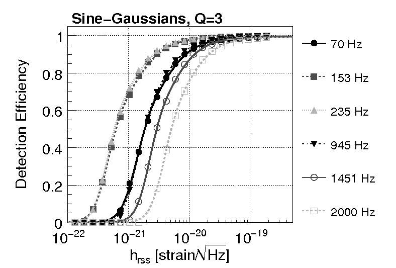
(b)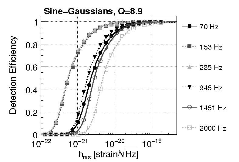
(c)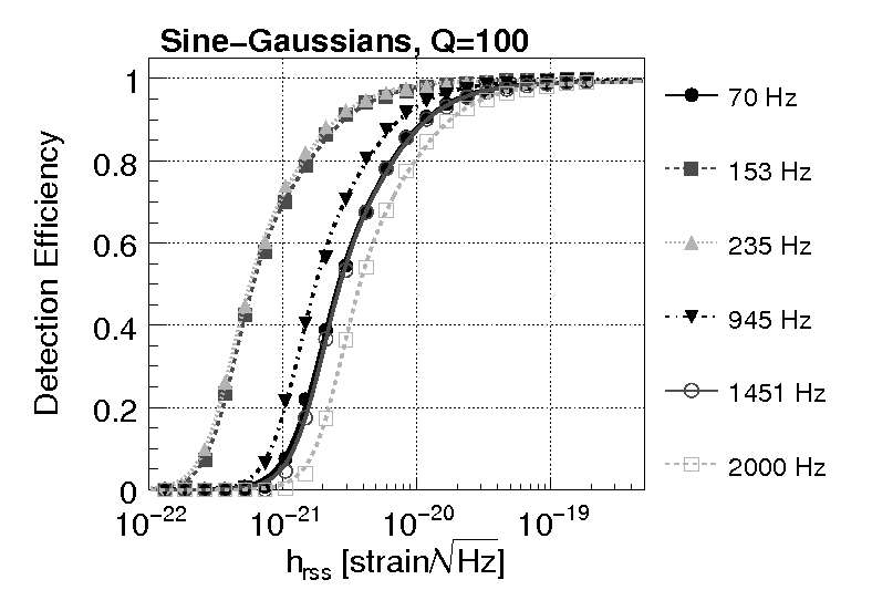
(a)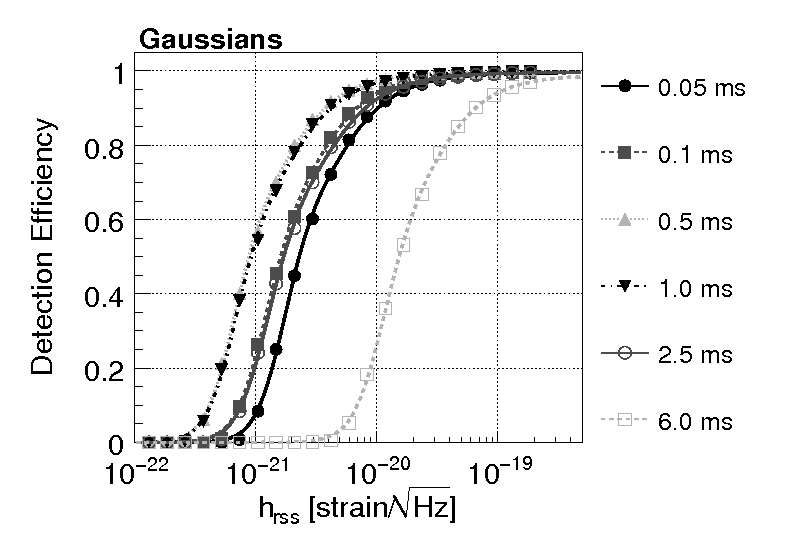
(b)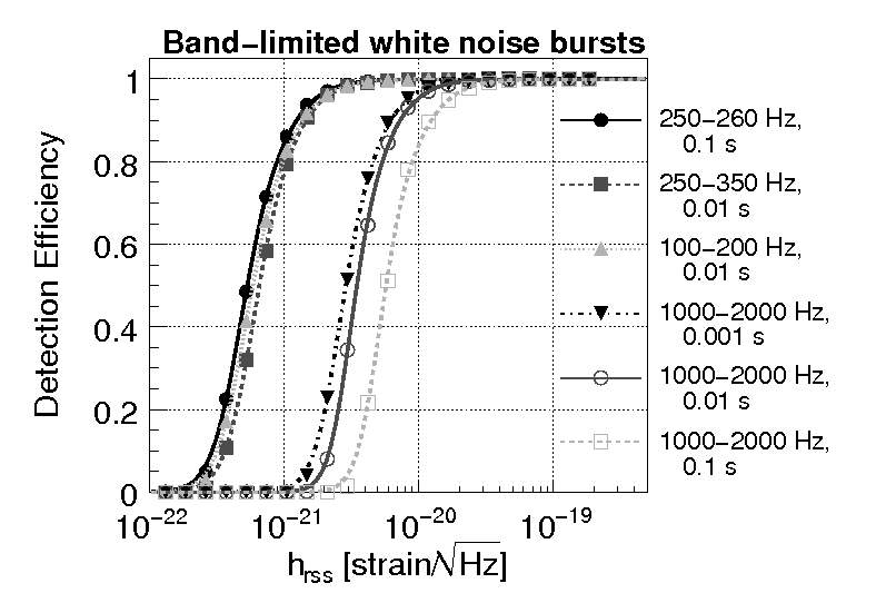
Each efficiency curve, consisting of the efficiencies determined for a given signal morphology at each of the 22 values, was fitted with an empirical four-parameter function. The efficiency curves for the logical OR combination of the three pipelines and for the combined H1H2 and H1H2L1 networks are shown for selected waveforms in Figs. 3 and 4. The values yielding 50% detection efficiency, , are shown in Tables I and II for sine-Gaussians with and for white noise bursts injected and analyzed in H1H2L1 data. The study of the efficiency for all the waveforms shows that the combination of the methods is slightly more sensitive than the best performing one, which is QPipeline for some of the sine-Gaussians, and cWB for all other waveforms considered.
| (Hz) | Combined | cWB | BN | QP | |
|---|---|---|---|---|---|
| 70 | 9 | 25.8 | 25.9 | 227.4 | 33.1 |
| 100 | 9 | 10.3 | 10.5 | 13.6 | 14.0 |
| 153 | 9 | 6.3 | 6.5 | 7.8 | 8.8 |
| 235 | 9 | 6.0 | 6.3 | 7.7 | 6.8 |
| 361 | 9 | 10.9 | 11.2 | 16.3 | 12.0 |
| 554 | 9 | 12.0 | 12.6 | 15.5 | 12.9 |
| 849 | 9 | 18.1 | 19.0 | 23.7 | 19.2 |
| 945 | 9 | 20.6 | 21.6 | 27.8 | 22.2 |
| 1053 | 9 | 23.3 | 24.8 | 33.4 | 24.1 |
| 1172 | 9 | 25.2 | 26.8 | 36.5 | 26.3 |
| 1304 | 9 | 28.7 | 30.9 | 40.8 | 29.5 |
| 1451 | 9 | 32.0 | 35.0 | 48.1 | 32.9 |
| 1615 | 9 | 35.2 | 38.2 | 51.5 | 36.3 |
| 1797 | 9 | 42.0 | 44.2 | 62.2 | 45.4 |
| 2000 | 9 | 54.5 | 55.9 | 77.6 | 68.8 |
| (Hz) | BW (Hz) | (ms) | Combined | cWB | BN | QP |
|---|---|---|---|---|---|---|
| 1000 | 1000 | 0.001 | 32.0 | 34.4 | 51.8 | 33.2 |
| 1000 | 1000 | 0.01 | 38.6 | 39.1 | 47.1 | 51.9 |
| 1000 | 1000 | 0.1 | 63.4 | 65.8 | 73.0 | 113.6 |
| 1000 | 100 | 0.01 | 22.2 | 22.6 | 30.9 | 25.9 |
| 1000 | 100 | 0.1 | 28.5 | 28.5 | 44.6 | 44.6 |
| 1000 | 10 | 0.1 | 21.5 | 21.4 | 30.8 | 44.8 |
| 100 | 100 | 0.01 | 6.5 | 6.7 | 7.5 | 9.2 |
| 100 | 100 | 0.1 | 7.9 | 7.9 | 9.9 | 14.1 |
| 100 | 10 | 0.1 | 9.1 | 9.1 | 13.7 | 12.7 |
| 250 | 100 | 0.01 | 7.3 | 7.6 | 18.6 | 8.5 |
| 250 | 100 | 0.1 | 8.8 | 8.9 | 11.6 | 13.4 |
| 250 | 10 | 0.1 | 5.9 | 5.9 | 9.0 | 17.6 |
VIII Statistical and calibration errors
The values presented in this paper have been adjusted to conservatively reflect systematic and statistical uncertainties. The dominant source of systematic uncertainty is from the amplitude measurements in the frequency domain calibration. The individual amplitude uncertainties from each interferometer can be combined into a single uncertainty by calculating a combined root-sum-square amplitude SNR and propagating the individual uncertainties assuming each error is independent. In addition, there is a small uncertainty (about 1%) introduced by converting from the frequency domain to the time domain strain series on which the analysis was actually run. There is also phase uncertainty on the order of a few degrees in each interferometer, arising both from the initial frequency domain calibration and the conversion to the time domain. However, this is not a significant concern since the phase uncertainties at all frequencies correspond to phase shifts on the order of less than half a sample duration. We therefore do not make any adjustment to the overall systematic uncertainties due to phase error. Finally, statistical uncertainties on the fit parameters (arising from the binomial errors on the efficiency measurements) affect by approximately 1.4% on average and are not much different for any particular waveform.
The frequency-domain amplitude uncertainties are added in quadrature with the other smaller uncertainties to obtain a total 1-sigma relative error for the SNR. The relative error in the is then the same as the relative error in the SNR. Thus, we adjust our sensitivity estimates by increasing the values by the reported percent uncertainties multiplied by 1.28 (to rescale from a 1-sigma fluctuation to a 90% confidence level upper limit, assuming Gaussian behavior), which amounts to 11.1% in the frequency band explored in this paper.
IX Search Results
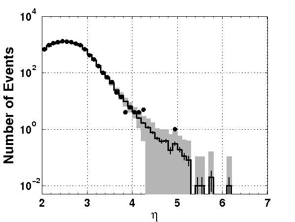
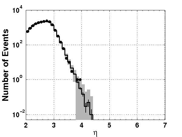
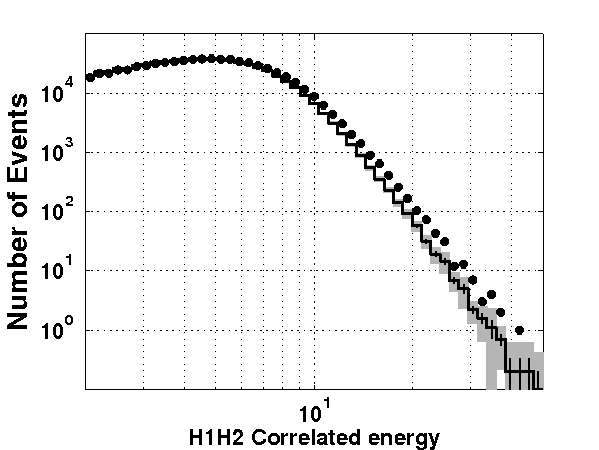
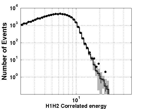
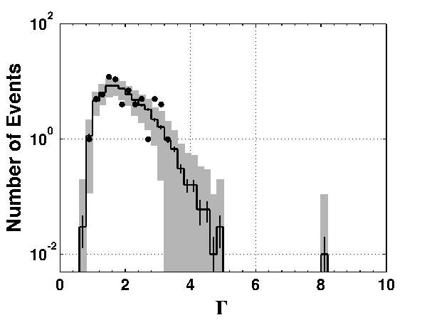
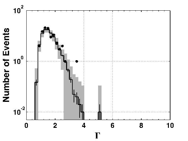
Once category 2 DQFs have been applied on the triggers produced from the unshifted (i.e. candidate sample) and time-shifted (background) data, histograms of the two populations are generated for each pipeline, interferometer network and frequency band. See for example trigger distributions for the H1H2L1 network in Figs. 5, 6, and 7. No unshifted triggers are found above threshold in the final sample for any of the three pipelines and four network configurations. We therefore have no candidate GW signals, and no follow up for possible detections is performed. We proceed to set upper limits on the rate of specific classes of GWs.
IX.1 Upper limits
Our measurements consist of the list of triggers detected by each analysis pipeline (BN, QP, cWB) in each network data set (H1H2L1, H1H2, H1L1, H2L1). BN analyzed the H1H2L1 data, QP analyzed H1H2L1 and H1H2, and cWB analyzed all four data sets. In general, the contribution to the upper limit due to a given pipeline and data set increases with both the detection efficiency of the pipeline and the livetime of the data set. Since the duty cycle of the H1L1 and H2L1 data sets is small (2.4% and 4.5% after category 3 DQFs and category 3 vetoes, vs. 37.2% and 22.5% in H1H2L1 and H1H2), and the data quality not as good, we decided a priori to not include these data sets in the upper limit calculation. We are therefore left with five analysis pipeline results: BN-H1H2L1, QP-H1H2L1, QP-H1H2, cWB-H1H2L1, and cWB-H1H2. We wish to combine these 5 results to produce a single upper limit on the rate of GW bursts of each of the morphologies tested.
We use the approach described in Sutton (2009) to combine the results of the different search detection algorithms and networks. Here we give only a brief summary of the technique.
The procedure given in Sutton (2009) is to combine the sets of triggers according to which pipeline(s) and/or network detected any given trigger. For example, in the case of two pipelines “A” and “B”, the outcome of the counting experiment is the set of three numbers , where is the number of events detected by pipeline A but not by B, is the number detected by B but not by A, and is the number detected by both. (The extension to an arbitrary number of pipelines and data sets is straightforward.) Similarly, one characterizes the sensitivity of the experiment by the probability that any given GW burst will be detected by a given combination of pipelines. We therefore compute the efficiencies , where is the fraction of GW injections that are detected by pipeline A but not by B, etc.
To set an upper limit, one must decide a priori how to rank all possible observations, so as to determine whether a given observation contains “more” or “fewer” events than some other observation . Denote the ranking function by . Once this choice is made, the actual set of unshifted events is observed, giving , and the rate upper limit at confidence level is given by
| (5) |
Here is the prior probability of observing given the true GW rate , the vector containing the livetimes of different data sets (this is a scalar if we are combining results of methods analyzing the same livetime), and the detection efficiencies . The sum is taken over all for which ; i.e., over all possible outcomes that result in “as few or fewer” events than were actually observed.
As shown in Sutton (2009), a convenient choice for the rank ordering is
| (6) |
That is, we weight the individual measurements proportionally to the corresponding efficiency . This simple procedure yields a single upper limit from the multiple measurements. From the practical point of view, it has the useful properties that the pipelines need not be independent, and that combinations of pipelines and data sets in which it is less likely for a signal to appear (relatively low ) are naturally given less weight.
Note that for the purpose of computing the upper limit on the GW, we are ignoring any background. This leads to our limits being somewhat conservative, since a non-zero background contribution to will tend to increase the estimated limit.
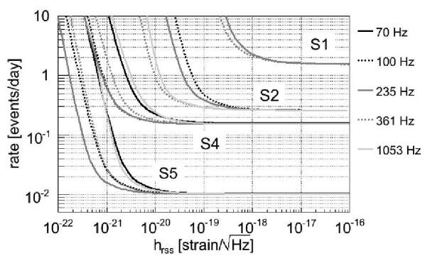
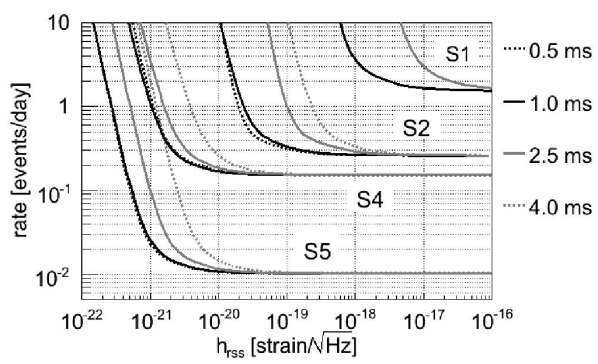
In the present search, no events were detected by any analysis pipeline, so . As shown in Sutton (2009), in this case the efficiency weighted upper limit procedure given by Eqs. (5) and (6) gives a particularly simple result: the procedure is equivalent to taking the logical OR of all five pipeline/network samples. The confidence level upper limit for zero observed events, , is given by
| (7) | |||||
| (8) |
where is the weighted average of all the efficiencies (the weight is the relative livetime) and is the total observation time. Fig. 8 shows the combined rate upper limits as a function of amplitude for selected sine-Gaussian and Gaussian GW bursts. In the limit of strong signals, goes to 224.0 days which is the union of all time analyzed for the H1H2L1 and H1H2 networks after category 3 DQFs. The rate limit thus becomes .
X Summary and Discussion
The search for unmodeled GW bursts reported in this paper is currently the most sensitive ever performed. The quality of the data and the sensitivity of the data analysis algorithms have improved since the S4 run, and the quantity of data available for analysis has increased by more than an order of magnitude. These improvements are reflected in the greater strain sensitivity (with values as low as ) and the tighter limit on the rate of bursts (less than 3.75 events per year at 90% confidence level) with large enough amplitudes to be detected reliably. The most sensitive previous search, using LIGO S4 data, achieved sensitivites as low as a few times and a rate limit of 55 events per year. We note that the IGEC network of resonant bar detectors has set a more stringent rate limit, events per year at 95% confidence level Astone et al. (2003), for GW bursts near the resonant frequencies of the bars with (see Sec. X of Abbott et al. (2005a) for the details of this comparison). A later joint observation run, IGEC-2, was a factor of 3 more sensitive but had shorter observation time Astone et al. (2007).
In order to set an astrophysical scale to the sensitivity achieved by this search, we now repeat the analysis and the examples presented for S4. Specifically, we can estimate what amount of mass converted into GW burst energy at a given distance would be strong enough to be detected by the search with 50% efficiency. Following the same steps as in Abbott et al. (2007), assuming isotropic emission and a distance of 10 kpc we find that a 153 Hz sine-Gaussian with would need solar masses, while for S4 the figure was . For a source in the Virgo galaxy cluster, approximately 16 Mpc away, the same would be produced by an energy emission of roughly , while for S4 it was .
We can also update our estimates for the detectability of two classes of astrophysical sources: core collapse supernovae and binary black-hole mergers. We consider first the core collapse supernova simulations by Ott. et al. Ott et al. (2006). In this paper gravitational waveforms were computed for three progenitor models: s11WW, m15b6 and s25WW. From S4 to S5 the astrophysical reach for the s11WW and m15b6 models improved from approximately 0.2 to 0.6 kpc while for s25WW it improved from 8 to 24 kpc. Second, we consider the binary black hole merger calculated by the Goddard numerical relativity group J. Baker, J.Centrella, D. Choi, M. Koppitz, and J. van Meter (2006). A binary system of two 10-solar-mass black holes (total ) would be detectable with 50% efficiency at a distance of roughly 4 Mpc compared to 1.4 Mpc in S4, while a system with total mass would be detectable out to 180 Mpc, compared to 60 Mpc in S4. In each case the astrophysical reach has improved by approximately a factor of 3 from S4 to S5.
At present, the analysis of the second year of S5 is well underway, including a joint analysis of data from Virgo’s VSR1 run which overlaps with the final 4.5 months of S5. Along with the potential for better sky coverage, position reconstruction and glitch rejection, the joint analysis brings with it new challenges and opportunities. Looking further ahead, the sixth LIGO science run and second Virgo science run are scheduled to start in mid 2009, with the two LIGO 4 km interferometers operating in an “enhanced” configuration that is aimed at delivering approximately a factor of two improvement in sensitivity, and comparable improvements for Virgo. Thus we will soon be able to search for GW bursts farther out into the universe.
Acknowledgements.
The authors gratefully acknowledge the support of the United States National Science Foundation for the construction and operation of the LIGO Laboratory and the Science and Technology Facilities Council of the United Kingdom, the Max-Planck-Society, and the State of Niedersachsen in Germany for support of the construction and operation of the GEO600 detector. The authors also gratefully acknowledge the support of the research by these agencies and by the Australian Research Council, the Council of Scientific and Industrial Research of India, the Istituto Nazionale di Fisica Nucleare of Italy, the Spanish Ministerio de Educación y Ciencia, the Conselleria d’Economia Hisenda i Innovació of the Govern de les Illes Balears, the Royal Society, the Scottish Funding Council, the Scottish Universities Physics Alliance, The National Aeronautics and Space Administration, the Carnegie Trust, the Leverhulme Trust, the David and Lucile Packard Foundation, the Research Corporation, and the Alfred P. Sloan Foundation. This document has been assigned LIGO Laboratory document number LIGO-P080056-v12.Appendix A Data quality flags
Data quality flags are defined by the LIGO Detector Characterization group by carefully processing information on the behavior of the instrument prior to analyzing unshifted triggers. Some are defined online, as the data are acquired, while others are formulated offline. A wide range of DQFs have been defined. The relevance of each available DQF has been evaluated and classified into categories which are used differently in the analysis, which we now describe.
Category 1 DQFs are used to define the data set processed by the search algorithms. They include out-of-science mode, the 30 seconds before loss of lock, periods when the data are corrupted and periods when test signals are injected into the detector. They also include short transients that are loud enough to significantly distort the detector response and could affect the power spectral density used for normalization by the search algorithm, such as dropouts in the calibration and photodiode saturations.
Category 2 flags are unconditional post-processing data cuts, used to define the “full” data set used to look for detection candidates. The flags are associated with unambiguous malfunctioning with a proven correlation with loud transients in the GW channel, where we understand the physical coupling mechanism. They typically only introduce a fraction of a percent of deadtime over the run. Examples include saturations in the alignment control system, glitches in the power mains, time-domain calibration anomalies, and large glitches in the thermal compensation system.
Category 3 DQFs are applied to define the “clean” data set, used to set an upper limit in the absence of a detection candidate. Any detection candidate found at a time marked with a category 3 DQF would not be immediately rejected but would be considered cautiously, with special attention to the effect of the flagged condition on detection confidence. DQF correlations with transients in the GW channels are established at the single interferometer level. Examples include the 120 s prior to lock-loss, noise in power mains, transient drops in the intensity of the light stored in the arm cavities, times when one Hanford instrument is unlocked and may negatively affect the other instrument, times with particularly poor sensitivity, and times associated with severe seismic activity, high wind speed, or hurricanes. These flags introduce up to 10% dead time.
Category 4 flags are advisory only: We have no clear evidence of a correlation to loud transients in the GW channel, but if we find a detection candidate at these times, we need to exert caution. Examples are certain data validation issues and various local events marked in the electronic logs by operators and science monitors.
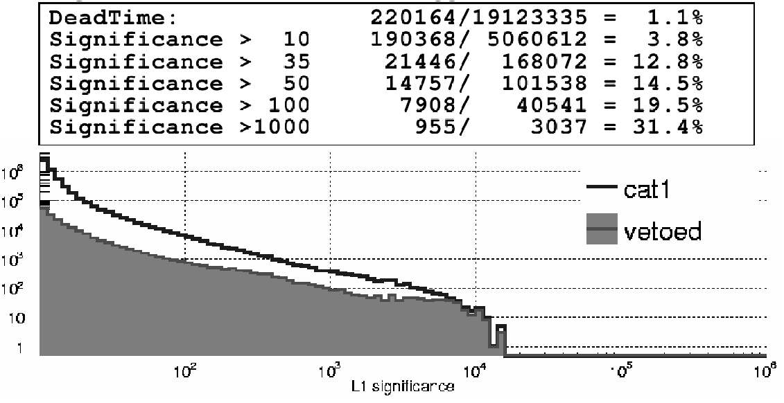
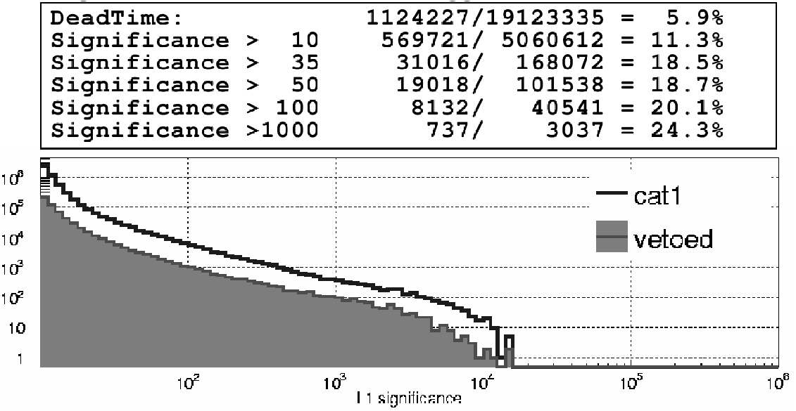
Figure 9 shows the fraction of KleineWelle triggers that are eliminated by category 2 and 3 DQFs, respectively, in the L1 interferometer, as a function of the significance of the energy excess identified by the trigger, which is evaluated assuming stationary, random noise. To ensure DQFs are independent of the presence of a true GW, we verified they are not triggered by hardware injections.
Appendix B Event-by-event vetoes
Event-by-event vetoes attempt to discard GW channel noise events by using information from the many environmental and interferometric auxiliary channels which measure non-GW degrees of freedom. Good vetoes are found by looking for situations in which a short (ms) noise transient in an auxiliary channel, identified by the KleineWelle (KW) algorithm, often coincides within a short interval (100 ms) with noise transients in the GW channel. The work, then, is in identifying useful auxiliary channels which are well correlated with noise transients in the GW data, choosing the relevant veto parameters to use, and finally establishing that the veto procedure will not systematically throw out true GWs. As for the data quality flags, vetoes are defined prior to generating triggers from unshifted data. The trigger properties used for veto studies are the KW signal energy-weighted central time and the KW statistical significance. The correlation between noise events in the GW channel and an auxiliary channel is determined by a comparison of the coincidence rate measured properly and coincidence rate formed when one of the time series has been artificially time-shifted with respect to the other. Alternatively, we can compare the number of coincidences with the number expected by chance, assuming Poisson statistics.
As for the DQFs, category 2 vetoes are defined using only a few subsets of related channels, showing the more obvious kinds of mechanisms for disturbing the interferometers – either vibrational or magnetic coupling. Furthermore, for this S5 analysis we insist that multiple (3 or more) channels from each subset be excited in coincidence before declaring a category 2 veto, to ensure that a genuine disturbance is being measured in each case. By contrast, the category 3 vetoes use a substantially larger list of channels. The aim of this latter category of veto is to produce the optimum reduction of false events for a chosen tolerable amount of livetime loss.
B.0.1 Veto effectiveness metrics
Veto efficiency is defined for a given set of triggers as the fraction vetoed by our method. We use a simple veto logic where an event is vetoed if its peak time falls within a veto window, and define the veto dead-time fraction to be the fraction of livetime flagged by all the veto windows. Assuming that real events are randomly distributed in time, dead-time fraction represents the probability of vetoing a true GW event by chance. We will refer to the flagged dead-time as the veto segments. A veto efficiency greater than the dead-time fraction indicates a correlation between the triggers and veto segments.
Under either the assumption of randomly distributed triggers, or randomly distributed dead-time, the number of events that fall within the flagged dead-time is Poisson distributed with mean value equal to the number of events times the fractional dead-time, or equivalently, the event rate times the duration of veto segments. We define the statistical significance of actually observing vetoed events as .
We must also consider the safety of a veto condition: auxiliary channels (besides the GW channel) could in principle be affected by a GW, and a veto condition derived from such a channel could systematically reject a genuine signal. Hardware signal injections imitating the passage of GWs through our detectors, performed at several pre-determined times during the run, have been used to establish under what conditions each channel is safe to use as a veto. Non-detection of a hardware injection by an auxiliary channel suggests the unconditional safety of this channel as a veto in the search, assuming that a reasonably broad selection of signal strengths and frequencies were injected. But even if hardware injections are seen in the auxiliary channels, conditions can readily be derived under which no triggers caused by the hardware injections are used as vetoes. This involves imposing conditions on the strength of the triggers and/or on the ratio of the signal strength seen in the auxiliary channel to that seen in the GW channel.
Veto safety was quantified in terms of the probability of observing N coincidence events between the auxiliary channel and hardware injections vs. the number of coincidences expected from time-shifts.
The observed concident rate is a random variable itself that
fluctuates around the true coincident rate.
In the veto analysis we use the 90% confidence upper limit
on the background coincidence rate which can be derived from the observed
coincidence rate.
This procedure makes it easier to consider a veto safe than
unsafe and the reason for this approach was to lean toward vetoing
questionable events. A total of 20 time-shifts were
performed. The analysis looped over 7 different auxiliary channel thresholds and
calculated this probability, and a probability of less than 10% caused a veto
channel at and below the given threshold to be judged unsafe. A fixed 100 ms
window between the peak time of the injection and the peak time of the
KleineWelle trigger in the auxiliary channel was used.
All channels used for category 2 vetoes were found to be safe at any threshold. Thresholds for category 3 veto channels were chosen so as to ensure that the channel was safe at that threshold and above.
B.0.2 Selection of veto conditions
For the purpose of defining conservative vetoes appropriate for applying as category 2 (before looking for GW detections), we studied environmental channels. We found that these fall into groups of channels that each veto a large number of the same events. Based on this observation, three classes of environmental channels were adopted as vetoes. For LHO these classes were 24 magnetometers and voltmeters with a KW threshold of 200 and time window of 100 ms, and 32 accelerometers and seismometers with a threshold on the KW significance of 100 and a time window of 200 ms. For LLO these were 12 magnetometers and voltmeters with a KW threshold of 200 and a time window of 100 ms. We used all of the channels that should have been sensitive to similar effects across a site, with the exception that channels known to have been malfunctioning during the time period were removed from the list.
To ensure that our vetoes are based on true environmental disturbances, a further step of voting was implemented. An event must be vetoed by three or more channels in a particular veto group in order to be discarded from the detection search. These conditions remove 0.1% from the S5 livetime.
In the more aggressive category 3 vetoes, used for cleaning up the data for an upper limit analysis, we draw from a large number of channels (about 60 interferometric channels per instrument, and 100 environmental channels per site). This task is complicated by the desire to choose optimal veto thresholds and windows, and the fact that the veto channels themselves can be highly correlated with each other so that applying one veto channel changes the incremental cost (in additional dead-time) and benefit (in additional veto efficiency) of applying another. Applying all vetoes which perform well by themselves often leads to an inefficient use of dead-time as dead-time continues to accumulate while the same noise events are vetoed over and over.
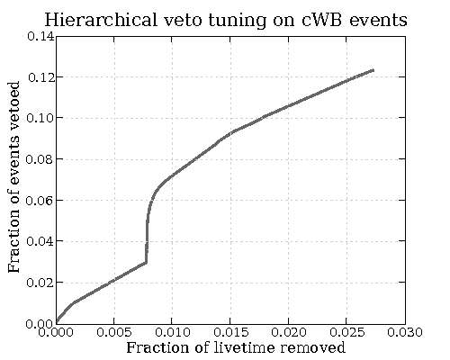
For a particular set of GW channel noise events, we adopt a “hierarchical” approach to choose the best subset of all possible veto conditions to use for a target dead-time. This amounts to finding an ordering of veto conditions (veto channel, threshold, and window) from best to worst such that the desired set of veto conditions can be made by accumulating from the top veto conditions so long as the dead-time does not exceed our limit, which is typically a few percent.
We begin with an approximately ordered list based on the performance of each veto condition (channel, window, and threshold) considered separately. Incremental veto statistics are calculated for the entire list of conditions using the available ordering. This means that for a given veto condition, statistics are no longer calculated over the entire S5 livetime, but only over the fraction of livetime that remains after all veto conditions earlier in the list have been applied. The list is then re-sorted according to the incremental performance metric and the process is repeated until further iterations yield a negligible change in ordering.
The ratio of incremental veto efficiency to incremental dead-time is used as a performance metric to sort veto conditions. This ratio gives the factor by which the rate of noise events inside the veto segments exceeds the average rate. By adopting veto conditions with the largest incremental efficiency/dead-time ratio, we maximize total efficiency for a target dead-time. We also set a threshold of probability on veto significance (not to be confused with the significance of the triggers themselves). This is particularly important for low-number statistics when large efficiency/dead-time ratios can occasionally result from a perfectly random process.
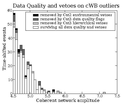
Vetoes were optimized over several different sets of GW channel noise events including low-threshold H1H2L1 coherent WaveBurst time-shifted events, H1H2 coherent WaveBurst playground events, as well as QPipeline and KleineWelle single-interferometer triggers. For example, the effect of data quality flags and event-by-event vetoes on the sample of coherent WaveBurst time-shifted events is shown in Fig. 10. Our final list of veto segments to exclude from the S5 analysis is generated from the union of these individually-tuned lists.
Appendix C The BlockNormal Burst Search Algorithm
C.1 Overview
The BlockNormal analysis pipeline follows a similar logic to the S4 burst analysis Abbott et al. (2007) by looking for bursts that are both coincident and correlated. The BlockNormal pipeline uses a change-point analysis to identify coincident transient events of high significance in each detector’s data. The subsequent waveform correlation test is the same as that used in the S4 analysis.
A unique feature of the BlockNormal analysis is that it can be run on uncalibrated time series data—neither the change point analysis nor the correlation test are sensitive to the overall normalization of the data.
C.2 Data conditioning
The BlockNormal search operated on the frequency range 80 to 2048 Hz. To avoid potential issues with the additional processing and filtering used to create calibrated data, and to be immune to corrections in the calibration procedure, the analysis was run on the uncalibrated GW channel from the LIGO interferometers.
The data conditioning began with notch filters to suppress out-of-band (below 80 Hz or above 2048 Hz) spectral features such as low-lying calibration lines, the strong 60 Hz power-line feature and violin mode harmonics just above 2048 Hz. The time-series data were then down-sampled to 4096 Hz to suppress high-frequency noise. The power-line harmonics in each band were removed using Kalman filters Kalman (1960); Finn and Mukherjee (2001). The large amount of power at low frequencies in the uncalibrated GW channel was suppressed with a highpass filter designed with the Parks-McClellan algorithm.
Because the BlockNormal method is purely a time-domain statistic, the interferometer data must be divided into frequency bands to achieve a degree of frequency resolution on the bursts. For this analysis, 12 frequency bands approximately 150 Hz in bandwidth spanned the range from 80 Hz to 2048 Hz (see Table 3). There are gaps between some bands to avoid the significant non-stationary noise from the violin modes of the mirror suspension wires.
| Lower Bound (Hz) | Upper Bound (Hz) | Bandwidth (Hz) |
| 80 | 192 | 112 |
| 192 | 320 | 128 |
| 362 | 518 | 156 |
| 518 | 674 | 156 |
| 710 | 864 | 154 |
| 864 | 1018 | 154 |
| 1060 | 1212 | 152 |
| 1212 | 1364 | 152 |
| 1408 | 1558 | 150 |
| 1558 | 1708 | 150 |
| 1756 | 1902 | 146 |
| 1902 | 2048 | 146 |
The division into the twelve frequency bands was done using a basebanding procedure. Any calibration lines within the band were removed by low-order regression filtering against the calibration line injection channel data. A final whitening filter of modest order was applied in each band to satisfy the BlockNormal statistic’s assumption of Gaussianity in the background noise. The data conditioning procedures also had to minimize mixing noise characteristics between different time periods for the change-point analysis, and thus could not rely on predictive filtering.
C.3 Change-point analysis
The BlockNormal algorithm uses a Bayesian statistic termed to perform a change-point analysis using the noise characteristics of time-series data. For an interval of time-series samples , this statistic measures the statistical likelihood (at each sample within that interval) that the data prior to that point are more consistent with a different Gaussian-distributed (or normal) noise source than are the data following that point. It is defined as
where
| (10) | |||
| (11) | |||
| (12) |
The quantity is a constant proportional to , where is the prior probability, R the desired rate of blocks, and the sample rate. In fact each interval is searched for all change-points where exceeds a threshold value , where is implemented as a number times . The sub-intervals between change-points are termed “blocks”. The statistical significance of each such block is based on its “excess power” defined as
| (13) |
where the block has mean and variance against a background of mean and variance . Events were selected by requiring the negative-log-likelihood of (termed ) to exceed a threshold. Here
| (14) |
where
| (15) |
The variance-weighted time centroid, , of each event of samples of amplitude and time was calculated:
| (16) |
The calibrated band-limited strain energy of each event was estimated using the frequency-averaged response over that band:
| (17) |
The BlockNormal algorithm was applied separately to the data in each frequency band (Table 3) to select candidate GW burst events. The burst event generation was done on relatively long-duration epochs (up to 1200 s) of continuous data to provide the best measure of the background noise characteristics.
Prior to the network coincidence step, events within each frequency band that are nearly adjacent were clustered into composite events. Then, events between adjacent frequency bands whose time centroids were close were clustered into composite multiband events. All events were then characterized by their frequency coverage. For composite events, the effective time centroid was the energy-weighted average of the time centroid of the constituent events. The band-limited energy for composite events was simply the sum of the per-event energies. The central frequency for events in a single band was estimated by the average frequency of that band. For multi-band events, the energy-weighted average of these central frequencies was used.
C.4 Network coincidence
The signals from actual GW bursts in the LIGO interferometers should be separated in time by no more than the maximum transit time ( ms) for GW between the Hanford and Livingston sites. For the co-located interferometers at Hanford, there should be no time separation. The separation observed in the reconstructed events is larger due to limited time resolution, phase-delays in filtering, etc. For a candidate trigger, the time difference between candidate events in each pair of interferometers, , was required to fall within a fixed coincidence window, , for that pair of interferometers. This coincidence window had to be much broader than the transit time to account for limited time resolution and skewing of the time distributions from differential antenna response to and waveforms.
The signals from actual GW bursts should also have similar strain amplitude (and hence statistical significance) in each interferometer. We derived a measure of coincident significance from the excess power significance in each candidate event in the trigger. This measure must correct for the lower significance for GW signals in the shorter H2 interferometer (as compared to the H1 interferometer) as well as the fluctuation of the relative GW signal strengths at the two LIGO sites due to modulation from the antenna factors. The chosen metric for coincident significance, termed “combined power” or , was defined as
| (18) |
This formulation was found to have the best performance in optimizing sensitivity to GW burst signals as a function of the background trigger rate.
The coincidence procedure first identified events from each of the three detectors that had overlapping frequency coverage. These events then had to have time centroids whose difference was less than ms. Such time-coincidence events were retained as GW burst triggers if their combined power was above a threshold of 22.
C.5 Network correlation
The signals from GW bursts in each interferometer result from the same parent waveforms, and thus should have a large correlation sample-by-sample (after correction for propagation delay). The cross-correlation statistic reported by the CorrPower Cadonati (2004) package is the maximum of the average correlation confidence of pair-wise correlation tests. It is positive-definite. Larger values denote greater statistical certainty of coherence. The CorrPower package was run on the list of candidate trigger times produced in the coincidence step. It retrieved the full time-series data from each interferometer around that time, calibrated the data, and calculated the cross-correlation statistic. For the three LIGO interferometers, cuts were also made on the three pair-wise correlation tests.
Additional selection criteria took advantage of the special relationship for GW signals from the co-located interferometers H1 and H2. One was the signed correlation factor between the H1 and H2 interferometers from the CorrPower processing, termed . For triggers from GW bursts, this correlation factor should be positive. For triggers from a background of random coincidences, there should be an equal number of positive and negative correlation factors. Also, since the H1 and H2 interferometers receive the same GW signal, the ratio of to should be close to one for a true GW burst. In contrast, for triggers from a random background this ratio will be centered around one-half. This arises because the H2 interferometer is approximately half as sensitive as H1, so signals of the same statistical significance (near the threshold) will have only one-half the amplitude in H2 as they do in H1. To simplify thresholding, the absolute value of the logarithm of the ratio was calculated for later use.
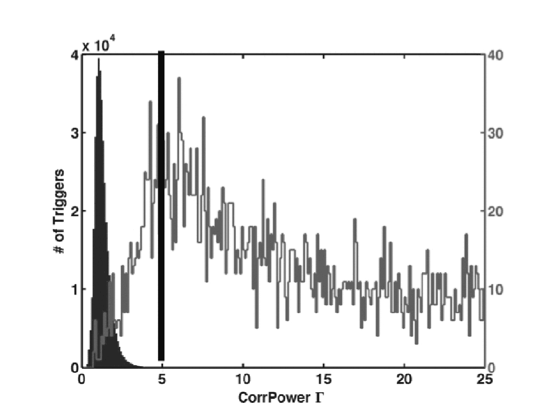
The choices of tuning parameters are described in Table 4. Figure 11 illustrates an example of plots used to tune the figures of merit for the H1H2L1 network.
| H1H2L1 Network |
|---|
| for Hz |
| for Hz |
| , , |
Appendix D The QPipeline burst search algorithm
D.1 Overview
QPipeline is an analysis pipeline for the detection of GW bursts in data from interferometric gravitational wave detectors Chatterji (2005). It is based on the Q transform Chatterji et al. (2004), a multi-resolution time-frequency transform that projects the data under test onto the space of bisquare-windowed complex exponentials characterized by central time , central frequency , and quality factor :
| (19) |
where the bisquare window is
| (20) |
with
| (21) |
The bisquare window is a close approximation to a Gaussian window in frequency space; the QPipeline is effectively a templated matched filter search Wainstein and Zubakov (1962) for signals that are Gaussian enveloped sinusoids in the whitened signal space.
D.2 Data conditioning
Before applying the Q transform, the data are first whitened by zero-phase linear predictive filtering Makhoul (1975); Chatterji (2005). In linear predictive whitening, the th sample of a discrete data sequence is assumed to be well modeled by a linear combination of the previous samples:
| (22) |
The resulting whitened data stream is the prediction error sequence that remains after selecting the coefficients to minimize the error in the least-squares sense.
The prediction error length is taken to be equal to the length of the longest basis function under test, which is approximately 1 second. This ensures that the data are uncorrelated on the time scales of the analysis.
In order to avoid introducing phase errors between detectors, a modified zero-phase whitening filter is constructed by zero-padding the initial filter, converting to the frequency domain, and discarding all phase information.
D.3 Measurement basis
The space of Gaussian enveloped complex exponentials is an over-complete basis of waveforms, whose duration and bandwidth have the minimum possible time-frequency uncertainty, , where . As a result, they provide the tightest possible constraints on the time-frequency area of a signal, maximizing the measured signal to noise ratio (SNR) and minimizing the probability that false triggers are coincident in time and frequency between multiple detectors.
In practice, the Q transform is evaluated only for a finite number of basis functions, which are more commonly referred to as templates or tiles. These templates are selected to cover a targeted region of signal space, and are spaced such that the fractional signal energy loss due to the mismatch , , and between an arbitrary basis function and the nearest measurement template,
| (23) |
is no larger than . This naturally leads to a tiling of the signal space that is logarithmic in , logarithmic in frequency, and linear in time.
For this search, the QPipeline was applied to search the space of sinusoidal Gaussians with central frequency from 48 Hz to 2048 Hz, and with from to .
D.4 Trigger generation
The statistical significance of Q transform projections are given by their normalized energy , defined as the ratio of squared projection magnitude to the mean squared projection magnitude of other templates with the same central frequency and . For the case of ideal white noise, is exponentially distributed and is related to the matched filter SNR quantity Wainstein and Zubakov (1962) by the relation
| (24) |
The Q transform is applied to the whitened data and normalized energies are computed for each measurement template as a function of time. Templates with statistically significant signal content are then identified by applying a threshold on the normalized energy. Finally, since a single event may potentially produce multiple overlapping triggers due to the overlap between measurement templates, only the most significant of overlapping templates are reported as triggers.
Clustering of nearby triggers is not used in evaluating the significance of events. As a result, the detectability of GW burst signals depends on their maximum projection onto the space of Gaussian enveloped sinusoids.
D.5 Coherence
For this search, the QPipeline took advantage of the co-located nature of the two LIGO Hanford detectors to form two linear combinations of the data streams from the two detectors. This coherent analysis makes use of correlations in the data to distinguish true GW signals from instrumental glitches.
D.5.1 Coherent signal stream
The first combination is the coherent signal stream, , a frequency dependent weighted sum of the data from the Hanford detectors which maximizes the effective SNR. The weighting is inversely proportional to the noise power spectral density, :
| (25) |
The resulting combination is treated as the output of a new hybrid, “coherent” detector. Under the assumption that the power spectral density is approximately flat across the window bandwidth, applying the Q transform to this data stream leads to a coherent energy value, , which takes the following form:
| (26) |
where , , and are functions of , , and , and the asterisk denotes complex conjugation. The last term represents the contribution of the cross-term, and is conceptually similar to a frequency domain representation of a cross-correlation of the H1 and H2 data streams.
The energy expected in the coherent data stream if there were no correlations in the data can be characterized by the “incoherent” terms in Eq. (26):
| (27) |
The coherent and incoherent energies can then be normalized in the manner of Eq. (24):
| (28) | |||||
| (29) |
The correlation between the detectors can then be measured by the correlated energy, , given by
| (30) |
D.5.2 Null stream
The second combination is the difference between the calibrated data from the two detectors, known as the null stream, and is defined as
| (31) |
By subtracting the co-located streams, any true gravitational wave signal should be canceled. The resulting combination is treated as the output of a new hybrid “” detector, which shows significant energy content in the presence of instrumental glitches but does not respond to gravitational waves. Glitches are identified by thresholding on the corresponding normalized “null energy”, , calculated in an analogous manner to .
Signal tiles found to be in coincidence with significant null stream tiles are vetoed as instrumental glitches, and are not considered as candidate events. The threshold on can be expressed as
| (32) |
where is chosen to limit the veto rate in Gaussian noise to per 2048 tiles and is a parameter corresponding to the allowed tolerance in calibration uncertainty. This is an energy factor, and corresponds to an amplitude calibration uncertainty of approximately 22 percent.
We expect that highly energetic instrumental glitches could leak energy into adjacent time-frequency bins, so the veto coincidence requirement between signal and null streams is scaled to give more-significant null stream tiles more area of veto influence in time-frequency space:
| (33) |
| (34) |
where and are the central time and frequency of a tile, and are the duration and bandwidth of a tile, and the inflated null stream tile duration and bandwidth are defined as:
| (35) |
| (36) |
D.6 Coincidence
Coherent triggers from the two LIGO Hanford detectors were also tested for time-frequency coincidence with triggers from the LIGO Livingston detector using the following criteria, where is the speed of light travel time of 10 ms between the two LIGO sites:
| (37) |
| (38) |
Coincidence between the LIGO Hanford and Livingston sites is not a requirement for detection, even if detectors at both sites are operational. The final trigger set is the union of triggers from the coherent H1H2 trigger set and the coincident H1H2L1 trigger set. The additional requirement of coincidence permits a lower threshold, and therefore greater detection efficiency, for the H1H2L1 data set.
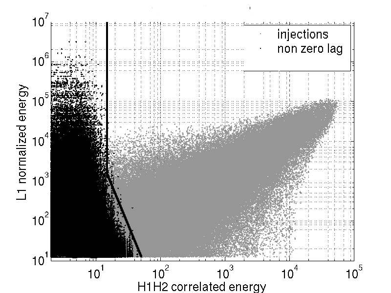
The choices of tuning parameters are described in Table 5. Figure 12 an example scatter plot used to tune the figures of merit for the H1H2L1 network.
| H1H2L1 Network | |||
| for Hz | |||
| for Hz | |||
| H1H2 Network | |||
| for Hz | |||
| for Hz | |||
Appendix E The coherent WaveBurst search algorithm
E.1 Overview
Coherent WaveBurst (cWB) is an analysis pipeline for the detection and reconstruction of GW burst signals from a network of detectors. The reconstructed gravitational waveform that best describes the response of the network is used to compute the maximum likelihood ratio of the putative GW signal, which forms the main detection statistic for the search. In effect, cWB is equivalent to a matched filter search with a very large template bank representing all possible time-domain signals with short duration.
The cWB pipeline is divided into three main stages: the generation of coherent triggers, the reconstruction of the GW signal and the computation of the maximum likelihood ratio, and a post-production stage where additional detection cuts are applied. By using weighted coherent combinations of the data streams, cWB is not limited by the least sensitive detector in the network. The waveform reconstruction allows various physical properties of the signal to be estimated, including the sky location of the source. The coherent approach also allows for other statistics to be constructed, such as the null stream and coherent energy, to distinguish genuine GW signals from environmental and instrumental artifacts.
E.2 Data conditioning and time-frequency decomposition
The cWB analysis is performed in the wavelet domain. A discrete Meyer wavelet transformation is applied to the sampled detector output to produce a discrete wavelet series , where is the time index, is the scale index and is the detector index. An important property of Meyer wavelets is that they form an orthonormal basis that allow for the construction of wavelet filters with small spectral leakage Klimenko et al. (2008). Wavelet series give a time-scale representation of data where each wavelet scale can be associated with a certain frequency band of the initial time series. Therefore a wavelet time-scale spectrum can be displayed as a time-frequency (TF) scalogram, where the scale is replaced with the central frequency of the band. The time series sampling rate and the scale number determine the time resolution at this scale. The frequency resolution is defined as and determines the data bandwidth at the scale . The time-frequency resolution defines the tiling of the TF plane. The individual tiles (pixels) represent data samples in the wavelet domain. In the cWB pipeline a uniform tiling is used , where is the wavelet decomposition depth), which is obtained with the Meyer packet transformation Vidakovic (1999). In this case the TF resolution is the same for all wavelet scales. For optimal localization of the GW energy in the TF plane, the cWB analysis is performed at six different frequency resolutions: 8, 16, 32, 64, 128 and 256 Hz.
Before the coherent analysis is performed, two data conditioning algorithms are applied to the data in the wavelet domain: a linear prediction error (LPE) filter and a wavelet estimator of the power spectral density . LPE filters are used to remove “predictable” components from an input data series. In the cWB pipeline they are constructed individually for each wavelet layer and remove such components in the data as power line harmonics and violin-mode lines. A more detailed description of the LPE filters can be found elsewhere Klimenko et al. (2005, 2008). The wavelet estimator of the one-sided power spectral density associated with each wavelet layer is
| (39) |
where is the variance of the detector noise. In the analysis we assume that the detector noise is Gaussian and quasi-stationary. The variance estimator may vary with time and therefore it is calculated for each sample in the wavelet layer: . The estimation of the noise variance is performed on data segments of length 60 seconds, with 40 seconds overlap. Linear interpolation is used between two measurements to obtain .
E.3 Coherent triggers
The first step in the analysis is to identify segments of data that may contain a signal. The triggers are evaluated using the whitened data vector
| (40) |
The sampled detector amplitudes in the wavelet domain take into account the time delays due to the time-of-flight between the detectors, which in turn depend on the source coordinates and . Coherent triggers are generated for the entire network by maximizing the norm over the entire sky for each time-frequency location . To do this, the sky is divided into square degree patches and the quantity is calculated for each patch from the delayed detector amplitudes . By selecting clusters of pixels with the above some threshold, one can identify coherent triggers in the time-frequency plane. The data pixels selected by this procedure are then used to reconstruct the GW signal and compute the maximum likelihood statistic.
E.4 Maximum likelihood ratio functional
For the case of Gaussian quasi-stationary noise, the likelihood that data is purely instrumental noise is proportional to , while the likelihood that a GW signal is present is proportional to . The ratio of these likelihoods can be used as a detection statistic. Here defines a noise weighted inner product, which for detectors with uncorrelated noise can be written in the wavelet domain as
| (41) |
where time and frequency indices run over some time-frequency area selected for the analysis. The coherent WaveBurst pipeline defines as twice the (log) likelihood ratio, and treats it as a functional in Klimenko et al. (2005):
| (42) |
where are the detector responses (Eq. 2). The network sensitivity is characterized by the noise-scaled antenna pattern vectors and :
| (43) |
Since the detector responses are independent of rotation by an arbitrary polarization angle in the wave frame, it is convenient to perform calculations in the dominant polarization frame (DPF) Klimenko et al. (2005). In this frame the antenna pattern vectors and are orthogonal to each other:
| (44) |
and we refer to them as and respectively. The corresponding solutions for the GW waveforms, and , are found by variation of the likelihood functional (Eq. (42)) that can be written as the sum of two terms, , where
| (45) | |||
| (46) |
The estimators of the GW waveforms for a particular sky location are then the solutions of the equations and :
| (47) | |||
| (48) |
Note, the norms and characterize the network sensitivity to the and polarizations respectively. The maximum likelihood ratio statistic for sky location is calculated by substituting the solution for into . The result can be written as
| (49) |
where the matrix is the projection constructed from the components of the unit vectors and along the directions of the and respectively:
| (50) |
The kernel of the projection is the signal plane defined by these two vectors. The null space of the projection defines the reconstructed detector noise which is referred to as the null stream.
The projection matrix is invariant with respect to the rotation in the signal plane where any two orthogonal unit vectors can be used for construction of the . Therefore one can select vectors and such that and
| (51) |
The unit vector defines the vector
| (52) |
whose components are estimators of the noise-scaled detector responses .
E.5 Regulators
In principle the likelihood approach outlined above can be used for the reconstruction of the GW waveforms and calculation of the maximum likelihood statistic. In practice the formal solutions (47), (48) need to be regularized by constraints that account for the way the network responds to a generic GW signal Klimenko et al. (2005). For example, the network may be insensitive to GW signals with a particular sky location or polarization, resulting in an ill-posed inversion problem. These problems are addressed by using regulators and sky-dependent penalty factors.
A classical example of a singular inversion problem is a network of aligned detectors where the detector responses are identical. In this case the algorithm can be constrained to search for one unknown function rather than for the two GW polarizations and , which span a larger parameter space. Note that in this case , Eq. (48) is ill-conditioned and the solution for the waveform cannot be found. Regulators are important not only for aligned detectors, but also for networks of misaligned detectors, for example, the LIGO and Virgo network. Depending on the source location, the network can be much less sensitive to the second GW component () and the waveform may not be reconstructable from the noisy data.
In the coherent WaveBurst analysis we introduce a regulator by modifying the norm of the vector:
| (53) |
where is a tunable parameter. For example, if , the second GW component is entirely suppressed and the regulator corresponds to the “hard constraint” described in Ref. Klimenko et al. (2005). In this case the unit vector (see Eq. (51)) is pointing along the direction. In the cWB analysis the parameter is chosen to be
| (54) |
This regulator is more stringent for weak events which are generated by the pipeline at much higher rate than the loud events.
The introduction of the regulator creates an obvious problem for the construction of the projection matrix. Namely, the vector and the corresponding vector obtained by rotation of and in the signal plane are not unit vectors if . To fix this problem we re-normalize the vector to unity and use it for calculation of the maximum likelihood ratio and other coherent statistics.
E.6 Coherent statistics
When the detector noise is Gaussian and stationary, the maximum likelihood is the only statistic required for detection and selection of the GW events. In this case the false alarm and the false dismissal probabilities are controlled by the threshold on which is an estimator of the total SNR detected by the network. However, the real data are contaminated with instrumental and environmental artifacts and additional selection cuts should be applied to separate them from genuine GW signals Klimenko et al. (2008). In the coherent WaveBurst method these selection cuts are based on coherent statistics constructed from the elements of the likelihood and the null matrices. The diagonal terms of the matrix describe the reconstructed normalized incoherent energy. The sum of the off-diagonal terms is the coherent energy detected by the network.
The next step is to optimize the solution over the sky. Often, depending on the network configuration, the reconstruction of source coordinates is ambiguous. For example, for two separated detectors the relative time delay that yields maximum correlation between the data streams corresponds to an annulus on the sky. In this case, an “optimal” source location is selected, where the reconstructed detector responses are the most consistent with the output detector data streams. To properly account for the directional sensitivity of the network the optimization over sky locations has to be more than a simple maximization of . In the cWB analysis the statistic that is maximized has the form
| (55) |
where is the penalty factor and is the network correlation coefficient. and are defined below in terms of the matrix and the diagonal matrices and which describe the normalized energy in the detectors, and the normalized reconstructed signal energy (see Eq. (52)), with
| (56) |
Ideally, the reconstructed signal energy in each detector should not significantly exceed the energy . This requirement can be enforced by the constraint
| (57) |
for each detector in the network. These constraints can be applied during the signal reconstruction by way of Lagrange multipliers in the variational analysis, however this greatly increases the computational complexity of the algorithm. A simpler alternative is to introduce a penalty factor that penalizes sky locations violating the constraint equation (57):
| (58) |
In addition to serving as a penalty factor in the position reconstruction, the ratio of reconstructed and detector energy were also used as a post-production cut. Events with were discarded, as were events with large values of the network energy disbalance
| (59) |
and the H1-H2 energy disbalance
| (60) |
The latter cut was found to be particularly effective at rejecting correlated glitches in the two Hanford interferometers.
The network correlation coefficient is also used to weight the overall likelihood for each sky location. It is defined as
| (61) |
where is the sum of all elements in the null matrix
| (62) |
which represents the normalized energy of the reconstructed noise. Usually for glitches little coherent energy is detected and the reconstructed detector responses are inconsistent with the detector output, which results in a large value for the null energy. In addition to helping select the optimal sky location, the correlation coefficients are used for a signal consistency test based on the comparison of the null energy and the coherent energy.
The coherent terms of the likelihood matrix can be also used to calculate the correlation coefficients
| (63) |
which represent Pearson’s correlation coefficients in the case of aligned detectors. We use the coefficients to construct the reduced coherent energy
| (64) |
Combined with the network correlation coefficient and the number of detectors in the network, , it yields a quantity which we call the coherent network amplitude,
| (65) |
Figure 13 shows the – distribution of the background events (see Sec. VI) and simulated GW events (see Sec. VII) for the L1H1H2 network. Loud background events due to detector glitches with low values of the network correlation coefficient are rejected by a threshold on . Relatively weak background events are rejected by a threshold on . Table 6 describes the full set of tuning parameters for cWB.
| H1H2L1 Network |
| , |
| for Hz, up to Dec 12 2005 03:19:29 |
| or after Oct 25 2006 09:34:17 |
| for Hz, between Dec 12 2005 03:19:29 |
| and Oct 25 2006 09:34:17 |
| for Hz |
| , |
| H1H2 Network |
| , |
| for Hz |
| for Hz, up to Jul 17 2006 11:50:37 |
| for Hz, after Jul 17 2006 11:50:37 |
| , |
| H1L1 Network |
| , |
| for Hz, up to Oct 07 2006 08:58:06 |
| for Hz, after Oct 07 2006 08:58:06 |
| for Hz |
| H2L1 Network |
| , |
| for Hz, up to Mar 28 2006 04:23:06 |
| or after Oct 28 2006 11:54:46 |
| for Hz, between Mar 28 2006 04:23:06 |
| and Oct 28 2006 11:54:46 |
| for Hz |
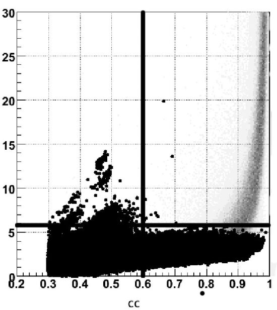
References
- Abbott et al. (2009a) B. Abbott et al. (LIGO Scientific Collaboration), Rep. Prog. Phys. 72, 076901 (2009a).
- H. Grote (2008) (for the LIGO Scientific Collaboration) H. Grote (for the LIGO Scientific Collaboration), Class. Quantum Grav. 25, 114043 (2008).
- Acernese et al. (2006) F. Acernese et al., Class. Quantum Grav. 23, 563 (2006).
- Culter and Thorne (2002) C. Culter and K. Thorne, in General Relativity and Gravitation, edited by N. T. Bishop and D. M. Sunil (2002), p. 72, eprint arXiv:gr-qc/0204090.
- Blanchet (2006) L. Blanchet, Living Reviews in Relativity 9, 4 (2006).
- Jaranowski and Schutz (1998) A. Jaranowski, P. Krolak and B. Schutz, Phys. Rev. D 58, 063001 (1998).
- J. Baker, J.Centrella, D. Choi, M. Koppitz, and J. van Meter (2006) J. Baker, J.Centrella, D. Choi, M. Koppitz, and J. van Meter, Phys. Rev. D 73, 104002 (2006).
- Ott et al. (2004) C. D. Ott, A. Burrows, E. Livne, and R. Walder, Astrophys. J. 600, 834 (2004).
- Ott et al. (2006) C. D. Ott, A. Burrows, L. Dessart, and E. Livne, Phys. Rev. Lett. 96, 201102 (2006).
- C. D. Ott, H. Dimmelmeier, A. Marek, H-T Janka, B. Zink, I. Hawke and E. Schnetter (2007) C. D. Ott, H. Dimmelmeier, A. Marek, H-T Janka, B. Zink, I. Hawke and E. Schnetter, Class. Quantum Grav. 24, S139 (2007).
- Ott (2009) C. D. Ott, Class. Quantum Grav. 26, 063001 (2009).
- Abbott et al. (2008a) B. Abbott et al. (LIGO Scientific Collaboration), Phys. Rev. D 77, 062002 (2008a).
- Abbott et al. (2009b) B. Abbott et al. (LIGO Scientific Collaboration) (2009b), submitted to Phys. Rev. D, eprint arXiv:0904.4910 [gr-qc].
- Abbott et al. (2005a) B. Abbott et al. (LIGO Scientific Collaboration), Phys. Rev. D 72, 062001 (2005a).
- Abbott et al. (2005b) B. Abbott et al. (LIGO Scientific Collaboration and TAMA Collaboration), Phys. Rev. D 72, 122004 (2005b).
- Abbott et al. (2006) B. Abbott et al. (LIGO Scientific Collaboration), Class. Quantum Grav. 23, 200511 (2006).
- Abbott et al. (2007) B. Abbott et al. (LIGO Scientific Collaboration), Class. Quantum Grav. 24, 5343 (2007).
- Abbott et al. (2008b) B. Abbott et al. (LIGO Scientific Collaboration), Class. Quantum Grav. 25, 245008 (2008b).
- Hughey (2009) B. Hughey, LIGO DCC number T0900468-V1 (2009).
- Sigg et al. (2006) D. Sigg et al., Class. Quantum Grav. 23, S51 (2006).
- Waldman et al. (2006) S. Waldman et al., Class. Quantum Grav. 23, S653 (2006).
- R. Adhikari, G. Gonzalez, M. Landry and B. O’Reilly (2003) R. Adhikari, G. Gonzalez, M. Landry and B. O’Reilly, Class. Quantum Grav. 20, S903 (2003).
- Abbott et al. (2004) B. Abbott et al. (LIGO Scientific Collaboration), Phys. Rev. D 69, 102001 (2004).
- Blackburn et al. (2005) L. Blackburn et al., LIGO-G050158-00-Z (2005), URL http://www.ligo.caltech.edu/docs/G/G050158-00.
- Shantanu Desai, Sam Finn, John McNabb, Amber Stuver, Tiffany Summerscales and Keith Thorne (2004) Shantanu Desai, Sam Finn, John McNabb, Amber Stuver, Tiffany Summerscales and Keith Thorne, Class. Quantum Grav. 21, S1705 (2004).
- Chatterji (2005) S. K. Chatterji, Ph.D. thesis, Massachusetts Institute of Technology (2005).
- Chatterji et al. (2004) S. Chatterji, L. Blackburn, G. Martin, and E. Katsavounidis, Class. Quantum Grav. 21, S1809 (2004).
- Klimenko et al. (2008) S. Klimenko, I. Yakushin, A. Mercer, and G. Mitselmakher, Class. Quantum Grav. 25, 114029 (2008).
- Anderson et al. (2001) W. G. Anderson, P. R. Brady, J. D. Creighton, and É. É. Flanagan, Phys. Rev. D 63, 042003 (2001).
- Chatterji et al. (2006) S. Chatterji, A. Lazzarini, L. Stein, P. J. Sutton, A. Searle, and M. Tinto, Phys. Rev. D 74, 082005 (2006).
- Sutton (2009) P. J. Sutton (2009), eprint arXiv:0905.4089 [physics.data-an].
- Astone et al. (2003) P. Astone et al., Phys. Rev. D 68, 022001 (2003).
- Astone et al. (2007) P. Astone et al., Phys. Rev. D 76, 102001 (2007).
- Kalman (1960) R. E. Kalman, Trans. ASME Ser. D. J. Basic Eng. 82, 35 (1960).
- Finn and Mukherjee (2001) L. S. Finn and S. Mukherjee, Phys. Rev. D 63, 062004 (2001), erratum-ibid.D67:109902,2003.
- Cadonati (2004) L. Cadonati, Class. Quantum Grav. 21, S1695 (2004).
- Wainstein and Zubakov (1962) L. Wainstein and V. Zubakov, Extraction of signals from noise (Prentice-Hall, Englewood Cliffs, U.S.A., 1962).
- Makhoul (1975) J. Makhoul, Proc. IEEE 63 (1975).
- Vidakovic (1999) B. Vidakovic, Statistical Modeling by Wavelets (Wiley, New York, 1999).
- Klimenko et al. (2005) S. Klimenko, S. Mohanty, M. Rakhmanov, and G. Mitselmakher, Phys. Rev. D 72, 122002 (2005).