Fast Frame-Based Image Deconvolution Using
Variable
Splitting and Constrained Optimization
Abstract
We propose a new fast algorithm for solving one of the standard formulations of frame-based image deconvolution: an unconstrained optimization problem, involving an data-fidelity term and a non-smooth regularizer. Our approach is based on using variable splitting to obtain an equivalent constrained optimization formulation, which is then addressed with an augmented Lagrangian method. The resulting algorithm efficiently uses a regularized version of the Hessian of the data fidelity term, thus exploits second order information. Experiments on a set of image deblurring benchmark problems show that our algorithm is clearly faster than previous state-of-the-art methods.
1 Introduction
1.1 Problem Formulation
The standard model in image deblurring assumes that the noisy blurred observed version , of an original image , was obtained via
where is the matrix representation of a convolution and is Gaussian white noise. In frame-based deblurring/deconvolution, the unknown image is expressed as , where the columns of matrix are the elements of a frame, such as a wavelet orthonormal basis or a redundant dictionary [6], [7], [8], [11], [13], [14]. The coefficients of this representation are then estimated, under one of the well-known sparsity inducing regularizers, typically the norm, leading to the optimization problem
| (1) |
in (1), is the regularizer, which is usually convex but nonsmooth, and is the regularization parameter [7]. This formulation is called the synthesis approach [12], since it is based on the synthesis equation . In the last decade, a considerable amount of research has been devoted to designing efficient algorithms for solving (1). This interest has been further stimulated by the recent emergence of compressive sensing (CS) [5], [9], since CS reconstruction can be formulated as (1) [17], [24].
1.2 Previous Algorithms
In most practical problems (including CS), matrix (and even or ) cannot be stored explicitly and it is highly impractical to access portions (lines/columns or blocks) of it. These facts preclude most off-the-shelf optimization algorithms from being directly used and has stimulated the development of special purpose methods. These methods operate under the constraint and (and their transposes) can only be used to form matrix-vector products, since these products can be performed efficiently using the FFT and fast wavelet transforms.
Arguably, the standard algorithm for solving (1) is the so-called iterative shrinkage/thresholding (IST), which can be derived from different viewpoints: expectation-maximization [13], majorization-minimization [8], [14], forward-backward operator splitting [7], [16]. A key ingredient of IST is the so-called shrinkage/thresholding function associated to , , defined as
| (2) |
An excellent coverage of these functions, also known as Moreau proximal maps, can be found in [7].
The fact that IST tends to be slow, in particular when is poorly conditioned, has stimulated some recent research aimed at obtaining faster variants. The recent two-step IST (TwIST) algorithm [3], in which each iteration uses the two previous iterates (rather than only the previous one, as in IST), was shown to be considerably faster than IST on various deconvolution problems. Another two-step variant of IST, named fast IST algorithm (FISTA), was recently proposed and also shown to be faster than IST [2]. A recent strategy to obtaining faster variants of IST consists in using more aggressive choices of step size in each iteration. This is the case in the SpaRSA (sparse reconstruction by separable approximation) framework [21], [22], which was also shown to clearly outperform standard IST.
1.3 Proposed Approach
The approach proposed in this paper is based on variable splitting. The idea is to split the variable into a pair of variables and , each to serve as the argument of each of the two functions in (1), and then minimize the sum of the two functions under the constraint that the two variables have to be equal, thus making the problems equivalent. This rationale has been recently used in the split-Bregman method [15], which was proposed to address constrained optimization formulations for solving inverse problems. In this paper, we exploit a different splitting to attack problem (1), arguably the most classical formulation for frame-based regularization of linear inverse problems [6], [7].
The constrained optimization problem produced by the splitting procedure is addressed using an augmented Lagrangian (AL) algorithm [18]. AL was shown to be equivalent to the Bregman iterative methods [19], [23]. We adopt the AL perspective, rather than the Bregman view, as it is a more standard optimization tool. We show that by exploiting the fact that is a frame, the resulting algorithm solves (1) much faster than the previous state-of-the-art methods FISTA [2], TwIST [3], and SpaRSA [22].
The speed of the proposed algorithm may be justified by the fact that it uses (a regularized version of) the Hessian of the data fidelity term, , while the above mentioned algorithms essentially only use gradient information. Although, as referred earlier, this matrix can not be formed, we show that if is a tight frame and a convolution, our algorithm can use it in an efficient way.
2 Basic Tools
2.1 Variable Splitting
Consider an unconstrained optimization problem in which the objective is the sum of two functions:
| (3) |
Variable splitting (VS) is a simple procedure in which a new variable is introduced to serve as the argument of , under the constraint that . In other words, the constrained problem
| (4) |
is equivalent to (3), since in the feasible set , the objective function in (4) coincides with that in (3).
VS was used in [20] to derive a fast algorithm for total-variation based restoration. VS was also used in [4] to handle problems where instead of the single regularizer in (1), there is a linear combination of two (or more) regularizers: . In [4] and [20], the constrained problem (4) is attacked by a quadratic penalty approach, i.e., by solving
| (5) |
by alternating minimization with respect to and , while slowly increasing to force the solution of (5) to approach that of (4). The idea is that each step of this alternating minimization may be much easier than the original unconstrained problem (3). The drawback is that as increases, the intermediate minimization problems become increasingly ill-conditioned, thus causing numerical problems [18].
2.2 Augmented Lagrangian
Consider a linear equality constrained optimization problem
| (6) |
where and . The so-called augmented Lagrangian function for this problem is defined as
| (7) |
where is a vector of Lagrange multipliers and is called the AL penalty parameter [18]. The AL algorithm iterates between minimizing with respect to , keeping fixed, and updating .
- Algorithm AL
-
1.
Set , choose , , and .
-
2.
repeat
-
3.
-
4.
-
5.
-
6.
until stopping criterion is satisfied.
It is possible (in some cases recommended) to update the value of at each iteration [18], [1] (Chap. 9). However, unlike in the quadratic penalty method, it is not necessary to take to infinity to guarantee that the AL converges to the solution of the constrained problem (6). In this paper, we will consider only the case of fixed .
After a straightforward manipulation, the terms added to in (see (7)) can be written as a single quadratic term, leading to the following alternative form for the AL algorithm:
- Algorithm AL (version 2)
-
1.
Set , choose , , and .
-
2.
repeat
-
3.
-
4.
-
5.
-
6.
until stopping criterion is satisfied.
This form of the AL algorithm makes clear its equivalence with the Bregman iterative method, as given in [23].
2.3 AL for Variable Splitting and Its Convergence
Problem (4) can be written in the form (6) with , , , and . With these definitions in place, Steps 3 and 4 of the AL algorithm (version 2) can be written as follows
| (8) |
| (9) |
The minimization problem (8) is clearly non-trivial: in general, it involves non-separable quadratic and possibly non-smooth terms. A natural approach is to use a non-linear block-Gauss-Seidel (NLBGS) technique, in which (8) is solved by alternating minimization with respect to and , while keeping the other variable fixed. Remarkably, it has been shown that the AL algorithm converges, even if the exact solution of (8) is replaced with a single NLBGS step [10, Theorem 8] (see also [19]). The resulting algorithm is as follows.
- Algorithm Alternating Split AL
-
1.
Set , choose , , , and .
-
2.
repeat
-
3.
-
4.
-
5.
-
6.
-
7.
until stopping criterion is satisfied.
Problem (1) has the form (3) where is quadratic, thus Step 3 consist in solving a linear system of equations. We will return to the particular form of this system in the next section. With , a regularizer, Step 4 corresponds to applying a shrinkage/thresholding function, that is, usually a computationally inexpensive operation.
3 Proposed Method
3.1 Constrained Optimization Formulation and Algorithm
Performing the VS on problem (1) yields the following constrained formulation:
| (10) |
This VS decouples the quadratic non-separable term from the non-quadratic term , to deal with the non-separability of the quadratic data term. In contrast, split-Bregman methods use a splitting to avoid non-separability of the regularizer.
Problem (10) has the form (4), with , , , and . Applying this translation table to the Alternating Split AL algorithm presented Section 2.3, we obtain the following algorithm.
- Algorithm Split AL Shrinkage Algorithm
-
1.
Set , choose , , , and .
-
2.
repeat
-
3.
-
4.
-
5.
-
6.
-
7.
-
8.
-
9.
until stopping criterion is satisfied.
Since Step 4 is a strictly convex quadratic problem, its solution is unique and given by
| (11) |
In the next subsection, we show how can be efficiently computed. Note that is a regularized (by the addition of ) version of the Hessian of .
3.2 Computing
Assume that is a normalized tight (Parseval) frame, i.e., (although possibly ), and that is the matrix representation of a convolution, i.e., products by or can be computed in the Fourier domain, with cost via the FFT.
The assumptions in the previous paragraph will enable us to compute the matrix inversion in (11), even if it is not feasible to explicitly form matrix . Using the Sherman -Morrison- Woodbury inversion formula, (11) becomes
| (12) | |||||
where . Furthermore, since is the matrix representation of a convolution, (12) can be written as
| (13) |
where
| (14) |
and are the matrix representations of the forward and inverse discrete Fourier transform (DFT), and is a diagonal matrix containing the DFT of the convolution represented by . Notice that the product by corresponds to applying a filter in the DFT domain, which can be done using FFT algorithms with cost. Notice also that can be precomputed. When the products by and are direct and inverse tight frame transforms for which fast algorithms exist, the leading cost of each application of (13) will be either or the cost of these frame transforms (usually also ).
Finally, the complete algorithm, which we term SALSA (split augmented Lagrangian shrinkage algorithm) is as follows.
- Algorithm SALSA
-
1.
Initialization: set ; choose , , , ;
-
2.
compute
-
3.
compute
-
4.
repeat
-
5.
-
6.
-
7.
-
8.
-
9.
-
10.
-
11.
-
12.
until stopping criterion is satisfied.
4 Experiments
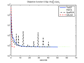
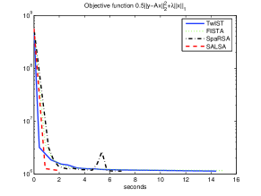
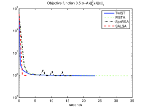
We consider five standard image deconvolution benchmark problems [13], summarized in Table 1, all on the well-known Cameraman image. The regularizer is , thus is a soft threshold. In all the experiments, is a redundant Haar wavelet frame, with levels, and the blur operator is applied via the FFT. The regularization parameter in each case was hand tuned for best improvement in SNR. The value of for fastest convergence was found to differ in each case, but a good rule of thumb, used in all the experiments, is . We compare SALSA with current state of the art methods: TwIST [3], SpaRSA [22], and FISTA [2], in terms of the time taken to reach the same value of the objective function. Table 2 shows the CPU times taken by each of the algorithms in each of the experiments. Figure 1 shows the plots of the objective function , evolving over time, in experiments , B, and A.
| Experiment | blur kernel | |
|---|---|---|
| 1 | uniform | |
| 2A | Gaussian | 2 |
| 2B | Gaussian | 8 |
| 3A | 2 | |
| 3B | 8 |
| Experiment | TwIST | SpARSA | FISTA | SALSA |
|---|---|---|---|---|
| 1 | 50.2969 | 42.0469 | 64.2344 | 4.000 |
| 2A | 30.7656 | 40.6094 | 61.7031 | 4.03125 |
| 2B | 14.4063 | 6.92188 | 15.0781 | 1.9375 |
| 3A | 23.5313 | 17.0156 | 33.7969 | 2.60938 |
| 3B | 8.1875 | 6.17188 | 18.0781 | 1.89063 |


5 Conclusions
We have proposed a fast algorithm for frame-based image deconvolution, based on variable splitting and solving the constrained optimization problem through an augmented Lagrangian scheme. Experimental results with regularization show that our new algorithm outperforms existing state-of-the-art methods in terms of computation time, by a considerable factor. Future work includes the application of SALSA to other inverse problems, namely compressed sensing and reconstruction with missing samples.
References
- [1] M. Bazaraa, H. Sherali, and C. Shetty, Nonlinear Programming: Theory and Algorithms, John Wiley & Sons, New York, 1993.
- [2] A. Beck and M. Teboulle, “A fast iterative shrinkage-thresholding algorithm for linear inverse problems”, SIAM Journal on Imaging Sciences, vol. 2, pp. 183–202, 2009.
- [3] J. Bioucas-Dias and M. Figueiredo, “A new TwIST: two-step iterative shrinkage/thresholding algorithms for image restoration”, IEEE Transactions on Image Processing, vol. 16, no. 12, pp. 2992-3004, 2007.
- [4] J. Bioucas-Dias and M. Figueiredo, “An iterative algorithm for linear inverse problems with compound regularizers”, IEEE International Conference on Image Processing - ICIP’2008, San Diego, CA, USA, 2008.
- [5] E. Candès, J. Romberg, and T. Tao. “Robust uncertainty principles: Exact signal reconstruction from highly incomplete frequency information,” IEEE Transactions on Information Theory, vol. 52, pp. 489–509, 2006.
- [6] C. Chaux, P. Combettes, J.-C. Pesquet, V. Wajs, “A variational formulation for frame-based inverse problems”, Inverse Problems, vol. 23, pp. 1495–1518, 2007.
- [7] P. Combettes and V. Wajs, “Signal recovery by proximal forward-backward splitting,” SIAM Journal on Multiscale Modeling & Simulation, vol. 4, pp. 1168–1200, 2005.
- [8] I. Daubechies, M. De Friese, and C. De Mol. “An iterative thresholding algorithm for linear inverse problems with a sparsity constraint.” Communications in Pure and Applied Mathematics, vol. 57, pp. 1413–1457, 2004.
- [9] D. Donoho. “Compressed sensing,” IEEE Transactions on Information Theory, vol. 52, pp. 1289–1306, 2006.
- [10] J. Eckstein and D. Bertsekas, “On the Douglas- Rachford splitting method and the proximal point algorithm for maximal monotone operators”, Mathematical Programming, vol. 5, pp. 293 -318, 1992.
- [11] M. Elad, B. Matalon, and M. Zibulevsky, “Image denoising with shrinkage and redundant representations”, Proceedings of the IEEE Computer Society Conference on Computer Vision and Pattern Recognition – CVPR’2006, New York, 2006.
- [12] M. Elad, P. Milanfar, and R. Rubinstein, “Analysis versus synthesis in signal priors”, Inverse Problems, vol. 23, pp. 947–968, 2007.
- [13] M. Figueiredo and R. Nowak. “An EM algorithm for wavelet-based image restoration.” IEEE Transactions on Image Processing, vol. 12, pp. 906–916, 2003.
- [14] M. Figueiredo and R. Nowak. “A bound optimization approach to wavelet-based image deconvolution”, Proceedings of the IEEE International Conference on Image Processing – ICIP’2005, Genoa, Italy, 2005.
- [15] T. Goldstein and S. Osher, “The split Bregman algorithm for regularized problems”, Technical Report 08-29, Computational and Applied Mathematics, University of California, Los Angeles, 2008.
- [16] T. Hale, W. Yin, Y. Zhang, “A fixed-point continuation method for -regularized minimization with applications to compressed sensing.” TR07-07, Department of Computational and Applied Mathematics, Rice University, 2007.
- [17] J. Haupt and R. Nowak. “Signal reconstruction from noisy random projections,” IEEE Transactions on Information Theory, vol. 52, pp. 4036–4048, 2006.
- [18] J. Nocedal, S. J. Wright. Numerical Optimization, 2nd Edition, Springer, 2006.
- [19] S. Setzer, “Split Bregman algorithm, Douglas-Rachford splitting, and frame shrinkage”, Proceedings of the Second International Conference on Scale Space Methods and Variational Methods in Computer Vision 2009, LNCS, Springer, 2009 (accepted).
- [20] Y. Wang, J. Yang, W. Yin, and Y. Zhang, “A new alternating minimization algorithm for total variation image reconstruction”, SIAM Journal on Imaging Sciences, vol. 1, pp. 248–272, 2008.
- [21] S. Wright, R. Nowak, M. Figueiredo, “Sparse reconstruction by separable approximation , Proceedings of the IEEE International Conference on Acoustics, Speech, and Signal Processing ICASSP 2008, Las Vegas, NV, USA, 2008.
- [22] S. Wright, R. Nowak, M. Figueiredo, “Sparse reconstruction by separable approximation , IEEE Transactions on Signal Processing, 2009 (to appear).
- [23] W. Yin, S. Osher, D. Goldfarb, and J. Darbon, “Bregman iterative algorithms for minimization with applications to compressed sensing”, SIAM Journal on Imaging Science, vol. 1, pp. 143–168, 2008.
- [24] C. Zhu, “Stable recovery of sparse signals via regularized minimization”, IEEE Transactions on Information Theory, vol. 54, pp. 3364–3367, 2008.