Parameter free scaling relation for nonequilibrium growth processes
Abstract
We discuss a parameter free scaling relation that yields a complete data collapse for large classes of nonequilibrium growth processes. We illustrate the power of this new scaling relation through various growth models, as for example the competitive growth model RD/RDSR (random deposition/random deposition with surface diffusion) and the RSOS (restricted solid-on-solid) model with different nearest-neighbor height differences, as well as through a new deposition model with temperature dependent diffusion. The new scaling relation is compared to the familiar Family-Vicsek relation and the limitations of the latter are highlighted.
pacs:
05.20.-y,64.60.Ht,68.35.Ct,05.70.NpThe study of growing interfaces has been a very active field for many years Mea93 ; Hal95 ; Bar95 . Many studies focus on the technologically relevant growth of thin films or nanostructures, but growing interfaces are also encountered in various other physical, chemical, or biological systems, ranging from bacterial growth to diffusion fronts. Over the years important insights into the behavior of nonequilibrium growth processes have been gained through the study of simple model systems that capture the most important aspects of real experimental systems Kru97 ; Kru95 .
In their seminal work, Edwards and Wilkinson investigated surface growth phenomena generated by particle sedimentation under the influence of gravity 1982SE . They proposed to describe this process in () dimensions by the following stochastic equation of motion for the surface height , now called the Edwards-Wilkinson (EW) equation,
| (1) |
where is the diffusion constant (surface tension), whereas is a Gaussian white noise with zero mean and covariance . Since Eq. 1 is linear, it can be solved exactly by Fourier transformations 1982SE ; Hal95 ; Kru97 . Later, Family 1986FF discussed the random deposition (RD) and random deposition with surface relaxation (RDSR) processes. RD 1986FF ; Bar95 is one of the simplest surface growth processes. In this lattice model particles drop from randomly chosen sites over the surface and stick directly on the top of the selected surface site. Since there is no surface diffusion, the independently growing columns yield an uncorrelated and never-saturated surface. The RDSR process is realized by adding surface diffusion which allows particles just deposited on the surface to jump to the neighboring site with lowest height. This diffusion step smoothes the surface and limits the maximum interface width , defined at deposition time as the standard deviation of the surface height from its mean value : Starting from an initially flat surface, RDSR yields at very early times, with (we assume here that one layer is deposited per unit time), a surface growing in the same way as for the RD process since no (or only very few) diffusion steps occur in that regime. For the width increases as a power law of time with a growth exponent before entering a saturation regime after a crossover time , see Fig. 1. Both the saturation width and the crossover time are powers of the substrate size :
| (2) |
where is the roughness exponent and is the dynamical exponent, with . In his study Family noticed that the scaling exponents obtained through numerical simulations of the RDSR process agree with those obtained from the solution of the EW equation. The dependence of the growing interface on the substrate size is summarized in the celebrated Family-Vicsek scaling relation 1985FF
| (3) |
Combining this with the relations given in (2), we see that this scaling relation mainly consists in shifting the crossover points for the different system sizes to a common point with the new coordinates and . It is worth noting that the Family-Vicsek relation neglects the RD regime at early times and exclusively focuses on the two regimes connected by the crossover point at .

The scaling (2) and (3) is generic for growing interfaces and has been verified analytically, numerically, and experimentally in a large variety of systems. Various universality classes have been identified which differ by the values of the scaling exponents. Thus the RDSR process belongs to the Edwards-Wilkinson universality class with the exponents and for a one-dimensional substrate. The RD process is in an universality class of its own which for a d=1 substrate is characterized by the values and . Other well known universality classes, directly related to technologically relevant growth processes, are the Kardar-Parisi-Zhang (KPZ) Kar86 and the conserved KPZ universality classes Wol90 ; Sar91 .
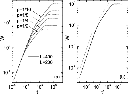
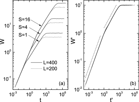
In recent years the study of nonequilibrium growth systems has shifted to more complex cases as for example competitive growth models, see e.g. Hor01 ; Hor01a ; Cha02 ; Hor03 ; Kol04 ; Mur04 ; Bra05 ; Iru05 ; Hor06 ; Rei06 ; Oli06 ; Kol06 . In a competitive growth model one considers a mixture of two different deposition processes where one of them takes place with probability whereas the other takes place with probability . One example is the RD/RDSR model Hor01 where the deposition happens according to the RDSR rules with probability and to the RD rules with probability . Whereas for and only one of the processes is realized, for general values of the mixture of the two processes leads to a crossover between the two regimes where the crossover time and width depend on the value of (see Fig. 2a). A similar dependence on system parameters is also observed in the RSOS model Kim89 which exhibits a crossover from the RD regime to the important KPZ universality class. In this model new particles are incorporated into the growing surface only if the height differences between the deposition site and its neighboring sites remain smaller than some maximum height . As discussed in Chi04 and shown in Fig. 3a, the crossover time and width depend on the value of .
In simple growth processes the random deposition regime is restricted to very early times. This is fundamentally different in more complex systems where the initial regime can extend over very large times Hor01 ; Hor01a ; Cha02 ; Hor03 ; Kol04 ; Mur04 ; Bra05 ; Iru05 ; Hor06 ; Rei06 ; Oli06 ; Kol06 ; Chi04 . As already mentioned, the Family-Vicsek scaling relation (3) assigns a new set of coordinates to the second crossover point. This does however not yield a complete data collapse for growth processes with two crossover points if one considers systems of different sizes. For the competitive growth models some phenomenological scaling relations have been proposed in the past, but these modified scaling relations also only allow a partial collapse of the different curves Hor01 ; Kol04 ; Bra05 ; Kol06 .
However, a scaling relation leading to a complete data collapse of all curves obtained for different system sizes and different values of the system parameters can indeed be obtained for any growth system that exhibits two different crossover points. This data collapse is achieved in a two-step process. First we translate all curves in a log-log plot such that the first crossover point is now located at the origin. This is achieved by plotting as a function of . In the second step we rescale both axes by the common scale factor such that in the log-log plot the second crossover point is fixed at the rescaled width . This isotropic rescaling, which conserves the slope of the region between the two crossover points, makes that the length of the line connecting the two crossover points is the same for all curves, and a complete data collapse, encompassing all three regimes, follows. Our proposed scaling relation can be cast in the following equation:
| (4) |
where is a scaling function. Introducing , we can rewrite this as
| (5) |
with a new scaling function . As shown in Fig. 2 and 3 for the RD/RDSR and RSOS processes, the proposed scaling relation yields a complete data collapse for different system sizes and different values of the system parameters. This perfect scaling behavior should be compared with the incomplete scaling proposed in the literature Hor01 ; Kol04 ; Bra05 ; Kol06 .
Obviously, the scaling relation (5) is of universal use in growth systems with two crossover points and replaces the Family-Vicsek relation in these systems. This class of systems encompasses competitive growth models, but also the simple growth systems, for which the Family-Vicsek relation has been proposed originally, belong to this class. It is also worth noting that the properties of the different models only enter in our relation (5) implicitly through the dependence of the positions of the crossover points on the different system parameters.


We can also state the new scaling relation in an alternative way which makes the difference to the Family-Vicsek relation more transparent. Indeed, a complete collapse can also be achieved when first moving the second crossover point to the origin in a log-log plot, yielding the relation
| (6) |
or
| (7) |
where and are again scaling functions. This scaling relation is completely equivalent to the first one, only the scales are shifted. In fact, the relation (7) allows a direct comparison with the Family-Vicsek relation (3): recalling that the scaling behaviors of and are given by the relations (2), we immediately see that we recover the Family-Vicsek relation by setting . This nicely shows that it is the isotropic rescaling in the log-log plot by the factor that ultimately is responsible for the success of the new scaling relation.
Competitive growth models have the peculiar feature that at every deposition one has to decide which of the two deposition rules is followed by the newly added particle. We propose in the following a deposition model with similar features as the competitive growth models, but where the competition is intrinsic and governed by the value of the substrate temperature. This is a much more realistic situation, especially since in the growth of thin films and nanostructures the substrate temperature is an important parameter that shapes to a large extend the morphology of growing structures Jen99 .
The deposition model discussed in the following is based on Family’s original RDSR process 1986FF and differs from this model by the diffusion step. In the RDSR process a particle deposited on the surface is allowed to jump to one of the neighboring sites if this site has a lower height than the site of deposition. In our model we assign an energy to the column where is the height of that column at time . The constant can be thought to be the gravitation constant. Starting from an initially flat substrate, particles are deposited on randomly chosen sites and then allowed to diffuse locally after deposition. For a diffusion step taking place at time , we select one of the neighboring sites at random and accept the jump with the temperature and time dependent (Metropolis like) probability
In the following we choose units thus that where is the Boltzmann constant.
In contrast to the original RDSR model, we have in the present model a non-vanishing probability that a deposited particle jumps to a neighboring site with a higher height than the deposition site. We assume this jump to be thermally activated and to depend on the temperature of the substrate. As we discuss elsewhere Chou09 , the substrate temperature is a parameter that allows the study of novel properties of growing interfaces.
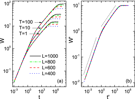
In Fig. 4a we show the temporal evolution of the width for various temperatures and system sizes. As for the RDSR process one distinguishes three regimes separated by two crossover points: a RD regime, followed by a EW regime, with a final crossover to the saturation regime. In contrast to the RDSR process, the random deposition process is not confined to the very early time regime but can extend to larger times. In fact, the crossover time between the random deposition and the EW regimes is shifted to higher values for increasing temperatures and diverges in the limit of infinite temperatures. Of special interest is that the surface widths shown in Fig. 4a can be directly obtained from the Edwards-Wilkinson equation (1) for a system of size with a temperature dependent diffusion constant. For example, for the temperatures shown in Fig. 4a, the values of are: , , and .

We first check in Fig. 4b that also for the present model the scaling relation (5) yields the full data collapse. Due to the simplicity of the model, we can obtain the full information on the location of the two crossover points Chou09 . In this way we find that, as usual, only the crossover to the saturation regime depends on the system size. In addition, the coordinates of both crossover points display a linear dependence on the substrate temperature. Taking these observations into account, we can rewrite the scaling relation (5) in the form
| (8) |
where and , with and , whereas is the roughnes exponent of the EW universality class. Eq. (8) directly reveals for our model the dependence of the generalized scaling relation on the system size and on the temperature.
In conclusion, we have presented in this letter a parameter free scaling relation that yields a complete data collapse for large classes of nonequilibrium growth processes with two crossover points. Examples include all simple growth processes as well as more complex growing interfaces as encountered for example in competitive growth systems. A deposition model with temperature dependent diffusion allows us to discuss the dependence of the scaling relation on the relevant system parameters.
References
- (1) P. Meakin, Phys. Rep. 235, 189 (1993).
- (2) T. Halpin-Healy and Y.-C. Zhang, Phys. Rep. 254, 215 (1995).
- (3) A.-L. Barábasi and H. E. Stanley, Fractal Concepts in Surface Growth (Cambridge University Press, Cambridge, 1995).
- (4) J. Krug, Advances in Physics 46, 139 (1997).
- (5) J. Krug, in Scale Invariance, Interfaces, and Non-Equilibrium Dynamics, edited by A. McKane et al. (Plenum, New York, 1995), p. 25.
- (6) S. F. Edwards and D. R. Wilkinson, Proc. R. Soc. Lond. A 381, 17 (1982).
- (7) F. Family, J. Phys. A 19, L441 (1986).
- (8) F. Family and T. Vicsek, J. Phys. A 18, L75 (1985).
- (9) M. Kardar, G. Parisi, and Y. Zhang, Phys. Rev. Lett. 56, 889 (1986).
- (10) D. E. Wolf and J. Villain, Europhys. Lett. 13, 389 (1990).
- (11) S. Das Sarma and P. Tamborenea, Phys. Rev. Lett. 66, 325 (1991).
- (12) C. M. Horowitz, R. A. Monetti, and E. V. Albano, Phys. Rev. E 63, 066132 (2001).
- (13) C. M. Horowitz and E. V. Albano, J. Phys. A 34, 357 (2001).
- (14) A. Chame and F. D. A. Aaro Reis, Phys. Rev. E 66, 051104 (2002).
- (15) C. M. Horowitz and E. V. Albano, Eur. Phys. J. B 31, 563 (2003).
- (16) A. Kolakowska, M. A. Novotny, and P. S. Verma, Phys. Rev. E 70, 051602 (2004).
- (17) D. Muraca, L. A. Braunstein, and R. C. Buceta, Phys. Rev. E 69, 065103(R) (2004).
- (18) L. A. Braunstein and C.-H. Lam, Phys. Rev. E 72, 026128 (2005).
- (19) I. Irurzun, C. M. Horowitz, and E. V. Albano, Phys. Rev. E 72, 036116 (2005).
- (20) C. M. Horowitz and E. V. Albano, Phys. Rev. E 73, 031111 (2006).
- (21) F. D. A. Aaro Reis, Phys. Rev. E 73, 021605 (2006).
- (22) T. J. Oliveira, K. Dechoum, J. A. Redinz, and F. D. A. Aaro Reis, Phys. Rev. E 74, 011604 (2006).
- (23) A. Kolakowska, M. A. Novotny, and P. S. Verma, Phys. Rev. E 73, 011603 (2006).
- (24) J. M. Kim and J. M. Kosterlitz, Phys. Rev. Lett. 62, 2289 (1989).
- (25) C.-C. Chien, N.-N. Pang, and W.-J. Tzeng, Phys. Rev. E 70, 021602 (2004).
- (26) P. Jensen, Rev. Mod. Phys. 71, 1695 (1999).
- (27) Y.-L. Chou, M. Pleimling, and R. K. P. Zia, in preparation.