Damage Spreading in Spatial and Small-world Random Boolean Networks

Abstract

The study of the response of complex dynamical social, biological, or technological networks to external perturbations has numerous applications. Random Boolean Networks (RBNs) are commonly used a simple generic model for certain dynamics of complex systems. Traditionally, RBNs are interconnected randomly and without considering any spatial extension and arrangement of the links and nodes. However, most real-world networks are spatially extended and arranged with regular, power-law, small-world, or other non-random connections. Here we explore the RBN network topology between extreme local connections, random small-world, and pure random networks, and study the damage spreading with small perturbations. We find that spatially local connections change the scaling of the relevant component at very low connectivities ($\bar{K}\ll 1$) and that the critical connectivity of stability $K_{s}$ changes compared to random networks. At higher $\bar{K}$, this scaling remains unchanged. We also show that the relevant component of spatially local networks scales with a power-law as the system size N increases, but with a different exponent for local and small-world networks. The scaling behaviors are obtained by finite-size scaling. We further investigate the wiring cost of the networks. From an engineering perspective, our new findings provide the key design trade-offs between damage spreading (robustness), the network’s wiring cost, and the network’s communication characteristics.

I Introduction

The robustness against failures, the wiring cost, and the communication characteristics are key measures of most complex, finite-size real-world networks. For example, the electrical power grid needs to be robust against a variety of failures, minimize the wiring cost, and minimize the transmission losses. Similarly, the neural circuitry in the human brain requires efficient signal transmission and robustness against damage while being constrained in volume.

In this letter, we use random Boolean networks (RBNs) as a simple model to study the (1) robustness, i.e., the damage spreading, (2) the wiring cost, and (3) the communication characteristics as a function of different network topologies (local, small-world, random), different connectivities $\bar{K}$, and different network sizes $N$. More generally speaking, this allows us to answer the question of how much and what type of interconnectivity a complex network—in our case RBNs—needs in order to satisfy given restrictions on the robustness against certain types of failure, the (wiring) cost, and the (communication) efficiency. The work presented here extends previous work by Rohlf et al. ROHLF_PRL2007 to new network topologies, which are more biologically plausible, such as for example small-world topologies.

RBNs were originally introduced by Kauffman as simplified models of gene regulation networks Kauffman69 ; Kauffman93 . In its simplest form, an RBN is discrete dynamical system, also called $NK$ network (or model), composed of $N$ automata (or nodes), each of which receives inputs from $K$ (either exact or average) randomly chosen other automata. Each automaton is a Boolean variable with two possible states: $\{0,1\}$, and the dynamics is such that

$${\bf F}:\{0,1\}^{N}\mapsto\{0,1\}^{N},$$ (1)

where ${\bf F}=(f_{1},...,f_{i},...,f_{N})$, and each $f_{i}$ is represented by a look-up table of $K_{i}$ inputs randomly chosen from the set of $N$ automata. Initially, $K_{i}$ neighbors and a look-table are assigned to each automaton at random.

$$f_{i}:\{0,1\}^{K_{i}}\mapsto\{0,1\}.$$ (2)

An automaton state $\sigma_{i}^{t}\in\{0,1\}$ is updated using its corresponding Boolean function:

$$\sigma_{i}^{t+1}=f_{i}(x_{i_{1}}^{t},x_{i_{2}}^{t},...,x_{i_{K_{i}}}^{t}).$$ (3)

We randomly initialize the states of the automata (initial condition of the RBN). The automata are updated synchronously using their corresponding Boolean functions.

$${\bf\sigma}^{t+1}={\bf F}({\bf\sigma}^{t}),$$ (4)

In the thermodynamic limit, RBNs exhibit a dynamical order-disorder transition at a sparse critical connectivity $K_{c}$ DerridaP86 . For a finite system size $N$, the dynamics of RBNs converge to periodic attractors after a finite number of updates. At $K_{c}$, the phase space structure in terms of attractor periods AlbertBaraBoolper00 , the number of different attractors SamuelsonTroein03 and the distribution of basins of attraction Bastola98 is complex, showing many properties reminiscent of biological networks Kauffman93 .

The study of the response of complex dynamical networks to external perturbations, also referred to as damage, has numerous applications, e.g., the spreading of disease through a population Pastor2001 ; Newman2002 , the spreading of a computer virus on the internet Cohen2003 , failure propagation in power grids Sachtjen2000 , the perturbation of gene expression patterns in a cell due to mutations RamoeKesseliYli06 , or the intermittent stationary state in economic decision networks triggered by the mutation of strategy from a few individual agents Bassler2000 . Mean-field approaches, e.g., the annealed approximation (AA) introduced by Derrida and Pomeau DerridaP86 , allow for an analytical treatment of damage spreading and exact determination of the critical connectivity $K_{c}$ under various constraints SoleLuque95 ; LuqueSole96 . However, these approximations rely on the assumption that $N\to\infty$, which, for an application to real-world problems, is often an irrelevant limit. A number of studies KaufmanMihaljevDrossel05 ; Mihaljev2006 has recently focused on the finite-size scaling of (un-)frozen and/or relevant nodes in RBN with respect to $N$ with the goal to go beyond the annealed approximation. Only a few studies, however, consider finite-size scaling of damage spreading in RBNs ROHLF_PRL2007 ; RamoeKesseliYli06 ; SamuelsonSocolar06 . Of particular interest is the “sparse percolation (SP) limit” SamuelsonSocolar06 , where the initial perturbation size $d(0)$ does not scale up with the network size $N$, i.e., the relative size of perturbations tends to zero for large $N$. In ROHLF_PRL2007 Rohlf et al. have identified a new characteristic connectivity $K_{s}$ for RBNs, at which the average number of damaged nodes $\bar{d}$, after a large number of dynamical updates, is independent of $N$. This limit is particularly relevant to information and damage propagation in many technological and natural networks. The work in this letter extends these new findings and systematically studies damage spreading in RBNs as a function of new network topologies, namely local and small-world, different connectivities $\bar{K}$, and different network sizes $N$.

II Damage Spreading

For our purpose, we measure the expected damage $\bar{d}$ as the Hamming distance between two different initial system configurations after a large number of $T$ system updates. The randomly chosen initial conditions differ by one bit, i.e., the damage size is $1$. As introduced in ROHLF_PRL2007 , let $\mathcal{N}$ be a randomly sampled set (ensemble) of $z_{N}$ networks with average degree $\bar{K}$, $\mathcal{I}_{n}$ a set of $z_{I}$ random initial conditions tested on network $n$, and $\mathcal{I^{\prime}}_{n}$ a set of $z_{I}$ random initial conditions differing in one randomly chosen bit from these initial conditions. Then we have

$$\bar{d}=\frac{1}{z_{N}\,z_{I}}\sum_{\stackrel{{\scriptstyle n=1}}{{\mathcal{N}_{n}\in\mathcal{N}}}}^{z_{N}}\sum_{\stackrel{{\scriptstyle i=1}}{{\vec{\sigma}_{i}\in\mathcal{I}_{n},\vec{\sigma}^{\prime}_{i}\in\mathcal{I}^{\prime}_{n}}}}^{z_{I}}d_{i}^{n}(T),$$ (5)

where $d_{i}^{n}(T)$ is the measured Hamming distance after $T$ system updates. Rohlf et al. ROHLF_PRL2007 have shown that there exists a characteristic connectivity $K_{s}$, at which the average number of damaged nodes $\bar{d}$, after a large number of dynamical updates, is independent of $N$.

In a given network, the nodes can be classified according to their response to the network dynamics (e.g., see KaufmanMihaljevDrossel05 ; Mihaljev2006 ). This classification allows to better explain the global network behavior with respect to external perturbations.

A set of nodes is said to be part of the frozen component (or frozen core) if each node’s output is constant regardless of its inputs. The states of these nodes remain constant on every attractor, so that external perturbations cannot spread into the frozen component. The frozen core does thus not contribute to the damage spreading. The irrelevant nodes (or irrelevant component) are the nodes whose outputs may change, but their outputs are only connected to either frozen or other irrelevant nodes. Again, these nodes do not participate in the damage spreading. The remaining set of nodes are the relevant nodes (or relevant component). Their state changes and each relevant node is connected to at least another relevant node. As their name suggests, the relevant nodes are the crucial ones, which determine the number and the period of attractors in a given network. For our purpose, studying the scaling behavior of the relevant component is important for the study of damage spreading because the Hamming distance between the damaged and the undamaged network can be viewed as a quantitative measure of the distance between the two different attractors the networks settle in.

In this letter, we use three exemplary types of network topologies: (1) random, (2) spatially local, and (3) small-world. In the following we will describe the models we used to create each of these network topologies and what the relevant parameters are. For more details see the text in the next three sections (II.1, II.2, and II.3). Note that in all of these network topologies, the links are directed, self-loops are allowed, and multiple-links between the same pair of nodes are excluded.

Random topology.

Each of the $N$ nodes has a uniform probability to be connected to any other node in the network. The average connectivity is $\bar{K}$. This topology corresponds to the original $NK$ model proposed by Kauffman Kauffman69 .

Spatially local topology.

$N$ nodes are uniformly and randomly distributed in a unit $d$-dimensional spatial area (non-periodical). Each node randomly connects to its nearest neighbors (including itself) until the designated $\bar{K}$ is reached. This network topology can be classified as a spatial graph. In the limit of small $\bar{K}$ ($\bar{K}\ll N$), such a $d$-dimensional, spatially local network has an average path length of $\sim N^{1/d}$ Watts03 , which is similar to a $d$-dimensional regular lattice Newman_2003 .

Small-world topology.

Starting from $2D$ spatially local networks as described above, we apply a rewiring method to obtain a small-world network topology. The source of every existing link will be rewired with probability $p$ to a randomly chosen node in the network. Thus, when $p\rightarrow 0$, we obtain the original spatially local network, while for $p\rightarrow 1$ we obtain a random graph as described above.

II.1 RBNs with a Random Network Topology

Rohlf et. al. ROHLF_PRL2007 have systematically investigated damage spreading, i.e., the evolution of the Hamming distance $\bar{d}_{R}$, of random Boolean networks at the sparse percolation (SP) limit. By using finite-size scaling, they found a new characteristic connectivity $K_{S}=1.875$ at which the damage spreading is independent of the system size $N$.

In the limit of a small average degree $\bar{K}\rightarrow 0$, the initial perturbation persists only when the damage hits nodes that are in loops of length two or that have self-connections. For a random network topology, the probability of generating such loops scales with $P_{loop}\sim 1/N^{2}$, where $N$ is the system size. Thus, the Hamming distance is proportional to the number of simple loops, $\bar{d}_{R}\sim P_{loop}\bar{K}N\sim N^{-1}$. For large $\bar{K}$, the relevant component grows comparable with the system size, so the initial damage now percolates through the entire network, and we have $\bar{d}_{R}\sim N$. For arbitrary $\bar{K}$, the Hamming distance $\bar{d}_{R}$ scales as follows ROHLF_PRL2007 :

$$\bar{d}_{R}(\bar{K},N)\sim a(\bar{K})N^{\gamma_{R}(\bar{K})}\;,$$ (6)

where $\gamma_{R}\rightarrow-1$ at $\bar{K}\rightarrow 0$ and $\gamma_{R}\rightarrow 1$ at large $\bar{K}$. At criticality (i.e., $K=2$), the asymptotic dynamics are determined entirely by the relevant component, which scales as $n_{r}\sim N^{1/3}$ KaufmanMihaljevDrossel05 , thus $\gamma_{R}(K_{c})\simeq 1/3$. As already seen above, at $\bar{K}=K_{s}=1.875$ we have $\gamma_{R}(K_{s})=0$, and the Hamming distance $\bar{d}$ is independent of the system size $N$ ROHLF_PRL2007 . This means that at the “critical connectivity of stability” $K_{s}$, the damage caused by initial perturbations is confined at a finite level (i.e., the proportion of damage goes to zero as $N\rightarrow\infty$), regardless of the system size $N$.

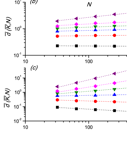
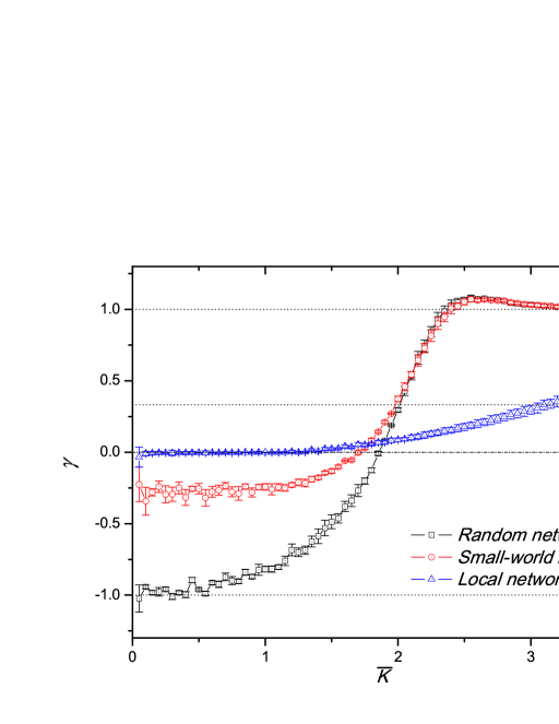
Figure 1 shows the power-law dependence of the Hamming distance $\bar{d}$ as a function of the system size $N$ for multiple $\bar{K}$ and for our three types of random network classes. $\gamma_{R}$ as a function of the average degree $\bar{K}$ is shown in Fig. 2.

Figure 1: The Hamming distance $\bar{d}$ as a function of the system size $N$ for (a) random networks, (b) networks with spatially local connections, and (c) small-world networks, for different $\bar{K}$. $\bar{K}$ takes the values $2.6$, $2.2$, $2.0$, $1.8$, $1.5$, and $1.0$, from top to bottom. The data for the random networks confirms the data as first presented in ROHLF_PRL2007 . Averaged over $10,000$ randomly generated networks and $100$ random initial configurations for each value of $\bar{K}$. $T=1000$ system updates, initial damage size $d(0)=1$.

Figure 2: Scaling exponents $\gamma(\bar{K})$ as a function of $\bar{K}$ for random networks (open squares), networks with local connections (open triangles), and small-world networks (open circles). This figure is obtained from the best fit of the data of Fig. 1 using Eq. (6), (7), and (10). The data for the random networks confirms the data as first presented in ROHLF_PRL2007 .

II.2 RBNs with Spatially Local Connections

Many real-world networks are spatially extended and have a more structured interconnect topology than pure random networks have. Such networks are commonly called complex networks. Spatial networks with local connections only, such as regular grids, have a large average path length ($l\sim N^{1/d}$) and are highly clustered. In this section, we look at the dynamics of spatial RBNs with local connections only. The underlying network structure is constructed based on the model of Uniform Spatial Graphs Watts03 , in which vertices may connect uniformly at random to other vertices within a spatial distance $l_{c}$ in $\mathbb{R}^{d}$. We do this as following: $N$ nodes are randomly distributed in a $d$-dimensional space (only $d=2$ will be considered here), we then randomly pick a pair of nodes $u$,$v$ and create edge $(u,v)$ if the spatial distance is within the cut-off distance $l_{c}$, disallowing repeated edges. This procedure is repeated until the required average degree $\bar{K}$ is reached.

For a small cutoff distance, or any finite cutoff when $N\rightarrow\infty$, e.g., $l_{c}\sim O(1)$, the characteristic path length remains similar to that of $d$-dimensional regular lattices Watts03 . For very large $\bar{K}$, the system is in the chaotic regime and any initial damage quickly percolates through the network. Thus, the damage is only bounded by the system size $N$, which gives us $\bar{d}_{L}\sim N^{1}$. In the limit of $\bar{K}\rightarrow 0$, nonzero damage can emerge only when the initial perturbation hits a short loop of oscillating nodes. Let us assume we have a single connection from node $A$ to node $B$ ($A\rightarrow B$). In order to finish a simple loop between $A$ and $B$, we need to first select node $B$ as the starting point, which has a probability of about $\sim 1/N$. The probability to pick $A$ as a neighboring node from $B$ to close the loop is $\sim 1/n_{B}$, where $n_{B}$ is the possible number of $B$’s local neighbors. For a purely local network, $n_{B}\ll N$. In a network of extreme local connections, the probability of forming simple oscillating loops scales with $P_{loop}\sim 1/n_{B}N\sim N^{-1}$. The number of such loops scales with $\sim P_{loop}\bar{K}N\sim const.$, and is thus independent of the system size $N$. We expect to see coinciding Hamming distances at low $\bar{K}$ for different system sizes $N$ on extremely local networks. This remains valid until the network reaches the percolation threshold where segregated simple loops become connected and a giant cluster emerges. Furthermore, compared to random networks, the local connections lowered the probability of forming the relevant component at criticality because each relevant node needs to be controlled by another relevant node. We thus expect that the damage increases slower compared to random networks. In particular, the exponent is smaller than $1/3$ at $K_{c}$ because $\gamma=1/3$ at $K_{c}$ for random networks ROHLF_PRL2007 .

Fig. 1(a) shows the Hamming distance as a function of the system size $N$ for different connectivities $\bar{K}$. As one can see, for small $\bar{K}$, the damage remains constant as $N$ increases. While for large $\bar{K}$ (above the percolation limit) the damage spreading increases with the system size $N$ according to a power-law. We therefore have:

$$\bar{d}_{L}(\bar{K},N)\sim a(\bar{K})N^{\gamma_{L}(\bar{K})}\;,$$ (7)

where $\gamma_{L}\rightarrow 0$ at $\bar{K}\rightarrow 0$, and $\gamma_{L}\rightarrow 1$ for large $\bar{K}$. If we do a best fit for the data as shown in Fig. 1(a) using Eq. (6), (7), we obtain $\gamma_{L}$ as a function of $\bar{K}$. This is shown in Fig. 2.

Finally, Fig. 3(d) shows the average Hamming distance for an initial damage size of one for local networks with different system sizes $N$. As one can see, all curves coincide below the percolation threshold. This confirms again our assumption of the scaling behavior for low $\bar{K}$.

II.3 RBNs with a Small-World Topology

Figure 3: Average Hamming distance (damage) $\bar{d}$ after $200$ system updates, averaged over $10,000$ randomly generated networks and $100$ random initial configurations for each value of $\bar{K}$. The initial damage size is one. Network topologies: (a) random networks ($p=1.0$, $q=0$), (b) small-world network with $p=0.9$ ($q=0.1$), (c) small-world networks with $p=0.8$ ($q=0.2$), and (d) networks with completely local connections ($p=0$, $q=1.0$). (a), (b), and (c) suggest that all curves of random and small-world networks for different $N$ approximately intersect in a characteristic point $K_{s}$. $K_{s}$ moves toward small $\bar{K}$ as the fraction of local connections increases ($K_{s}\simeq 1.875$ in (a), $K_{s}\simeq 1.80$ in (b) and $K_{s}\simeq 1.75$ in (c)). For complete local networks all curves coincide below the percolation threshold independently of $N$.

Both purely random and purely local networks are extreme network topologies. Many biological, technological, and social networks lie somewhere between these two extremes and are categorized as “small-world networks” WATTS98 . Small-world networks typically exhibit a number of advantages over locally connected networks, such as a short average path length, synchronizability, and improved robustness against certain types of failures. It is therefore of fundamental interest to study the damage spreading in RBN networks with a small-world interconnect topology.

Starting from the $2D$ Uniform Spatial Graph we have used above for the locally interconnected network, we apply a simply rewiring strategy to construct a small-world network. Each existing connection in the Uniform Spatial Graph is rewired with probability $p$ to a randomly chosen node. Thus, a fraction of $p$ links in the network are random long-range links, or small-world links, while the remaining fraction of $q=1-p$ links are local links connecting geometrically local neighbors. We will use $q$ as the main parameter to represent the “strength” of the local connections. Combined with the system size $N$, $Nq$ is approximately the number of nodes that have a local connection (at the sparse percolation limit). For $Nq\ll 1$ the network is in the random network regime (see Sec II.1); and for $Nq\gg 1$ we obtain a spatially local network (see Sec II.2).

We will now use a similar scaling approach for small-world RBNs as presented above for local and random networks. Again, at very large $\bar{K}$, the damage will only be bounded by the system size, thus $\bar{d}_{SW}\sim N^{1}$. But for $\bar{K}\rightarrow 0$, the network is now composed of both local and random (longer range) connections and the probability of forming simple loops scales thus differently. Let us assume we have a local link that has already been connected ($A\rightarrow B$). The probability of having such a local link is $q$, and to complete a simple loop that contains this local connection, we first need to pick node $B$ with probability $1/N$. Node $B$ will then establish connections again with his local neighbors with probability $q$, and finally choose node $A$ to finish the loop with probability $1/n_{B}$. Thus, the final probability of having a simple loop in this case scales with $P_{loopL}\sim q^{2}/N$. Similarly the probability of generating a simple loop involving random long-range links is $P_{loopR}\sim p^{2}/N^{2}$. We compare these two probabilities by dividing one by another:

$$\frac{P_{loopL}}{P_{loopR}}=\frac{q^{2}}{N}/\frac{p^{2}}{N^{2}}=(Nq)\cdot\frac{q}{p^{2}}\;.$$ (8)

In the spatially local network limit ($Nq\gg 1$), $P_{loopL}$ is the leading term and the scaling follows Eq. (7). In the random network limit ($Nq\ll 1$), $P_{loopR}$ dominates and the scaling follows Eq. (6). However, when the network is in the small-world regime, $P_{loopL}$ and $P_{loopR}$ become comparable. With some corrections, we therefore have:

$$P_{loopSW}=P_{loopL}+P_{loopR}=\frac{q^{2}}{N}+\frac{p^{2}}{N^{2}}\simeq\frac{1}{N^{\beta}}\;,$$ (9)

where $\beta$ is somewhere between $1$ and $2$ and depends on the value of $Nq$. The damage spreading scales therefore with $\bar{d}_{SW}\sim N^{1-\beta}$. And for general $\bar{K}$, we obtain:

$$\bar{d}_{SW}(\bar{K},N)\sim a(\bar{K})N^{\gamma_{SW}(\bar{K})}\;,$$ (10)

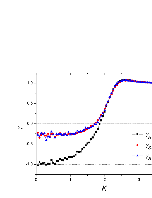
where $\gamma_{SW}$ is somewhere between $1-\beta$ to $1$. Fig. 2 shows $\gamma_{R}$, $\gamma_{L}$, and $\gamma_{SW}$. As one can see, $\gamma_{SW}$ goes from $1-\beta$, which is below zero, to $1$ as $\bar{K}$ increases. In addition, the critical connectivity $\bar{K}$, where $\gamma_{SW}=0$, is different from random networks and depends $q$. In random networks this point is defined as the critical degree of stability $K_{s}$ ROHLF_PRL2007 . Our results show that the introduction of local connections in random networks changes $K_{s}$ toward lower $\bar{K}$. As we have seen above, in extreme local networks $K_{s}$ is undefined because the Hamming distance for different system sizes $N$ simply coincide below the percolation threshold. Fig. 3 (c) shows the deviation of $K_{s}$ from the observed value $K_{s}=1.875$ for random networks.

II.4 Finite-size Scaling in Random Small-World RBNs

Figure 4: Hamming distance $\bar{d}$ for different average degrees $\bar{K}$ as a function of the density of local connections $q$. The inset shows $\bar{d}$ in the range of random networks ($q\rightarrow 0$) to local networks ($q\rightarrow 1$). The different curves range from (top to bottom) $\bar{K}=2.2$ to $\bar{K}=1.02$ with an interval of $0.2$.

Figure 5: Reconstructed $\gamma_{SW}$ from Eq. 15 by measuring $\alpha(\bar{K})$ from best fits of Fig. 4 at $q=0.2$ ($p=0.8$). Squares (black) and circles (red) are measured $\gamma_{R}$ and $\gamma_{SW}$, respectively, from Fig. 1, while triangles (blue) are reconstructed $\gamma_{SW}$ from $\gamma_{R}$ and $\alpha(\bar{K})$.

Figure 6: Scaling plots of the Hamming distance in small-world networks as predicted by the finite-size scaling argument (Eq. (16)). (a) $\bar{K}=1.4$; (b) $\bar{K}=2.0$; and (c) $\bar{K}=3.0$. The straight line segments correspond to asymptotic power-law behavior of the scaling function $g(x)$ with exponents $\gamma_{R}$ and $\gamma_{L}$, measured from Fig. 2 at given $\bar{K}$, for small and large arguments, respectively, as described in the text (Eq. (17)).

While Eqs. (6) and (7) provide the scaling of the Hamming distance for random and local networks, we are interested in this section how $q$ (i.e., the fraction of local links) affects the damage spreading.

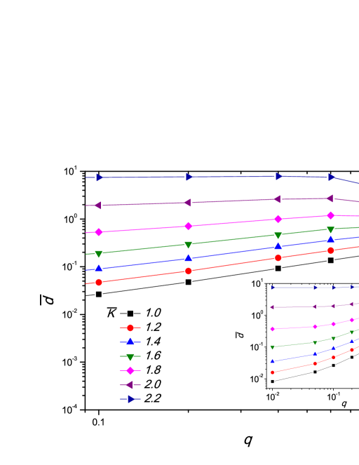
Fig. 4 shows the hamming distance as a function of $q$. For sufficiently large $Nq$, i.e., close to the local network limit, we assume (see Fig. 4) that the Hamming distance approaches an asymptotic power law $\bar{d}_{SW}\sim q^{\alpha(\bar{K})}$. On the other hand, the Hamming distance also depends on the system size with $\bar{d}_{SW}\sim N^{\gamma_{SW}(\bar{K})}$ (see Eq. (10)). Thus, in the small-world regime (close to the local network limit) the Hamming distance depends on both the system size and the density of local (random) connections:

$$\bar{d}_{SW}(q,\bar{K},N)\sim q^{\alpha(\bar{K})}N^{\gamma_{SW}(\bar{K})}\;.$$ (11)

When $q\rightarrow 1$, $\gamma_{SW}(\bar{K})\rightarrow\gamma_{L}(\bar{K})$, so $\bar{d}_{SW}\rightarrow\bar{d}_{L}$. While in the random network limit ($Nq\ll 1$), $\bar{d}$ only depends on $N$, $\bar{d}_{R}\sim N^{\gamma_{R}(\bar{K})}$ with $\gamma_{R}(\bar{K})$ as illustrated in Fig. 2. To connect the above two cases and to capture the finite-size behavior in the small-world regime, one can construct the full scaling behavior of $\bar{d}_{SW}(q,\bar{K},N)$:

$$\bar{d}_{SW}(q,\bar{K},N)\sim q^{\alpha(\bar{K})}N^{\gamma_{SW}(\bar{K})}f(Nq)\;,$$ (12)

where $f(x)$ is a scaling function such that

$$f(x)\sim\left\{\begin{array}[]{ll}x^{-\alpha}&\mbox{if $x$$\ll$$1$}\\ {\rm const.}&\mbox{if $x$$\gg$$1$}\end{array}\right.\;.$$ (13)

The random network limit is obtained provided that

$$\bar{d}\sim q^{\alpha(\bar{K})}N^{\gamma_{SW}(\bar{K})}(Nq)^{-\alpha}\sim N^{\gamma_{SW}-\alpha}\sim N^{\gamma_{R}}\;,$$ (14)

i.e.,

$$\gamma_{R}=\gamma_{SW}-\alpha(\bar{K})\;.$$ (15)

Given $\gamma_{R}$ we can express $\gamma_{SW}$ by measuring $\alpha(\bar{K})$ at different $\bar{K}$. Fig. 5 shows the reconstructed $\gamma_{SW}$ with the measured data, which satisfy the above proposed asymptotic scaling relation.

To analyze our data, Eq. (12) can also be written as

$$\bar{d}_{SW}(q,\bar{K},N)\sim\frac{(Nq)^{\gamma_{SW}}}{q^{\gamma_{SW}-\alpha}}f(Nq)\sim\frac{1}{q^{\gamma_{R}}}g(Nq)\;,$$ (16)

where $g(x)=x^{\gamma_{SW}}f(x)$. Thus plotting $\bar{d}q^{\gamma_{R}}$ vs. $Nq$ should yield coinciding data with $g(x)$. The limits of random and spatially local networks correspond to the asymptotic small and large argument of $g(x)$, which gives us the exponents $\gamma_{R}$, and $\gamma_{L}$,

$$g(x)\sim\left\{\begin{array}[]{ll}x^{\gamma_{\rm R}}&\mbox{if $x$$\ll$$1$}\\ x^{\gamma_{\rm SW}}\rightarrow x^{\gamma_{\rm L}}&\mbox{if $x$$\gg$$1$}\end{array}\right.\;.$$ (17)

Fig. 6 shows the scaling plots of the Hamming distance as a function of the product of the system size $N$ and strength of the local connections $q$, as predicted by the proposed finite-size scaling for small-world RBNs. Also, given that $\gamma_{R}$ and $\gamma_{L}$ are functions of the average degree $\bar{K}$, as shown in Fig. 2, the shapes of $f(x)$ or $g(x)$ also changes with $\bar{K}$. As one can see in Fig. 6(a)-(c), $g(x)$ coincides under different $\bar{K}$. In addition, the asymptotic behavior of $g(x)$ at $x\ll 1$ and $x\gg 1$ agree very well with our measured “phenomenological” exponents $\gamma_{R}(\bar{K})$, and $\gamma_{L}(\bar{K})$ at $\bar{K}=1.4$, $\bar{K}=2.0$, and $\bar{K}=4.0$, respectively.

III Wiring Cost

Figure 7: The product of damage size $d$, the network wiring cost $cost$, and the average shortest path length $l$ as a function of the average connectivity $\bar{K}$ and the density of random connections $p$. The color density corresponds to the value of $d\times l\times cost$

Figure 8: Contour projection of Fig. 7. The color density corresponds to the value of $d\times l\times cost$. At $p=0$ the network topology is completely local; $p=1$ corresponds to the random network; and for $0<p<1$ the network is in the small-world regime. The circles indicate the position of lowest possible $\bar{K}$ and corresponding $p$ for given tolerance level of $d\times l\times cost$.

From an engineering perspective, one wants to typically minimize the wiring cost of a network, maximize the communication characteristics, and maximize the robustness against failures. The electric power grid is a good example and so are nano-scale interconnect networks teuscher07:chaos . In this section we will look at these three trade-offs for RBNs.

The average shortest path length is generally a good measure for the communication characteristics of a complex network. In a directed network we define $l$ as the mean geodesic (i.e., shortest) distance between vertex pairs in a network Newman_2003 :

$$l=\frac{1}{n(n-1)}\sum_{i\neq j}d_{ij}\;,$$ (18)

where $d_{ij}$ is the geodesic distance from vertex $i$ to vertex $j$. Here we have excluded the distance from each node to itself. Eq. 18 will be problematic if the network has more than one component, which is very likely for small $\bar{K}$. To avoid the problem of disconnected networks, we compute the average path length only for those vertex pairs that actually have a connecting path between them.

For real-world networks, if shortcuts, i.e., the random small-world links, have to be realized physically, the cost of a long-range connection is likely to grow with its length. E.g., the power consumption for wireless broadcast communication in free space generally could be a cubic power of geometric distance, while the implementation of directional antenna will reduce the transmission cost significantly Huang06 . Petermann et al. Petermann05 discuss the wiring-cost for some spatial small-world networks ranging from integrated circuits, the Internet to cortical networks. For simplicity, we assume here that the wiring cost has a linear dependency on the geometrical distance between two nodes.

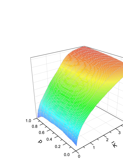
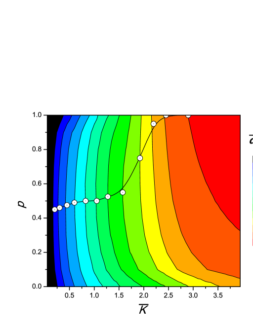
Fig. 7 shows the product of the wiring cost $cost$, the average shortest path length $l$, and the damage size $\bar{d}$ as a function of the average connectivity $\bar{K}$ and the density of random connections $p$. In addition, Fig. 8 shows the contour projection of Fig. 7 using the same data. For example, it shows that given a specific target average connectivity $\bar{K}$, networks with a high density of random connections (i.e., close to random networks, $p\to 1$) will have a similar overall performance, cost, and robustness as networks that have more local connections ($p\to 0$), however, whereas $p\to 1$ networks have a high wiring cost, a low average path length, and a low damage resistivity, $p\to 0$ networks have a low wiring cost, a high average path length, and a high damage resistivity. Fig. 8 also tells us what will be the lowest $\bar{K}$ and corresponding $p$ allowed at a given robustness level. This is indicated by the circles.

IV Conclusion

We have systematically investigated the damage spreading in spatial and small-world random Boolean networks. We have found that (1) spatially local connections change the scaling of the relevant component at very low connectivities ($\bar{K}\ll 1$) and (2) that the critical connectivity of stability $K_{s}$ changes compared to random networks ROHLF_PRL2007 . At higher $\bar{K}$, this scaling remains unchanged. We also show that the relevant component of spatially local networks scales with a power-law as the system size N increases, but with a different exponent for local and small-world networks. The scaling behaviors are obtained by finite-size scaling. In addition, we have investigated the trade-offs between the wiring cost of the networks, the communication characteristics, and the robustness, i.e., the damage spreading. From an engineering perspective, one typically wants to minimize the wiring cost, maximize the communication characteristics, e.g., the shortest path between any two nodes, and maximize the robustness against failures. Our new findings provide these key trade-offs and allow to determine the lowest connectivity $\bar{K}$ and the amount of randomness $p$ in a network for a given robustness, average path length, and wiring cost.

Future work will focus on the investigation of real-world networks and the application of our methodology to make them more robust, cheaper, and more efficient.