The Clausius inequality beyond the weak coupling limit:
The quantum Brownian oscillator revisited

Ilki Kim1 hannibal.ikim@gmail.com    Günter Mahler2 1Department of Physics, North Carolina A&\&T State University, Greensboro, NC 27411
2Institute of Theoretical Physics I, University of Stuttgart, 70550 Stuttgart, Germany
Abstract

We consider a quantum linear oscillator coupled at an arbitrary strength to a bath at an arbitrary temperature. We find an exact closed expression for the oscillator density operator. This state is non-canonical but can be shown to be equivalent to that of an uncoupled linear oscillator at an effective temperature Teffsuperscriptsubscript𝑇effT_{\text{\scriptsize eff}}^{\star} with an effective mass and an effective spring constant. We derive an effective Clausius inequality δ𝒬effTeffdS𝛿superscriptsubscript𝒬effsuperscriptsubscript𝑇eff𝑑𝑆\delta{\mathcal{Q}}_{\text{\scriptsize eff}}^{\star}\leq T_{\text{\scriptsize eff}}^{\star}\,dS, where δ𝒬eff𝛿superscriptsubscript𝒬eff\delta{\mathcal{Q}}_{\text{\scriptsize eff}}^{\star} is the heat exchanged between the effective (weakly coupled) oscillator and the bath, and S𝑆S represents a thermal entropy of the effective oscillator, being identical to the von-Neumann entropy of the coupled oscillator. Using this inequality (for a cyclic process in terms of a variation of the coupling strength) we confirm the validity of the second law. For a fixed coupling strength this inequality can also be tested for a process in terms of a variation of either the oscillator mass or its spring constant. Then it is never violated. The properly defined Clausius inequality is thus more robust than assumed previously.

pacs:
05.40.-a, 05.70.-a

I Introduction

Thermodynamics of small quantum objects coupled to quantum environments in the low temperature regime has attracted considerable interest as the need for a better theoretical understanding increases in response to novel experimental manipulation of such systems. In particular, the finite coupling strength between system and environment gives rise to some quantum subtleties and so can no longer be neglected (calling for methods addressed by ‘quantum thermodynamics’ SHE02 ; MAH04 ; CAP05 ) whereas ordinary quantum statistical mechanics is intrinsically based on a vanishingly small coupling between them.

At the heart of quantum thermodynamics, the foundational question as to the validity of the second law of thermodynamics comes up. In fact, with its challenge the applicability of thermodynamics is at stake. So far, the validity of this basic law has extensively been examined in the scheme of a quantum harmonic oscillator linearly coupled to an independent-oscillator model of a heat bath (quantum Brownian oscillator) in equilibrium at a low temperature T𝑇T. It has been argued here that there is a violation of the Clausius inequality representing the second law ALL00 ; NIE02 in such a way that δ𝒬TdSnot-less-than-or-equals𝛿𝒬𝑇𝑑𝑆\delta{\mathcal{Q}}\not\leq T\,dS at T0𝑇0T\to 0 with respect to a variation of a Hamiltonian parameter of the coupled oscillator, namely, either its mass or spring constant. In the above relation, δ𝒬𝛿𝒬\delta{\mathcal{Q}} is the heat and dS𝑑𝑆dS is the entropy change.

However, following the second law in its Kelvin-Planck form, which states that it is impossible to devise a machine (i.e., a heat engine) which, operating in a cycle, produces no effect other than the extraction of heat from a thermal energy reservoir and the performance of an equal amount of work ANN02 , it has been demonstrated that an apparent excess energy in the coupled oscillator at zero temperature (T=0)𝑇0(T=0) is less than the minimum value of the work (equivalent to the Helmholtz free energy at a constant temperature) to couple the free oscillator to a bath so that the second law is not violated down to zero temperature FOR06 ; KIM06 .

This result has been generalized to a cyclic process of coupling and decoupling between the oscillator and a bath at an arbitrary temperature by obtaining the positive-valuedness of the minimum work needed for the coupling minus the maximum useful work obtainable from the oscillator in the decoupling (the second law with respect to a variation of the coupling strength) KIM07 . This positive-valuedness is actually at its maximum at zero temperature and asymptotically vanishes with increasing temperature, whereas the classical counterpart would identically vanish at an arbitrary temperature (even for a non-vanishing coupling). It was further claimed here that this quantum behavior is associated with the system-bath entanglement induced by the finite coupling strength between them (clearly, the coupled total system (i.e., the coupled oscillator plus bath) is in a thermal state with (partial) entanglement whereas the decoupled total system is simply in a separable state). It has, indeed, been found that at zero temperature the energy fluctuation in the coupled oscillator can provide entanglement information BUE04 ; BUE05 . This claim was supported by the numerical analysis of the system-bath negativity as an exact entanglement measure LUT08 that the negativity behavior versus temperature is in accordance with the above quantum behavior of the second law up to the existence of the critical temperature above which the negativity vanishes.

It has also been shown LUT08 that the Clausius inequality (in terms of the equilibrium temperature of the total coupled system and the von-Neumann entropy of the coupled oscillator) is actually violated with respect to a variation of the mass of the coupled oscillator (not a variation of the coupling strength); the behavior of this violation versus the temperature is essentially different from that of the system-bath negativity so that it has been concluded that the system-bath entanglement is not responsible for the violation of the Clausius inequality. However, as the reduced equilibrium density operator of the coupled oscillator is not in form of the canonical thermal state ρ^βeβH^sproportional-tosubscript^𝜌𝛽superscript𝑒𝛽subscript^𝐻𝑠\hat{\rho}_{\beta}\propto e^{-\beta\hat{H}_{s}}, there is not a well-defined local temperature of the coupled oscillator (especially in the low temperature limit) so that applying the equilibrium temperature of the total coupled system for the violation of the Clausius inequality for the subsystem (actually with respect to a variation of a local parameter of the coupled oscillator, namely, either its mass or spring constant) is not justified. Further, this violation was actually based on the numerical findings LUT08 that the heat δ𝒬𝛿𝒬\delta{\mathcal{Q}} exchanged with a bath in a reversible variation of the local parameter is always strictly greater than TdS𝑇𝑑𝑆T\,dS, which, however, does not satisfy the equality condition of a well-defined Clausius inequality for the reversible process.

On the other hand, introducing some generalized entropic measure and using its maximum condition THU07 it has been shown that the Clausius inequality obtained in some operational form is valid under such a generalization ABE08 . However, this approach is not directly applicable for the quantum Brownian oscillator since the reduced density operator of the coupled oscillator in equilibrium (cf. equations (17) and (18)) is not in form of the stationary state obtained from the maximum condition of this generalization.

In this paper we intend to resolve the above controversial issue by introducing an effective Clausius inequality with no violation, well-defined in the scheme of quantum Brownian oscillator. To do so, we begin with considering the reduced density operator of the coupled oscillator.

II Reduced density operator of the coupled oscillator

The quantum Brownian motion in consideration is described by the model Hamiltonian

H^=H^s+H^b+H^sb,^𝐻subscript^𝐻𝑠subscript^𝐻𝑏subscript^𝐻𝑠𝑏\hat{H}\;=\;\hat{H}_{s}\,+\,\hat{H}_{b}\,+\,\hat{H}_{sb}\,, (1)

where

H^s=p^22M+k02q^2;H^b=j=1N(p^j22mj+kj2x^j2)formulae-sequencesubscript^𝐻𝑠superscript^𝑝22𝑀subscript𝑘02superscript^𝑞2subscript^𝐻𝑏superscriptsubscript𝑗1𝑁superscriptsubscript^𝑝𝑗22subscript𝑚𝑗subscript𝑘𝑗2superscriptsubscript^𝑥𝑗2\displaystyle\displaystyle\hat{H}_{s}\,=\,\frac{\hat{p}^{2}}{2M}+\frac{k_{0}}{2}\,\hat{q}^{2}\;\;\;;\;\;\;\hat{H}_{b}\,=\,\sum_{j=1}^{N}\left(\frac{\hat{p}_{j}^{2}}{2m_{j}}+\frac{k_{j}}{2}\,\hat{x}_{j}^{2}\right)
H^sb=q^j=1Ncjx^j+q^2j=1Ncj22kj,subscript^𝐻𝑠𝑏^𝑞superscriptsubscript𝑗1𝑁subscript𝑐𝑗subscript^𝑥𝑗superscript^𝑞2superscriptsubscript𝑗1𝑁superscriptsubscript𝑐𝑗22subscript𝑘𝑗\displaystyle\displaystyle\hat{H}_{sb}\,=\,-\hat{q}\sum_{j=1}^{N}c_{j}\,\hat{x}_{j}\,+\,\hat{q}^{2}\sum_{j=1}^{N}\frac{c_{j}^{2}}{2\,k_{j}}\,, (2)

and the spring constants are k0=Mω02subscript𝑘0𝑀superscriptsubscript𝜔02k_{0}=M\omega_{0}^{2} and kj=mjωj2subscript𝑘𝑗subscript𝑚𝑗superscriptsubscript𝜔𝑗2k_{j}=m_{j}\,\omega_{j}^{2}. From the hermiticity of Hamiltonian, the coupling constants cjsubscript𝑐𝑗c_{j} are obviously real-valued. The total system is assumed to be in the canonical thermal equilibrium state ρ^β=eβH^/Zβsubscript^𝜌𝛽superscript𝑒𝛽^𝐻subscript𝑍𝛽\hat{\rho}_{\beta}=e^{-\beta\hat{H}}/Z_{\beta} where β=1/(kBT)𝛽1subscript𝑘𝐵𝑇\beta=1/(k_{B}\,T), and Zβsubscript𝑍𝛽Z_{\beta} is the partition function. From the fluctuation-dissipation theorem CAL51 ; WEI99 , it is known FOR85 that

q^2βsubscriptdelimited-⟨⟩superscript^𝑞2𝛽\displaystyle\textstyle\langle\hat{q}^{2}\rangle_{\beta} =\displaystyle= π0𝑑ωcoth(βω2)Im{χ~(ω+i 0+)}Planck-constant-over-2-pi𝜋superscriptsubscript0differential-d𝜔hyperbolic-cotangent𝛽Planck-constant-over-2-pi𝜔2Im~𝜒𝜔𝑖superscript 0\displaystyle\textstyle\frac{\hbar}{\pi}\,\int_{0}^{\infty}d\omega\,\coth\left(\frac{\beta\hbar\omega}{2}\right)\,\text{Im}\{\tilde{\chi}(\omega+i\,0^{+})\} (3)
p^2βsubscriptdelimited-⟨⟩superscript^𝑝2𝛽\displaystyle\textstyle\langle\hat{p}^{2}\rangle_{\beta} =\displaystyle= M2π0𝑑ωω2coth(βω2)Im{χ~(ω+i 0+)}superscript𝑀2Planck-constant-over-2-pi𝜋superscriptsubscript0differential-d𝜔superscript𝜔2hyperbolic-cotangent𝛽Planck-constant-over-2-pi𝜔2Im~𝜒𝜔𝑖superscript 0\displaystyle\textstyle\frac{M^{2}\hbar}{\pi}\,\int_{0}^{\infty}d\omega\,\omega^{2}\,\coth\left(\frac{\beta\hbar\omega}{2}\right)\,\text{Im}\{\tilde{\chi}(\omega+i\,0^{+})\} (4)

in terms of the susceptibility

χ~(ω)=1Mj=1N(ω2ωj2)k=0N(ω2ω¯k2)~𝜒𝜔1𝑀superscriptsubscriptproduct𝑗1𝑁superscript𝜔2superscriptsubscript𝜔𝑗2superscriptsubscriptproduct𝑘0𝑁superscript𝜔2superscriptsubscript¯𝜔𝑘2\tilde{\chi}(\omega)\;=\;-\frac{1}{M}\,\frac{\displaystyle\prod_{j=1}^{N}\,(\omega^{2}-\omega_{j}^{2})}{\displaystyle\prod_{k=0}^{N}\,(\omega^{2}-\bar{\omega}_{k}^{2})} (5)

where {ω¯k}subscript¯𝜔𝑘\{\bar{\omega}_{k}\} are the normal-mode frequencies of the total system H^^𝐻\hat{H}. For an uncoupled oscillator, Imχ~(ω+i0+)Im~𝜒𝜔𝑖superscript0\text{Im}\,\tilde{\chi}(\omega+i0^{+}) obviously reduces to π2Mω0δ(ωω0)𝜋2𝑀subscript𝜔0𝛿𝜔subscript𝜔0\frac{\pi}{2M\omega_{0}}\delta(\omega-\omega_{0}) and thus q^2β=2Mω0cothβω02subscriptdelimited-⟨⟩superscript^𝑞2𝛽Planck-constant-over-2-pi2𝑀subscript𝜔0hyperbolic-cotangent𝛽Planck-constant-over-2-pisubscript𝜔02\langle\hat{q}^{2}\rangle_{\beta}=\frac{\hbar}{2M\omega_{0}}\coth\frac{\beta\hbar\omega_{0}}{2} and p2β=Mω02cothβω02subscriptdelimited-⟨⟩superscript𝑝2𝛽𝑀Planck-constant-over-2-pisubscript𝜔02hyperbolic-cotangent𝛽Planck-constant-over-2-pisubscript𝜔02\langle p^{2}\rangle_{\beta}=\frac{M\hbar\omega_{0}}{2}\coth\frac{\beta\hbar\omega_{0}}{2}. For the well-known Drude model (with a cut-off frequency ωdsubscript𝜔𝑑\omega_{d} and a damping parameter γosubscript𝛾𝑜\gamma_{o}), which is a prototype for physically realistic damping, we have KIM07

q^2β(d)superscriptsubscriptdelimited-⟨⟩superscript^𝑞2𝛽𝑑\displaystyle\langle\hat{q}^{2}\rangle_{\beta}^{(d)} =\displaystyle= 1Ml=13λd(l){1βωl¯+πψ(βωl¯2π)}1𝑀superscriptsubscript𝑙13superscriptsubscript𝜆𝑑𝑙1𝛽¯subscript𝜔𝑙Planck-constant-over-2-pi𝜋𝜓𝛽Planck-constant-over-2-pi¯subscript𝜔𝑙2𝜋\displaystyle{\textstyle\frac{1}{M}}\sum_{l=1}^{3}{\textstyle\lambda_{d}^{(l)}\,\left\{\frac{1}{\beta\underline{\omega_{l}}}\,+\,\frac{\hbar}{\pi}\;\psi\left(\frac{\beta\hbar\underline{\omega_{l}}}{2\pi}\right)\right\}} (6)
p^2β(d)superscriptsubscriptdelimited-⟨⟩superscript^𝑝2𝛽𝑑\displaystyle\langle\hat{p}^{2}\rangle_{\beta}^{(d)} =\displaystyle= Ml=13λd(l)ωl¯2{1βωl¯+πψ(βωl¯2π)}𝑀superscriptsubscript𝑙13superscriptsubscript𝜆𝑑𝑙superscript¯subscript𝜔𝑙21𝛽¯subscript𝜔𝑙Planck-constant-over-2-pi𝜋𝜓𝛽Planck-constant-over-2-pi¯subscript𝜔𝑙2𝜋\displaystyle{\textstyle-M}\sum_{l=1}^{3}{\textstyle\lambda_{d}^{(l)}\,\underline{\omega_{l}}^{2}\,\left\{\frac{1}{\beta\underline{\omega_{l}}}\,+\,\frac{\hbar}{\pi}\;\psi\left(\frac{\beta\hbar\underline{\omega_{l}}}{2\pi}\right)\right\}} (7)

in terms of the digamma function ψ(y)=dlnΓ(y)/dy𝜓𝑦𝑑Γ𝑦𝑑𝑦\psi(y)=d\,\ln\Gamma(y)/dy ABS74 , where ω1¯=Ω¯subscript𝜔1Ω\underline{\omega_{1}}=\Omega, ω2¯=z1¯subscript𝜔2subscript𝑧1\underline{\omega_{2}}=z_{1}, ω3¯=z2¯subscript𝜔3subscript𝑧2\underline{\omega_{3}}=z_{2}, and the coefficients

λd(1)=z1+z2(Ωz1)(z2Ω);λd(2)=Ω+z2(z1Ω)(z2z1);λd(3)=Ω+z1(z2Ω)(z1z2).formulae-sequencesuperscriptsubscript𝜆𝑑1subscript𝑧1subscript𝑧2Ωsubscript𝑧1subscript𝑧2Ωformulae-sequencesuperscriptsubscript𝜆𝑑2Ωsubscript𝑧2subscript𝑧1Ωsubscript𝑧2subscript𝑧1superscriptsubscript𝜆𝑑3Ωsubscript𝑧1subscript𝑧2Ωsubscript𝑧1subscript𝑧2\textstyle\lambda_{d}^{(1)}\;=\;\frac{z_{1}\,+\,z_{2}}{(\Omega\,-\,z_{1})(z_{2}\,-\,\Omega)}\;;\;\lambda_{d}^{(2)}\;=\;\frac{\Omega\,+\,z_{2}}{(z_{1}\,-\,\Omega)(z_{2}\,-\,z_{1})}\;;\;\lambda_{d}^{(3)}\;=\;\frac{\Omega\,+\,z_{1}}{(z_{2}\,-\,\Omega)(z_{1}\,-\,z_{2})}\,. (8)

Here we have adopted, in place of (ω0,ωd,γo)subscript𝜔0subscript𝜔𝑑subscript𝛾𝑜(\omega_{0},\omega_{d},\gamma_{o}), the parameters (𝐰0,Ω,γ)subscript𝐰0Ω𝛾({\mathbf{w}}_{0},\Omega,\gamma) through the relations FOR06

ω02:=𝐰02ΩΩ+γ;ωd:=Ω+γ;γo:=γΩ(Ω+γ)+𝐰02(Ω+γ)2,formulae-sequenceassignsuperscriptsubscript𝜔02superscriptsubscript𝐰02ΩΩ𝛾formulae-sequenceassignsubscript𝜔𝑑Ω𝛾assignsubscript𝛾𝑜𝛾ΩΩ𝛾superscriptsubscript𝐰02superscriptΩ𝛾2\textstyle\omega_{0}^{2}\,:=\,{\mathbf{w}}_{0}^{2}\;\frac{\Omega}{\Omega\,+\,\gamma}\;\;;\;\;\omega_{d}\,:=\,\Omega\,+\,\gamma\;\;;\;\;\gamma_{o}\,:=\,\gamma\,\frac{\Omega\,(\Omega\,+\,\gamma)\,+\,{\mathbf{w}}_{0}^{2}}{(\Omega\,+\,\gamma)^{2}}\,, (9)

and then z1=γ/2+i𝐰1subscript𝑧1𝛾2𝑖subscript𝐰1z_{1}=\gamma/2+i{\mathbf{w}}_{1} and z2=γ/2i𝐰1subscript𝑧2𝛾2𝑖subscript𝐰1z_{2}=\gamma/2-i{\mathbf{w}}_{1} with 𝐰1=(𝐰0)2(γ/2)2subscript𝐰1superscriptsubscript𝐰02superscript𝛾22{\mathbf{w}}_{1}=\sqrt{({\mathbf{w}}_{0})^{2}-(\gamma/2)^{2}}.

The equilibrium density operator of the coupled oscillator is known as WEI99 ; ING88

q|ρ^s|q=12πq^2βexp((q+q)28q^2βp^2β(qq)222).quantum-operator-product𝑞subscript^𝜌𝑠superscript𝑞12𝜋subscriptdelimited-⟨⟩superscript^𝑞2𝛽superscript𝑞superscript𝑞28subscriptdelimited-⟨⟩superscript^𝑞2𝛽subscriptdelimited-⟨⟩superscript^𝑝2𝛽superscript𝑞superscript𝑞22superscriptPlanck-constant-over-2-pi2\textstyle\langle q|\hat{\rho}_{s}|q^{\prime}\rangle\,=\,\frac{1}{\sqrt{2\pi\langle\hat{q}^{2}\rangle_{\beta}}}\,\exp\left(-\frac{(q+q^{\prime})^{2}}{8\,\langle\hat{q}^{2}\rangle_{\beta}}-\frac{\langle\hat{p}^{2}\rangle_{\beta}\,(q-q^{\prime})^{2}}{2\hbar^{2}}\right)\,. (10)

For an uncoupled oscillator this easily reduces to a well-known expression FEY98

q|ρ^β|qquantum-operator-product𝑞subscript^𝜌𝛽superscript𝑞\displaystyle\textstyle\langle q|\hat{\rho}_{\beta}|q^{\prime}\rangle =\displaystyle= c2πtanhβω02exp(c24{(q+q)2tanh(βω02)+(qq)2coth(βω02)})superscript𝑐2𝜋𝛽Planck-constant-over-2-pisubscript𝜔02superscript𝑐24superscript𝑞superscript𝑞2𝛽Planck-constant-over-2-pisubscript𝜔02superscript𝑞superscript𝑞2hyperbolic-cotangent𝛽Planck-constant-over-2-pisubscript𝜔02\displaystyle\textstyle\sqrt{\frac{c^{2}}{\pi}\,\tanh\frac{\beta\hbar\omega_{0}}{2}}\,\exp\left(-\frac{c^{2}}{4}\left\{(q+q^{\prime})^{2}\tanh\left(\frac{\beta\hbar\omega_{0}}{2}\right)+(q-q^{\prime})^{2}\coth\left(\frac{\beta\hbar\omega_{0}}{2}\right)\right\}\right) (11)

where the parameter

c=Mω0.𝑐𝑀subscript𝜔0Planck-constant-over-2-pi\textstyle c\,=\,\sqrt{\frac{M\omega_{0}}{\hbar}}\,. (12)

Let us now derive a closed form of the matrix elements

ρnm:=n|ρ^s|m=𝑑q𝑑qψn(q)q|ρ^s|qψm(q)assignsubscript𝜌𝑛𝑚quantum-operator-product𝑛subscript^𝜌𝑠𝑚superscriptsubscriptsuperscriptsubscriptdifferential-d𝑞differential-dsuperscript𝑞superscriptsubscript𝜓𝑛𝑞quantum-operator-product𝑞subscript^𝜌𝑠superscript𝑞subscript𝜓𝑚superscript𝑞\textstyle\rho_{nm}\,:=\,\textstyle\langle n|\hat{\rho}_{s}|m\rangle\,=\,\textstyle\int_{-\infty}^{\infty}\int_{-\infty}^{\infty}dq\,dq^{\prime}\,\psi_{n}^{\ast}(q)\,\langle q|\hat{\rho}_{s}|q^{\prime}\rangle\,\psi_{m}(q^{\prime}) (13)

in the basis composed of the eigenstates {|n,|m}ket𝑛ket𝑚\{|n\rangle,|m\rangle\} of an uncoupled oscillator to confirm its deviation from a (diagonal) form of the canonical thermal state ρ^βsubscript^𝜌𝛽\hat{\rho}_{\beta}. After making lengthy calculations, every single step of which is provided in a detail in Appendix A, we arrive at the closed expressions

ρ2k,2l+1subscript𝜌2𝑘2𝑙1\displaystyle\rho_{2k,2{\mathit{l}}+1} =\displaystyle= ρ2k+1,2l= 0subscript𝜌2𝑘12𝑙 0\displaystyle\rho_{2k+1,2{\mathit{l}}}\,=\,0 (14a)
ρ2k,2lsubscript𝜌2𝑘2𝑙\displaystyle\rho_{2k,2{\mathit{l}}} =\displaystyle= (Υβ)k+lc2πq^2βAβΓ(k+12)k!Γ(l+12)l!F12(k,l;12;1Δβ)superscriptsubscriptΥ𝛽𝑘𝑙𝑐2𝜋subscriptdelimited-⟨⟩superscript^𝑞2𝛽subscript𝐴𝛽Γ𝑘12𝑘Γ𝑙12𝑙subscriptsubscript𝐹12𝑘𝑙121subscriptΔ𝛽\displaystyle\textstyle\frac{\left(-\Upsilon_{\beta}\right)^{k+{\mathit{l}}}}{c\;\sqrt{2\pi\,\langle\hat{q}^{2}\rangle_{\beta}\,A_{\beta}}}\,\sqrt{\frac{\Gamma\left(k+\frac{1}{2}\right)}{k!}\frac{\Gamma\left({\mathit{l}}+\frac{1}{2}\right)}{{\mathit{l}}!}}\,{}_{2}F_{1}\left(-k,-{\mathit{l}};\frac{1}{2};\frac{1}{\Delta_{\beta}}\right) (14b)
ρ2k+1,2l+1subscript𝜌2𝑘12𝑙1\displaystyle\rho_{2k+1,2{\mathit{l}}+1} =\displaystyle= 2Λβ(Υβ)k+lc2πq^2βAβΓ(k+32)k!Γ(l+32)l!F12(k,l;32;1Δβ)2subscriptΛ𝛽superscriptsubscriptΥ𝛽𝑘𝑙𝑐2𝜋subscriptdelimited-⟨⟩superscript^𝑞2𝛽subscript𝐴𝛽Γ𝑘32𝑘Γ𝑙32𝑙subscriptsubscript𝐹12𝑘𝑙321subscriptΔ𝛽\displaystyle\textstyle\frac{2\,\Lambda_{\beta}\,\left(-\Upsilon_{\beta}\right)^{k+{\mathit{l}}}}{c\;\sqrt{2\pi\,\langle\hat{q}^{2}\rangle_{\beta}\,A_{\beta}}}\,\sqrt{\frac{\Gamma\left(k+\frac{3}{2}\right)}{k!}\frac{\Gamma\left({\mathit{l}}+\frac{3}{2}\right)}{{\mathit{l}}!}}\,{}_{2}F_{1}\left(-k,-{\mathit{l}};\frac{3}{2};\frac{1}{\Delta_{\beta}}\right) (14c)

in terms of the hypergeometric function F12(a,b;c;z)subscriptsubscript𝐹12𝑎𝑏𝑐𝑧{}_{2}F_{1}(a,b;c;z) ABS74 . Here, the four dimensionless quantities

Aβ=(c2+2p^2β2)(c2+12q^2β)4c4;Υβ=p^2β2q^2βc44c4Aβ;Λβ=p^2β214q^2β2c2Aβ;Δβ=(ΥβΛβ)2.formulae-sequencesubscript𝐴𝛽superscript𝑐22subscriptdelimited-⟨⟩superscript^𝑝2𝛽superscriptPlanck-constant-over-2-pi2superscript𝑐212subscriptdelimited-⟨⟩superscript^𝑞2𝛽4superscript𝑐4formulae-sequencesubscriptΥ𝛽subscriptdelimited-⟨⟩superscript^𝑝2𝛽superscriptPlanck-constant-over-2-pi2subscriptdelimited-⟨⟩superscript^𝑞2𝛽superscript𝑐44superscript𝑐4subscript𝐴𝛽formulae-sequencesubscriptΛ𝛽subscriptdelimited-⟨⟩superscript^𝑝2𝛽superscriptPlanck-constant-over-2-pi214subscriptdelimited-⟨⟩superscript^𝑞2𝛽2superscript𝑐2subscript𝐴𝛽subscriptΔ𝛽superscriptsubscriptΥ𝛽subscriptΛ𝛽2\textstyle A_{\beta}\,=\,\frac{\left(c^{2}+\frac{2\langle\hat{p}^{2}\rangle_{\beta}}{\hbar^{2}}\right)\left(c^{2}+\frac{1}{2\langle\hat{q}^{2}\rangle_{\beta}}\right)}{4c^{4}}\;;\;\textstyle\Upsilon_{\beta}\,=\,\frac{\frac{\langle\hat{p}^{2}\rangle_{\beta}}{\hbar^{2}\langle\hat{q}^{2}\rangle_{\beta}}\,-\,c^{4}}{4c^{4}A_{\beta}}\;;\;\textstyle\Lambda_{\beta}\,=\,\frac{\frac{\langle\hat{p}^{2}\rangle_{\beta}}{\hbar^{2}}-\frac{1}{4\langle\hat{q}^{2}\rangle_{\beta}}}{2c^{2}A_{\beta}}\;;\;\textstyle\Delta_{\beta}\,=\,\left(\frac{\Upsilon_{\beta}}{\Lambda_{\beta}}\right)^{2}\,. (15)

As shown, the reduced density matrix (ρ^s)nmsubscriptsubscript^𝜌𝑠𝑛𝑚\left(\hat{\rho}_{s}\right)_{nm} is symmetric with respect to (n,m)𝑛𝑚(n,m). Subsequently we also find (cf. Appendix A) that for kl𝑘𝑙k\geq l

ρ2k,2lsubscript𝜌2𝑘2𝑙\displaystyle\rho_{2k,2{\mathit{l}}} =\displaystyle= (Υβ)kl(Λβ)2l(1Δβ)lc2q^2βAβΓ(k+12)Γ(l+12)k!l!Γ(2l+1)Γ(k+l+1)P2l(kl,kl)(11Δβ)superscriptsubscriptΥ𝛽𝑘𝑙superscriptsubscriptΛ𝛽2𝑙superscript1subscriptΔ𝛽𝑙𝑐2subscriptdelimited-⟨⟩superscript^𝑞2𝛽subscript𝐴𝛽Γ𝑘12Γ𝑙12𝑘𝑙Γ2𝑙1Γ𝑘𝑙1superscriptsubscript𝑃2𝑙𝑘𝑙𝑘𝑙11subscriptΔ𝛽\displaystyle\textstyle\frac{\left(-\Upsilon_{\beta}\right)^{k-{\mathit{l}}}\,\left(\Lambda_{\beta}\right)^{2{\mathit{l}}}\,\left(1-\Delta_{\beta}\right)^{\mathit{l}}}{c\;\sqrt{2\,\langle\hat{q}^{2}\rangle_{\beta}\,A_{\beta}}}\,\sqrt{\frac{\Gamma\left(k+\frac{1}{2}\right)}{\Gamma\left({\mathit{l}}+\frac{1}{2}\right)}\frac{k!}{{\mathit{l}}!}}\,\frac{\Gamma(2{\mathit{l}}+1)}{\Gamma(k+{\mathit{l}}+1)}\;P_{2{\mathit{l}}}^{(k-{\mathit{l}},k-{\mathit{l}})}\left(\frac{1}{\sqrt{1-\Delta_{\beta}}}\right) (16a)
ρ2k+1,2l+1subscript𝜌2𝑘12𝑙1\displaystyle\rho_{2k+1,2{\mathit{l}}+1} =\displaystyle= (Υβ)kl(Λβ)2l+1(1Δβ)l+12c2q^2βAβΓ(k+32)Γ(l+32)k!l!Γ(2l+2)Γ(k+l+2)P2l+1(kl,kl)(11Δβ)superscriptsubscriptΥ𝛽𝑘𝑙superscriptsubscriptΛ𝛽2𝑙1superscript1subscriptΔ𝛽𝑙12𝑐2subscriptdelimited-⟨⟩superscript^𝑞2𝛽subscript𝐴𝛽Γ𝑘32Γ𝑙32𝑘𝑙Γ2𝑙2Γ𝑘𝑙2superscriptsubscript𝑃2𝑙1𝑘𝑙𝑘𝑙11subscriptΔ𝛽\displaystyle\textstyle\frac{\left(-\Upsilon_{\beta}\right)^{k-{\mathit{l}}}\,\left(\Lambda_{\beta}\right)^{2{\mathit{l}}+1}\,\left(1-\Delta_{\beta}\right)^{{\mathit{l}}+\frac{1}{2}}}{c\;\sqrt{2\,\langle\hat{q}^{2}\rangle_{\beta}\,A_{\beta}}}\,\sqrt{\frac{\Gamma\left(k+\frac{3}{2}\right)}{\Gamma\left({\mathit{l}}+\frac{3}{2}\right)}\frac{k!}{{\mathit{l}}!}}\,\frac{\Gamma(2{\mathit{l}}+2)}{\Gamma(k+{\mathit{l}}+2)}\;P_{2{\mathit{l}}+1}^{(k-{\mathit{l}},k-{\mathit{l}})}\left(\frac{1}{\sqrt{1-\Delta_{\beta}}}\right) (16b)

in terms of the Jacobi polynomial ABS74 and for k<l𝑘𝑙k<{\mathit{l}} the matrix elements ρ2k,2lsubscript𝜌2𝑘2𝑙\rho_{2k,2{\mathit{l}}} and ρ2k+1,2l+1subscript𝜌2𝑘12𝑙1\rho_{2k+1,2{\mathit{l}}+1} correspond, respectively, to (16a) and (16b) with exchange of k𝑘k and l𝑙{\mathit{l}}. These are easily united into such a single expression that for either (n evenm even)𝑛 even𝑚 even(n\text{ even}\geq m\text{ even}) or (n oddm odd)𝑛 odd𝑚 odd(n\text{ odd}\geq m\text{ odd}),

(ρ^s)nm=(Υβ)nm2(Λβ)m+12(1Δβ)mq^2βp^2β214Γ([n+12]+12)Γ([m+12]+12)[n2]![m2]!Γ(m+1)Γ(n+m2+1)Pm(nm2,nm2)(11Δβ),subscriptsubscript^𝜌𝑠𝑛𝑚superscriptsubscriptΥ𝛽𝑛𝑚2superscriptsubscriptΛ𝛽𝑚12superscript1subscriptΔ𝛽𝑚subscriptdelimited-⟨⟩superscript^𝑞2𝛽subscriptdelimited-⟨⟩superscript^𝑝2𝛽superscriptPlanck-constant-over-2-pi214Γdelimited-[]𝑛1212Γdelimited-[]𝑚1212delimited-[]𝑛2delimited-[]𝑚2Γ𝑚1Γ𝑛𝑚21superscriptsubscript𝑃𝑚𝑛𝑚2𝑛𝑚211subscriptΔ𝛽\textstyle\left(\hat{\rho}_{s}\right)_{nm}\,=\,\frac{\left(-\Upsilon_{\beta}\right)^{\frac{n-m}{2}}\,\left(\Lambda_{\beta}\right)^{m+\frac{1}{2}}\,\left(\sqrt{1-\Delta_{\beta}}\right)^{m}}{\sqrt{\frac{\langle\hat{q}^{2}\rangle_{\beta}\,\langle\hat{p}^{2}\rangle_{\beta}}{\hbar^{2}}\,-\,\frac{1}{4}}}\,\sqrt{\frac{\Gamma\left(\left[\frac{n+1}{2}\right]+\frac{1}{2}\right)}{\Gamma\left(\left[\frac{m+1}{2}\right]+\frac{1}{2}\right)}\frac{\left[\frac{n}{2}\right]!}{\left[\frac{m}{2}\right]!}}\,\frac{\Gamma(m+1)}{\Gamma\left(\frac{n+m}{2}+1\right)}\;P_{m}^{\left(\frac{n-m}{2},\frac{n-m}{2}\right)}\left(\frac{1}{\sqrt{1-\Delta_{\beta}}}\right)\,, (17)

and for either (n even<m even)𝑛 even𝑚 even(n\text{ even}<m\text{ even}) or (n odd<m odd)𝑛 odd𝑚 odd(n\text{ odd}<m\text{ odd}) the matrix elements (ρ^s)nmsubscriptsubscript^𝜌𝑠𝑛𝑚\left(\hat{\rho}_{s}\right)_{nm} are obviously given by (17) with exchange of m𝑚m and n𝑛n, where [y]delimited-[]𝑦[y] represents the greatest integer less than or equal to y𝑦y. On the other hand, from (14a),

(ρ^s)nm= 0subscriptsubscript^𝜌𝑠𝑛𝑚 0\textstyle\left(\hat{\rho}_{s}\right)_{nm}\,=\,0 (18)

where either (n even,m odd)𝑛 even𝑚 odd(n\text{ even},m\text{ odd}) or (n odd,m even)𝑛 odd𝑚 even(n\text{ odd},m\text{ even}). As seen, the reduced density matrix (ρ^s)nmsubscriptsubscript^𝜌𝑠𝑛𝑚(\hat{\rho}_{s})_{nm} is, in general, not in diagonal form of the canonical thermal state eβω0(n+12)/Zβsuperscript𝑒𝛽Planck-constant-over-2-pisubscript𝜔0𝑛12subscript𝑍𝛽e^{-\beta\hbar\omega_{0}(n+\frac{1}{2})}/Z_{\beta} being valid for an uncoupled oscillator, where Λβeβω0subscriptΛ𝛽superscript𝑒𝛽Planck-constant-over-2-pisubscript𝜔0\Lambda_{\beta}\to e^{-\beta\hbar\omega_{0}} and Δβ0subscriptΔ𝛽0\Delta_{\beta}\to 0. This confirms that there is not a well-defined local temperature when one keeps starring at the oscillator H^ssubscript^𝐻𝑠\hat{H}_{s}, hence ignoring that it (strongly) couples to a bath (cf. Section III, in which, on the other hand, a well-defined effective local temperature is introduced). We note here, however, that by using q^=2mω0(a^+a^)^𝑞Planck-constant-over-2-pi2𝑚subscript𝜔0^𝑎superscript^𝑎\hat{q}=\sqrt{\frac{\hbar}{2m\omega_{0}}}\,(\hat{a}+\hat{a}^{\dagger}), p^=imω02(a^a^)^𝑝𝑖𝑚Planck-constant-over-2-pisubscript𝜔02superscript^𝑎^𝑎\hat{p}=i\sqrt{\frac{m\hbar\omega_{0}}{2}}\,(\hat{a}^{\dagger}-\hat{a}), and the matrix elements (18) with a^|n=n|n1^𝑎ket𝑛𝑛ket𝑛1\hat{a}|n\rangle=\sqrt{n}\,|n-1\rangle and a^|n=n+1|n+1superscript^𝑎ket𝑛𝑛1ket𝑛1\hat{a}^{\dagger}|n\rangle=\sqrt{n+1}\,|n+1\rangle, as is the case for an uncoupled oscillator,

q^β=Trs(q^ρ^s)=2mω0n=0(nρn,n1+n+1ρn,n+1)= 0subscriptdelimited-⟨⟩^𝑞𝛽subscriptTr𝑠^𝑞subscript^𝜌𝑠Planck-constant-over-2-pi2𝑚subscript𝜔0superscriptsubscript𝑛0𝑛subscript𝜌𝑛𝑛1𝑛1subscript𝜌𝑛𝑛1 0{\textstyle\langle\hat{q}\rangle_{\beta}\,=\,\mbox{Tr}_{s}(\hat{q}\,\hat{\rho}_{s})\,=\,\sqrt{\frac{\hbar}{2m\omega_{0}}}}\,\sum_{n=0}^{\infty}\textstyle\left(\sqrt{n}\,\rho_{n,n-1}+\sqrt{n+1}\,\rho_{n,n+1}\right)\,=\,0 (19)

and likewise p^β=0subscriptdelimited-⟨⟩^𝑝𝛽0\langle\hat{p}\rangle_{\beta}=0. Actually, it can straightforwardly be verified that q^lβ=p^lβ=0subscriptdelimited-⟨⟩superscript^𝑞𝑙𝛽subscriptdelimited-⟨⟩superscript^𝑝𝑙𝛽0\langle\hat{q}^{l}\rangle_{\beta}=\langle\hat{p}^{l}\rangle_{\beta}=0 with l𝑙l odd.

Let us consider the probability of finding the n𝑛nth eigenstate from the coupled oscillator in ρ^ssubscript^𝜌𝑠\hat{\rho}_{s}, which reads

pn=(ρ^s)nn=(Λβ)n+12(1Δβ)nq^2βp^2β214Pn(11Δβ)subscript𝑝𝑛subscriptsubscript^𝜌𝑠𝑛𝑛superscriptsubscriptΛ𝛽𝑛12superscript1subscriptΔ𝛽𝑛subscriptdelimited-⟨⟩superscript^𝑞2𝛽subscriptdelimited-⟨⟩superscript^𝑝2𝛽superscriptPlanck-constant-over-2-pi214subscript𝑃𝑛11subscriptΔ𝛽\textstyle p_{n}\,=\,\left(\hat{\rho}_{s}\right)_{nn}\,=\,\frac{\left(\Lambda_{\beta}\right)^{n+\frac{1}{2}}\,\left(\sqrt{1-\Delta_{\beta}}\right)^{n}}{\sqrt{\frac{\langle\hat{q}^{2}\rangle_{\beta}\,\langle\hat{p}^{2}\rangle_{\beta}}{\hbar^{2}}\,-\,\frac{1}{4}}}\;P_{n}\left(\frac{1}{\sqrt{1-\Delta_{\beta}}}\right) (20)

in terms of the Legendre polynomial ABS74

Pn(z)=Pn(0,0)(z)=12nk=0[n2](1)k(nk)(2n2kn)zn2k.subscript𝑃𝑛𝑧superscriptsubscript𝑃𝑛00𝑧1superscript2𝑛superscriptsubscript𝑘0delimited-[]𝑛2superscript1𝑘binomial𝑛𝑘binomial2𝑛2𝑘𝑛superscript𝑧𝑛2𝑘P_{n}(z)\,=\,P_{n}^{(0,0)}(z)\,=\,\frac{1}{2^{n}}{\displaystyle\sum_{k=0}^{[\frac{n}{2}]}}\textstyle(-1)^{k}\,\binom{n}{k}\,\binom{2n-2k}{n}\,z^{n-2k}\,. (21)

Here the normalization npn=1subscript𝑛subscript𝑝𝑛1\sum_{n}p_{n}=1 easily appears with the aid of (15) and the relation ABS74

n=0Pn(z)hn=112zh+h2superscriptsubscript𝑛0subscript𝑃𝑛𝑧superscript𝑛112𝑧superscript2\sum_{n=0}^{\infty}\textstyle P_{n}(z)\,h^{n}\;=\;\frac{1}{\sqrt{1-2zh+h^{2}}} (22)

where z=11Δβ𝑧11subscriptΔ𝛽z=\frac{1}{\sqrt{1-\Delta_{\beta}}} and h=Λβ1ΔβsubscriptΛ𝛽1subscriptΔ𝛽h=\Lambda_{\beta}\sqrt{1-\Delta_{\beta}}. Then the internal energy of the coupled oscillator is

Us=H^sβ=npnEn=p^2β2M+Mω022q^2β.subscript𝑈𝑠subscriptdelimited-⟨⟩subscript^𝐻𝑠𝛽subscript𝑛subscript𝑝𝑛subscript𝐸𝑛subscriptdelimited-⟨⟩superscript^𝑝2𝛽2𝑀𝑀superscriptsubscript𝜔022subscriptdelimited-⟨⟩superscript^𝑞2𝛽U_{s}\,=\,\langle\hat{H}_{s}\rangle_{\beta}\,=\,\sum_{n}p_{n}E_{n}\,=\,\textstyle\frac{\langle\hat{p}^{2}\rangle_{\beta}}{2M}\,+\,\frac{M\omega_{0}^{2}}{2}\,\langle\hat{q}^{2}\rangle_{\beta}\,. (23)

A comment deserves here. In BUE04 and then BUE08 , each of diagonal elements Wnsubscript𝑊𝑛W_{n} was obtained in terms of the Legendre polynomial Pnsubscript𝑃𝑛P_{n} like in (20). On the other hand, the closed expression for off-diagonal elements (ρ^s)nmsubscriptsubscript^𝜌𝑠𝑛𝑚\left(\hat{\rho}_{s}\right)_{nm} in (17) and (18) has not been known, while by means of the numerical integration of (13) the off-diagonal elements |(ρ^s)nm|subscriptsubscript^𝜌𝑠𝑛𝑚|\left(\hat{\rho}_{s}\right)_{nm}| have been obtained for m,n10𝑚𝑛10m,n\leq 10 in BUE08 . We will next consider the eigenvalues and eigenstates of the reduced density operator ρ^ssubscript^𝜌𝑠\hat{\rho}_{s}.

III Eigenvalue problem for the oscillator density operator

The eigenvalue problem to be solved reads

EVn:=𝑑qq|ρ^s|qϕn(q)=!pnϕn(q)assignsubscriptEV𝑛superscriptsubscriptdifferential-dsuperscript𝑞quantum-operator-product𝑞subscript^𝜌𝑠superscript𝑞subscriptitalic-ϕ𝑛superscript𝑞superscriptsubscript𝑝𝑛subscriptitalic-ϕ𝑛𝑞\textstyle\text{EV}_{n}\,:=\,\int_{-\infty}^{\infty}dq^{\prime}\,\langle q|\hat{\rho}_{s}|q^{\prime}\rangle\,\phi_{n}(q^{\prime})\,\stackrel{{\scriptstyle!}}{{=}}\,p_{n}\,\phi_{n}(q) (24)

where the matrix element q|ρ^s|qquantum-operator-product𝑞subscript^𝜌𝑠superscript𝑞\langle q|\hat{\rho}_{s}|q^{\prime}\rangle is given in (10), and the eigenvalue pnsubscript𝑝𝑛p_{n} is the probability of finding the n𝑛nth eigenstate of the coupled oscillator. Following the idea used in SRE93 , we put an ansatz

ϕn(q)=c~2nn!πec~22q2Hn(c~q)subscriptitalic-ϕ𝑛superscript𝑞~𝑐superscript2𝑛𝑛𝜋superscript𝑒superscript~𝑐22superscript𝑞2subscript𝐻𝑛~𝑐superscript𝑞\textstyle\phi_{n}(q^{\prime})\,=\,\sqrt{\frac{\tilde{c}}{2^{n}n!\sqrt{\pi}}}\,e^{-\frac{\tilde{c}^{2}}{2}q^{2}}\,H_{n}(\tilde{c}\,q^{\prime}) (25)

(cf. (74)) into the integral in (24), which will yield

EVn=c~2nn!π1πv~exp({c~22+(p^2β2q^2βc~4)q^2β2v~2}q2)×(I).subscriptEV𝑛~𝑐superscript2𝑛𝑛𝜋1𝜋~𝑣superscript~𝑐22subscriptdelimited-⟨⟩superscript^𝑝2𝛽superscriptPlanck-constant-over-2-pi2subscriptdelimited-⟨⟩superscript^𝑞2𝛽superscript~𝑐4subscriptdelimited-⟨⟩superscript^𝑞2𝛽2superscript~𝑣2superscript𝑞2I\textstyle\text{EV}_{n}\,=\,\sqrt{\frac{\tilde{c}}{2^{n}n!\sqrt{\pi}}}\,\frac{1}{\sqrt{\pi}\,\tilde{v}}\,\exp\left(-\left\{\frac{\tilde{c}^{2}}{2}+\left(\frac{\langle\hat{p}^{2}\rangle_{\beta}}{\hbar^{2}\,\langle\hat{q}^{2}\rangle_{\beta}}-\tilde{c}^{4}\right)\frac{\langle\hat{q}^{2}\rangle_{\beta}}{2\,\tilde{v}^{2}}\right\}q^{2}\right)\times(\text{I})\,. (26)

Here v~=14+c~2q^2β+v2~𝑣14superscript~𝑐2subscriptdelimited-⟨⟩superscript^𝑞2𝛽superscript𝑣2\tilde{v}=\sqrt{\frac{1}{4}+\tilde{c}^{2}\langle\hat{q}^{2}\rangle_{\beta}+v^{2}} with v=1q^2βp^2β𝑣1Planck-constant-over-2-pisubscriptdelimited-⟨⟩superscript^𝑞2𝛽subscriptdelimited-⟨⟩superscript^𝑝2𝛽v=\frac{1}{\hbar}\sqrt{\langle\hat{q}^{2}\rangle_{\beta}\,\langle\hat{p}^{2}\rangle_{\beta}}, and

(I):=𝑑q~e(q~y)2Hn(sq~)assignIsuperscriptsubscriptdifferential-dsuperscript~𝑞superscript𝑒superscriptsuperscript~𝑞𝑦2subscript𝐻𝑛𝑠superscript~𝑞\textstyle(\text{I})\,:=\,\int_{-\infty}^{\infty}d\tilde{q}^{\prime}\,e^{-(\tilde{q}^{\prime}-y)^{2}}\,H_{n}(s\,\tilde{q}^{\prime}) (27)

where the dimensionless quantities

q~=v~2q^2βq;y=p^2β2v~(v14v)q;s=c~v~2q^2β.formulae-sequencesuperscript~𝑞~𝑣2subscriptdelimited-⟨⟩superscript^𝑞2𝛽superscript𝑞formulae-sequence𝑦subscriptdelimited-⟨⟩superscript^𝑝2𝛽2Planck-constant-over-2-pi~𝑣𝑣14𝑣𝑞𝑠~𝑐~𝑣2subscriptdelimited-⟨⟩superscript^𝑞2𝛽\textstyle\tilde{q}^{\prime}\,=\,\frac{\tilde{v}}{\sqrt{2\,\langle\hat{q}^{2}\rangle_{\beta}}}\,q^{\prime}\;;\;y\,=\,\frac{\sqrt{\langle\hat{p}^{2}\rangle_{\beta}}}{\sqrt{2}\,\hbar\,\tilde{v}}\left(v-\frac{1}{4v}\right)\,q\;;\;s\,=\,\frac{\tilde{c}}{\tilde{v}}\sqrt{2\,\langle\hat{q}^{2}\rangle_{\beta}}\,. (28)

The integral in (27) can be evaluated in closed form of GRA07

(I)=π(1s2)n/2Hn(sy1s2).I𝜋superscript1superscript𝑠2𝑛2subscript𝐻𝑛𝑠𝑦1superscript𝑠2\textstyle(\text{I})\,=\,\sqrt{\pi}\,\left(1-s^{2}\right)^{n/2}\,H_{n}\left(\frac{s\,y}{\sqrt{1-s^{2}}}\right)\,. (29)

For ϕn(q)subscriptitalic-ϕ𝑛𝑞\phi_{n}(q) to be an eigenstate of the operator ρ^ssubscript^𝜌𝑠\hat{\rho}_{s}, from equations (24)-(26) with (29) we need to require the argument of the Hermite polynomial, sy1s2=(v214)(v~v~22c~2q^2β)1c~q𝑠𝑦1superscript𝑠2superscript𝑣214superscript~𝑣superscript~𝑣22superscript~𝑐2subscriptdelimited-⟨⟩superscript^𝑞2𝛽1~𝑐𝑞\frac{s\,y}{\sqrt{1-s^{2}}}=(v^{2}-\frac{1}{4})(\tilde{v}\sqrt{\tilde{v}^{2}-2\,\tilde{c}^{2}\,\langle\hat{q}^{2}\rangle_{\beta}}\,)^{-1}\,\tilde{c}\,q to equal c~q~𝑐𝑞\tilde{c}\,q, which immediately gives

c~=(p^2β2q^2β)1/4~𝑐superscriptsubscriptdelimited-⟨⟩superscript^𝑝2𝛽superscriptPlanck-constant-over-2-pi2subscriptdelimited-⟨⟩superscript^𝑞2𝛽14\textstyle\tilde{c}\,=\,\left(\frac{\langle\hat{p}^{2}\rangle_{\beta}}{\hbar^{2}\,\langle\hat{q}^{2}\rangle_{\beta}}\right)^{1/4} (30)

and subsequently the probability for the n𝑛nth eigenstate ϕn(q)subscriptitalic-ϕ𝑛𝑞\phi_{n}(q) as

pn=1v+12(v12v+12)n.subscript𝑝𝑛1𝑣12superscript𝑣12𝑣12𝑛\textstyle p_{n}\,=\,\frac{1}{v+\frac{1}{2}}\,\left(\frac{v-\frac{1}{2}}{v+\frac{1}{2}}\right)^{n}\,. (31)

As a result, we obtained the eigenvalues pnsubscript𝑝𝑛p_{n} and the eigenstates ϕn(q)subscriptitalic-ϕ𝑛𝑞\phi_{n}(q) in closed form.

From comparison between (12) and (30), we introduce an effective mass Meffsubscript𝑀effM_{\text{\scriptsize eff}} and an effective frequency ωeffsubscript𝜔eff\omega_{\text{\scriptsize eff}}, which satisfy the relationship

Meffωeff=p^2β/q^2β.subscript𝑀effsubscript𝜔effsubscriptdelimited-⟨⟩superscript^𝑝2𝛽subscriptdelimited-⟨⟩superscript^𝑞2𝛽\textstyle M_{\text{\scriptsize eff}}\,\omega_{\text{\scriptsize eff}}\,=\,\sqrt{\langle\hat{p}^{2}\rangle_{\beta}/\langle\hat{q}^{2}\rangle_{\beta}}\,. (32)

For an uncoupled oscillator, this obviously reduces to p^2β/q^2β=(Mω0)2subscriptdelimited-⟨⟩superscript^𝑝2𝛽subscriptdelimited-⟨⟩superscript^𝑞2𝛽superscript𝑀subscript𝜔02\langle\hat{p}^{2}\rangle_{\beta}/\langle\hat{q}^{2}\rangle_{\beta}=(M\omega_{0})^{2}. For a later purpose, it is useful to note that either Meffsubscript𝑀effM_{\text{\scriptsize eff}} or ωeffsubscript𝜔eff\omega_{\text{\scriptsize eff}} is not yet determined. The probability in (31) can then be rewritten as pn=(1ξβ)(ξβ)nsubscript𝑝𝑛1subscript𝜉𝛽superscriptsubscript𝜉𝛽𝑛p_{n}=(1-\xi_{\beta})(\xi_{\beta})^{n} in terms of ξβ=(v12)/(v+12)=eβeffωeffsubscript𝜉𝛽𝑣12𝑣12superscript𝑒subscript𝛽effPlanck-constant-over-2-pisubscript𝜔eff\xi_{\beta}=(v-\frac{1}{2})/(v+\frac{1}{2})=e^{-\beta_{\text{\scriptsize eff}}\,\hbar\omega_{\text{\scriptsize eff}}} with an effective temperature

βeff=lnξβωeff,subscript𝛽effsubscript𝜉𝛽Planck-constant-over-2-pisubscript𝜔eff\textstyle\beta_{\text{\scriptsize eff}}\,=\,-\frac{\ln\xi_{\beta}}{\hbar\,\omega_{\text{\scriptsize eff}}}\,, (33)

and subsequently as

pn=1Zeffeβeffωeff(n+12)subscript𝑝𝑛1subscript𝑍effsuperscript𝑒subscript𝛽effPlanck-constant-over-2-pisubscript𝜔eff𝑛12\textstyle p_{n}\,=\,\frac{1}{Z_{\text{\scriptsize eff}}}\,e^{-\beta_{\text{\scriptsize eff}}\,\hbar\omega_{\text{\scriptsize eff}}\,(n+\frac{1}{2})} (34)

in terms of an effective partition function Zeff=neβeffωeff(n+12)={csch(βeffωeff/2)}/2subscript𝑍effsubscript𝑛superscript𝑒subscript𝛽effPlanck-constant-over-2-pisubscript𝜔eff𝑛12cschsubscript𝛽effPlanck-constant-over-2-pisubscript𝜔eff22Z_{\text{\scriptsize eff}}=\sum_{n}e^{-\beta_{\text{\scriptsize eff}}\,\hbar\omega_{\text{\scriptsize eff}}(n+\frac{1}{2})}=\{\text{csch}(\beta_{\text{\scriptsize eff}}\,\hbar\omega_{\text{\scriptsize eff}}/2)\}/2. Therefore the density operator ρ^ssubscript^𝜌𝑠\hat{\rho}_{s} of the coupled oscillator is equivalent to that (ρ^effsubscript^𝜌eff\hat{\rho}_{\text{\scriptsize eff}}) of an uncoupled linear oscillator

H^eff=p^22Meff+keff2q^2subscript^𝐻effsuperscript^𝑝22subscript𝑀effsubscript𝑘eff2superscript^𝑞2\textstyle\hat{H}_{\text{\scriptsize eff}}\;=\;\frac{\hat{p}^{2}}{2M_{\text{\scriptsize eff}}}\,+\,\frac{k_{\text{\scriptsize eff}}}{2}\,\hat{q}^{2} (35)

at temperature Teff=1/(kBβeff)subscript𝑇eff1subscript𝑘𝐵subscript𝛽effT_{\text{\scriptsize eff}}=1/(k_{B}\beta_{\text{\scriptsize eff}}) such that ρ^s=eβeffH^eff/Zeffsubscript^𝜌𝑠superscript𝑒subscript𝛽effsubscript^𝐻effsubscript𝑍eff\hat{\rho}_{s}=e^{-\beta_{\text{\scriptsize eff}}\hat{H}_{\text{\scriptsize eff}}}/Z_{\text{\scriptsize eff}}. Here the spring constant keff=Meffωeff2subscript𝑘effsubscript𝑀effsuperscriptsubscript𝜔eff2k_{\text{\scriptsize eff}}=M_{\text{\scriptsize eff}}\,\omega_{\text{\scriptsize eff}}^{2}. Needless to say, the temperature TeffTsubscript𝑇eff𝑇T_{\text{\scriptsize eff}}\to T if the coupling constants cj0subscript𝑐𝑗0c_{j}\to 0 in (II). With the aid of (32) and (33) we can easily confirm that

q^2β=2Meffωeffcoth(βeffωeff2);p^2β=Meffωeff2coth(βeffωeff2),formulae-sequencesubscriptdelimited-⟨⟩superscript^𝑞2𝛽Planck-constant-over-2-pi2subscript𝑀effsubscript𝜔effhyperbolic-cotangentsubscript𝛽effPlanck-constant-over-2-pisubscript𝜔eff2subscriptdelimited-⟨⟩superscript^𝑝2𝛽subscript𝑀effPlanck-constant-over-2-pisubscript𝜔eff2hyperbolic-cotangentsubscript𝛽effPlanck-constant-over-2-pisubscript𝜔eff2\textstyle\langle\hat{q}^{2}\rangle_{\beta}\,=\,\frac{\hbar}{2M_{\text{\scriptsize eff}}\,\omega_{\text{\scriptsize eff}}}\,\coth\left(\frac{\beta_{\text{\scriptsize eff}}\,\hbar\omega_{\text{\scriptsize eff}}}{2}\right)\;;\;\langle\hat{p}^{2}\rangle_{\beta}\,=\,\frac{M_{\text{\scriptsize eff}}\,\hbar\omega_{\text{\scriptsize eff}}}{2}\,\coth\left(\frac{\beta_{\text{\scriptsize eff}}\,\hbar\omega_{\text{\scriptsize eff}}}{2}\right)\,, (36)

which can subsequently be used for the internal energy

Ueff=H^effβ=ωeff2cothβeffωeff2=ωeffp^2βq^2βsubscript𝑈effsubscriptdelimited-⟨⟩subscript^𝐻eff𝛽Planck-constant-over-2-pisubscript𝜔eff2hyperbolic-cotangentsubscript𝛽effPlanck-constant-over-2-pisubscript𝜔eff2subscript𝜔effsubscriptdelimited-⟨⟩superscript^𝑝2𝛽subscriptdelimited-⟨⟩superscript^𝑞2𝛽\textstyle U_{\text{\scriptsize eff}}\,=\,\langle\hat{H}_{\text{\scriptsize eff}}\rangle_{\beta}\,=\,\frac{\hbar\omega_{\text{\scriptsize eff}}}{2}\,\coth\frac{\beta_{\text{\scriptsize eff}}\,\hbar\omega_{\text{\scriptsize eff}}}{2}\,=\,\omega_{\text{\scriptsize eff}}\sqrt{\langle\hat{p}^{2}\rangle_{\beta}\,\langle\hat{q}^{2}\rangle_{\beta}} (37)

(note again, though, that since ωeffsubscript𝜔eff\omega_{\text{\scriptsize eff}} is not yet determined, UeffUssubscript𝑈effsubscript𝑈𝑠U_{\text{\scriptsize eff}}\neq U_{s}). Further, choosing the effective frequency

ωeff=12Mp^2βq^2β+Mω022q^2βp^2βsuperscriptsubscript𝜔eff12𝑀subscriptdelimited-⟨⟩superscript^𝑝2𝛽subscriptdelimited-⟨⟩superscript^𝑞2𝛽𝑀superscriptsubscript𝜔022subscriptdelimited-⟨⟩superscript^𝑞2𝛽subscriptdelimited-⟨⟩superscript^𝑝2𝛽\textstyle\omega_{\text{\scriptsize eff}}^{\star}\,=\,\frac{1}{2M}\,\sqrt{\frac{\langle\hat{p}^{2}\rangle_{\beta}}{\langle\hat{q}^{2}\rangle_{\beta}}}\,+\,\frac{M\omega_{0}^{2}}{2}\,\sqrt{\frac{\langle\hat{q}^{2}\rangle_{\beta}}{\langle\hat{p}^{2}\rangle_{\beta}}} (38)

from (32), we then have Ueff=Ussuperscriptsubscript𝑈effsubscript𝑈𝑠U_{\text{\scriptsize eff}}^{\star}=U_{s}. Accordingly, Meff=p^2β/Ussuperscriptsubscript𝑀effsubscriptdelimited-⟨⟩superscript^𝑝2𝛽subscript𝑈𝑠M_{\text{\scriptsize eff}}^{\star}=\langle\hat{p}^{2}\rangle_{\beta}/U_{s} and

keff=12(k0+p^2βMq^2β).superscriptsubscript𝑘eff12subscript𝑘0subscriptdelimited-⟨⟩superscript^𝑝2𝛽𝑀subscriptdelimited-⟨⟩superscript^𝑞2𝛽\textstyle k_{\text{\scriptsize eff}}^{\star}\,=\,\frac{1}{2}\left(k_{0}\,+\,\frac{\langle\hat{p}^{2}\rangle_{\beta}}{M\,\langle\hat{q}^{2}\rangle_{\beta}}\right)\,. (39)

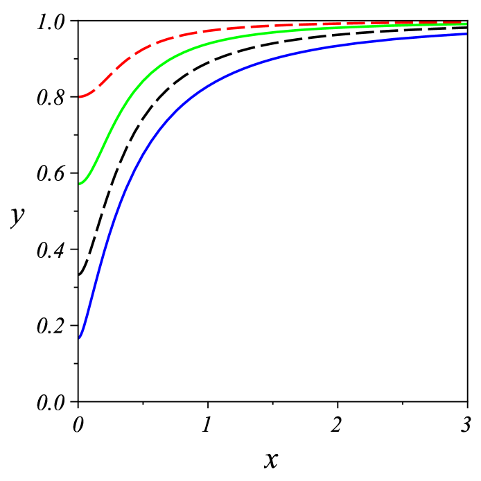
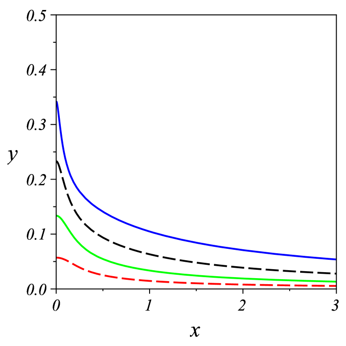
Here k0subscript𝑘0k_{0} is the spring constant of the uncoupled oscillator H^ssubscript^𝐻𝑠\hat{H}_{s}. All effective parameters are now uniquely determined in terms of the starred quantities, namely, Meffsuperscriptsubscript𝑀effM_{\text{\scriptsize eff}}^{\star}, keffsuperscriptsubscript𝑘effk_{\text{\scriptsize eff}}^{\star}, the effective temperature Teff=ωeff/(kBlnξβ)superscriptsubscript𝑇effPlanck-constant-over-2-pisuperscriptsubscript𝜔effsubscript𝑘𝐵subscript𝜉𝛽T_{\text{\scriptsize eff}}^{\star}=-\hbar\omega_{\text{\scriptsize eff}}^{\star}/(k_{B}\,\ln\xi_{\beta}), and the internal energy Ueff=H^effβ(=Us)superscriptsubscript𝑈effannotatedsubscriptdelimited-⟨⟩superscriptsubscript^𝐻eff𝛽absentsubscript𝑈𝑠U_{\text{\scriptsize eff}}^{\star}=\langle\hat{H}_{\text{\scriptsize eff}}^{\star}\rangle_{\beta}\,(=U_{s}) where H^eff=p^2/(2Meff)+(keff/2)q^2superscriptsubscript^𝐻effsuperscript^𝑝22superscriptsubscript𝑀effsuperscriptsubscript𝑘eff2superscript^𝑞2\hat{H}_{\text{\scriptsize eff}}^{\star}=\hat{p}^{2}/(2M_{\text{\scriptsize eff}}^{\star})+(k_{\text{\scriptsize eff}}^{\star}/2)\,\hat{q}^{2} (cf. note, on the other hand, that clearly ρ^s=ρ^eff=ρ^effsubscript^𝜌𝑠subscript^𝜌effsuperscriptsubscript^𝜌eff\hat{\rho}_{s}=\hat{\rho}_{\text{\scriptsize eff}}=\hat{\rho}_{\text{\scriptsize eff}}^{\star}). With the aid of (6) and (7), figure 1 demonstrates that keffk0superscriptsubscript𝑘effsubscript𝑘0k_{\text{\scriptsize eff}}^{\star}\geq k_{0}, which leads to MeffMsuperscriptsubscript𝑀eff𝑀M_{\text{\scriptsize eff}}^{\star}\geq M from Meffkeff=p^2β/q^2βsuperscriptsubscript𝑀effsuperscriptsubscript𝑘effsubscriptdelimited-⟨⟩superscript^𝑝2𝛽subscriptdelimited-⟨⟩superscript^𝑞2𝛽M_{\text{\scriptsize eff}}^{\star}\,k_{\text{\scriptsize eff}}^{\star}=\langle\hat{p}^{2}\rangle_{\beta}/\langle\hat{q}^{2}\rangle_{\beta}. We will use the effective oscillator with (Meff,keff,Teff)superscriptsubscript𝑀effsuperscriptsubscript𝑘effsuperscriptsubscript𝑇eff(M_{\text{\scriptsize eff}}^{\star},k_{\text{\scriptsize eff}}^{\star},T_{\text{\scriptsize eff}}^{\star}) in Section IV for a generalization of the Clausius inequality.

Let us consider the thermal entropy of the effective uncoupled oscillator H^effsubscript^𝐻eff\hat{H}_{\text{\scriptsize eff}} (of course, H^effsuperscriptsubscript^𝐻eff\hat{H}_{\text{\scriptsize eff}}^{\star}, too, as its special case), which is

Seff(=Seff)=kBlnZeff+kBβeffUeff=kB{ln(1ξβ)+ξβ1ξβlnξβ}.annotatedsubscript𝑆effabsentsuperscriptsubscript𝑆effsubscript𝑘𝐵subscript𝑍effsubscript𝑘𝐵subscript𝛽effsubscript𝑈effsubscript𝑘𝐵1subscript𝜉𝛽subscript𝜉𝛽1subscript𝜉𝛽subscript𝜉𝛽\textstyle S_{\text{\scriptsize eff}}\;\left(=S_{\text{\scriptsize eff}}^{\star}\right)\,=\,k_{B}\ln Z_{\text{\scriptsize eff}}\,+\,k_{B}\beta_{\text{\scriptsize eff}}\,U_{\text{\scriptsize eff}}\,=\,-k_{B}\left\{\ln(1-\xi_{\beta})\,+\,\frac{\xi_{\beta}}{1-\xi_{\beta}}\,\ln\xi_{\beta}\right\}\,. (40)

We can immediately verify that this is identical to the von-Neumann entropy of the coupled oscillator,

SN=kB(v+12)ln(v+12)kB(v12)ln(v12)subscript𝑆𝑁subscript𝑘𝐵𝑣12𝑣12subscript𝑘𝐵𝑣12𝑣12S_{N}\,=\,\textstyle k_{B}\left(v+\frac{1}{2}\right)\,\ln\left(v+\frac{1}{2}\right)-k_{B}\left(v-\frac{1}{2}\right)\,\ln\left(v-\frac{1}{2}\right) (41)

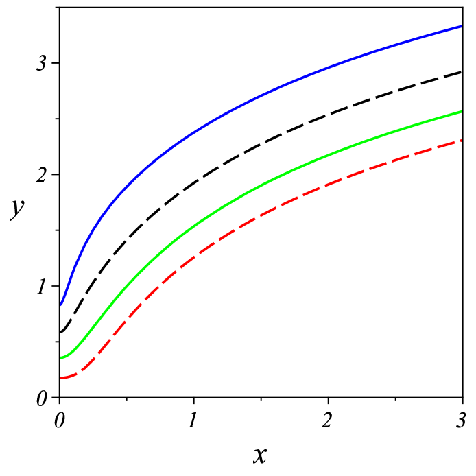
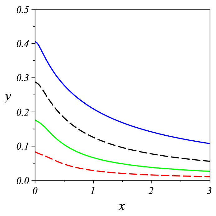
ALL00 (note again that ρ^s=ρ^eff=ρ^effsubscript^𝜌𝑠subscript^𝜌effsuperscriptsubscript^𝜌eff\hat{\rho}_{s}=\hat{\rho}_{\text{\scriptsize eff}}=\hat{\rho}_{\text{\scriptsize eff}}^{\star}). From figure 2, it is shown that SNsubscript𝑆𝑁S_{N} increases with the magnitude of the damping parameter and also with the temperature of the total system.

Now we briefly comment on the introduction of effective parameters: First, it has been shown in SRE93 that the coupled oscillator with (M,ω0)𝑀subscript𝜔0(M,\omega_{0}) at zero temperature of the total system (T=0)𝑇0(T=0) can be interpreted as an uncoupled one with (M,ω¯eff)𝑀subscript¯𝜔eff(M,\bar{\omega}_{\text{\scriptsize eff}}) in a thermal state with a finite effective temperature T¯effsubscript¯𝑇eff\bar{T}_{\text{\scriptsize eff}} (with β=𝛽\beta=\infty), where ω¯eff=p^2/q^2/Msubscript¯𝜔effsubscriptdelimited-⟨⟩superscript^𝑝2subscriptdelimited-⟨⟩superscript^𝑞2𝑀\bar{\omega}_{\text{\scriptsize eff}}=\sqrt{\langle\hat{p}^{2}\rangle_{\infty}/\langle\hat{q}^{2}\rangle_{\infty}}/M. Using the very same technique, we have generalized this result into (Meff,ωeff,Teff)subscript𝑀effsubscript𝜔effsubscript𝑇eff(M_{\text{\scriptsize eff}},\omega_{\text{\scriptsize eff}},T_{\text{\scriptsize eff}}) in (32) and (33) for an arbitrary temperature of the total system. It is interesting to note here that U¯effUs(β=)subscript¯𝑈effsubscript𝑈𝑠𝛽\bar{U}_{\text{\scriptsize eff}}\neq U_{s}(\beta=\infty) though, where U¯eff=p^2/(2M)+{M(ω¯eff)2/2}q^2subscript¯𝑈effsubscriptdelimited-⟨⟩superscript^𝑝22𝑀𝑀superscriptsubscript¯𝜔eff22subscriptdelimited-⟨⟩superscript^𝑞2\bar{U}_{\text{\scriptsize eff}}=\langle\hat{p}^{2}\rangle_{\infty}/(2M)+\{M(\bar{\omega}_{\text{\scriptsize eff}})^{2}/2\}\langle\hat{q}^{2}\rangle_{\infty}. Secondly, it is also known WEI99 ; GRA84 that the coupled oscillator can exactly be seen as an uncoupled oscillator with an effective frequency

ω~eff=2βarccoth(2q^2βp^2β)subscript~𝜔eff2Planck-constant-over-2-pi𝛽arccoth2Planck-constant-over-2-pisubscriptdelimited-⟨⟩superscript^𝑞2𝛽subscriptdelimited-⟨⟩superscript^𝑝2𝛽\textstyle\tilde{\omega}_{\text{\scriptsize eff}}\,=\,\frac{2}{\hbar\beta}\;\mbox{arccoth}\left(\frac{2}{\hbar}\sqrt{\langle\hat{q}^{2}\rangle_{\beta}\,\langle\hat{p}^{2}\rangle_{\beta}}\right) (42)

and an effective mass M~eff=p^2β/q^2β/ω~effsubscript~𝑀effsubscriptdelimited-⟨⟩superscript^𝑝2𝛽subscriptdelimited-⟨⟩superscript^𝑞2𝛽subscript~𝜔eff\tilde{M}_{\text{\scriptsize eff}}=\sqrt{\langle\hat{p}^{2}\rangle_{\beta}/\langle\hat{q}^{2}\rangle_{\beta}}/\tilde{\omega}_{\text{\scriptsize eff}} in the canonical thermal state ρ^s=eβH^s/Zβsubscript^𝜌𝑠superscript𝑒𝛽subscript^𝐻𝑠subscript𝑍𝛽\hat{\rho}_{s}=e^{-\beta\hat{H}_{s}}/Z_{\beta} (i.e., T~eff=Tsubscript~𝑇eff𝑇\tilde{T}_{\text{\scriptsize eff}}=T), which can be well understood simply as a special case of (Meff,ωeff,Teff)subscript𝑀effsubscript𝜔effsubscript𝑇eff(M_{\text{\scriptsize eff}},\omega_{\text{\scriptsize eff}},T_{\text{\scriptsize eff}}) in (32) and (33) (note again that these are not the starred quantities). However, U~effUssubscript~𝑈effsubscript𝑈𝑠\tilde{U}_{\text{\scriptsize eff}}\neq U_{s}, either, whereas Us=Ueffsubscript𝑈𝑠superscriptsubscript𝑈effU_{s}=U_{\text{\scriptsize eff}}^{\star} introduced below equation (38).

It is also interesting to compare the internal energy Ueffsuperscriptsubscript𝑈effU_{\text{\scriptsize eff}}^{\star} of the coupled oscillator with an alternative definition FOR06 ; KIM06 ; KIM07 ; HAE05 ; FOR05 ; HAE06

𝒰=βln𝒵β,𝒰𝛽subscript𝒵𝛽\textstyle{\mathcal{U}}\,=\,-\frac{\partial}{\partial\beta}\,\ln{\mathcal{Z}}_{\beta}\,, (43)

where the partition function 𝒵β=TreβH^/TrbeβH^bsubscript𝒵𝛽Trsuperscript𝑒𝛽^𝐻subscriptTr𝑏superscript𝑒𝛽subscript^𝐻𝑏{\mathcal{Z}}_{\beta}=\mbox{Tr}\,e^{-\beta\hat{H}}/\mbox{Tr}_{b}\,e^{-\beta\hat{H}_{b}}. Here, TrbsubscriptTr𝑏\mbox{Tr}_{b} denotes the partial trace for the bath alone (in the absence of a coupling between system and bath, the function 𝒵βsubscript𝒵𝛽{\mathcal{Z}}_{\beta} would exactly correspond to the partition function of the system only). Then it immediately follows that 𝒰=Us+H^bβ+H^sbβH^bβUs𝒰subscript𝑈𝑠subscriptdelimited-⟨⟩subscript^𝐻𝑏𝛽subscriptdelimited-⟨⟩subscript^𝐻𝑠𝑏𝛽subscriptdelimited-⟨⟩subscript^𝐻𝑏superscript𝛽subscript𝑈𝑠{\mathcal{U}}=U_{s}+\langle\hat{H}_{b}\rangle_{\beta}+\langle\hat{H}_{sb}\rangle_{\beta}-\langle\hat{H}_{b}\rangle_{\beta^{\prime}}\neq U_{s} where H^bβ=Trb(H^beβH^b/TrbeβH^b)subscriptdelimited-⟨⟩subscript^𝐻𝑏superscript𝛽subscriptTr𝑏subscript^𝐻𝑏superscript𝑒𝛽subscript^𝐻𝑏subscriptTr𝑏superscript𝑒𝛽subscript^𝐻𝑏\langle\hat{H}_{b}\rangle_{\beta^{\prime}}=\mbox{Tr}_{b}\left(\hat{H}_{b}\;e^{-\beta\hat{H}_{b}}/\mbox{Tr}_{b}\,e^{-\beta\hat{H}_{b}}\right). Therefore the energy 𝒰𝒰{\mathcal{U}} is not valid for the reduced system alone. The entropy 𝒮=kB(ln𝒵βββln𝒵β)𝒮subscript𝑘𝐵subscript𝒵𝛽𝛽𝛽subscript𝒵𝛽{\mathcal{S}}=k_{B}\,(\ln{\mathcal{Z}}_{\beta}-\beta\,\frac{\partial}{\partial\beta}\ln{\mathcal{Z}}_{\beta}) can also be introduced here FOR05 ; HAE06 , which is, however, different from the von-Neumann entropy SN(=Seff)annotatedsubscript𝑆𝑁absentsuperscriptsubscript𝑆effS_{N}\;(=S_{\text{\scriptsize eff}}^{\star}) for the reduced density matrix ρ^ssubscript^𝜌𝑠\hat{\rho}_{s} of the coupled oscillator. Actually, the entropy 𝒮𝒮{\mathcal{S}} cannot be derived from the Jaynes maximum entropy principle JAY57 ; EJA57 applied for the reduced system whereas the entropy Seffsuperscriptsubscript𝑆effS_{\text{\scriptsize eff}}^{\star} can be so with the effective temperature Teffsuperscriptsubscript𝑇effT_{\text{\scriptsize eff}}^{\star}. As a result, all thermodynamic quantities resulting from the partition function 𝒵βsubscript𝒵𝛽{\mathcal{Z}}_{\beta} are not appropriate for the well-defined local thermodynamics of the reduced system.

IV Clausius inequalities

We will discuss the second law of thermodynamics in terms of the Clausius inequality. To do so, we need the relationship obtained from (23),

dUs=n(Endpn+pndEn)𝑑subscript𝑈𝑠subscript𝑛subscript𝐸𝑛𝑑subscript𝑝𝑛subscript𝑝𝑛𝑑subscript𝐸𝑛dU_{s}\,=\,\sum_{n}\textstyle\left(E_{n}\,dp_{n}\,+\,p_{n}\,dE_{n}\right) (44)

where Endpn=Trs(H^sdρ^s)=δ𝒬ssubscript𝐸𝑛𝑑subscript𝑝𝑛subscriptTr𝑠subscript^𝐻𝑠𝑑subscript^𝜌𝑠𝛿subscript𝒬𝑠\sum E_{n}dp_{n}=\mbox{Tr}_{s}(\hat{H}_{s}\,d\hat{\rho}_{s})=\delta{\mathcal{Q}}_{s} corresponds to an amount of heat added to the coupled oscillator, and pndEn=Trs(ρ^sdH^s)=δ𝒲ssubscript𝑝𝑛𝑑subscript𝐸𝑛subscriptTr𝑠subscript^𝜌𝑠𝑑subscript^𝐻𝑠𝛿subscript𝒲𝑠\sum p_{n}dE_{n}=\mbox{Tr}_{s}(\hat{\rho}_{s}\,d\hat{H}_{s})=\delta{\mathcal{W}}_{s} an amount of work on the oscillator ALL00 . For a later purpose, we first consider the well-defined Clausius inequality for a weakly coupled oscillator

δ𝒬sTdS.𝛿subscript𝒬𝑠𝑇𝑑𝑆\textstyle\delta{\mathcal{Q}}_{s}\leq T\,dS\,. (45)

For a typical reversible process we have either a variation of the mass of the oscillator or a variation of its spring constant in such a way that

M𝒬s𝑀subscript𝒬𝑠\displaystyle\textstyle\frac{\partial}{\partial M}{\mathcal{Q}}_{s} =\displaystyle= 12MMp^2β+k02Mq^2β12𝑀𝑀subscriptdelimited-⟨⟩superscript^𝑝2𝛽subscript𝑘02𝑀subscriptdelimited-⟨⟩superscript^𝑞2𝛽\displaystyle\textstyle\frac{1}{2M}\frac{\partial}{\partial M}\langle\hat{p}^{2}\rangle_{\beta}\,+\,\frac{k_{0}}{2}\frac{\partial}{\partial M}\langle\hat{q}^{2}\rangle_{\beta} (46)
=\displaystyle= β(ω0)28M(cschβω02)2=TMS𝛽superscriptPlanck-constant-over-2-pisubscript𝜔028𝑀superscriptcsch𝛽Planck-constant-over-2-pisubscript𝜔022𝑇𝑀𝑆\displaystyle\textstyle\frac{\beta\,(\hbar\omega_{0})^{2}}{8M}\,\left(\text{csch}\frac{\beta\hbar\omega_{0}}{2}\right)^{2}\,=\,T\,\frac{\partial}{\partial M}S (47)
k0𝒬ssubscript𝑘0subscript𝒬𝑠\displaystyle\textstyle\frac{\partial}{\partial k_{0}}{\mathcal{Q}}_{s} =\displaystyle= 12Mk0p^2β+k02k0q^2β12𝑀subscript𝑘0subscriptdelimited-⟨⟩superscript^𝑝2𝛽subscript𝑘02subscript𝑘0subscriptdelimited-⟨⟩superscript^𝑞2𝛽\displaystyle\textstyle\frac{1}{2M}\frac{\partial}{\partial k_{0}}\langle\hat{p}^{2}\rangle_{\beta}\,+\,\frac{k_{0}}{2}\frac{\partial}{\partial k_{0}}\langle\hat{q}^{2}\rangle_{\beta} (48)
=\displaystyle= β28M(cschβω02)2=Tk0S,𝛽superscriptPlanck-constant-over-2-pi28𝑀superscriptcsch𝛽Planck-constant-over-2-pisubscript𝜔022𝑇subscript𝑘0𝑆\displaystyle\textstyle-\frac{\beta\,\hbar^{2}}{8M}\,\left(\text{csch}\frac{\beta\hbar\omega_{0}}{2}\right)^{2}\,=\,T\,\frac{\partial}{\partial k_{0}}S\,, (49)

respectively (cf. it is also noted that 𝒲s/M=p^2β/(2M2)subscript𝒲𝑠𝑀subscriptdelimited-⟨⟩superscript^𝑝2𝛽2superscript𝑀2\partial{\mathcal{W}}_{s}/\partial M=-\langle\hat{p}^{2}\rangle_{\beta}/(2M^{2}) and 𝒲s/k0=q^2β/2subscript𝒲𝑠subscript𝑘0subscriptdelimited-⟨⟩superscript^𝑞2𝛽2\partial{\mathcal{W}}_{s}/\partial k_{0}=\langle\hat{q}^{2}\rangle_{\beta}/2). We thus confirm the equality sign in equation (45).

Next we consider the Clausius inequality in the process of coupling between oscillator and bath. The coupling process can be represented in terms of a variation of the damping parameter such that for a reversible process,

γ𝒬s𝛾subscript𝒬𝑠\displaystyle\textstyle\frac{\partial}{\partial\gamma}{\mathcal{Q}}_{s} =\displaystyle= γUs=12Mγp^2β+k02γq^2β𝛾subscript𝑈𝑠12𝑀𝛾subscriptdelimited-⟨⟩superscript^𝑝2𝛽subscript𝑘02𝛾subscriptdelimited-⟨⟩superscript^𝑞2𝛽\displaystyle\textstyle\frac{\partial}{\partial\gamma}U_{s}\,=\,\frac{1}{2M}\frac{\partial}{\partial\gamma}\langle\hat{p}^{2}\rangle_{\beta}\,+\,\frac{k_{0}}{2}\frac{\partial}{\partial\gamma}\langle\hat{q}^{2}\rangle_{\beta} (50)
γS𝛾𝑆\displaystyle\textstyle\frac{\partial}{\partial\gamma}S =\displaystyle= kB(vγ)lnv+12v12subscript𝑘𝐵𝑣𝛾𝑣12𝑣12\displaystyle\textstyle k_{B}\left(\frac{\partial v}{\partial\gamma}\right)\,\ln\frac{v+\frac{1}{2}}{v-\frac{1}{2}} (51)

where S=SN𝑆subscript𝑆𝑁S=S_{N} and

vγ=12q^2βγp^2β+p^2βγq^2βq^2βp^2β.𝑣𝛾12Planck-constant-over-2-pisubscriptdelimited-⟨⟩superscript^𝑞2𝛽𝛾subscriptdelimited-⟨⟩superscript^𝑝2𝛽subscriptdelimited-⟨⟩superscript^𝑝2𝛽𝛾subscriptdelimited-⟨⟩superscript^𝑞2𝛽subscriptdelimited-⟨⟩superscript^𝑞2𝛽subscriptdelimited-⟨⟩superscript^𝑝2𝛽\textstyle\frac{\partial v}{\partial\gamma}\,=\,\frac{1}{2\hbar}\frac{\langle\hat{q}^{2}\rangle_{\beta}\,\frac{\partial}{\partial\gamma}\langle\hat{p}^{2}\rangle_{\beta}\,+\,\langle\hat{p}^{2}\rangle_{\beta}\,\frac{\partial}{\partial\gamma}\langle\hat{q}^{2}\rangle_{\beta}}{\sqrt{\langle\hat{q}^{2}\rangle_{\beta}\,\langle\hat{p}^{2}\rangle_{\beta}}}\,. (52)

Equation (50) can be evaluated in closed form with the aid of equations (6)-(9) such that

γq^2β(d)𝛾superscriptsubscriptdelimited-⟨⟩superscript^𝑞2𝛽𝑑\displaystyle\textstyle\frac{\partial}{\partial\gamma}\langle\hat{q}^{2}\rangle_{\beta}^{(d)} =\displaystyle= 1Ml=13Kl(d)γ1𝑀superscriptsubscript𝑙13subscriptsuperscriptsubscript𝐾𝑙𝑑𝛾\displaystyle{\textstyle\frac{1}{M}}\sum_{l=1}^{3}{}_{\gamma}K_{l}^{(d)} (53)
γp^2β(d)𝛾superscriptsubscriptdelimited-⟨⟩superscript^𝑝2𝛽𝑑\displaystyle\textstyle\frac{\partial}{\partial\gamma}\langle\hat{p}^{2}\rangle_{\beta}^{(d)} =\displaystyle= Ml=13(Kl(d)γωl¯2+ 2ωl¯λd(l){1βωl¯+πψ(βωl¯2π)}ωl¯γ)𝑀superscriptsubscript𝑙13subscriptsuperscriptsubscript𝐾𝑙𝑑𝛾superscript¯subscript𝜔𝑙22¯subscript𝜔𝑙superscriptsubscript𝜆𝑑𝑙1𝛽¯subscript𝜔𝑙Planck-constant-over-2-pi𝜋𝜓𝛽Planck-constant-over-2-pi¯subscript𝜔𝑙2𝜋¯subscript𝜔𝑙𝛾\displaystyle-M\sum_{l=1}^{3}\textstyle\left({}_{\gamma}K_{l}^{(d)}\underline{\omega_{l}}^{2}\,+\,2\underline{\omega_{l}}\,\lambda_{d}^{(l)}\left\{\frac{1}{\beta\underline{\omega_{l}}}\,+\,\frac{\hbar}{\pi}\;\psi\left(\frac{\beta\hbar\underline{\omega_{l}}}{2\pi}\right)\right\}\frac{\partial\underline{\omega_{l}}}{\partial\gamma}\right) (54)

where ω1¯/γ=0¯subscript𝜔1𝛾0\partial\underline{\omega_{1}}/\partial\gamma=0 and

ω2¯γ=12(111(2𝐰0γ)2);ω3¯γ=12(1+11(2𝐰0γ)2),formulae-sequence¯subscript𝜔2𝛾12111superscript2subscript𝐰0𝛾2¯subscript𝜔3𝛾12111superscript2subscript𝐰0𝛾2\textstyle\frac{\partial\underline{\omega_{2}}}{\partial\gamma}\,=\,\frac{1}{2}\left(1-\frac{1}{\sqrt{1-\left(\frac{2{\mathbf{w}}_{0}}{\gamma}\right)^{2}}}\right)\;;\;\frac{\partial\underline{\omega_{3}}}{\partial\gamma}\,=\,\frac{1}{2}\left(1+\frac{1}{\sqrt{1-\left(\frac{2{\mathbf{w}}_{0}}{\gamma}\right)^{2}}}\right)\,, (55)

and

Kl(d)γ={1βωl¯+πψ(βωl¯2π)}λd(l)γ+λd(l){1βωl¯2+2β2π2ψ(1)(βωl¯2π)}ωl¯γsubscriptsuperscriptsubscript𝐾𝑙𝑑𝛾1𝛽¯subscript𝜔𝑙Planck-constant-over-2-pi𝜋𝜓𝛽Planck-constant-over-2-pi¯subscript𝜔𝑙2𝜋superscriptsubscript𝜆𝑑𝑙𝛾superscriptsubscript𝜆𝑑𝑙1𝛽superscript¯subscript𝜔𝑙2superscriptPlanck-constant-over-2-pi2𝛽2superscript𝜋2superscript𝜓1𝛽Planck-constant-over-2-pi¯subscript𝜔𝑙2𝜋¯subscript𝜔𝑙𝛾\textstyle{}_{\gamma}K_{l}^{(d)}\,=\,\left\{\frac{1}{\beta\underline{\omega_{l}}}\,+\,\frac{\hbar}{\pi}\;\psi\left(\frac{\beta\hbar\underline{\omega_{l}}}{2\pi}\right)\right\}\frac{\partial\lambda_{d}^{(l)}}{\partial\gamma}\,+\,\lambda_{d}^{(l)}\,\left\{-\frac{1}{\beta\underline{\omega_{l}}^{2}}\,+\,\frac{\hbar^{2}\beta}{2\pi^{2}}\;\psi^{(1)}(\frac{\beta\hbar\underline{\omega_{l}}}{2\pi})\right\}\frac{\partial\underline{\omega_{l}}}{\partial\gamma} (56)

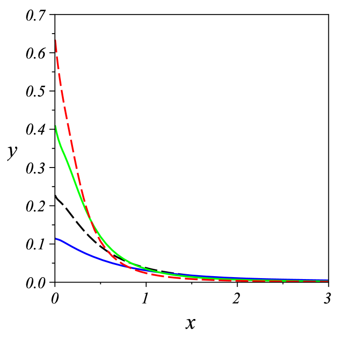
in terms of the digamma function ψ(y)𝜓𝑦\psi(y) and the trigamma function ψ(1)(y)=d2lnΓ(y)/dy2superscript𝜓1𝑦superscript𝑑2Γ𝑦𝑑superscript𝑦2\psi^{(1)}(y)=d^{2}\ln\Gamma(y)/dy^{2} ABS74 . Here we obtained equations (53) and (54) for the overdamped case (γ/2>𝐰0)𝛾2subscript𝐰0(\gamma/2>{\mathbf{w}}_{0}), which is, still, found to hold for the underdamped case (γ/2𝐰0)𝛾2subscript𝐰0(\gamma/2\leq{\mathbf{w}}_{0}) as well, being expressed in terms of the functions with complex-valued arguments. Then we get a violation of the Clausius inequality, 𝒬s/γ>TSN/γsubscript𝒬𝑠𝛾𝑇subscript𝑆𝑁𝛾\partial{\mathcal{Q}}_{s}/\partial\gamma>T\,\partial S_{N}/\partial\gamma as seen from figure 3.

We, however, argue that this violation results from an inappropriate choice of temperature T𝑇T being defined for the total system. We now propose a well-defined form of the Clausius inequality pertaining to the coupling process in such a way that

δ𝒬effTeffdSN𝛿superscriptsubscript𝒬effsuperscriptsubscript𝑇eff𝑑subscript𝑆𝑁\textstyle\delta{\mathcal{Q}}_{\text{\scriptsize eff}}^{\star}\,\leq\,T_{\text{\scriptsize eff}}^{\star}\,dS_{N} (57)

where δ𝒬eff𝛿superscriptsubscript𝒬eff\delta{\mathcal{Q}}_{\text{\scriptsize eff}}^{\star} is the heat exchanged between the effective (weakly coupled) oscillator with (Meff,keff)superscriptsubscript𝑀effsuperscriptsubscript𝑘eff(M_{\text{\scriptsize eff}}^{\star},k_{\text{\scriptsize eff}}^{\star}) in (39) and a bath at the equilibrium temperature Teff=ωeff/(kBlnξβ)superscriptsubscript𝑇effPlanck-constant-over-2-pisuperscriptsubscript𝜔effsubscript𝑘𝐵subscript𝜉𝛽T_{\text{\scriptsize eff}}^{\star}=-\hbar\omega_{\text{\scriptsize eff}}^{\star}/(k_{B}\ln\xi_{\beta}) with (38). For an reversible process we then have

γ𝒬eff=12Meffγp^2β+keff2γq^2β,𝛾superscriptsubscript𝒬eff12superscriptsubscript𝑀eff𝛾subscriptdelimited-⟨⟩superscript^𝑝2𝛽superscriptsubscript𝑘eff2𝛾subscriptdelimited-⟨⟩superscript^𝑞2𝛽\textstyle\frac{\partial}{\partial\gamma}{\mathcal{Q}}_{\text{\scriptsize eff}}^{\star}\,=\,\frac{1}{2M_{\text{\scriptsize eff}}^{\star}}\,\frac{\partial}{\partial\gamma}\langle\hat{p}^{2}\rangle_{\beta}\,+\,\frac{k_{\text{\scriptsize eff}}^{\star}}{2}\frac{\partial}{\partial\gamma}\langle\hat{q}^{2}\rangle_{\beta}\,, (58)

which can be shown to be identical to TeffSN/γsuperscriptsubscript𝑇effsubscript𝑆𝑁𝛾T_{\text{\scriptsize eff}}^{\star}\,\partial S_{N}/\partial\gamma with the aid of (51) and (52). Therefore, there is no violation of the Clausius inequality! From Ueff=Ussuperscriptsubscript𝑈effsubscript𝑈𝑠U_{\text{\scriptsize eff}}^{\star}=U_{s}, we note that 0γ𝑑Ueff=0γ𝑑Us=Us(γ)U0=ΔUssuperscriptsubscript0𝛾differential-dsuperscriptsubscript𝑈effsuperscriptsubscript0𝛾differential-dsubscript𝑈𝑠subscript𝑈𝑠𝛾subscript𝑈0Δsubscript𝑈𝑠\int_{0}^{\gamma}dU_{\text{\scriptsize eff}}^{\star}=\int_{0}^{\gamma}dU_{s}=U_{s}(\gamma)-U_{0}=\Delta U_{s}, in which U0=(ω0/2)coth(βω0/2)subscript𝑈0Planck-constant-over-2-pisubscript𝜔02hyperbolic-cotangent𝛽Planck-constant-over-2-pisubscript𝜔02U_{0}=(\hbar\omega_{0}/2)\coth(\beta\hbar\omega_{0}/2) for an uncoupled oscillator, and 𝑑Us=𝑑Ueff=0contour-integraldifferential-dsubscript𝑈𝑠contour-integraldifferential-dsuperscriptsubscript𝑈eff0\oint dU_{s}=\oint dU_{\text{\scriptsize eff}}^{\star}=0, where =0γ+γ0contour-integralsuperscriptsubscript0𝛾superscriptsubscript𝛾0\oint=\int_{0}^{\gamma}+\int_{\gamma}^{0} represents a cyclic process of the coupling and decoupling. From the first law dUs=δ𝒬s+δ𝒲s=δ𝒬eff+δ𝒲eff𝑑subscript𝑈𝑠𝛿subscript𝒬𝑠𝛿subscript𝒲𝑠𝛿superscriptsubscript𝒬eff𝛿superscriptsubscript𝒲effdU_{s}=\delta{\mathcal{Q}}_{s}+\delta{\mathcal{W}}_{s}=\delta{\mathcal{Q}}_{\text{\scriptsize eff}}^{\star}+\delta{\mathcal{W}}_{\text{\scriptsize eff}}^{\star} with 𝒲s/γ=0subscript𝒲𝑠𝛾0\partial{\mathcal{W}}_{s}/\partial\gamma=0 and thus (𝒬eff𝒬s)/γ=𝒲eff/γsuperscriptsubscript𝒬effsubscript𝒬𝑠𝛾superscriptsubscript𝒲eff𝛾\partial({\mathcal{Q}}_{\text{\scriptsize eff}}^{\star}-{\mathcal{Q}}_{s})/\partial\gamma=-\partial{\mathcal{W}}_{\text{\scriptsize eff}}^{\star}/\partial\gamma, it also follows that

γ𝒬sγ𝒲eff=TeffγSN𝛾subscript𝒬𝑠𝛾superscriptsubscript𝒲effsuperscriptsubscript𝑇eff𝛾subscript𝑆𝑁\textstyle\frac{\partial}{\partial\gamma}{\mathcal{Q}}_{s}\,-\,\frac{\partial}{\partial\gamma}{\mathcal{W}}_{\text{\scriptsize eff}}^{\star}\,=\,T_{\text{\scriptsize eff}}^{\star}\,\frac{\partial}{\partial\gamma}S_{N} (59)

where, with the aid of (39),

γ𝒲eff𝛾superscriptsubscript𝒲eff\displaystyle\textstyle\frac{\partial}{\partial\gamma}{\mathcal{W}}_{\text{\scriptsize eff}}^{\star} =\displaystyle= 12Meff(Meffγ)p^2β+12(keffγ)q^2β12superscriptsubscript𝑀effsuperscriptsubscript𝑀eff𝛾subscriptdelimited-⟨⟩superscript^𝑝2𝛽12superscriptsubscript𝑘eff𝛾subscriptdelimited-⟨⟩superscript^𝑞2𝛽\displaystyle\textstyle-\frac{1}{2M_{\text{\scriptsize eff}}^{\star}}\left(\frac{\partial M_{\text{\scriptsize eff}}^{\star}}{\partial\gamma}\right)\langle\hat{p}^{2}\rangle_{\beta}\,+\,\frac{1}{2}\left(\frac{\partial k_{\text{\scriptsize eff}}^{\star}}{\partial\gamma}\right)\langle\hat{q}^{2}\rangle_{\beta} (60)
=\displaystyle= 14M(1Mk0q^2βp^2β)γp^2β+k04(1p^2βMk0q^2β)γq^2β.14𝑀1𝑀subscript𝑘0subscriptdelimited-⟨⟩superscript^𝑞2𝛽subscriptdelimited-⟨⟩superscript^𝑝2𝛽𝛾subscriptdelimited-⟨⟩superscript^𝑝2𝛽subscript𝑘041subscriptdelimited-⟨⟩superscript^𝑝2𝛽𝑀subscript𝑘0subscriptdelimited-⟨⟩superscript^𝑞2𝛽𝛾subscriptdelimited-⟨⟩superscript^𝑞2𝛽\displaystyle\textstyle\frac{1}{4M}\left(1-\frac{Mk_{0}\,\langle\hat{q}^{2}\rangle_{\beta}}{\langle\hat{p}^{2}\rangle_{\beta}}\right)\frac{\partial}{\partial\gamma}\langle\hat{p}^{2}\rangle_{\beta}\,+\,\frac{k_{0}}{4}\left(1-\frac{\langle\hat{p}^{2}\rangle_{\beta}}{Mk_{0}\,\langle\hat{q}^{2}\rangle_{\beta}}\right)\frac{\partial}{\partial\gamma}\langle\hat{q}^{2}\rangle_{\beta}\,.

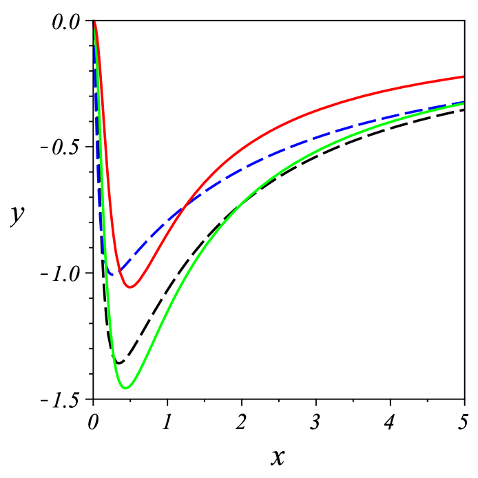
Figure 4 shows that 𝒲eff/γ0superscriptsubscript𝒲eff𝛾0\partial{\mathcal{W}}_{\text{\scriptsize eff}}^{\star}/\partial\gamma\leq 0, which immediately leads to no violation of the inequality 𝒬s/γTeffSN/γsubscript𝒬𝑠𝛾superscriptsubscript𝑇effsubscript𝑆𝑁𝛾\partial{\mathcal{Q}}_{s}/\partial\gamma\leq T_{\text{\scriptsize eff}}^{\star}\,\partial S_{N}/\partial\gamma. Here it should be noted that we have appropriately selected the effective oscillator H^effsuperscriptsubscript^𝐻eff\hat{H}_{\text{\scriptsize eff}}^{\star} with (Meff,ωeff)superscriptsubscript𝑀effsuperscriptsubscript𝜔eff(M_{\text{\scriptsize eff}}^{\star},\omega_{\text{\scriptsize eff}}^{\star}) from (32) to introduce an effective temperature Teffsuperscriptsubscript𝑇effT_{\text{\scriptsize eff}}^{\star} without any ambiguity, which is now a critical element for the well-defined Clausius inequality in (57).

Therefore, we are now in a position to understand, by means of the Clausius inequality (57), the validity of the second law in a cyclic process of the coupling and decoupling between oscillator and bath at an equilibrium temperature T𝑇T. The validity has actually been shown for zero temperature (T=0)𝑇0(T=0) in FOR06 ; KIM06 and later for an arbitrary temperature in KIM07 by verifying the second law in its Kelvin-Planck form ANN02 ; it states that the minimum work ΔΔ\Delta{\mathcal{F}} needed to couple the oscillator to a bath (in a reversible process), being equivalent to the Helmholtz free energy of the coupled total system minus the free energy of the uncoupled total system, cannot be less than the maximum useful work obtainable from the oscillator when it decouples from the bath such that

ΔUsΔless-than-and-not-equalsΔsubscript𝑈𝑠Δ\textstyle\Delta U_{s}\,\lneq\,\Delta{\mathcal{F}} (61)

(note the strict inequality and see below). Here we have on the left hand side the internal energy ΔUsΔsubscript𝑈𝑠\Delta U_{s} as the maximum useful work obtainable from the oscillator on completion of the decoupling process.

For the coupling-decoupling process (with a varying damping parameter γ:0γ0:superscript𝛾0𝛾0\gamma^{\prime}:0\to\gamma\to 0), inequality (57) can be transformed to δ𝒬eff/Teff0contour-integral𝛿superscriptsubscript𝒬effsuperscriptsubscript𝑇eff0\oint\delta{\mathcal{Q}}_{\text{\scriptsize eff}}^{\star}/T_{\text{\scriptsize eff}}^{\star}\leq 0, which means, according to the Kelvin-Planck form, that the net work obtainable from the effective uncoupled oscillator (with an accordingly varying parameter γsuperscript𝛾\gamma^{\prime}) on completion of this cyclic process cannot be greater than zero. For a reversible process, this inequality then reduces to

0γdγTeffγ𝒬eff+γ0dγTeffγ𝒬eff= 0,superscriptsubscript0𝛾𝑑superscript𝛾superscriptsubscript𝑇effsuperscript𝛾superscriptsubscript𝒬effsuperscriptsubscript𝛾0𝑑superscript𝛾superscriptsubscript𝑇effsuperscript𝛾superscriptsubscript𝒬eff 0\textstyle\int_{0}^{\gamma}\frac{d\gamma^{\prime}}{T_{\text{\scriptsize eff}}^{\star}}\,\frac{\partial}{\partial\gamma^{\prime}}{\mathcal{Q}}_{\text{\scriptsize eff}}^{\star}\,+\,\int_{\gamma}^{0}\frac{d\gamma^{\prime}}{T_{\text{\scriptsize eff}}^{\star}}\,\frac{\partial}{\partial\gamma^{\prime}}{\mathcal{Q}}_{\text{\scriptsize eff}}^{\star}\,=\,0\,, (62)

which means that the minimum work (ΔUs)Δsubscript𝑈𝑠(\Delta U_{s}) done onto the oscillator for U0Ueffsubscript𝑈0superscriptsubscript𝑈effU_{0}\to U_{\text{\scriptsize eff}}^{\star} on completion of the coupling exactly equals the maximum useful work releasable from the oscillator on completion of the decoupling. For comparison, on the other hand, the free energy ΔΔ\Delta{\mathcal{F}} is, by definition, the minimum work done on both oscillator and bath so that we get the inequality in (61). Anyhow, the second law holds in the coupling-decoupling process.

Now we consider the Clausius inequality (with a fixed coupling strength) after completion of the coupling, which has been discussed so far, e.g., in ALL00 ; NIE02 ; LUT08 . Note that we are now with the effective oscillator with (Meff,keff)superscriptsubscript𝑀effsuperscriptsubscript𝑘eff(M_{\text{\scriptsize eff}}^{\star},k_{\text{\scriptsize eff}}^{\star}) at temperature Teffsuperscriptsubscript𝑇effT_{\text{\scriptsize eff}}^{\star}. We can then show that for a reversible process,

M𝒬eff𝑀superscriptsubscript𝒬eff\displaystyle\textstyle\frac{\partial}{\partial M}{\mathcal{Q}}_{\text{\scriptsize eff}}^{\star} =\displaystyle= 12MeffMp^2β+keff2Mq^2β=ωeff4(Mlnξβ)(cschlnξβ2)2=TeffMSN12superscriptsubscript𝑀eff𝑀subscriptdelimited-⟨⟩superscript^𝑝2𝛽superscriptsubscript𝑘eff2𝑀subscriptdelimited-⟨⟩superscript^𝑞2𝛽Planck-constant-over-2-pisuperscriptsubscript𝜔eff4𝑀subscript𝜉𝛽superscriptcschsubscript𝜉𝛽22superscriptsubscript𝑇eff𝑀subscript𝑆𝑁\displaystyle\textstyle\frac{1}{2M_{\text{\scriptsize eff}}^{\star}}\frac{\partial}{\partial M}\langle\hat{p}^{2}\rangle_{\beta}\,+\,\frac{k_{\text{\scriptsize eff}}^{\star}}{2}\frac{\partial}{\partial M}\langle\hat{q}^{2}\rangle_{\beta}\,=\,\frac{\hbar\omega_{\text{\scriptsize eff}}^{\star}}{4}\left(\frac{\partial}{\partial M}\ln\xi_{\beta}\right)\left(\text{csch}\frac{\ln\xi_{\beta}}{2}\right)^{2}\,=\,T_{\text{\scriptsize eff}}^{\star}\,\frac{\partial}{\partial M}S_{N} (63)
k0𝒬effsubscript𝑘0superscriptsubscript𝒬eff\displaystyle\textstyle\frac{\partial}{\partial k_{0}}{\mathcal{Q}}_{\text{\scriptsize eff}}^{\star} =\displaystyle= 12Meffk0p^2β+keff2k0q^2β=ωeff4(k0lnξβ)(cschlnξβ2)2=Teffk0SN,12superscriptsubscript𝑀effsubscript𝑘0subscriptdelimited-⟨⟩superscript^𝑝2𝛽superscriptsubscript𝑘eff2subscript𝑘0subscriptdelimited-⟨⟩superscript^𝑞2𝛽Planck-constant-over-2-pisuperscriptsubscript𝜔eff4subscript𝑘0subscript𝜉𝛽superscriptcschsubscript𝜉𝛽22superscriptsubscript𝑇effsubscript𝑘0subscript𝑆𝑁\displaystyle\textstyle\frac{1}{2M_{\text{\scriptsize eff}}^{\star}}\frac{\partial}{\partial k_{0}}\langle\hat{p}^{2}\rangle_{\beta}\,+\,\frac{k_{\text{\scriptsize eff}}^{\star}}{2}\frac{\partial}{\partial k_{0}}\langle\hat{q}^{2}\rangle_{\beta}\,=\,\frac{\hbar\omega_{\text{\scriptsize eff}}^{\star}}{4}\left(\frac{\partial}{\partial k_{0}}\ln\xi_{\beta}\right)\left(\text{csch}\frac{\ln\xi_{\beta}}{2}\right)^{2}\,=\,T_{\text{\scriptsize eff}}^{\star}\,\frac{\partial}{\partial k_{0}}S_{N}\,, (64)

which follow from (33), (36), (38) and (39), respectively. Therefore, there is no violation of the Clausius inequality at all! Note here as well that from the first law dUs=δ𝒬s+δ𝒲s=δ𝒬eff+δ𝒲eff𝑑subscript𝑈𝑠𝛿subscript𝒬𝑠𝛿subscript𝒲𝑠𝛿superscriptsubscript𝒬eff𝛿superscriptsubscript𝒲effdU_{s}=\delta{\mathcal{Q}}_{s}+\delta{\mathcal{W}}_{s}=\delta{\mathcal{Q}}_{\text{\scriptsize eff}}^{\star}+\delta{\mathcal{W}}_{\text{\scriptsize eff}}^{\star}, the effective work is also well-defined such as

M,k0𝒲eff=12Meff(M,k0Meff)p^2β+12(M,k0keff)q^2β,subscript𝑀subscript𝑘0superscriptsubscript𝒲eff12superscriptsubscript𝑀effsubscript𝑀subscript𝑘0superscriptsubscript𝑀effsubscriptdelimited-⟨⟩superscript^𝑝2𝛽12subscript𝑀subscript𝑘0superscriptsubscript𝑘effsubscriptdelimited-⟨⟩superscript^𝑞2𝛽\textstyle\partial_{M,k_{0}}{\mathcal{W}}_{\text{\scriptsize eff}}^{\star}\,=\,-\frac{1}{2M_{\text{\scriptsize eff}}^{\star}}\left(\partial_{M,k_{0}}M_{\text{\scriptsize eff}}^{\star}\right)\langle\hat{p}^{2}\rangle_{\beta}\,+\,\frac{1}{2}\left(\partial_{M,k_{0}}k_{\text{\scriptsize eff}}^{\star}\right)\langle\hat{q}^{2}\rangle_{\beta}\,, (65)

the closed form of which can immediately be obtained with the aid of Meff=p^2β/Ussuperscriptsubscript𝑀effsubscriptdelimited-⟨⟩superscript^𝑝2𝛽subscript𝑈𝑠M_{\text{\scriptsize eff}}^{\star}=\langle\hat{p}^{2}\rangle_{\beta}/U_{s} and (39).

For comparison, we next seek to have equations (46) and (48) in closed form in the Drude damping model. After making some lengthy calculations (cf. Appendix B), we then obtain the expressions

Mq^2β(d)𝑀superscriptsubscriptdelimited-⟨⟩superscript^𝑞2𝛽𝑑\displaystyle\textstyle\frac{\partial}{\partial M}\langle\hat{q}^{2}\rangle_{\beta}^{(d)} =\displaystyle= 1Mq^2β(d)+1Ml=13Kl(d)M1𝑀superscriptsubscriptdelimited-⟨⟩superscript^𝑞2𝛽𝑑1𝑀superscriptsubscript𝑙13subscriptsuperscriptsubscript𝐾𝑙𝑑𝑀\displaystyle{\textstyle-\frac{1}{M}\langle\hat{q}^{2}\rangle_{\beta}^{(d)}\,+\,\frac{1}{M}}\sum_{l=1}^{3}{}_{M}K_{l}^{(d)} (66)
Mp^2β(d)𝑀superscriptsubscriptdelimited-⟨⟩superscript^𝑝2𝛽𝑑\displaystyle\textstyle\frac{\partial}{\partial M}\langle\hat{p}^{2}\rangle_{\beta}^{(d)} =\displaystyle= 1Mp^2β(d)Ml=13(Kl(d)Mωl¯2+ 2ωl¯λd(l){1βωl¯+πψ(βωl¯2π)}ωl¯M)1𝑀superscriptsubscriptdelimited-⟨⟩superscript^𝑝2𝛽𝑑𝑀superscriptsubscript𝑙13subscriptsuperscriptsubscript𝐾𝑙𝑑𝑀superscript¯subscript𝜔𝑙22¯subscript𝜔𝑙superscriptsubscript𝜆𝑑𝑙1𝛽¯subscript𝜔𝑙Planck-constant-over-2-pi𝜋𝜓𝛽Planck-constant-over-2-pi¯subscript𝜔𝑙2𝜋¯subscript𝜔𝑙𝑀\displaystyle{\textstyle\frac{1}{M}\langle\hat{p}^{2}\rangle_{\beta}^{(d)}}-M\sum_{l=1}^{3}\textstyle\left({}_{M}K_{l}^{(d)}\underline{\omega_{l}}^{2}\,+\,2\underline{\omega_{l}}\,\lambda_{d}^{(l)}\left\{\frac{1}{\beta\underline{\omega_{l}}}\,+\,\frac{\hbar}{\pi}\;\psi\left(\frac{\beta\hbar\underline{\omega_{l}}}{2\pi}\right)\right\}\frac{\partial\underline{\omega_{l}}}{\partial M}\right) (67)

where

Kl(d)M:={1βωl¯+πψ(βωl¯2π)}λd(l)M+λd(l){1βωl¯2+2β2π2ψ(1)(βωl¯2π)}ωl¯M,assignsubscriptsuperscriptsubscript𝐾𝑙𝑑𝑀1𝛽¯subscript𝜔𝑙Planck-constant-over-2-pi𝜋𝜓𝛽Planck-constant-over-2-pi¯subscript𝜔𝑙2𝜋superscriptsubscript𝜆𝑑𝑙𝑀superscriptsubscript𝜆𝑑𝑙1𝛽superscript¯subscript𝜔𝑙2superscriptPlanck-constant-over-2-pi2𝛽2superscript𝜋2superscript𝜓1𝛽Planck-constant-over-2-pi¯subscript𝜔𝑙2𝜋¯subscript𝜔𝑙𝑀\textstyle{}_{M}K_{l}^{(d)}:=\left\{\frac{1}{\beta\underline{\omega_{l}}}\,+\,\frac{\hbar}{\pi}\;\psi\left(\frac{\beta\hbar\underline{\omega_{l}}}{2\pi}\right)\right\}\frac{\partial\lambda_{d}^{(l)}}{\partial M}\,+\,\lambda_{d}^{(l)}\,\left\{-\frac{1}{\beta\underline{\omega_{l}}^{2}}\,+\,\frac{\hbar^{2}\beta}{2\pi^{2}}\;\psi^{(1)}(\frac{\beta\hbar\underline{\omega_{l}}}{2\pi})\right\}\frac{\partial\underline{\omega_{l}}}{\partial M}\,, (68)

and

k0q^2β(d)subscript𝑘0superscriptsubscriptdelimited-⟨⟩superscript^𝑞2𝛽𝑑\displaystyle\textstyle\frac{\partial}{\partial k_{0}}\langle\hat{q}^{2}\rangle_{\beta}^{(d)} =\displaystyle= 1Ml=13Kl(d)k01𝑀superscriptsubscript𝑙13subscriptsuperscriptsubscript𝐾𝑙𝑑subscript𝑘0\displaystyle{\textstyle\frac{1}{M}}\sum_{l=1}^{3}{}_{k_{0}}K_{l}^{(d)} (69)
k0p^2β(d)subscript𝑘0superscriptsubscriptdelimited-⟨⟩superscript^𝑝2𝛽𝑑\displaystyle\textstyle\frac{\partial}{\partial k_{0}}\langle\hat{p}^{2}\rangle_{\beta}^{(d)} =\displaystyle= Ml=13(Kl(d)k0ωl¯2+ 2ωl¯λd(l){1βωl¯+πψ(βωl¯2π)}ωl¯k0)𝑀superscriptsubscript𝑙13subscriptsuperscriptsubscript𝐾𝑙𝑑subscript𝑘0superscript¯subscript𝜔𝑙22¯subscript𝜔𝑙superscriptsubscript𝜆𝑑𝑙1𝛽¯subscript𝜔𝑙Planck-constant-over-2-pi𝜋𝜓𝛽Planck-constant-over-2-pi¯subscript𝜔𝑙2𝜋¯subscript𝜔𝑙subscript𝑘0\displaystyle-M\sum_{l=1}^{3}\textstyle\left({}_{k_{0}}K_{l}^{(d)}\underline{\omega_{l}}^{2}\,+\,2\underline{\omega_{l}}\,\lambda_{d}^{(l)}\left\{\frac{1}{\beta\underline{\omega_{l}}}\,+\,\frac{\hbar}{\pi}\;\psi\left(\frac{\beta\hbar\underline{\omega_{l}}}{2\pi}\right)\right\}\frac{\partial\underline{\omega_{l}}}{\partial k_{0}}\right) (70)

where Kl(d)k0subscriptsuperscriptsubscript𝐾𝑙𝑑subscript𝑘0{}_{k_{0}}K_{l}^{(d)} is defined as equation (68) but with the replacement of /M𝑀\partial/\partial M by /k0subscript𝑘0\partial/\partial k_{0}. Equations (66) and (67) (as well as (69) and (70)) hold for both overdamped and underdamped cases. To discuss the second law, we now consider an equality similar to (59) in form of

M𝒬sM(𝒲eff𝒲s)𝑀subscript𝒬𝑠𝑀superscriptsubscript𝒲effsubscript𝒲𝑠\displaystyle\textstyle\frac{\partial}{\partial M}{\mathcal{Q}}_{s}\,-\,\frac{\partial}{\partial M}\left({\mathcal{W}}_{\text{\scriptsize eff}}^{\star}-{\mathcal{W}}_{s}\right) =\displaystyle= TeffMSNsuperscriptsubscript𝑇eff𝑀subscript𝑆𝑁\displaystyle\textstyle T_{\text{\scriptsize eff}}^{\star}\,\frac{\partial}{\partial M}S_{N} (71)
k0𝒬sk0(𝒲eff𝒲s)subscript𝑘0subscript𝒬𝑠subscript𝑘0superscriptsubscript𝒲effsubscript𝒲𝑠\displaystyle\textstyle\frac{\partial}{\partial k_{0}}{\mathcal{Q}}_{s}\,-\,\frac{\partial}{\partial k_{0}}\left({\mathcal{W}}_{\text{\scriptsize eff}}^{\star}-{\mathcal{W}}_{s}\right) =\displaystyle= Teffk0SNsuperscriptsubscript𝑇effsubscript𝑘0subscript𝑆𝑁\displaystyle\textstyle T_{\text{\scriptsize eff}}^{\star}\,\frac{\partial}{\partial k_{0}}S_{N} (72)

obtained with the aid of the first law. Here 𝒲s/M=p^2β/(2M2)subscript𝒲𝑠𝑀subscriptdelimited-⟨⟩superscript^𝑝2𝛽2superscript𝑀2\partial{\mathcal{W}}_{s}/\partial M=-\langle\hat{p}^{2}\rangle_{\beta}/(2M^{2}) and 𝒲s/k0=q^2β/2subscript𝒲𝑠subscript𝑘0subscriptdelimited-⟨⟩superscript^𝑞2𝛽2\partial{\mathcal{W}}_{s}/\partial k_{0}=\langle\hat{q}^{2}\rangle_{\beta}/2, whereas 𝒲s/γsubscript𝒲𝑠𝛾\partial{\mathcal{W}}_{s}/\partial\gamma for (59) vanishes. Actually we have here M,k0(𝒲eff𝒲s)0subscript𝑀subscript𝑘0superscriptsubscript𝒲effsubscript𝒲𝑠0\partial_{M,k_{0}}({\mathcal{W}}_{\text{\scriptsize eff}}^{\star}-{\mathcal{W}}_{s})\geq 0, which follows from 𝒬s/MTeffSN/Msubscript𝒬𝑠𝑀superscriptsubscript𝑇effsubscript𝑆𝑁𝑀\partial{\mathcal{Q}}_{s}/\partial M\geq T_{\text{\scriptsize eff}}^{\star}\,\partial S_{N}/\partial M and 𝒬s/k0TeffSN/k0subscript𝒬𝑠subscript𝑘0superscriptsubscript𝑇effsubscript𝑆𝑁subscript𝑘0\partial{\mathcal{Q}}_{s}/\partial k_{0}\geq T_{\text{\scriptsize eff}}^{\star}\,\partial S_{N}/\partial k_{0}, demonstrated in figures 5 and 6, respectively (where equations (66)-(70) were used). This can be interpreted as follows. To define a well-defined (effective) local temperature of the oscillator, we need to “project” the coupled oscillator onto the effective oscillator. In doing so, it is required here to do additional work (𝒲eff𝒲s)superscriptsubscript𝒲effsubscript𝒲𝑠({\mathcal{W}}_{\text{\scriptsize eff}}^{\star}-{\mathcal{W}}_{s}) onto the oscillator, whereas in the coupling process we need to release the work 𝒲effsuperscriptsubscript𝒲eff{\mathcal{W}}_{\text{\scriptsize eff}}^{\star} from the oscillator. Without considering this work compensation we would consequently get a violation of the Clausius inequality. It is also interesting to rewrite (71) as

M𝒬s=TMSN+Y𝑀subscript𝒬𝑠𝑇𝑀subscript𝑆𝑁𝑌\textstyle\frac{\partial}{\partial M}{\mathcal{Q}}_{s}\,=\,T\,\frac{\partial}{\partial M}S_{N}\,+\,Y (73)

in terms of the temperature T𝑇T of the total system, where Y=(TeffT)SN/M+(𝒲eff𝒲s)/M𝑌superscriptsubscript𝑇eff𝑇subscript𝑆𝑁𝑀superscriptsubscript𝒲effsubscript𝒲𝑠𝑀Y=(T_{\text{\scriptsize eff}}^{\star}-T)\,\partial S_{N}/\partial M\,+\,\partial({\mathcal{W}}_{\text{\scriptsize eff}}^{\star}-{\mathcal{W}}_{s})/\partial M. Figure 7 shows that 𝒬s/M>TSN/Msubscript𝒬𝑠𝑀𝑇subscript𝑆𝑁𝑀\partial{\mathcal{Q}}_{s}/\partial M>T\,\partial S_{N}/\partial M, which has been used in LUT08 for the justification of a violation of the Clausius inequality (note also the strict inequality even for a reversible process). However, we understand now that this simply represents the neglect of the additional term Y>0𝑌0Y>0 rather than a violation proper. As a result, we have a generalized form of the Clausius inequality, δ𝒬eff/Teff0contour-integral𝛿superscriptsubscript𝒬effsuperscriptsubscript𝑇eff0\oint\delta{\mathcal{Q}}_{\text{\scriptsize eff}}^{\star}/T_{\text{\scriptsize eff}}^{\star}\leq 0 where contour-integral\oint represents a cyclic process with respect to any variation of (M,k0,γ)𝑀subscript𝑘0𝛾(M,k_{0},\gamma). For the relevant comment on effective thermodynamic relations, see Appendix C.

V Conclusion

In conclusion, we have found a well-defined effective Clausius inequality appropriate for the quantum Brownian oscillator with any coupling strength. It satisfies the equality condition for a reversible process. We have clearly shown that there is no violation of the inequality so that the second law of thermodynamics is robust even beyond the weak coupling limit. In doing so, we have used the effective internal energy Ueff=H^effβsuperscriptsubscript𝑈effsubscriptdelimited-⟨⟩superscriptsubscript^𝐻eff𝛽U_{\text{\scriptsize eff}}^{\star}=\langle\hat{H}_{\text{\scriptsize eff}}^{\star}\rangle_{\beta}, being identical to the internal energy Us=H^sβsubscript𝑈𝑠subscriptdelimited-⟨⟩subscript^𝐻𝑠𝛽U_{s}=\langle\hat{H}_{s}\rangle_{\beta}, whereas the approach of apparently many other works has been based on a different energy 𝒰𝒰{\mathcal{U}} defined in (43) and discussed thereafter.

We believe that this inequality will provide a useful starting point for a consistent generalization of thermodynamics and information theory into the quantum and nano-system regime, respectively. As an example, a generalization of the Landauer principle LAN61 ; BEN03 is in consideration, which can be understood as a simple logical consequence of the Clausius inequality; our findings then suggest an existence of an effective Landauer principle yet to be introduced rigorously KIM09 which is correct even in the strong coupling limit, whereas based on the violation of the Clausius inequality considered in ALL00 ; NIE02 as stated in Section I, it was concluded in BUE08 that the original form of Landauer principle may not be applicable in the strong coupling limit.

We thank A.E. Allahverdyan for his critical reading of the manuscript. One of us (I.K.) is grateful to Prof. Jaewan Kim at KIAS for bringing Ref. SRE93 into his attention. We also appreciate all comments and constructive questions of the referees which made us clarify the paper and improve its quality.

Appendix A Derivation of equations (14a)-(14c) and (16a)-(16b)

Substituting into (13) the eigenfunction

ψν(q)=c2νν!πec22q2Hν(cq)subscript𝜓𝜈𝑞𝑐superscript2𝜈𝜈𝜋superscript𝑒superscript𝑐22superscript𝑞2subscript𝐻𝜈𝑐𝑞\textstyle\psi_{\nu}(q)\;=\;\sqrt{\frac{c}{2^{\nu}{\nu}!\sqrt{\pi}}}\;e^{-\frac{c^{2}}{2}q^{2}}\,H_{\nu}\left(cq\right) (74)

in terms of the Hermite polynomial Hνsubscript𝐻𝜈H_{\nu} where ν=n,m𝜈𝑛𝑚\nu=n,m, then we immediately obtain

ρnmsubscript𝜌𝑛𝑚\displaystyle\rho_{nm} =\displaystyle= 12n+mn!m!1πc12q^2βdydyHn(y)Hm(y)×\displaystyle\textstyle\frac{1}{\sqrt{2^{n+m}\,n!\,m!}}\frac{1}{\pi\,c}\frac{1}{\sqrt{2\,\langle\hat{q}^{2}\rangle_{\beta}}}\int_{-\infty}^{\infty}\int_{-\infty}^{\infty}dy\,dy^{\prime}\,H_{n}(y)\,H_{m}(y^{\prime})\,\times (75)
exp{aβ(y2+y2)+1c2(p^2β214q^2β)yy}subscript𝑎𝛽superscript𝑦2superscript𝑦21superscript𝑐2subscriptdelimited-⟨⟩superscript^𝑝2𝛽superscriptPlanck-constant-over-2-pi214subscriptdelimited-⟨⟩superscript^𝑞2𝛽𝑦superscript𝑦\displaystyle\textstyle\exp\left\{-a_{\beta}(y^{2}+y^{\prime 2})+\frac{1}{c^{2}}\left(\frac{\langle\hat{p}^{2}\rangle_{\beta}}{\hbar^{2}}-\frac{1}{4\langle\hat{q}^{2}\rangle_{\beta}}\right)y\,y^{\prime}\right\}

where y=cq𝑦𝑐𝑞y=cq and y=cqsuperscript𝑦𝑐superscript𝑞y^{\prime}=cq^{\prime}, and aβ=12+18c2q^2β+p^2β22c2subscript𝑎𝛽1218superscript𝑐2subscriptdelimited-⟨⟩superscript^𝑞2𝛽subscriptdelimited-⟨⟩superscript^𝑝2𝛽2superscriptPlanck-constant-over-2-pi2superscript𝑐2a_{\beta}=\frac{1}{2}+\frac{1}{8c^{2}\,\langle\hat{q}^{2}\rangle_{\beta}}+\frac{\langle\hat{p}^{2}\rangle_{\beta}}{2\hbar^{2}c^{2}}. The substitution of the relations ABS74

Hn(y)subscript𝐻𝑛𝑦\displaystyle\textstyle H_{n}(y) =\displaystyle= (t)ne2ytt2|t=0evaluated-atsuperscript𝑡𝑛superscript𝑒2𝑦𝑡superscript𝑡2𝑡0\displaystyle\textstyle\left(\frac{\partial}{\partial t}\right)^{n}\,e^{2yt-t^{2}}|_{t=0} (76a)
Hm(y)subscript𝐻𝑚superscript𝑦\displaystyle\textstyle H_{m}(y^{\prime}) =\displaystyle= (s)me2yss2|s=0evaluated-atsuperscript𝑠𝑚superscript𝑒2superscript𝑦𝑠superscript𝑠2𝑠0\displaystyle\textstyle\left(\frac{\partial}{\partial s}\right)^{m}\,e^{2y^{\prime}s-s^{2}}|_{s=0} (76b)

into (75) subsequently allows us to have

ρnmsubscript𝜌𝑛𝑚\displaystyle\rho_{nm} =\displaystyle= 12n+mn!m!1πc12q^2β(t)n(s)me(t2+s2)×\displaystyle\textstyle\frac{1}{\sqrt{2^{n+m}\,n!\,m!}}\frac{1}{\pi\,c}\frac{1}{\sqrt{2\,\langle\hat{q}^{2}\rangle_{\beta}}}\left(\frac{\partial}{\partial t}\right)^{n}\left(\frac{\partial}{\partial s}\right)^{m}e^{-(t^{2}+s^{2})}\;\times (77)
𝑑y𝑑ye(aβy22ty)e{aβy2+2bβ(y)y}|t,s=0evaluated-atsuperscriptsubscriptsuperscriptsubscriptdifferential-d𝑦differential-dsuperscript𝑦superscript𝑒subscript𝑎𝛽superscript𝑦22𝑡𝑦superscript𝑒subscript𝑎𝛽superscript𝑦22subscript𝑏𝛽𝑦superscript𝑦𝑡𝑠0\displaystyle\textstyle\left.\int_{-\infty}^{\infty}\int_{-\infty}^{\infty}dy\,dy^{\prime}\,e^{-(a_{\beta}\,y^{2}-2ty)}\,e^{-\{a_{\beta}\,y^{\prime 2}+2\,b_{\beta}(y)\cdot y^{\prime}\}}\right|_{t,s=0}

where bβ(y)=y2c2(14q^2βp^2β2)ssubscript𝑏𝛽𝑦𝑦2superscript𝑐214subscriptdelimited-⟨⟩superscript^𝑞2𝛽subscriptdelimited-⟨⟩superscript^𝑝2𝛽superscriptPlanck-constant-over-2-pi2𝑠b_{\beta}(y)=\frac{y}{2c^{2}}\left(\frac{1}{4\langle\hat{q}^{2}\rangle_{\beta}}-\frac{\langle\hat{p}^{2}\rangle_{\beta}}{\hbar^{2}}\right)-s. By using the identity ABS74

𝑑ze(az2+2bz)=πaeb2asuperscriptsubscriptdifferential-d𝑧superscript𝑒𝑎superscript𝑧22𝑏𝑧𝜋𝑎superscript𝑒superscript𝑏2𝑎\textstyle\int_{-\infty}^{\infty}dz\,e^{-(az^{2}+2bz)}\;=\;\sqrt{\frac{\pi}{a}}\,e^{\frac{b^{2}}{a}} (78)

we can first carry out the integration over ysuperscript𝑦y^{\prime} in (77) and then over y𝑦y, which will give rise to

ρnmsubscript𝜌𝑛𝑚\displaystyle\rho_{nm} =\displaystyle= 12n+mn!m!1c12q^2βAβ(t)n(s)meΥβ(t2+s2)+2Λβts|t,s=0evaluated-at1superscript2𝑛𝑚𝑛𝑚1𝑐12subscriptdelimited-⟨⟩superscript^𝑞2𝛽subscript𝐴𝛽superscript𝑡𝑛superscript𝑠𝑚superscript𝑒subscriptΥ𝛽superscript𝑡2superscript𝑠22subscriptΛ𝛽𝑡𝑠𝑡𝑠0\displaystyle\textstyle\frac{1}{\sqrt{2^{n+m}\,n!\,m!}}\frac{1}{c}\frac{1}{\sqrt{2\,\langle\hat{q}^{2}\rangle_{\beta}A_{\beta}}}\left(\frac{\partial}{\partial t}\right)^{n}\left(\frac{\partial}{\partial s}\right)^{m}\left.e^{-\Upsilon_{\beta}(t^{2}+s^{2})+2\Lambda_{\beta}\,t\,s}\right|_{t,s=0} (79)
=\displaystyle= (Υβ)mn2n+mn!m!(Λβ)nc12q^2βAβ(u)neΔβu2Hm(u)|u=0evaluated-atsuperscriptsubscriptΥ𝛽𝑚𝑛superscript2𝑛𝑚𝑛𝑚superscriptsubscriptΛ𝛽𝑛𝑐12subscriptdelimited-⟨⟩superscript^𝑞2𝛽subscript𝐴𝛽superscript𝑢𝑛superscript𝑒subscriptΔ𝛽superscript𝑢2subscript𝐻𝑚𝑢𝑢0\displaystyle\textstyle\sqrt{\frac{\left(\Upsilon_{\beta}\right)^{m-n}}{2^{n+m}\,n!\,m!}}\frac{\left(\Lambda_{\beta}\right)^{n}}{c}\frac{1}{\sqrt{2\,\langle\hat{q}^{2}\rangle_{\beta}A_{\beta}}}\left.\left(\frac{\partial}{\partial u}\right)^{n}e^{-\Delta_{\beta}\,u^{2}}\,H_{m}(u)\right|_{u=0}

in terms of Aβsubscript𝐴𝛽A_{\beta}, ΥβsubscriptΥ𝛽\Upsilon_{\beta}, ΛβsubscriptΛ𝛽\Lambda_{\beta} and ΔβsubscriptΔ𝛽\Delta_{\beta} in (15). Here we used equation (76b), and u=ΛβtΥβ𝑢subscriptΛ𝛽𝑡subscriptΥ𝛽u=\frac{\Lambda_{\beta}\,t}{\sqrt{\Upsilon_{\beta}}}. From the Heisenberg uncertainty relation with q^β=p^β=0subscriptdelimited-⟨⟩^𝑞𝛽subscriptdelimited-⟨⟩^𝑝𝛽0\langle\hat{q}\rangle_{\beta}=\langle\hat{p}\rangle_{\beta}=0 (cf. (19)), it follows that 1>Λβ01subscriptΛ𝛽01>\Lambda_{\beta}\geq 0. For a later purpose it is useful to confirm that for an uncoupled oscillator, Υβ=Δβ=0subscriptΥ𝛽subscriptΔ𝛽0\Upsilon_{\beta}=\Delta_{\beta}=0 and Λβ=eβω0subscriptΛ𝛽superscript𝑒𝛽Planck-constant-over-2-pisubscript𝜔0\Lambda_{\beta}=e^{-\beta\hbar\omega_{0}}.

To arrive at a closed form for ρnmsubscript𝜌𝑛𝑚\rho_{nm}, we consider the expression in (79)

ΞβnmsubscriptsubscriptΞ𝛽𝑛𝑚\displaystyle{}_{nm}\Xi_{\beta} :=assign\displaystyle:= (u)neΔβu2Hm(u)|u=0evaluated-atsuperscript𝑢𝑛superscript𝑒subscriptΔ𝛽superscript𝑢2subscript𝐻𝑚𝑢𝑢0\displaystyle\textstyle\left.\left(\frac{\partial}{\partial u}\right)^{n}e^{-\Delta_{\beta}\,u^{2}}\,H_{m}(u)\right|_{u=0} (80)
=\displaystyle= r=0n(nr)(eΔβu2)(nr){Hm(u)}(r)|u=0evaluated-atsuperscriptsubscript𝑟0𝑛binomial𝑛𝑟superscriptsuperscript𝑒subscriptΔ𝛽superscript𝑢2𝑛𝑟superscriptsubscript𝐻𝑚𝑢𝑟𝑢0\displaystyle\sum_{r=0}^{n}\binom{n}{r}\textstyle\left.\left(e^{-\Delta_{\beta}\,u^{2}}\right)^{(n-r)}\left\{H_{m}(u)\right\}^{(r)}\right|_{u=0}

where (nr)=n!(nr)!r!binomial𝑛𝑟𝑛𝑛𝑟𝑟\tbinom{n}{r}=\frac{n!}{(n-r)!\,r!}, and ()(r)=(u)r()superscript𝑟superscript𝑢𝑟(\cdots)^{(r)}=\left(\frac{\partial}{\partial u}\right)^{r}(\cdots). The Hermite polynomial Hm(u)=hmmum+hm2mum2+subscript𝐻𝑚𝑢subscriptsubscript𝑚𝑚superscript𝑢𝑚subscriptsubscript𝑚2𝑚superscript𝑢𝑚2H_{m}(u)={}_{m}h_{m}\,u^{m}+{}_{m}h_{m-2}\,u^{m-2}+\cdots can be expressed as ABS74

H2l(u)subscript𝐻2𝑙𝑢\displaystyle H_{2{\mathit{l}}}(u) =\displaystyle= (1)l(2l)!l!F11(l;12;u2)superscript1𝑙2𝑙𝑙subscriptsubscript𝐹11𝑙12superscript𝑢2\displaystyle\textstyle(-1)^{\mathit{l}}\,\frac{(2{\mathit{l}})!}{{\mathit{l}}!}\;{}_{1}F_{1}\left(-{\mathit{l}};\frac{1}{2};u^{2}\right) (81a)
H2l+1(u)subscript𝐻2𝑙1𝑢\displaystyle H_{2{\mathit{l}}+1}(u) =\displaystyle= (1)l2(2l+1)!l!uF11(l;32;u2)superscript1𝑙22𝑙1𝑙𝑢subscriptsubscript𝐹11𝑙32superscript𝑢2\displaystyle\textstyle(-1)^{\mathit{l}}\,\frac{2\cdot(2{\mathit{l}}+1)!}{{\mathit{l}}!}\,u\;{}_{1}F_{1}\left(-{\mathit{l}};\frac{3}{2};u^{2}\right) (81b)

in terms of the confluent hypergeometric function F11(a;b;z)=Γ(b)Γ(a)k=0Γ(a+k)Γ(b+k)zkk!subscriptsubscript𝐹11𝑎𝑏𝑧Γ𝑏Γ𝑎superscriptsubscript𝑘0Γ𝑎𝑘Γ𝑏𝑘superscript𝑧𝑘𝑘{}_{1}F_{1}(a;b;z)=\frac{\Gamma(b)}{\Gamma(a)}\sum_{k=0}^{\infty}\frac{\Gamma(a+k)}{\Gamma(b+k)}\frac{z^{k}}{k!} with 1Γ(k)=01Γ𝑘0\frac{1}{\Gamma(-k)}=0, k=0,1,2,𝑘012k=0,1,2,\cdots. Then it immediately follows that

{H2l(u)}(r)|u=0={(2p)!h2p2lforr=2peven, wherepl0otherwiseevaluated-atsuperscriptsubscript𝐻2𝑙𝑢𝑟𝑢0cases2𝑝subscriptsubscript2𝑝2𝑙for𝑟2𝑝even, where𝑝𝑙0otherwise\textstyle\left.\{H_{2{\mathit{l}}}(u)\}^{(r)}\right|_{u=0}=\left\{\begin{array}[]{cc}(2p)!\,{}_{2{\mathit{l}}}h_{2p}&\text{for}\;\;r=2p\;\;\text{even, where}\;\;p\leq{\mathit{l}}\\ 0&\text{otherwise}\end{array}\right. (82)

and from (81a),

{H2l(u)}(2p)|u=0=π(1)l(2l)!l!(2p)!p!(l)pΓ(p+12)evaluated-atsuperscriptsubscript𝐻2𝑙𝑢2𝑝𝑢0𝜋superscript1𝑙2𝑙𝑙2𝑝𝑝subscript𝑙𝑝Γ𝑝12\textstyle\left.\{H_{2{\mathit{l}}}(u)\}^{(2p)}\right|_{u=0}\,=\,\sqrt{\pi}\,(-1)^{\mathit{l}}\frac{(2{\mathit{l}})!}{{\mathit{l}}!}\frac{(2p)!}{p!}\frac{(-{\mathit{l}})_{p}}{\Gamma\left(p+\frac{1}{2}\right)} (83)

where the Pochhammer symbol (z)k=Γ(z+k)Γ(z)subscript𝑧𝑘Γ𝑧𝑘Γ𝑧(z)_{k}=\frac{\Gamma(z+k)}{\Gamma(z)}. Similarly, we can also find that

{H2l+1(u)}(r)|u=0={(2p+1)!h2p+12l+1forr=2p+1odd, wherepl0otherwiseevaluated-atsuperscriptsubscript𝐻2𝑙1𝑢𝑟𝑢0cases2𝑝1subscriptsubscript2𝑝12𝑙1for𝑟2𝑝1odd, where𝑝𝑙0otherwise\textstyle\left.\{H_{2{\mathit{l}}+1}(u)\}^{(r)}\right|_{u=0}=\left\{\begin{array}[]{cc}(2p+1)!\,{}_{2{\mathit{l}}+1}h_{2p+1}&\text{for}\;\;r=2p+1\;\;\text{odd, where}\;\;p\leq{\mathit{l}}\\ 0&\text{otherwise}\end{array}\right. (84)

and from (81b),

{H2l+1(u)}(2p+1)|u=0=π(1)l(2l+1)!l!(2p+1)!p!(l)pΓ(p+32).evaluated-atsuperscriptsubscript𝐻2𝑙1𝑢2𝑝1𝑢0𝜋superscript1𝑙2𝑙1𝑙2𝑝1𝑝subscript𝑙𝑝Γ𝑝32\textstyle\left.\{H_{2{\mathit{l}}+1}(u)\}^{(2p+1)}\right|_{u=0}\,=\,\sqrt{\pi}\,(-1)^{\mathit{l}}\frac{(2{\mathit{l}}+1)!}{{\mathit{l}}!}\frac{(2p+1)!}{p!}\frac{(-{\mathit{l}})_{p}}{\Gamma\left(p+\frac{3}{2}\right)}\,. (85)

Also, in (80) we have

(eΔβu2)(nr)|u=0={(Δβ)q(2q)!q!fornr=2qeven0otherwise.evaluated-atsuperscriptsuperscript𝑒subscriptΔ𝛽superscript𝑢2𝑛𝑟𝑢0casessuperscriptsubscriptΔ𝛽𝑞2𝑞𝑞for𝑛𝑟2𝑞even0otherwise.\textstyle\left.\left(e^{-\Delta_{\beta}\,u^{2}}\right)^{(n-r)}\right|_{u=0}=\left\{\begin{array}[]{cc}\frac{(-\Delta_{\beta})^{q}(2q)!}{q!}&\text{for}\;\;n-r=2q\;\;\text{even}\\ 0&\text{otherwise.}\end{array}\right. (86)

With the aid of (82)-(86), equation (80) reduces to

Ξβn,2l+1subscriptsubscriptΞ𝛽𝑛2𝑙1\displaystyle{}_{n,2{\mathit{l}}+1}\Xi_{\beta} =\displaystyle= 00\displaystyle\textstyle 0 (87)
Ξβn,2lsubscriptsubscriptΞ𝛽𝑛2𝑙\displaystyle{}_{n,2{\mathit{l}}}\Xi_{\beta} =\displaystyle= π(1)k+l(2k)!(2l)!(Δβ)kl!Γ(l)p=0kΓ(l+p)Γ(12+p)Γ(kp+1)(1Δβ)pp!𝜋superscript1𝑘𝑙2𝑘2𝑙superscriptsubscriptΔ𝛽𝑘𝑙Γ𝑙superscriptsubscript𝑝0𝑘Γ𝑙𝑝Γ12𝑝Γ𝑘𝑝1superscript1subscriptΔ𝛽𝑝𝑝\displaystyle\textstyle\frac{\sqrt{\pi}\,(-1)^{k+{\mathit{l}}}\,(2k)!\,(2{\mathit{l}})!\,(\Delta_{\beta})^{k}}{{\mathit{l}}!\;\Gamma(-{\mathit{l}})}{\displaystyle\sum_{p=0}^{k}}\,\frac{\Gamma(-{\mathit{l}}+p)}{\Gamma\left(\frac{1}{2}+p\right)\,\Gamma(k-p+1)}\frac{\left(\frac{-1}{\Delta_{\beta}}\right)^{p}}{p!} (88)
=\displaystyle= (1)k+l(2k)!k!(2l)!l!(Δβ)kF12(k,l;12;1Δβ)superscript1𝑘𝑙2𝑘𝑘2𝑙𝑙superscriptsubscriptΔ𝛽𝑘subscriptsubscript𝐹12𝑘𝑙121subscriptΔ𝛽\displaystyle\textstyle(-1)^{k+{\mathit{l}}}\,\frac{(2k)!}{k!}\,\frac{(2{\mathit{l}})!}{{\mathit{l}}!}\,(\Delta_{\beta})^{k}\,{}_{2}F_{1}\left(-k,-{\mathit{l}};\frac{1}{2};\frac{1}{\Delta_{\beta}}\right) (89)

for n=2k𝑛2𝑘n=2k even, and similarly

Ξβn,2lsubscriptsubscriptΞ𝛽𝑛2𝑙\displaystyle{}_{n,2{\mathit{l}}}\Xi_{\beta} =\displaystyle= 00\displaystyle\textstyle 0 (90)
Ξβn,2l+1subscriptsubscriptΞ𝛽𝑛2𝑙1\displaystyle{}_{n,2{\mathit{l}}+1}\Xi_{\beta} =\displaystyle= 2(1)k+l(2k+1)!k!(2l+1)!l!(Δβ)kF12(k,l;32;1Δβ)2superscript1𝑘𝑙2𝑘1𝑘2𝑙1𝑙superscriptsubscriptΔ𝛽𝑘subscriptsubscript𝐹12𝑘𝑙321subscriptΔ𝛽\displaystyle\textstyle 2\,(-1)^{k+{\mathit{l}}}\,\frac{(2k+1)!}{k!}\,\frac{(2{\mathit{l}}+1)!}{{\mathit{l}}!}\,(\Delta_{\beta})^{k}\,{}_{2}F_{1}\left(-k,-{\mathit{l}};\frac{3}{2};\frac{1}{\Delta_{\beta}}\right) (91)

for n=2k+1𝑛2𝑘1n=2k+1 odd. In (88) we used the identity

1Γ(kp+1)=(1)pΓ(k+p)Γ(k+1)Γ(k)1Γ𝑘𝑝1superscript1𝑝Γ𝑘𝑝Γ𝑘1Γ𝑘\textstyle\frac{1}{\Gamma(k-p+1)}\;=\;\frac{(-1)^{p}\,\Gamma(-k+p)}{\Gamma(k+1)\,\Gamma(-k)} (92)

to get the hypergeometric function F12(a,b;c;z)=Γ(c)Γ(a)Γ(b)k=0Γ(a+k)Γ(b+k)Γ(c+k)zkk!subscriptsubscript𝐹12𝑎𝑏𝑐𝑧Γ𝑐Γ𝑎Γ𝑏superscriptsubscript𝑘0Γ𝑎𝑘Γ𝑏𝑘Γ𝑐𝑘superscript𝑧𝑘𝑘{}_{2}F_{1}(a,b;c;z)=\frac{\Gamma(c)}{\Gamma(a)\Gamma(b)}\sum_{k=0}^{\infty}\frac{\Gamma(a+k)\Gamma(b+k)}{\Gamma(c+k)}\frac{z^{k}}{k!} in (89). From (79), (80) and (87)-(91) with the relation ABS74

Γ(2ν)=1π 22ν1Γ(ν)Γ(ν+12)Γ2𝜈1𝜋superscript22𝜈1Γ𝜈Γ𝜈12\textstyle\Gamma(2\nu)\,=\,\frac{1}{\sqrt{\pi}}\,2^{2\nu-1}\,\Gamma(\nu)\,\Gamma\left(\nu+\frac{1}{2}\right) (93)

where ν=k,l𝜈𝑘𝑙\nu=k,{\mathit{l}}, we finally get equations (14a)-(14c). We will below simplify the closed forms in (14b) and (14c), respectively.

Now we use the relation ABS74

Pn(μ,ν)(z)=(n+μn)(1+z2)nF12(n,nν;μ+1;z1z+1)superscriptsubscript𝑃𝑛𝜇𝜈𝑧binomial𝑛𝜇𝑛superscript1𝑧2𝑛subscriptsubscript𝐹12𝑛𝑛𝜈𝜇1𝑧1𝑧1\textstyle P_{n}^{(\mu,\nu)}(z)=\binom{n+\mu}{n}\left(\frac{1+z}{2}\right)^{n}\,{}_{2}F_{1}\left(-n,-n-\nu;\mu+1;\frac{z-1}{z+1}\right) (94)

to express the matrix elements (ρ^s)nmsubscriptsubscript^𝜌𝑠𝑛𝑚\left(\hat{\rho}_{s}\right)_{nm} in terms of the Jacobi polynomial ABS74

Pn(μ,ν)(z)=12nk=0n(n+μk)(n+νnk)(z1)nk(z+1)ksuperscriptsubscript𝑃𝑛𝜇𝜈𝑧1superscript2𝑛superscriptsubscript𝑘0𝑛binomial𝑛𝜇𝑘binomial𝑛𝜈𝑛𝑘superscript𝑧1𝑛𝑘superscript𝑧1𝑘\textstyle P_{n}^{(\mu,\nu)}(z)\,=\,\frac{1}{2^{n}}{\displaystyle\sum_{k=0}^{n}}\binom{n+\mu}{k}\,\binom{n+\nu}{n-k}\,(z-1)^{n-k}\,(z+1)^{k} (95)

where μ,ν>1𝜇𝜈1\mu,\nu>-1. Equation (94) allows us to have

F12(k,l;12;1Δβ)subscriptsubscript𝐹12𝑘𝑙121subscriptΔ𝛽\displaystyle\textstyle{}_{2}F_{1}\left(-k,-{\mathit{l}};\frac{1}{2};\frac{1}{\Delta_{\beta}}\right) =\displaystyle= Γ(12)Γ(l+1)Γ(l+12)(21+v)lPl(12,kl)(v)Γ12Γ𝑙1Γ𝑙12superscript21𝑣𝑙superscriptsubscript𝑃𝑙12𝑘𝑙𝑣\displaystyle\textstyle\frac{\Gamma(\frac{1}{2})\,\Gamma({\mathit{l}}+1)}{\Gamma({\mathit{l}}+\frac{1}{2})}\left(\frac{2}{1+v}\right)^{\mathit{l}}\,P_{\mathit{l}}^{(-\frac{1}{2},k-{\mathit{l}})}(v) (96a)
F12(k,l;32;1Δβ)subscriptsubscript𝐹12𝑘𝑙321subscriptΔ𝛽\displaystyle\textstyle{}_{2}F_{1}\left(-k,-{\mathit{l}};\frac{3}{2};\frac{1}{\Delta_{\beta}}\right) =\displaystyle= Γ(32)Γ(l+1)Γ(l+32)(21+v)lPl(12,kl)(v)Γ32Γ𝑙1Γ𝑙32superscript21𝑣𝑙superscriptsubscript𝑃𝑙12𝑘𝑙𝑣\displaystyle\textstyle\frac{\Gamma(\frac{3}{2})\,\Gamma({\mathit{l}}+1)}{\Gamma({\mathit{l}}+\frac{3}{2})}\left(\frac{2}{1+v}\right)^{\mathit{l}}\,P_{\mathit{l}}^{(\frac{1}{2},k-{\mathit{l}})}(v) (96b)

for kl𝑘𝑙k\geq{\mathit{l}} where v=121Δβ𝑣121subscriptΔ𝛽v=1-\frac{2}{1-\Delta_{\beta}}. Further, we find that SZE39

P2n(ν,ν)(z)superscriptsubscript𝑃2𝑛𝜈𝜈𝑧\displaystyle\textstyle P_{2n}^{(\nu,\nu)}(z) =\displaystyle= (1)nΓ(2n+ν+1)Γ(n+1)Γ(n+ν+1)Γ(2n+1)Pn(12,ν)(12z2)superscript1𝑛Γ2𝑛𝜈1Γ𝑛1Γ𝑛𝜈1Γ2𝑛1superscriptsubscript𝑃𝑛12𝜈12superscript𝑧2\displaystyle\textstyle(-1)^{n}\,\frac{\Gamma(2n+\nu+1)\,\Gamma(n+1)}{\Gamma(n+\nu+1)\,\Gamma(2n+1)}\,P_{n}^{(-\frac{1}{2},\nu)}\left(1-2z^{2}\right) (97a)
P2n+1(ν,ν)(z)superscriptsubscript𝑃2𝑛1𝜈𝜈𝑧\displaystyle\textstyle P_{2n+1}^{(\nu,\nu)}(z) =\displaystyle= (1)nΓ(2n+ν+2)Γ(n+1)Γ(n+ν+1)Γ(2n+2)zPn(12,ν)(12z2),superscript1𝑛Γ2𝑛𝜈2Γ𝑛1Γ𝑛𝜈1Γ2𝑛2𝑧superscriptsubscript𝑃𝑛12𝜈12superscript𝑧2\displaystyle\textstyle(-1)^{n}\,\frac{\Gamma(2n+\nu+2)\,\Gamma(n+1)}{\Gamma(n+\nu+1)\,\Gamma(2n+2)}\,z\,P_{n}^{(\frac{1}{2},\nu)}\left(1-2z^{2}\right)\,, (97b)

which can be verified, respectively, by using equation (95) and then comparing each coefficient of zksuperscript𝑧𝑘z^{k} on both sides. Note here that P2n(ν,ν)(z)=P2n(ν,ν)(z)superscriptsubscript𝑃2𝑛𝜈𝜈𝑧superscriptsubscript𝑃2𝑛𝜈𝜈𝑧P_{2n}^{(\nu,\nu)}(z)=P_{2n}^{(\nu,\nu)}(-z) and P2n+1(ν,ν)(z)=P2n+1(ν,ν)(z)superscriptsubscript𝑃2𝑛1𝜈𝜈𝑧superscriptsubscript𝑃2𝑛1𝜈𝜈𝑧P_{2n+1}^{(\nu,\nu)}(z)=-P_{2n+1}^{(\nu,\nu)}(-z). With the aid of (96a)-(97b), equations (14b) and (14c) can then be transformed into (16a) and (16b), respectively.

Appendix B Derivation of equations (66)-(70)

Using the relations in (9) with ω0/M=ω0/(2M)subscript𝜔0𝑀subscript𝜔02𝑀\partial\omega_{0}/\partial M=-\omega_{0}/(2M) we can easily obtain

ΩM=ΩΩ+γ𝐰02γM{Ω(γΩ)𝐰02};γM=ΩM;𝐰0M=𝐰0Ω(𝐰02+Ω2γ2)2M(Ω+γ){Ω(γΩ)𝐰02}.formulae-sequenceΩ𝑀ΩΩ𝛾superscriptsubscript𝐰02𝛾𝑀Ω𝛾Ωsuperscriptsubscript𝐰02formulae-sequence𝛾𝑀Ω𝑀subscript𝐰0𝑀subscript𝐰0Ωsuperscriptsubscript𝐰02superscriptΩ2superscript𝛾22𝑀Ω𝛾Ω𝛾Ωsuperscriptsubscript𝐰02\textstyle\frac{\partial\Omega}{\partial M}\,=\,\frac{\Omega}{\Omega+\gamma}\frac{{\mathbf{w}}_{0}^{2}\,\gamma}{M\,\{\Omega(\gamma-\Omega)\,-\,{\mathbf{w}}_{0}^{2}\}}\;;\;\frac{\partial\gamma}{\partial M}\,=\,-\frac{\partial\Omega}{\partial M}\;;\;\frac{\partial{\mathbf{w}}_{0}}{\partial M}\,=\,\frac{{\mathbf{w}}_{0}\,\Omega\,({\mathbf{w}}_{0}^{2}\,+\,\Omega^{2}\,-\,\gamma^{2})}{2M\,(\Omega+\gamma)\,\{\Omega\,(\gamma-\Omega)\,-\,{\mathbf{w}}_{0}^{2}\}}\,. (98)

From ω0/k0=(ω0/M)/ω02subscript𝜔0subscript𝑘0subscript𝜔0𝑀superscriptsubscript𝜔02\partial\omega_{0}/\partial k_{0}=-(\partial\omega_{0}/\partial M)/\omega_{0}^{2}, it immediately follows as well that

Ωk0=1(𝐰0)2Ω+γΩΩM;γk0=Ωk0;𝐰0k0=1(𝐰0)2Ω+γΩ𝐰0M.formulae-sequenceΩsubscript𝑘01superscriptsubscript𝐰02Ω𝛾ΩΩ𝑀formulae-sequence𝛾subscript𝑘0Ωsubscript𝑘0subscript𝐰0subscript𝑘01superscriptsubscript𝐰02Ω𝛾Ωsubscript𝐰0𝑀\textstyle\frac{\partial\Omega}{\partial k_{0}}\,=\,-\frac{1}{({\mathbf{w}}_{0})^{2}}\frac{\Omega+\gamma}{\Omega}\,\frac{\partial\Omega}{\partial M}\;;\;\frac{\partial\gamma}{\partial k_{0}}\,=\,-\frac{\partial\Omega}{\partial k_{0}}\;;\;\frac{\partial{\mathbf{w}}_{0}}{\partial k_{0}}\,=\,-\frac{1}{({\mathbf{w}}_{0})^{2}}\frac{\Omega+\gamma}{\Omega}\,\frac{\partial{\mathbf{w}}_{0}}{\partial M}\,. (99)

We also have ω1¯/M=Ω/M¯subscript𝜔1𝑀Ω𝑀\partial\underline{\omega_{1}}/\partial M=\partial\Omega/\partial M and

ω2¯M¯subscript𝜔2𝑀\displaystyle\textstyle\frac{\partial\underline{\omega_{2}}}{\partial M} =\displaystyle= 1(γ2𝐰0)21𝐰0M12(111(2𝐰0γ)2)ΩM1superscript𝛾2subscript𝐰021subscript𝐰0𝑀12111superscript2subscript𝐰0𝛾2Ω𝑀\displaystyle\textstyle\frac{1}{\sqrt{\left(\frac{\gamma}{2{\mathbf{w}}_{0}}\right)^{2}-1}}\frac{\partial{\mathbf{w}}_{0}}{\partial M}-\frac{1}{2}\left(1-\frac{1}{\sqrt{1-\left(\frac{2{\mathbf{w}}_{0}}{\gamma}\right)^{2}}}\right)\frac{\partial\Omega}{\partial M} (100)
ω3¯M¯subscript𝜔3𝑀\displaystyle\textstyle\frac{\partial\underline{\omega_{3}}}{\partial M} =\displaystyle= 1(γ2𝐰0)21𝐰0M12(1+11(2𝐰0γ)2)ΩM.1superscript𝛾2subscript𝐰021subscript𝐰0𝑀12111superscript2subscript𝐰0𝛾2Ω𝑀\displaystyle\textstyle-\frac{1}{\sqrt{\left(\frac{\gamma}{2{\mathbf{w}}_{0}}\right)^{2}-1}}\frac{\partial{\mathbf{w}}_{0}}{\partial M}-\frac{1}{2}\left(1+\frac{1}{\sqrt{1-\left(\frac{2{\mathbf{w}}_{0}}{\gamma}\right)^{2}}}\right)\frac{\partial\Omega}{\partial M}\,. (101)

And from (8),

λd(1)M=(2Ωγγ2+Ω2+𝐰02)ΩM+ 2γ𝐰0𝐰0M(Ωz1)2(Ωz2)2;λd(2)M=(z22z12)ΩM+(Ω+z2)(2z1z2Ω)z1M+(Ω2z12)z2M(z1Ω)2(z1z2)2formulae-sequencesuperscriptsubscript𝜆𝑑1𝑀2Ω𝛾superscript𝛾2superscriptΩ2superscriptsubscript𝐰02Ω𝑀2𝛾subscript𝐰0subscript𝐰0𝑀superscriptΩsubscript𝑧12superscriptΩsubscript𝑧22superscriptsubscript𝜆𝑑2𝑀superscriptsubscript𝑧22superscriptsubscript𝑧12Ω𝑀Ωsubscript𝑧22subscript𝑧1subscript𝑧2Ωsubscript𝑧1𝑀superscriptΩ2superscriptsubscript𝑧12subscript𝑧2𝑀superscriptsubscript𝑧1Ω2superscriptsubscript𝑧1subscript𝑧22\textstyle\frac{\partial\lambda_{d}^{(1)}}{\partial M}=\frac{\left(2\,\Omega\gamma-\gamma^{2}+\Omega^{2}+{\mathbf{w}}_{0}^{2}\right)\,\frac{\partial\Omega}{\partial M}\,+\,2\,\gamma{\mathbf{w}}_{0}\frac{\partial{\mathbf{w}}_{0}}{\partial M}}{(\Omega-z_{1})^{2}\,(\Omega-z_{2})^{2}}\;;\;\frac{\partial\lambda_{d}^{(2)}}{\partial M}=\frac{(z_{2}^{2}-z_{1}^{2})\,\frac{\partial\Omega}{\partial M}\,+\,(\Omega+z_{2})(2\,z_{1}-z_{2}-\Omega)\,\frac{\partial z_{1}}{\partial M}\,+\,(\Omega^{2}-z_{1}^{2})\,\frac{\partial z_{2}}{\partial M}}{(z_{1}-\Omega)^{2}\,(z_{1}-z_{2})^{2}} (102)

and λd(3)/Mλd(2)/Msuperscriptsubscript𝜆𝑑3𝑀superscriptsubscript𝜆𝑑2𝑀\partial\lambda_{d}^{(3)}/\partial M\to\partial\lambda_{d}^{(2)}/\partial M with (z1z2subscript𝑧1subscript𝑧2z_{1}\leftrightarrow z_{2}). Then we finally arrive at the expressions in (66) and (67), respectively. With the replacement of /M𝑀\partial/\partial M in (100)-(102) by /k0subscript𝑘0\partial/\partial k_{0}, we can also have (69) and (70).

Appendix C Comment on effective thermodynamic relations

In ordinary thermodynamics, the notion of temperature T𝑇T appears conceptually as a partial derivative of internal energy U𝑈U with respect to entropy S𝑆S such that T=U/S𝑇𝑈𝑆T=\partial U/\partial S. This also holds for the effective temperature Teffsuperscriptsubscript𝑇effT_{\text{\scriptsize eff}}^{\star} : Combining the first law dUs=δ𝒬eff+δ𝒲eff𝑑subscript𝑈𝑠𝛿superscriptsubscript𝒬eff𝛿superscriptsubscript𝒲effdU_{s}=\delta{\mathcal{Q}}_{\text{\scriptsize eff}}^{\star}+\delta{\mathcal{W}}_{\text{\scriptsize eff}}^{\star} with the second law δ𝒬eff=TeffdSN𝛿superscriptsubscript𝒬effsuperscriptsubscript𝑇eff𝑑subscript𝑆𝑁\delta{\mathcal{Q}}_{\text{\scriptsize eff}}^{\star}=T_{\text{\scriptsize eff}}^{\star}\,dS_{N} for a reversible process, we have

Teff=(UsSN)𝒲eff=0.superscriptsubscript𝑇effsubscriptsubscript𝑈𝑠subscript𝑆𝑁superscriptsubscript𝒲eff0\textstyle T_{\text{\scriptsize eff}}^{\star}\,=\,\left(\frac{\partial U_{s}}{\partial S_{N}}\right)_{\partial{\mathcal{W}}_{\text{\scriptsize eff}}^{\star}=0}\,. (103)

It is also interesting to note that equation (37) can be recovered by the relation

Us=Ueff=βefflnZeff,subscript𝑈𝑠superscriptsubscript𝑈effsuperscriptsubscript𝛽effsuperscriptsubscript𝑍eff\textstyle U_{s}\,=\,U_{\text{\scriptsize eff}}^{\star}\,=\,-\frac{\partial}{\beta_{\text{\scriptsize eff}}^{\star}}\ln Z_{\text{\scriptsize eff}}^{\star}\,, (104)

which is well-defined in terms of a generating function

βefflnZeff=AlnneAωeff(n+12)|A=βeff.superscriptsubscript𝛽effsuperscriptsubscript𝑍effevaluated-at𝐴subscript𝑛superscript𝑒𝐴Planck-constant-over-2-pisuperscriptsubscript𝜔eff𝑛12𝐴superscriptsubscript𝛽eff{\textstyle\frac{\partial}{\partial\beta_{\text{\scriptsize eff}}^{\star}}\ln Z_{\text{\scriptsize eff}}^{\star}\,=\,\frac{\partial}{\partial A}}\ln\sum_{n}\left.e^{A\,\hbar\omega_{\text{\scriptsize eff}}^{\star}\,(n+\frac{1}{2})}\right|_{A=\beta_{\text{\scriptsize eff}}^{\star}}\,. (105)

From (40) it then follows as well that the effective free energy Feff=UsTeffSNsuperscriptsubscript𝐹effsubscript𝑈𝑠superscriptsubscript𝑇effsubscript𝑆𝑁F_{\text{\scriptsize eff}}^{\star}=U_{s}-T_{\text{\scriptsize eff}}^{\star}\,S_{N}, where Feff=kBTefflnZeffsuperscriptsubscript𝐹effsubscript𝑘𝐵superscriptsubscript𝑇effsuperscriptsubscript𝑍effF_{\text{\scriptsize eff}}^{\star}=-k_{B}T_{\text{\scriptsize eff}}^{\star}\,\ln Z_{\text{\scriptsize eff}}^{\star}.

References

  • (1) D.P. Sheehan, Quantum limits to the second law, AIP Conference Proceedings 643 (2002).
  • (2) J. Gemmer, M. Michel and G. Mahler, Quantum Thermodynamics (Springer, Berlin, 2004).
  • (3) C. Vladislav and D.P. Sheehan, Challenges to the second law of thermodynamics: theory and experiment (Springer, New York, 2005).
  • (4) A.E. Allahverdyan and Th.M. Nieuwenhuizen, Phys. Rev. Lett. 85, 1799 (2000).
  • (5) Th.M. Nieuwenhuizen and A.E. Allahverdyan, Phys. Rev. E 66, 036102 (2002).
  • (6) K. Annamalai and I.K. Puri, Advanced Thermodynamics Engineering (CRC Press, New York, 2002).
  • (7) G.W. Ford and R.F. O’Connell, Phys. Rev. Lett. 96, 020402 (2006).
  • (8) I. Kim and G. Mahler, Eur. Phys. J. B 54, 405 (2006).
  • (9) I. Kim and G. Mahler, Eur. Phys. J. B 60, 401 (2007).
  • (10) A.N. Jordan and M. Büttiker, Phys. Rev. Lett. 92, 247901 (2004).
  • (11) M. Büttiker and A.N. Jordan, Physica E 29, 272 (2005).
  • (12) S. Hilt and E. Lutz, Phys. Rev. A 79, 010101(R) (2009). Here the Rubin model of the total Hamiltonian was considered while in the current paper the model Hamiltonian (1) with (II) is under consideration.
  • (13) R. Hanel and S. Thurner, Physica A 380, 109 (2007).
  • (14) S. Abe and S. Thurner, Europhys. Lett. 81, 10004 (2008).
  • (15) H.B. Callen and T.A. Welton, Phys. Rev. 83, 34 (1951).
  • (16) U. Weiss, Quantum dissipative systems, 2nd edn. (World Scientific, Singapore, 1999).
  • (17) G.W. Ford, J.T. Lewis and R.F. O’Connell, Phys. Rev. Lett. 55, 2273 (1985).
  • (18) M. Abramowitz and I. Stegun, Handbook of Mathematical Functions with Formulas, Graphs, and Mathematical Tables (Dover, New York, 1974).
  • (19) H. Grabert, P. Schramm and G.-L. Ingold, Phys. Rep. 168, 115 (1988).
  • (20) R.P. Feynman, Statistical Mechanics: A Set of Lectures (Addison-Wesley, Reading, 1998).
  • (21) C. Hörhammer and H. Büttner, J. Stat. Phys. 133, 1161 (2008).
  • (22) M. Srednicki, Phys. Rev. Lett. 71, 666 (1993).
  • (23) I.S. Gradshteyn and I.M. Ryzhik, Table of Integrals, Series, and Products, 7th edn. (Academic Press, San Diego, 2007).
  • (24) H. Grabert, U. Weiss, P. Talkner, Z. Phys. B 55, 87 (1984).
  • (25) P. Hänggi and G.-L. Ingold, Chaos, 15, 026105 (2005).
  • (26) G.W. Ford and R.F. O’Connell, Physica E 29, 82 (2005).
  • (27) P. Hänggi and G.-L. Ingold, Acta Physica Polonica B 37, 1537 (2006).
  • (28) E. Jaynes, Phys Rev 106, 106 (1957).
  • (29) E. Jaynes, Phys. Rev 108, 171 (1957).
  • (30) R. Landauer, IBM J. Res. Dev. 5, 183 (1961).
  • (31) C.H. Bennett, Stud. Hist. Philos. Mod. Phys. 34, 501 (2003), which is also available as arXiv:physics/0210005.
  • (32) I. Kim and G. Mahler, in preparation.
  • (33) G. Szegö, Orthogonal polynomials (American Mathematical Society, New York, 1939).

Fig. 1: (Color online) y=k0/keff=2/(1+(Ω+γ)p^2β/{Ω(M𝐰0)2q^2β})𝑦subscript𝑘0superscriptsubscript𝑘eff21Ω𝛾subscriptdelimited-⟨⟩superscript^𝑝2𝛽Ωsuperscript𝑀subscript𝐰02subscriptdelimited-⟨⟩superscript^𝑞2𝛽y=k_{0}/k_{\text{\scriptsize eff}}^{\star}=2/(1+(\Omega+\gamma)\,\langle\hat{p}^{2}\rangle_{\beta}/\{\Omega\,(M{\mathbf{w}}_{0})^{2}\,\langle\hat{q}^{2}\rangle_{\beta}\}) versus x=kBT/𝐰0𝑥subscript𝑘𝐵𝑇Planck-constant-over-2-pisubscript𝐰0x=k_{B}T/\hbar{\mathbf{w}}_{0} (dimensionless temperature), where 𝐰0subscript𝐰0{\mathbf{w}}_{0} is the renormalized eigen frequency of the oscillator H^ssubscript^𝐻𝑠\hat{H}_{s} (cf. equation (9)); for keffsuperscriptsubscript𝑘effk_{\text{\scriptsize eff}}^{\star} refer to equation (39). From bottom to top, (blue solid: damping parameter γ=10𝛾10\gamma=10, overdamped), (black dash: γ=4𝛾4\gamma=4, overdamped), (green solid: γ=3/2𝛾32\gamma=3/2, underdamped) and (red dash: γ=1/2𝛾12\gamma=1/2, underdamped). We have y1𝑦1y\leq 1 so that M/Meff=1/(2y)1𝑀superscriptsubscript𝑀eff12𝑦1M/M_{\text{\scriptsize eff}}^{\star}=1/(2-y)\leq 1. Here =kB=𝐰0=Ω=M=1Planck-constant-over-2-pisubscript𝑘𝐵subscript𝐰0Ω𝑀1\hbar=k_{B}={\mathbf{w}}_{0}=\Omega=M=1.

Fig. 2: (Color online) y=SN𝑦subscript𝑆𝑁y=S_{N} (von-Neumann entropy) versus x=kBT/𝐰0𝑥subscript𝑘𝐵𝑇Planck-constant-over-2-pisubscript𝐰0x=k_{B}T/\hbar{\mathbf{w}}_{0} (dimensionless temperature); for SNsubscript𝑆𝑁S_{N} refer to equation (41). From top to bottom, (blue solid: γ=10𝛾10\gamma=10), (black dash: γ=4𝛾4\gamma=4), (green solid: γ=3/2𝛾32\gamma=3/2) and (red dash: γ=1/2𝛾12\gamma=1/2). As γ𝛾\gamma decreases, then SNsubscript𝑆𝑁S_{N} decreases. Here =kB=𝐰0=Ω=1Planck-constant-over-2-pisubscript𝑘𝐵subscript𝐰0Ω1\hbar=k_{B}={\mathbf{w}}_{0}=\Omega=1.

Fig. 3: (Color online) y=10(𝒬s/γTSN/γ)/𝑦10subscript𝒬𝑠𝛾𝑇subscript𝑆𝑁𝛾Planck-constant-over-2-piy=10\cdot\left(\partial{\mathcal{Q}}_{s}/\partial\gamma-T\,\partial S_{N}/\partial\gamma\right)/\hbar (dimensionless) versus x=kBT/𝐰0𝑥subscript𝑘𝐵𝑇Planck-constant-over-2-pisubscript𝐰0x=k_{B}T/\hbar{\mathbf{w}}_{0} (dimensionless temperature); for y𝑦y refer to equations (50) and (51). From bottom to top (at T=0𝑇0T=0), (blue solid: γ=10𝛾10\gamma=10), (black dash: γ=4𝛾4\gamma=4), (green solid: γ=3/2𝛾32\gamma=3/2) and (red dash: γ=1/2𝛾12\gamma=1/2). Here =kB=𝐰0=Ω=M=1Planck-constant-over-2-pisubscript𝑘𝐵subscript𝐰0Ω𝑀1\hbar=k_{B}={\mathbf{w}}_{0}=\Omega=M=1.

Fig. 4: (Color online) y=100(𝒲eff/γ)/𝑦100superscriptsubscript𝒲eff𝛾Planck-constant-over-2-piy=100\cdot\left(\partial{\mathcal{W}}_{\text{\scriptsize eff}}^{\star}/\partial\gamma\right)/\hbar (dimensionless) versus x=kBT/𝐰0𝑥subscript𝑘𝐵𝑇Planck-constant-over-2-pisubscript𝐰0x=k_{B}T/\hbar{\mathbf{w}}_{0} (dimensionless temperature); for y𝑦y refer to equation (59). From top to bottom (at T=0.5𝑇0.5T=0.5), (blue dash: γ=10𝛾10\gamma=10), (red solid: γ=1/2𝛾12\gamma=1/2), (black dash: γ=4𝛾4\gamma=4) and (green solid: γ=3/2𝛾32\gamma=3/2). Here =kB=𝐰0=Ω=M=1Planck-constant-over-2-pisubscript𝑘𝐵subscript𝐰0Ω𝑀1\hbar=k_{B}={\mathbf{w}}_{0}=\Omega=M=1.

Fig. 5: (Color online) y=(𝒬s/MTeffSN/M)/(𝐰0/M)𝑦subscript𝒬𝑠𝑀superscriptsubscript𝑇effsubscript𝑆𝑁𝑀Planck-constant-over-2-pisubscript𝐰0𝑀y=\left(\partial{\mathcal{Q}}_{s}/\partial M-T_{\text{\scriptsize eff}}^{\star}\,\partial S_{N}/\partial M\right)/(\hbar{\mathbf{w}}_{0}/M) (dimensionless) versus x=kBT/𝐰0𝑥subscript𝑘𝐵𝑇Planck-constant-over-2-pisubscript𝐰0x=k_{B}T/\hbar{\mathbf{w}}_{0} (dimensionless temperature); for y𝑦y refer to equation (71). From top to bottom, (blue solid: γ=10𝛾10\gamma=10), (black dash: γ=4𝛾4\gamma=4), (green solid: γ=3/2𝛾32\gamma=3/2) and (red dash: γ=1/2𝛾12\gamma=1/2). As γ𝛾\gamma decreases, then y𝑦y decreases. Here =kB=𝐰0=Ω=M=1Planck-constant-over-2-pisubscript𝑘𝐵subscript𝐰0Ω𝑀1\hbar=k_{B}={\mathbf{w}}_{0}=\Omega=M=1.

Fig. 6: (Color online) y=(𝒬s/k0TeffSN/k0)/(/(M𝐰0))𝑦subscript𝒬𝑠subscript𝑘0superscriptsubscript𝑇effsubscript𝑆𝑁subscript𝑘0Planck-constant-over-2-pi𝑀subscript𝐰0y=\left(\partial{\mathcal{Q}}_{s}/\partial k_{0}-T_{\text{\scriptsize eff}}^{\star}\,\partial S_{N}/\partial k_{0}\right)/(\hbar/(M{\mathbf{w}}_{0})) (dimensionless) versus x=kBT/𝐰0𝑥subscript𝑘𝐵𝑇Planck-constant-over-2-pisubscript𝐰0x=k_{B}T/\hbar{\mathbf{w}}_{0} (dimensionless temperature); for y𝑦y refer to equation (72). From top to bottom, (blue solid: γ=10𝛾10\gamma=10), (black dash: γ=4𝛾4\gamma=4), (green solid: γ=3/2𝛾32\gamma=3/2) and (red dash: γ=1/2𝛾12\gamma=1/2). As γ𝛾\gamma decreases, then y𝑦y decreases. Here =kB=𝐰0=Ω=M=1Planck-constant-over-2-pisubscript𝑘𝐵subscript𝐰0Ω𝑀1\hbar=k_{B}={\mathbf{w}}_{0}=\Omega=M=1.

Fig. 7: (Color online) y=(𝒬s/MTSN/M)/(𝐰0/M)𝑦subscript𝒬𝑠𝑀𝑇subscript𝑆𝑁𝑀Planck-constant-over-2-pisubscript𝐰0𝑀y=\left(\partial{\mathcal{Q}}_{s}/\partial M-T\,\partial S_{N}/\partial M\right)/(\hbar{\mathbf{w}}_{0}/M) (dimensionless) versus x=kBT/𝐰0𝑥subscript𝑘𝐵𝑇Planck-constant-over-2-pisubscript𝐰0x=k_{B}T/\hbar{\mathbf{w}}_{0} (dimensionless temperature); for y𝑦y refer to equation (73). From top to bottom, (blue solid: γ=10𝛾10\gamma=10), (black dash: γ=4𝛾4\gamma=4), (green solid: γ=3/2𝛾32\gamma=3/2) and (red dash: γ=1/2𝛾12\gamma=1/2). As γ𝛾\gamma decreases, then y𝑦y decreases. Here =kB=𝐰0=Ω=M=1Planck-constant-over-2-pisubscript𝑘𝐵subscript𝐰0Ω𝑀1\hbar=k_{B}={\mathbf{w}}_{0}=\Omega=M=1.

Refer to caption
Figure 1:
Refer to caption
Figure 2:
Refer to caption
Figure 3:
Refer to caption
Figure 4:
Refer to caption
Figure 5:
Refer to caption
Figure 6:
Refer to caption
Figure 7: