The emptiness formation probability correlation in homogeneous and dimerized XX chains

Abstract

We review some known properties of the “emptiness formation probability” correlation which we have calculated numerically for spin-1/2 XX chains with constant (homogeneous) or alternating (dimerized) nearest-neighbor coupling and an external field (in $z$ direction) for arbitrary temperature. The long-distance asymptotic behavior of this correlation is known to be Gaussian at zero temperature and exponential at finite temperature for the homogeneous chain. By simple analytical arguments the exponential behavior at finite temperature extends to the dimerized system. Numerical results for the dimerized chain confirm the exponential decay at finite temperature and show Gaussian decay at zero temperature.

Key words: Emptiness formation probability, XX chain, Pfaffian

PACS: 75.10.Jm, 75.10.Pq

1 Basic properties of the EFP correlation

The “emptiness formation probability” (EFP) $P(n)$ was first [1] defined as the probability of finding a “ferromagnetic island” of $n$ sites in the ground state (or equilibrium state at finite temperature) of a spin-$\frac{1}{2}$ antiferromagnetic chain. For obvious reasons it has also [2] been called “ferromagnetic string formation probability”. From an experimental point of view $P(n)$ is a complicated many-particle correlation. However, mathematically speaking, the EFP can be introduced as a natural elementary building block for constructing various correlation functions of integrable spin chains by using Bethe Ansatz techniques [3], see also comments given in [4]. Depending on the situation at hand, a variety of analytical techniques was applied to derive more or less explicit results for the EFP or its long-distance asymptotics. The EFP can be represented as a multiple integral [5, 4], as a Fredholm determinant [1] or as a Toeplitz determinant [6, 7]. Standard numerical techniques for one-dimensional quantum systems were used to obtain numerical data to which analytic or asymptotic results could be compared, for example the density matrix renormalization group (DMRG) at temperature $T=0$ [6] or quantum Monte Carlo simulations (QMC) at finite $T$ [8].

One model for which the EFP was discussed is the nearest-neighbor $S=\frac{1}{2}$ $XXZ$ antiferromagnetic chain in an external field:

$$H=J\sum_{i=1}^{N}\left(S_{i}^{x}S_{i+1}^{x}+S_{i}^{y}S_{i+1}^{y}+\Delta\left(S_{i}^{z}S_{i+1}^{z}-\frac{1}{4}\right)\right)-h\sum_{i=1}^{N}S_{i}^{z}.$$ (1)

For the special case $\Delta=0$ (in which the model is known as the XX chain) a Gaussian decay of $P(n)$ at long distances $n$ was derived [2] for $T=0$, and it was conjectured that the behavior is Gaussian also for nonzero $\Delta$. Subleading correction terms to the $\Delta=0$ asymptotic behavior were found in [6]; the present knowledge is summarized in the formula:

$$\ln P(n)=\frac{n^{2}}{2}\ln\left(\frac{1}{2J}(J+h)\right)-\frac{1}{4}\ln n-\frac{1}{8}\ln\left(\frac{1}{2J}(J-h)\right)+\frac{1}{12}\ln 2+3\zeta^{\prime}(-1)+o(1).$$ (2)

(Here $\zeta(x)$ denotes the Riemann zeta function.) Other asymptotic formulae were derived [2] for $h$ values close to the saturation fields $h=\pm J$, where the ground state of the XX chain becomes a completely polarized ferromagnet. A related $T=0$ correlation function involving a weakly ferromagnetic string of spins was calculated [9] using bosonization methods, and the value of $P(6)$ was calculated [10] for the $XXX$ model ($\Delta=1$) at $T=h=0$. For arbitrary $|\Delta|\leq 1$, an asymptotic formula (for $T=h=0$) of the form

$$P(n)\approx An^{-\gamma}C^{-n^{2}}$$ (3)

with explicit expressions for $C$ and $\gamma$ (as functions of $\Delta$) was suggested [11]. This formula reproduces the known exact results for $\Delta=0,\frac{1}{2}$ and compares favorably to numerical data for other $\Delta$ values.

For nonzero temperature the EFP correlation of the XXZ chain is expected to show exponential decay for sufficiently large $n$. The following simple argument for this asymptotic form was given by Boos and Korepin [12]. The EFP can be defined as the expectation value of the projection operator onto a state with $n$ adjacent up spins:

$$P(n)=\left\langle\prod_{j=1}^{n}P_{j}\right\rangle=\frac{\mathrm{Tr}e^{-\frac{H}{kT}}\prod_{j=1}^{n}P_{j}}{\mathrm{Tr}e^{-\frac{H}{kT}}},$$ (4)

with

$$P_{j}=S_{j}^{z}+\frac{1}{2}.$$ (5)

The partition function for an $N$-site chain is

$$Z_{N}={\mathrm{Tr}e^{-\frac{H}{kT}}}=e^{-\frac{Nf}{kT}}$$ (6)

in the limit of large $N$, where $f$ is the free energy per site. Note that the saturated ferromagnetic state with all spins up is a zero-energy eigenstate of the Hamiltonian (1). (Let us temporarily consider the case $h=0$ for simplicity.) The product of projection operators in the numerator of $P(n)$ (4) thus projects onto states with $n$ up spins, for which the corresponding $n$-site “partial Hamiltonian” can be replaced by zero. In other words, neglecting boundary effects, the numerator of $P(n)$ is nothing but the partition function of an $(N-n)$-site chain:

$$P(n)\sim\frac{Z_{N-n}}{Z_{N}}\sim\frac{e^{-\frac{(N-n)f}{kT}}}{e^{-\frac{Nf}{kT}}}=e^{\frac{nf}{kT}}.$$ (7)

The neglect of boundary effects in the above “derivation” becomes increasingly problematic at low $T$, because the zero-temperature correlations in the model (1) have long-range power law decays.

A finite magnetic field $h$ does not change the above argument essentially; of course the free energy per particle depends on $h$. The ferromagnetic state still is an eigenstate of the Hamiltonian, but its energy eigenvalue changes from zero to $-h/2$ per site; accordingly the asymptotic form of $P(n)$ is

$$P(n)\sim\exp\left(\frac{n}{kT}\left(f(T,h)+\frac{h}{2}\right)\right).$$ (8)

It should be noted that nowhere in the above line of argument we exploited the fact that the nearest-neighbor exchange interactions $J$ in the Hamiltonian (1) are all equal; the asymptotic formula (8) thus should hold also for modulated (for example alternating) exchange interactions. However, for modulations with very long wavelength or for random couplings the concept of a constant free energy per site loses its meaning.

In the XXZ chain (1) the total spin $z$ component $S_{\mathrm{tot}}^{z}=\sum_{i=1}^{N}S_{i}^{z}$ is a conserved quantity. That is different for the (anisotropic) XY chain [13, 14]

$$H=J\sum_{i=1}^{N}\left(\vphantom{\frac{1}{2}}(1+\gamma)S_{i}^{x}S_{i+1}^{x}+(1-\gamma)S_{i}^{y}S_{i+1}^{y}\right)-h\sum_{i=1}^{N}S_{i}^{z}$$ (9)

with anisotropy parameter $\gamma$. The $(\gamma,h)$-plane shows several ground-state phases. The XX model discussed above corresponds to the line $\gamma=0$, where the ground-state EFP is asymptotically Gaussian [6]. Away from that line, however, the EFP is asymptotically exponential [15, 16, 7]. For nonzero temperature the EFP is asymptotically exponential for arbitrary $\gamma$ and $h$ [16].

A model which shows surprising similarities, but also important differences to the anisotropic XY chain (9) is the dimerized XX chain

$$H=J\sum_{i=1}^{N}\left(1-(-1)^{i}\delta\right)\left(\vphantom{\frac{1}{2}}S_{i}^{x}S_{i+1}^{x}+S_{i}^{y}S_{i+1}^{y}\right)-h\sum_{i=1}^{N}S_{i}^{z}.$$ (10)

The parameter $\delta$ quantifies the degree of dimerization; for $\delta=1$ the system decomposes into decoupled spin dimers. Ground-state properties (in particular, dynamic correlations) were studied in parallel for both models, (9) and (10), by Taylor and Müller [17]. Dynamic properties at finite temperatures were studied in [18] for the dimerized model and in [19] for the anisotropic model (including an additional Dzyaloshinskii-Moriya interaction). Both models map to noninteracting Fermi quasiparticles under the Jordan-Wigner transformation; see next section for details. For $\gamma=0$ in (9) and $\delta=0$ in (10) the two models are identical, with a gapless single-particle energy spectrum for the Jordan-Wigner fermions. For small nonzero $\gamma$ or $\delta$ and moderate magnetic field $h$ a gap appears in the single-particle spectra of both models. However, the parameter dependence of the energy spectra and the physical meaning of the quasiparticles are fundamentally different between the two models. In the dimerized model, the number of quasiparticles is a conserved quantity strictly related to the total spin $z$ component $S_{\mathrm{tot}}$. In the anisotropic model, in contrast, $S_{\mathrm{tot}}$ is no longer conserved and the Bogoliubov rotation involved in the diagonalization of the model mixes creation and annihilation operators (corresponding to spin raising and lowering operators). Consequently the ground state of this model is very simple in terms of the Jordan-Wigner quasiparticles, while it is a complicated superposition involving many $S_{\mathrm{tot}}$ eigenstates in terms of the original spins. The shape of the single-particle spectrum in the dimerized model depends only on $\delta$ ($J$ fixing the overall energy scale). The spectral gap separates two bands containing equal numbers of single-particle states. The magnetic field $h$ (equivalent to a chemical potential) determines the occupations of the bands, or, in spin language, the total magnetization $S_{\mathrm{tot}}$. In the anisotropic model, in contrast, the shape of the single-particle spectrum depends on both $h$ and $\gamma$, the two energy bands contain different numbers of states, the lower quasiparticle band is always filled, and the upper band is always empty, see [17] for more details about the ground states of the two models.

It is thus of interest to study the EFP correlation for the dimerized model and to compare the results to those obtained [15, 16, 7] for the anisotropic model. Our results show that the EFP of the dimerized system is asymptotically Gaussian at $T=0$ and exponential at $T>0$. The exponential behavior is described by the simple free energy argument leading to (8).

The remainder of the paper is organized as follows. In section 2 we explain the numerical procedure which can be used to calculate $P(n)$ for arbitrary inhomogeneous XX chains. Section 3 contains numerical results for the homogeneous chain which are compared to the expected asymptotic behavior. Finite-size and boundary effects are also discussed. Section 4 presents results for the dimerized chain, with two different values for the dimerization parameter.

2 The numerical procedure

We consider the general $S=1/2$ $XX$ chain

$$H=\sum_{i=1}^{N-1}J_{i}(S_{i}^{x}S_{i+1}^{x}+S_{i}^{y}S_{i+1}^{y})-h\sum_{i=1}^{N}S_{i}^{z}$$ (11)

which is one of the simplest quantum many-body systems conceivable, because many of its properties can be derived from those of noninteracting lattice fermions.

The Hamiltonian (11) describing an open-ended $N$-site spin-1/2 $XX$ chain can be mapped to a Hamiltonian of noninteracting fermions,

$$H_{F}=\frac{1}{2}\sum_{i=1}^{N-1}J_{i}(c_{i}^{{\dagger}}c_{i+1}+c_{i+1}^{{\dagger}}c_{i})-h\sum_{i=1}^{N}(c_{i}^{{\dagger}}c_{i}-\frac{1}{2})$$ (12)

by means of the Jordan-Wigner transformation [13, 20] between spin and Fermi operators:

$$P_{i}=S_{i}^{z}+\frac{1}{2}=c_{i}^{{\dagger}}c_{i},$$ (13)

$$S_{i}^{+}=(-1)^{\sum_{l=1}^{i-1}c_{l}^{{\dagger}}c_{l}}c_{i}^{{\dagger}}=\prod_{l=1}^{i-1}(1-2c_{l}^{{\dagger}}c_{l})c_{i}^{{\dagger}}.$$ (14)

In the homogeneous case $J_{i}\equiv J$, the fermion Hamiltonian is

$$H_{F}=\sum_{k}\varepsilon_{k}c_{k}^{{\dagger}}c_{k}+\frac{Nh}{2}$$ (15)

where the operators $c_{k}^{{\dagger}}$ and $c_{k}$ create and destroy a fermion in a one-particle eigenstate, respectively. The one-particle energy eigenvalues are

$$\varepsilon_{k}=J\cos k-h,k=\frac{\nu\pi}{N+1},\nu=1,\cdots,N$$ (16)

and the eigenvectors are sinusoidal functions of the site index $i$. For a dimerized chain, where $J_{i}$ alternates between even and odd $i$ (compare (10)), the eigenvalues $\varepsilon_{k}$ and the corresponding eigenvectors are known analytically [17]. In the notation of the Hamiltonian (10) the one-particle energies are given by

$$\varepsilon_{k}=-h+J\mathrm{sign}(\cos k)\sqrt{\cos^{2}k+\delta^{2}\sin^{2}k}.$$ (17)

It should be noted that (17) was derived in the thermodynamic limit $N\to\infty$. For finite $N$ it is important to distinguish between even and odd chain lengths in the dimerized case. Detailed discussions of both cases can be found in [21, 22]. The data presented in the present paper were obtained by numerical diagonalization without making explicit use of the dispersion relations (16,17).

The ground state has all single-particle states with negative energies occupied by Jordan-Wigner fermions while all other states are empty. For $|h|<J\delta$ the zero-energy level lies within the spectral gap of (17) and hence the ground state does not depend on $h$ in this range. The same is true for $|h|>J$ where the ground state is either completely occupied by Jordan-Wigner fermions or completely empty. In the intermediate field range, $J\delta<|h|<J$, the groound state contains a partially filled band of Jordan-Wigner fermions. Consequently we may expect behavior similar to that of the homogeneous chain for $|h|<J$.

For a trimerized system, that is, $J_{i+3}=J_{i}$ in (11) the eigenvalues and eigenvectors still are known analytically [23], whereas for periodically varying couplings with a larger period $p$ they can in general only be obtained by numerically solving a $p\times p$ eigenvalue problem; see, for example [24]. For general $J_{i}$ neither eigenvalues nor eigenvectors are available analytically, however, both are easily obtained from the solution of a tridiagonal eigenvalue problem with standard numerical procedures [25].

The asymptotic formula (8) for the EFP correlation may be evaluated more explicitly. Taking into account (15) and the standard formula for the free energy of free fermions we obtain

$$P(n)=c(T,h)\exp\left(-\frac{n}{kT}\left(\frac{kT}{N}\sum_{k}\ln(1+e^{-\beta\varepsilon_{k}})-\frac{h}{2}\right)\right).$$ (18)

This approximate asymptotic formula for the EFP correlation should hold as long as the concept of a spatially (roughly) constant free energy per site makes sense, as discussed above. We have introduced a temperature- and field-dependent prefactor $c(T,h)$. For the homogeneous $XX$ chain, Shiroishi et al. [6] have derived an explicit expression for $c(T,h)$.

The exact numerical evaluation of the EFP correlation proceeds as follows. Due to (13)

$$P(n)=\langle c_{1}^{{\dagger}}c_{1}c_{2}^{{\dagger}}c_{2}\cdots c_{n}^{{\dagger}}c_{n}\rangle.$$ (19)

This many-fermion expectation value can be evaluated using the Wick-Bloch-De Dominicis Theorem [26]. Mathematically this means that the expectation value (19) can be expressed as a Pfaffian involving only elementary expectation values. Pfaffians are close relatives of determinants and we refer the reader to the literature for their properties [27]. The numerical evaluation of Pfaffians proceeds along similar lines as that of determinants. Elements can be reduced to zero by operations which are known to leave the value of the Pfaffian invariant. After production of sufficiently many zero elements the evaluation of the Pfaffian becomes trivial due to an expansion theorem. An implementation along these lines was described by Derzhko and Krokhmalskii [28]. We use a similar algorithm here. A recursive scheme for evaluating Pfaffians was used by Jia and Chakravarty [29].

3 Results for the homogeneous case

3.1 $T=0$

Figure 1: The EFP correlation of the homogeneous chain at $T=0$, for magnetic fields $h=0.99$, 0.5, 0.2, 0.1, 0, -0.1, -0.2, -0.5, -0.99 (top to bottom). Crosses represent the numerical evaluation, solid lines show the asymptotic behavior (2).

We have tested our numerical evaluation for chains with $N=256$. Figure 1 shows the EFP correlation $P(n)$ for a string of spins starting at site $i=110$, for several values of the magnetic field $h$.

In order to assess the influence of finite-size and boundary effects we have also performed computations for $i=111$, and also for $N=512$ and $i=221$. We found that at $T=0$ there are still finite-size and even/odd effects of the order of up to one percent. Given the fact that ground-state correlations in quantum spin chains tend to be long-ranged, this does not come as a surprise.

On the scale of the figure there is near perfect agreement between numerical evaluation of the correlation and the asymptotic formula (2) as already noted by Shiroishi et al. [6]. Only at extremely small values of the correlation function (outside the range of the figure) there are significant deviations from the asymptotic behavior. These are, however due to precision problems in the numerical evaluation of $P(n)$.

3.2 $T>0$

Figure 2: The EFP correlation of the homogeneous chain at $T=0.1$, for magnetic fields $h=0.99$, 0.5, 0.2, 0.1, 0, -0.1, -0.2, -0.5, -0.99 (top to bottom). Crosses represent the numerical evaluation, solid lines show the asymptotic behavior (18), where we have put $c(T,h)=1$.

Figure 3: Same as Figure 2, for $T=0.5$.

Figure 4: Same as Figure 2, for $T=1$.

Figure 5: Same as Figure 2, for $T=10$.

Figure 6: The EFP correlation of the homogeneous chain at $T=0.05$, for magnetic fields $h=0.99$, 0.5, and 0.2 (top to bottom). Crosses represent the numerical evaluation, solid (red) lines show the exponential asymptotic behavior (18), with adjusted value for $c(T,h)$, dashed (blue) lines show the Gaussian asymptotic behavior (2) for $h=0.5$ and 0.2.

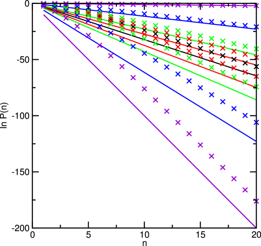
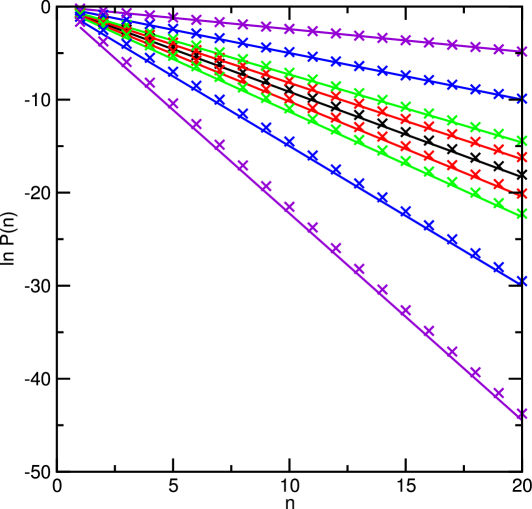
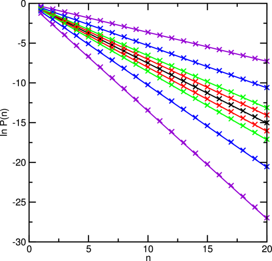
We have numerically evaluated the EFP correlation $P(n)$ for $N=256$ chains for a string of spins starting at site $i=90$ for several values of $T$ and the magnetic field $h$. Figures 2,3,4, and 5 show results for $T=0.1$, 0.5, 1, and 10, respectively.

In all cases it was found that the asymptotic formula (18) describes the numerical data very well. The prefactor $c(T,h)(\geq 1)$ is large at low $T$ and negative values of $h$, as already observed by Shiroishi et al. [6] (compare their Figure 6). For intermediate and high temperatures we observed a very small but seemingly systematic slope when we plotted the difference between the logarithm of the numerical value of $P(n)$ and the expression in the exponent of (18) versus $n$. Due to the smallness of the effect we did not further pursue the origin of this difference, however.

We have also assessed the influence of finite-size and boundary effects on $P(n)$ for $T=0.1$ and $h=\pm 0.99,\pm 0.1$, and 0. For these parameter values we compared the numerical results for $N=256$, starting sites $i=90$ and 91, and $N=512$, $i=240$. No differences beyond the $10^{-7}$ level were found.

In the limit $T\to\infty$ $P(n)=\left(\frac{1}{2}\right)^{n}$ for arbitrary $h$. That is precisely what the $h=0$ results already show at $T=10$ (see Fig. 5). For some selected $h$ and $T$ values we have also compared our values for the decay length of $P(n)$ to those given in Figure 5 of Shiroishi et al. [6]. The results agree.

At low temperature a crossover from the Gaussian $T=0$ behavior (2) at small $n$ to the exponential asymptotics (18) at larger $n$ can be observed, as shown in Fig. 6.

4 Results for the dimerized case

We have calculated $P(n)$ for weak and strong dimerization, $\delta=0.2$ and $\delta=0.8$.

4.1 $\delta=0.2,T=0$

For given dimerization $\delta>0$ there are two critical values for the magnetic field, $h=\pm\delta$. For $|h|<\delta$ the ground state does not depend on $h$. In the Fermion picture it consists of a completely filled lower band and a completely empty upper band. It may thus be expected that correlation functions do not change with $h$ for $h$ within this range.

Figure 7: The EFP correlation $P(n)$ of the dimerized chain as a function of $n^{2}$ for $T=0,\delta=0.2$ and $h=-0.75$, -0.5, -0.25, -0.24, -0.23, -0.22, -0.21, -0.20, +0.201, 0.202, 0.203, 0.204, 0.205, 0.21, 0.25, 0.5, and 0.75 (bottom to top). Heavy lines denote the data for $h=-0.75$, -0.5, -0.25, -0.20 (dashed), +0.205, 0.25, 0.5, and 0.75. On the scale of this figure the data for $h=-0.20,0,$ and +0.20 coincide. Note the rapid variation for $h$ slightly larger than 0.20. (The data for $h=0.202$ and 0.203 coincide on this scale, as do the data for $h=0.204$ and 0.205.)

Figure 8: Gaussian decay parameter $a_{2}$ obtained from the numerical $P(n)$ data shown in Fig. 7.

Figure 9: The EFP correlation $P(n)$ of the dimerized chain for $T=0$, $\delta=0.2$, $h=0.5$ (upper set of curves) and $h=0.2$ (lower set of curves). The strings of sites considered start at site $i=110$ (solid lines) or $i=111$ (dashed lines) of a $N=256$ chain.

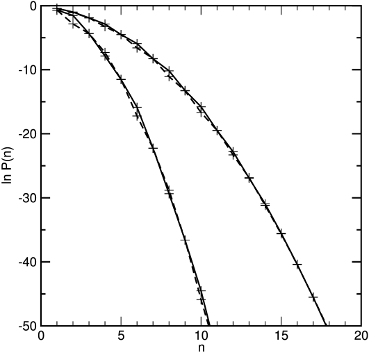
Figure 7 shows $P(n)$ for a large number of $h$ values, with special attention to the critical regions near $h=\pm\delta$. The plot of $\ln P(n)$ vs $n^{2}$ convincingly demonstrates an overall Gaussian behavior, but a closer look at the region $n\leq 10$, for example, reveals some oscillations due to the dimerization. As expected, the EFP correlation does not change as $h$ varies between $-\delta$ and $\delta$.

Figure 8 shows the values of the Gaussian decay parameter $a_{2}$ obtained from the data of Figure 7 by a least-squares fit of the form $\ln P(n)=a_{0}+a_{1}n-a_{2}n^{2}$. The lines between the data points are guides to the eye only. The band-edge singlarity at $h=\delta$ is very prominently visible. In contrast, the behavior near $h=-\delta$, where the lower quasiparticle band approaches complete filling, is less singular.

The changes caused by varying the initial site $i$ are shown in Figure 9 for a sub-critical field $h=0.2$ and a super-critical field $h=0.5$. The solid and dashed lines are for $i=110$ and 111, respectively. The $P(n)$ values for even and odd $i$ seem to coincide for odd string lengths $n$. A closer look at the data shows that at $h=0.2$ this coincidence of data for odd $n$ is indeed perfect. For $h=0.5$ differences at the 1% level show up for all odd $n$. This behavior is not surprising since for odd $n$ the string of $n$ sites contains equal numbers of “weak” and “strong” bonds for both even and odd $i$, hence the EFP as a global quantity of the whole string should be the same, at least in the limit of infinite system size. For even $n$, however, differences are to be expected, and are indeed present in the numerical data. As an extreme example, consider $n=2$: $P(2)$ refers to a single bond and will significantly depend on whether that bond is strong or weak.

In order to assess the effects of system size we have also compared the $N=256$ data to $N=512$ data (for $i=220$ and 221). The data for $h=0.2$ do not depend on $N$, whereas the $h=0.5$ data vary at the percent level between the two $N$ values.

As we are dealing with finite open systems, boundary effects are an issue to be considered. For a given absolute value of the dimerization parameter $|\delta|$ the chain may either start with a “strong” bond or with a “weak” bond. It turns out that switching back and forth between these two possibilities (at $N=256$) is equivalent to switching between even and odd $i$- The equivalence is in fact perfect for subcritical values of $|h|$, for example $h=0$ and 0.2. At $h=\pm 0.5$ we observe , differences at the percent level, the size of which does not change significantly between $N=256$ and $N=512$.

It should be an interesting task to generalize the asymptotic formula (2) to the dimerized case along the lines of [6] in order to better understand the behavior observed in Fig. 8.

4.2 $\delta=0.2,T>0$

Figure 10: The EFP correlation $P(n)$ of the dimerized chain for $T=0.01$, $\delta=0.2$, and $h=1.2$, 1, 0.5, 0.2, 0.1, 0, -0.1, -0.2, -0.5, 1-, -1.2 (top to bottom). Symbols correspond to numerically calculated values, solid lines to the asymptotic formula 18. On the scale of the figure the data for $h=1$ and 1.2 cannot be distinguished.

Figure 11: The EFP correlation $P(n)$ of the dimerized chain for $T=0.03$, $\delta=0.2$, and $h=0.5$, 0, and -0.5 (top to bottom). Symbols correspond to numerically calculated values, solid lines to the asymptotic formula 18.

Figure 12: Similar to Fig. 10, for $T=0.1$

Figure 13: Similar to Fig. 11, for $T=0.3$

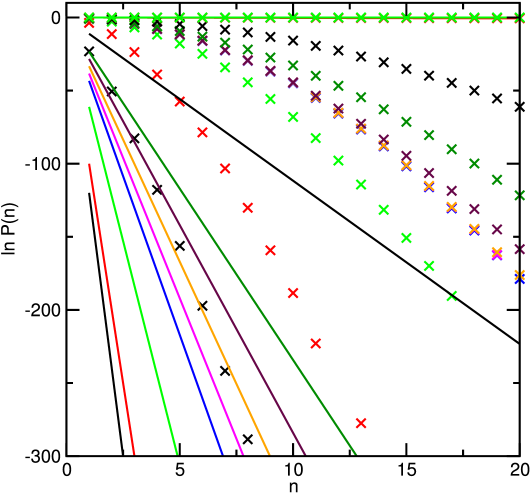
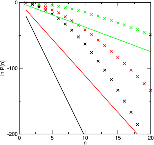
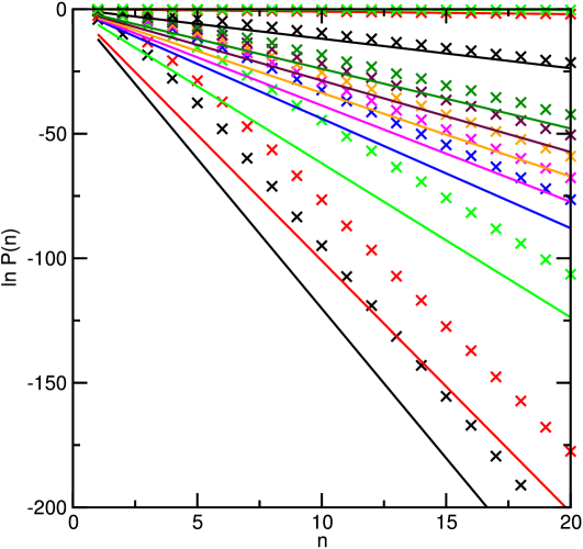
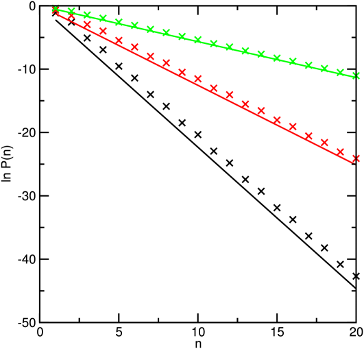
Figure 10 shows data for the low temperature $T=0.01$ and a wide range of $h$ values. The strings of sites considered again start at site $i=110$ of a $N=256$ chain. Comparing the numerically calculated values of $P(n)$ to the asymptotic formula (18) we see clearly that at this low temperature the EFP correlation for $n\leq 20$ still displays the typical Gaussian zero-temperature behavior. The correlations for $h=-0.2$, -0.1, and 0 stay together very closely for $n\leq 20$, whereas those for $h=0.1$ start to deviate for $n>10$ and those for $h=0.2$ even earlier. This is in contrast to $T=0$ (see Fig. 7) where the correlations for all $|h|\leq 0.2$ coincide because the ground state does not change in this $h$ range.

This behavior changes as $T$ increases, as shown in Figures 11 , 12, and 13, for $T=0.03$, 0.1, and 0.3, respectively. Figure 11 shows a crossover of $P(n)$ from Gaussian behavior at small $n$ to exponential behavior at larger $n$. However, at this rather low $T$ value the prefactor $c(T,h)$ in the asymptotic formula (18) is still quite large. Superimposed on the asymptotic behavior the numerical data at $T=0.03$ and $h=0.5$ show the modulation expected due to the alternating exchange couplings. That modulation becomes more visible and the prefactor $c(T,h)$ approaches unity as $T$ grows, see Figs. 12 and 13.

4.3 $\delta=0.8$

Figure 14: The EFP correlation $P(n)$ of the dimerized chain for $T=0$, $\delta=0.8$, and $h=0.99$, 0.9, 0.8, 0, -0.8, -0.9 and -0.99 (top to bottom). The data for $h=0,\pm 0.8$ coincide.

Figure 15: The EFP correlation $P(n)$ of the dimerized chain for $T=0.03$, $\delta=0.8$, and $h=0.99$, 0.9, 0.8, 0, -0.8, -0.9 and -0.99 (top to bottom). Symbols denote numerically calculated values, solid lines show the asymptotic formula (18), with $c(T,h)=1$.

Figure 16: Same data as Figure 15, for $T=0.1$.

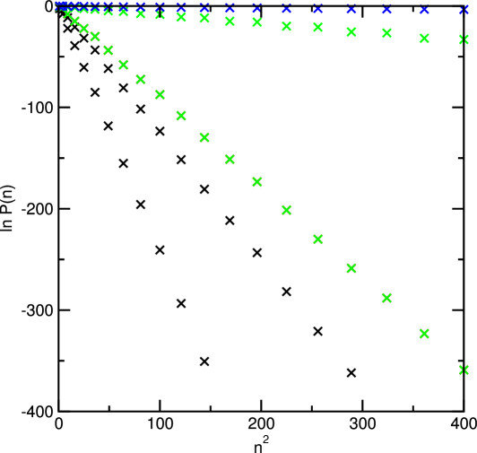
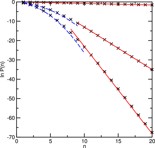
For strong dimerization we present data for $h=\pm 0.99,\pm 0.9,\pm 0.8$, and 0. Figure 14 shows the results for $T=0$. The plot of $\ln P(n)$ as a function of $n^{2}$ shows that the decay is still Gaussian apart from the expected modulation due to the dimerization, which for $\delta=0.8$ is of course expected to be more visible than for $\delta=0.2$. Note that the data points for $h=0,\pm 0.8$ coincide as the ground state stays the same for thes $h$ values.

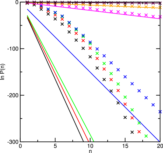
At $T=0.03$ (Figure 15) the data seem to fall naturally into three groups, namely $h<0$, $h=0$, and $h>0$. The $h<0$ data do not seem to reach the proposed asymptotic behavior (18) within the range $n\leq 20$, whereas the other data do so quite nicely. This is not true, however, as closer inspection of the numbers reveals. The data for $h<0$ reach the asymptotics later and with a much larger prefactor $c(T,h)$ in (18).

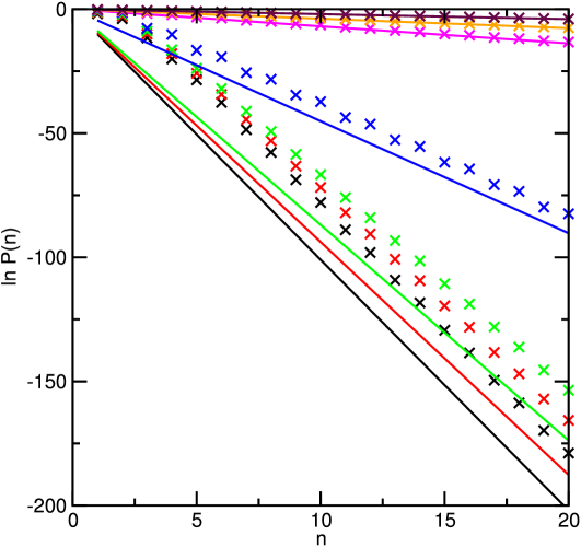
At $T=0.1$ (Figure 16) all $n\geq 5$ data fit to the expected exponential behavior apart from the expected modulation due to dimerization. Note that at this ‘high’ temperature the $h=0$ data stand out alone and the data for the critical field values $h=\pm 0.8$ are much closer to the data for $h=\pm 0.9$ and $\pm 0.99$, in contrast to the situation at $T=0$ (Fig. 14).

5 Concluding Remarks

We have examined the emptiness formation probability (EFP) correlation for homogeneous and dimerized spin-1/2 XX chains numerically by evaluating Pfaffian forms. For the homogeneous XX system the EFP is known to show asymptotically Gaussian behavior in the ground state and exponential behavior at finite temperature. For a homogeneous (anisotropic) XY chain the EFP is known to be exponential at both zero and finite temperatures. The anisotropic XY chain has a gapped single-particle energy spectrum, as does the dimerized XX chain. However, the EFP correlations of the two chains behave differently. Our calculations show that the EFP of the dimerized chain is Gaussian at at zero temperature and exponential at finite temperature. The exponential behavior at finite temperature can be interpreted within a simple free energy picture developed for the homogeneous chain. The generalization of the $T=0$ asymptotic expansion from the homogeneous to the dimerized system is left as a task for future work.

References

- 1. V. E. Korepin, A. G. Izergin, F. Essler, and D. B. Uglov, Phys. Lett. A 190, 182 (1994), preprint cond-mat/9403066.
- 2. F. Essler, H. Frahm, A. Its, and V. Korepin, Nucl. Phys. B 446, 448 (1995), preprint cond-mat/9503142.
- 3. V. E. Korepin, N. M. Bogoliubov, and A. G. Izergin, Quantum Inverse Scattering Method and Correlation Functions (Cambridge University Press, Cambridge, 1993).
- 4. N. Kitanine, J. M. Maillet, N. A. Slavnov, and V. Terras, Nucl. Phys. B 642, 433 (2002), preprint hep-th/0203169.
- 5. N. Kitanine, J. M. Maillet, N. A. Slavnov, and V. Terras, J. Phys. A: Math. Gen. 35, L385 (2002), preprint hep-th/0201134.
- 6. M. Shiroishi, M. Takahashi, and Y. Nishiyama, J. Phys. Soc. Jpn. 70, 3535 (2001), preprint cond-mat/0106062.
- 7. F. Franchini, Ph.D. thesis, SUNY Stony Brook, 2006, preprint arXiv/0801.2734.
- 8. H. E. Boos, V. E. Korepin, Y. Nishiyama, and M. Shiroishi, J. Phys. A: Math. Gen. 35, 4443 (2002), preprint cond-mat/0202346.
- 9. A. G. Abanov and V. E. Korepin, Nucl. Phys. B 647, 565 (2002), preprint cond-mat/0206353.
- 10. H. E. Boos, V. E. Korepin, and F. A. Smirnov, Nucl. Phys. B 658, 417 (2003), preprint hep-th/0209246.
- 11. V. E. Korepin, S. Lukyanov, Y. Nishiyama, and M. Shiroishi, Phys. Lett. A 312, 21 (2002), preprint cond-mat/0210140.
- 12. H. E. Boos and V. E. Korepin, J. Phys. A: Math. Gen. 34, 5311 (2001), preprint hep-th/0104008.
- 13. E. Lieb, T. Schultz, and D. Mattis, Ann. Phys. 16, 407 (1961).
- 14. E. Barouch and B. M. McCoy, Phys. Rev. A 3, 786 (1971).
- 15. A. G. Abanov and F. Franchini, Phys. Lett. A 316, 342 (2003), preprint cond-mat/0307001.
- 16. F. Franchini and A. G. Abanov, J. Phys.. A: Math. Gen. 38, 5069 (2005), preprint cond-mat/0502015.
- 17. J. H. Taylor and G. Müller, Physica 130A, 1 (1985).
- 18. O. Derzhko, T. Krokhmalskii, and J. Stolze, J. Phys. A: Math. Gen. 35, 3573 (2002).
- 19. O. Derzhko, T. Verkholyak, T. Krokhmalskii, and H. Büttner, Phys. Rev. B 73, 214407 (2006).
- 20. S. Katsura, Phys. Rev. 127, 1508 (1962).
- 21. E. B. Fel’dman and M. G. Rudavets, JETP Letters 81, 47 (2005).
- 22. E. I. Kuznetsova and E. B. Fel’dman, JETP 102, 882 (2006).
- 23. T. Garske, Diplom Thesis, Dortmund, 2001.
- 24. J. P. de Lima, T. F. A. Alves, and L. L. Gonçalves, J. Magn. Magn. Materials 298, 95 (2006), preprint cond-mat/0501525.
- 25. W. H. Press, S. A. Teukolsky, W. T. Vetterling, and B. P. Flannery, Numerical Recipes in FORTRAN: the Art of Scientific Computing (Cambridge U.P., Cambridge, 1992).
- 26. M. Gaudin, Nucl. Phys. 15, 89 (1960).
- 27. H. S. Green and C. A. Hurst, Order-Disorder Phenomena (Wiley-Interscience, London, 1964).
- 28. O. Derzhko and T. Krokhmalskii, phys. stat. sol. (b) 208, 221 (1998).
- 29. X. Jia and S. Chakravarty, Phys. Rev. B 74, 172414 (2006).