Experimental Study of the HUM Control Operator for Linear Waves

Gilles Lebeau111Laboratoire J.-A. Dieudonné, Parc Valrose, Nice, France, lebeau@math.unice.fr 222Institut Universitaire de France
Université de Nice
   Maëlle Nodet333Laboratoire J. Kuntzmann, Domaine Universitaire, Grenoble, France, maelle.nodet@inria.fr
Université de Grenoble, INRIA
Abstract

We consider the problem of the numerical approximation of the linear controllability of waves. All our experiments are done in a bounded domain ΩΩ\Omega of the plane, with Dirichlet boundary conditions and internal control. We use a Galerkin approximation of the optimal control operator of the continuous model, based on the spectral theory of the Laplace operator in ΩΩ\Omega. This allows us to obtain surprisingly good illustrations of the main theoretical results available on the controllability of waves, and to formulate some questions for the future analysis of optimal control theory of waves.

1 Introduction

This paper is devoted to the experimental study of the exact controllability of waves. All our experiments will be done in a bounded domain ΩΩ\Omega of the plane, with Dirichlet boundary conditions and with internal control. We use the most natural approach for the numerical computation: a Galerkin approximation of the optimal control operator of the continuous model based on the spectral theory of the Laplace operator in ΩΩ\Omega. This will allow us to obtain surprisingly good illustrations of the main theoretical results available on the controllability of waves, and to formulate some questions for the future analysis of the optimal control theory of waves.

The problem of controllability for linear evolution equations and systems has a long story for which we refer to the review of D.-L. Russel in [Rus78] and to the book of J. L. Lions [Lio88]. Concerning controllability of linear waves, the main theoretical result is the so called “Geometric Control Condition” of C. Bardos, G. Lebeau and J. Rauch [BLR92], GCC in short, which gives a (almost) necessary and sufficient condition for exact controllability. This is a “geometrical optics” condition on the behavior of optical rays inside Ω¯¯Ω\overline{\Omega}. Here, optical rays are just straight lines inside ΩΩ\Omega, reflected at the boundary according to the Snell-Descartes law of reflection. The precise definition of optical rays near points of tangency with the boundary is given in the works of R. Melrose and J. Sjöstrand [MS78] and [MS82]. For internal control, GCC asserts that waves in a regular bounded domain ΩΩ\Omega are exactly controllable by control functions supported in the closure of an open sub-domain U𝑈U and acting during a time T𝑇T, if (and only if, if one allows arbitrary small perturbations of the time control T𝑇T and of the control domain U𝑈U)

GCC: every optical ray of length T𝑇T in ΩΩ\Omega enters the sub-domain U𝑈U.

Even when GCC is satisfied, the numerical computation of the control is not an easy task. The original approach consists first in discretizing the continuous model, and then in computing the control of the discrete system to use it as a numerical approximation of the continuous one. This method has been developed by R. Glowinski et al. (see [GLL90] and [GHL08]), and used for numerical experiments in [AL98]. However, as observed in the first works of R. Glowinski, interaction of waves with a numerical mesh produces spurious high frequency oscillations. In fact, the discrete model is not uniformly exactly controllable when the mesh size goes to zero, since the group velocity converges to zero when the solutions wavelength is comparable to the mesh size. In other words, the processes of numerical discretization and observation or control do not commute. A precise analysis of this lack of commutation and its impact on the computation of the control has been done by E. Zuazua in [Zua02] and [Zua05].

In this paper, we shall use another approach, namely we will discretize the optimal control of the continuous model using a projection of the wave equation onto the finite dimensional space spanned by the eigenfunctions ejsubscript𝑒𝑗e_{j} of the Laplace operator in ΩΩ\Omega with Dirichlet boundary conditions, ej=ωj2ej,ej|Ω=0subscript𝑒𝑗superscriptsubscript𝜔𝑗2subscript𝑒𝑗evaluated-atsubscript𝑒𝑗Ω0-\triangle e_{j}=\omega_{j}^{2}e_{j},e_{j}|_{\partial\Omega=0} , with ωjωsubscript𝜔𝑗𝜔\omega_{j}\leq\omega. Here, ω𝜔\omega will be a cutoff frequency at our disposal. We prove (see lemma 2 in section 2.3) that when GCC is satisfied, our numerical control converges when ω𝜔\omega\rightarrow\infty to the optimal control of the continuous model . Moreover, when GCC is not satisfied, we will do experiments and we will see an exponential blow-up in the cutoff frequency ω𝜔\omega of the norm of the discretized optimal control. These blow-up rates will be compared to theoretical results in section 2.3.

The paper is organized as follows.

Section 2 is devoted to the analysis of the optimal control operator for waves in a bounded regular domain of dsuperscript𝑑\mathbb{R}^{d}. In section 2.1, we recall the definition of the optimal control operator ΛΛ\Lambda. In section 2.2, we recall some known theoretical results on ΛΛ\Lambda: existence, regularity properties and the fact that it preserves the frequency localization. We also state our first conjecture, namely that the optimal control operator ΛΛ\Lambda is a microlocal operator. In section 2.3, we introduce the spectral Galerkin approximation MT,ω1superscriptsubscript𝑀𝑇𝜔1M_{T,\omega}^{-1} of ΛΛ\Lambda, where ω𝜔\omega is a cutoff frequency. We prove the convergence of MT,ω1superscriptsubscript𝑀𝑇𝜔1M_{T,\omega}^{-1} toward ΛΛ\Lambda when ω𝜔\omega\rightarrow\infty, and we analyze the rate of this convergence. We also state our second conjecture on the blow-up rate of MT,ω1superscriptsubscript𝑀𝑇𝜔1M_{T,\omega}^{-1} when GCC is not satisfied. Finally, in section 2.4, we introduce the basis of the energy space in which we compute the matrix of the operator MT,ωsubscript𝑀𝑇𝜔M_{T,\omega}.

Section 3 is devoted to the experimental validation of our Galerkin approximation. In section 3.1 we introduce the 333 different domains of the plane for our experiments: square, disc and trapezoid. In the first two cases, the geodesic flow is totally integrable and the exact eigenfunctions and eigenvalues of the Laplace operator with Dirichlet boundary condition are known. This is not the case for the trapezoid. In section 3.2 we introduce the two different choices of the control operator we use in our experiments. In the first case (non smooth case), we use χ(t,x)=𝟏[0,T]𝟏U𝜒𝑡𝑥subscript10𝑇subscript1𝑈\chi(t,x)={\bf 1}_{[0,T]}{\bf 1}_{U}. In the second case (smooth case), we use a suitable regularization of the first case (see formulas (66) and (67)). Perhaps the main contribution of this paper is to give an experimental evidence that the choice of a smooth enough control operator is the right way to get accuracy on control computing. In section 3.3, in the two cases of the square and the disc, we compare the exact eigenvalues with the eigenvalues computed using the 555-points finite difference approximation of the Laplace operator. In section 3.4, formula (69), we define the reconstruction error of our method. Finally, in section 3.5, in the case of the square geometry, we compare the control function (we choose to reconstruct a single eigenvalue) when the eigenvalues and eigenvectors are computed either with finite differences or with exact formulas, and we study the experimental convergence of our numerical optimal control to the exact optimal control of the continuous model when the cutoff frequency goes to infinity.

The last section, 4, presents various numerical experiments which illustrate the theoretical results of section 2, and are in support of our two conjectures. In section 4.1, our experiments illuminate the fact that the optimal control operator preserves the frequency localization, and that this property is far much stronger when the control function is smooth, as predicted by theoretical results. In section 4.2, we use Dirac and box experiments to illustrate the fact that the optimal control operator shows a behavior very close to the behavior of a pseudo-differential operator: this is in support of our first conjecture. In section 4.3, we plot the reconstruction error as a function of the cutoff frequency: this illuminates how the rate of convergence of the Galerkin approximation depends on the regularity of the control function. In section 4.4, we present various results on the energy of the control function. In section 4.5, we compute the condition number of the matrix MT,ωsubscript𝑀𝑇𝜔M_{T,\omega} for a given control domain U𝑈U, as a function of the control time T𝑇T and the cutoff frequency ω𝜔\omega. In particular, figures 31 and 32 are in support of our second conjecture on the blow-up rate of MT,ω1superscriptsubscript𝑀𝑇𝜔1M_{T,\omega}^{-1} when GCC is not satisfied. In section 4.6, we perform experiments in the disc when GCC is not satisfied, for two different data: in the first case, every optical rays of length T𝑇T starting at a point where the data is not small enters the control domain U𝑈U, and we observe a rather good reconstruction error if the cutoff frequency is not too high. In the second case, there exists an optical ray starting at a point where the data is not small and which never enters the control domain, and we observe a very poor reconstruction at any cutoff frequency. This is a fascinating phenomena which has not been previously studied in theoretical works. It will be of major practical interest to get quantitative results on the best cutoff frequency which optimizes the reconstruction error (this optimal cutoff frequency is equal to \infty when GCC is satisfied, the reconstruction error being equal to 00 in that case), and to estimate the reconstruction error at the optimal cutoff frequency. Clearly, our experiments indicate that a weak Geometric Control Condition associated to the data one wants to reconstruct will enter in such a study.

2 The analysis of the optimal control operator

2.1 The optimal control operator

Here we recall the basic facts we will need in our study of the optimal control operator for linear waves. For more details on the HUM method, we refer to the book of J.-L. Lions [Lio88].

In the framework of the wave equation in a bounded open subset ΩΩ\Omega of dsuperscript𝑑\mathbb{R}^{d} with boundary Dirichlet condition, and for internal control the problem of controllability is stated in the following way. Let T𝑇T be a positive time, U𝑈U a non void open subset of ΩΩ\Omega, and χ(t,x)𝜒𝑡𝑥\chi(t,x) as follows:

χ(t,x)=ψ(t)χ0(x)𝜒𝑡𝑥𝜓𝑡subscript𝜒0𝑥\chi(t,x)=\psi(t)\chi_{0}(x) (1)

where χ0subscript𝜒0\chi_{0} is a real Lsuperscript𝐿L^{\infty} function on Ω¯¯Ω\overline{\Omega}, such that support(χ0)=U¯subscript𝜒0¯𝑈(\chi_{0})=\overline{U} and χ0(x)subscript𝜒0𝑥\chi_{0}(x) is continuous and positive for xU𝑥𝑈x\in U, ψC([0,T])𝜓superscript𝐶0𝑇\psi\in C^{\infty}([0,T]) and ψ(t)>0𝜓𝑡0\psi(t)>0 on ]0,T[.]0,T[. For a given f=(u0,u1)H01(Ω)×L2(Ω),𝑓subscript𝑢0subscript𝑢1superscriptsubscript𝐻01Ωsuperscript𝐿2Ωf=(u_{0},u_{1})\in H_{0}^{1}(\Omega)\times L^{2}(\Omega), the problem is to find a source v(t,x)L2(0,T;L2(Ω))𝑣𝑡𝑥superscript𝐿20𝑇superscript𝐿2Ωv(t,x)\in L^{2}(0,T;L^{2}(\Omega)) such that the solution of the system

{u=χvin ]0,+[×ΩuΩ=0,t>0(u|t=0,tu|t=0)=(0,0)\left\{\begin{array}[c]{c}\square u=\chi v\quad\text{in }]0,+\infty[\times\Omega\\ u_{\mid\partial\Omega}=0,\quad t>0\\ (u|_{t=0},\partial_{t}u|_{t=0})=(0,0)\end{array}\right. (2)

reaches the state f=(u0,u1)𝑓subscript𝑢0subscript𝑢1f=(u_{0},u_{1}) at time T𝑇T. We first rewrite the wave operator in (2) as a first order system. Let A𝐴A be the matrix

iA=(0Id0)𝑖𝐴matrix0𝐼𝑑0iA=\begin{pmatrix}0&Id\\ \triangle&0\end{pmatrix} (3)

Then A𝐴A is a unbounded self-adjoint operator on H=H01(Ω)×L2(Ω)𝐻superscriptsubscript𝐻01Ωsuperscript𝐿2ΩH=H_{0}^{1}(\Omega)\times L^{2}(\Omega), where the scalar product on H01(Ω)superscriptsubscript𝐻01ΩH_{0}^{1}(\Omega) is Ωuv¯dxsubscriptΩ𝑢¯𝑣𝑑𝑥\int_{\Omega}\nabla u\overline{\nabla v}dx and D(A)={u¯=(u0,u1)H,A(u¯)H,u0|Ω=0}D(A)=\{\underline{u}=(u_{0},u_{1})\in H,\ A(\underline{u})\in H,\ u_{0}|_{\partial\Omega}=0\}. Let λ=D𝜆subscript𝐷\lambda=\sqrt{-\triangle_{D}} where Dsubscript𝐷-\triangle_{D} is the canonical isomorphism from H01(Ω)superscriptsubscript𝐻01ΩH_{0}^{1}(\Omega) onto H1(Ω)superscript𝐻1ΩH^{-1}(\Omega). Then λ𝜆\lambda is an isomorphism from H01(Ω)superscriptsubscript𝐻01ΩH_{0}^{1}(\Omega) onto L2(Ω)superscript𝐿2ΩL^{2}(\Omega). The operator B(t)𝐵𝑡B(t) given by

B(t)=(00χ(t,.)λ0)B(t)=\begin{pmatrix}0&0\\ \chi(t,.)\lambda&0\end{pmatrix} (4)

is bounded on H𝐻H, and one has

B(t)=(0λ1χ(t,.)00)B^{*}(t)=\begin{pmatrix}0&\lambda^{-1}\chi(t,.)\\ 0&0\end{pmatrix} (5)

The system (2) is then equivalent to

(tiA)f=B(t)g,f(0)=0formulae-sequencesubscript𝑡𝑖𝐴𝑓𝐵𝑡𝑔𝑓00(\partial_{t}-iA)f=B(t)g,\quad f(0)=0 (6)

with f=(u,tu)𝑓𝑢subscript𝑡𝑢f=(u,\partial_{t}u), g=(λ1v,0)𝑔superscript𝜆1𝑣0g=(\lambda^{-1}v,0). For any g(t)L1([0,[,H)g(t)\in L^{1}([0,\infty[,H), the evolution equation

(tiA)f=B(t)g,f(0)=0formulae-sequencesubscript𝑡𝑖𝐴𝑓𝐵𝑡𝑔𝑓00(\partial_{t}-iA)f=B(t)g,\quad f(0)=0 (7)

admits a unique solution f=S(g)C0([0,+[,H)f=S(g)\in C^{0}([0,+\infty[,H) given by the Duhamel formula

f(t)=0tei(ts)AB(s)g(s)𝑑s𝑓𝑡superscriptsubscript0𝑡superscript𝑒𝑖𝑡𝑠𝐴𝐵𝑠𝑔𝑠differential-d𝑠f(t)=\int_{0}^{t}e^{i(t-s)A}B(s)g(s)ds (8)

Let T>0𝑇0T>0 be given. Let Tsubscript𝑇\mathcal{R}_{T} be the reachable set at time T𝑇T

T={fH,gL2([0,T],H),f=S(g)(T)}subscript𝑇formulae-sequence𝑓𝐻formulae-sequence𝑔superscript𝐿20𝑇𝐻𝑓𝑆𝑔𝑇\mathcal{R}_{T}=\{f\in H,\ \exists g\in L^{2}([0,T],H),\ f=S(g)(T)\} (9)

Then Tsubscript𝑇\mathcal{R}_{T} is a linear subspace of H𝐻H, and is the set of states of the system that one can reach in time T𝑇T, starting from rest, with the action of an L2superscript𝐿2L^{2} source g𝑔g filtered by the control operator B𝐵B. The control problem consists in giving an accurate description of Tsubscript𝑇\mathcal{R}_{T}, and exact controllability is equivalent to the equality T=Hsubscript𝑇𝐻\mathcal{R}_{T}=H. Let us recall some basic facts.

Let =L2([0,T],H)superscript𝐿20𝑇𝐻\mathcal{H}=L^{2}([0,T],H). Let \mathcal{F} be the closed subspace of \mathcal{H} spanned by solutions of the adjoint evolution equation

={h,(tiA)h=0,h(T)=hTH}formulae-sequenceformulae-sequencesubscript𝑡𝑖superscript𝐴0𝑇subscript𝑇𝐻\mathcal{F}=\{h\in\mathcal{H},\ (\partial_{t}-iA^{*})h=0,\ h(T)=h_{T}\in H\} (10)

Observe that, in our context, A=Asuperscript𝐴𝐴A^{*}=A, and the function hh in (10) is given by h(t)=ei(Tt)AhT𝑡superscript𝑒𝑖𝑇𝑡𝐴subscript𝑇h(t)=e^{-i(T-t)A}h_{T}. Let superscript\mathcal{B}^{*} be the adjoint of the operator gS(g)(T)maps-to𝑔𝑆𝑔𝑇g\mapsto S(g)(T). Then superscript\mathcal{B}^{*} is the bounded operator from H𝐻H into \mathcal{H} defined by

(hT)(t)=B(t)ei(Tt)AhTsuperscriptsubscript𝑇𝑡superscript𝐵𝑡superscript𝑒𝑖𝑇𝑡𝐴subscript𝑇\mathcal{B}^{*}(h_{T})(t)=B^{*}(t)e^{-i(T-t)A}h_{T} (11)

For any gL2([0,T],H)𝑔superscript𝐿20𝑇𝐻g\in L^{2}([0,T],H), one has, with fT=S(g)(T)subscript𝑓𝑇𝑆𝑔𝑇f_{T}=S(g)(T) and h(s)=ei(Ts)AhT𝑠superscript𝑒𝑖𝑇𝑠𝐴subscript𝑇h(s)=e^{-i(T-s)A}h_{T} the fundamental identity

(fT|hT)H=0T(B(s)g(s)|h(s))𝑑s=(g|(hT))subscriptconditionalsubscript𝑓𝑇subscript𝑇𝐻superscriptsubscript0𝑇conditional𝐵𝑠𝑔𝑠𝑠differential-d𝑠subscriptconditional𝑔superscriptsubscript𝑇(f_{T}|h_{T})_{H}=\int_{0}^{T}(B(s)g(s)|h(s))ds=(g|\mathcal{B}^{*}(h_{T}))_{\mathcal{H}} (12)

From (12), one gets easily that the following holds true

Tis a dense subspace of His an injective operatorsubscript𝑇is a dense subspace of 𝐻superscriptis an injective operator\mathcal{R}_{T}\ \text{is a dense subspace of }\ H\ \Longleftrightarrow\ \mathcal{B}^{*}\ \text{is an injective operator} (13)

which shows that approximate controllability is equivalent to a uniqueness result on the adjoint equation. Moreover, one gets from (12), using the Riesz and closed graph theorems, that the following holds true

T=HC,hChhH\mathcal{R}_{T}=H\quad\quad\Longleftrightarrow\ \exists C,\quad\|h\|\leq C\|\mathcal{B}^{*}h\|\quad\forall h\in H (14)

This is an observability inequality, and superscript\mathcal{B}^{*} is called the observability operator. We rewrite the observability inequality (14) in a more explicit form

C,hH2C0TB(s)ei(Ts)AhH2𝑑shHformulae-sequence𝐶subscriptsuperscriptnorm2𝐻𝐶superscriptsubscript0𝑇superscriptsubscriptnormsuperscript𝐵𝑠superscript𝑒𝑖𝑇𝑠𝐴𝐻2differential-d𝑠for-all𝐻\exists C,\quad\|h\|^{2}_{H}\leq C\int_{0}^{T}\|B^{*}(s)e^{-i(T-s)A}h\|_{H}^{2}ds\quad\forall h\in H (15)

Assuming that (15) holds true, then T=Hsubscript𝑇𝐻\mathcal{R}_{T}=H, Im()Imsuperscript\textrm{Im}(\mathcal{B}^{*}) is a closed subspace of \mathcal{H}, and superscript\mathcal{B}^{*} is an isomorphism of H𝐻H onto Im()Imsuperscript\textrm{Im}(\mathcal{B}^{*}). For any fH𝑓𝐻f\in H, let 𝒞fsubscript𝒞𝑓\mathcal{C}_{f} be the set of control functions g𝑔g driving 00 to f𝑓f in time T𝑇T

𝒞f={gL2([0,T],H),f=0Tei(Ts)AB(s)g(s)𝑑s}subscript𝒞𝑓formulae-sequence𝑔superscript𝐿20𝑇𝐻𝑓superscriptsubscript0𝑇superscript𝑒𝑖𝑇𝑠𝐴𝐵𝑠𝑔𝑠differential-d𝑠\mathcal{C}_{f}=\left\{g\in L^{2}([0,T],H),\quad f=\int_{0}^{T}e^{i(T-s)A}B(s)g(s)ds\right\} (16)

From (12), one gets

𝒞f=g0+(Im),g0Im𝒞fformulae-sequencesubscript𝒞𝑓subscript𝑔0superscriptImsuperscriptperpendicular-tosubscript𝑔0Imsuperscriptsubscript𝒞𝑓\mathcal{C}_{f}=g_{0}+(\textrm{Im}\mathcal{B}^{*})^{\perp},\quad g_{0}\in\textrm{Im}\mathcal{B}^{*}\cap\mathcal{C}_{f} (17)

and g0=hTsubscript𝑔0superscriptsubscript𝑇g_{0}=\mathcal{B}^{*}h_{T} is the optimal control in the sense that

min{gL2([0,T],H),g𝒞f}is achieved atg=g0subscriptnorm𝑔superscript𝐿20𝑇𝐻𝑔subscript𝒞𝑓is achieved at𝑔subscript𝑔0\min\{\|g\|_{L^{2}([0,T],H)},\ g\in\mathcal{C}_{f}\}\quad\text{is achieved at}\ g=g_{0} (18)

Let Λ:HH,Λ(f)=hT:Λformulae-sequence𝐻𝐻Λ𝑓subscript𝑇\Lambda:H\rightarrow H,\ \Lambda(f)=h_{T} be the control map, so that the optimal control g0subscript𝑔0g_{0} is equal to g0(t)=B(t)ei(Tt)AΛ(f)subscript𝑔0𝑡superscript𝐵𝑡superscript𝑒𝑖𝑇𝑡𝐴Λ𝑓g_{0}(t)=B^{*}(t)e^{-i(T-t)A}\Lambda(f). Then ΛΛ\Lambda is exactly the inverse of the map MT:HH:subscript𝑀𝑇𝐻𝐻M_{T}:H\rightarrow H with

MT=0Tm(Tt)𝑑t=0Tm(s)𝑑sm(s)=eisAB(Ts)B(Ts)eisAsubscript𝑀𝑇superscriptsubscript0𝑇𝑚𝑇𝑡differential-d𝑡superscriptsubscript0𝑇𝑚𝑠differential-d𝑠𝑚𝑠superscript𝑒𝑖𝑠𝐴𝐵𝑇𝑠superscript𝐵𝑇𝑠superscript𝑒𝑖𝑠superscript𝐴\begin{array}[]{rcl}M_{T}&=&\displaystyle\int_{0}^{T}m(T-t)dt=\int_{0}^{T}m(s)ds\vskip 6.0pt plus 2.0pt minus 2.0pt\\ m(s)&=&e^{isA}B(T-s)B^{*}(T-s)e^{-isA^{*}}\end{array} (19)

Observe that m(s)=m(s)𝑚𝑠superscript𝑚𝑠m(s)=m^{*}(s) is a bounded, self-adjoint, non-negative operator on H𝐻H. Exact controllability is thus equivalent to

C>0,MT=0Tei(Tt)A(000χ2(t,.))ei(Tt)A𝑑tCId\exists C>0,\quad M_{T}=\int_{0}^{T}e^{i(T-t)A}\begin{pmatrix}0&0\\ 0&\chi^{2}(t,.)\end{pmatrix}e^{-i(T-t)A}dt\geq CId (20)

With Λ=MT1Λsuperscriptsubscript𝑀𝑇1\Lambda=M_{T}^{-1}, the optimal control is then given by g0(t)=B(t)ei(Tt)AΛ(f)subscript𝑔0𝑡superscript𝐵𝑡superscript𝑒𝑖𝑇𝑡𝐴Λ𝑓g_{0}(t)=B^{*}(t)e^{-i(T-t)A}\Lambda(f) and is by (5) of the form g0=(λ1χtw,0)subscript𝑔0superscript𝜆1𝜒subscript𝑡𝑤0g_{0}=(\lambda^{-1}\chi\partial_{t}w,0) where w(t)=ei(Tt)AΛ(f)𝑤𝑡superscript𝑒𝑖𝑇𝑡𝐴Λ𝑓w(t)=e^{-i(T-t)A}\Lambda(f) is the solution of

{w=0in ×Ω,wΩ=0(w(T,.),tw(T,.))=Λ(f)\left\{\begin{array}[c]{c}\square w=0\quad\text{in }\mathbb{R}\times\Omega,\quad w_{\mid\partial\Omega}=0\\ (w(T,.),\partial_{t}w(T,.))=\Lambda(f)\end{array}\right. (21)

Thus, the optimal control function v𝑣v in (2) is equal to v=χtw𝑣𝜒subscript𝑡𝑤v=\chi\partial_{t}w, where w𝑤w is the solution of the dual problem (21). The operator Λ=MT1Λsuperscriptsubscript𝑀𝑇1\Lambda=M_{T}^{-1}, with MTsubscript𝑀𝑇M_{T} given by (20) is called the optimal control operator.

2.2 Theoretical results

In this section we recall some theoretical results on the analysis of the optimal control operator ΛΛ\Lambda. We will assume here that ΩΩ\Omega is a bounded open subset of dsuperscript𝑑\mathbb{R}^{d} with smooth boundary ΩΩ\partial\Omega, and that any straight line in dsuperscript𝑑\mathbb{R}^{d} has only finite order of contacts with the boundary. In that case, optical rays are uniquely defined. See an example of such rays in figure 1.
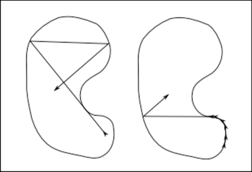
Refer to caption
Figure 1: Example of optical rays.

Let M=Ω×t𝑀Ωsubscript𝑡M=\Omega\times\mathbb{R}_{t}. The phase space is

TbM=TM¯TMTMTM.superscriptsuperscript𝑇𝑏𝑀superscript𝑇¯𝑀subscriptsuperscript𝑇𝑀similar-to-or-equalssuperscript𝑇𝑀superscript𝑇𝑀{}^{b}T^{*}M=T^{*}\overline{M}\setminus T^{*}_{\partial M}\simeq T^{*}M\cup T^{*}\partial M.

The characteristic variety of the wave operator is the closed subset ΣΣ\Sigma of TbMsuperscriptsuperscript𝑇𝑏𝑀{}^{b}T^{*}M of points (x,t,ξ,τ)𝑥𝑡𝜉𝜏(x,t,\xi,\tau) such that |τ|=|ξ|𝜏𝜉|\tau|=|\xi| when xΩ𝑥Ωx\in\Omega and |τ||ξ|𝜏𝜉|\tau|\geq|\xi| when xΩ𝑥Ωx\in\partial\Omega. Let SbΩ¯superscriptsuperscript𝑆𝑏¯Ω{}^{b}S^{*}\overline{\Omega} be the set of points

SbΩ¯={(x0,ξ0), with |ξ0|=1 if x0Ω,|ξ0|1 if x0Ω}{}^{b}S^{*}\overline{\Omega}=\{(x_{0},\xi_{0}),\textrm{ with }|\xi_{0}|=1\textrm{ if }x_{0}\in\Omega,|\xi_{0}|\leq 1\textrm{ if }x_{0}\in\partial\Omega\}

For ρ0=(x0,ξ0)SbΩ¯subscript𝜌0subscript𝑥0subscript𝜉0superscriptsuperscript𝑆𝑏¯Ω\rho_{0}=(x_{0},\xi_{0})\in{{}^{b}S}^{*}\overline{\Omega}, and τ=±1𝜏plus-or-minus1\tau=\pm 1, we shall denote by s(γρ0(s),tsτ,τ),sformulae-sequence𝑠subscript𝛾subscript𝜌0𝑠𝑡𝑠𝜏𝜏𝑠s\rightarrow(\gamma_{\rho_{0}}(s),t-s\tau,\tau),s\in\mathbb{R} the generalized bicharacteristic ray of the wave operator, issued from (x0,ξ0,t,τ)subscript𝑥0subscript𝜉0𝑡𝜏(x_{0},\xi_{0},t,\tau). For the construction of the Melrose-Sjöstrand flow, we refer to [MS78], [MS82] and to [Hör85], vol 3, chapter XXIV . Then sγρ0(s)=(x(ρ0,s),ξ(ρ0,s))𝑠subscript𝛾subscript𝜌0𝑠𝑥subscript𝜌0𝑠𝜉subscript𝜌0𝑠s\rightarrow\gamma_{\rho_{0}}(s)=(x(\rho_{0},s),\xi(\rho_{0},s)) is the optical ray starting at x0subscript𝑥0x_{0} in the direction ξ0subscript𝜉0\xi_{0}. When x0Ωsubscript𝑥0Ωx_{0}\in\partial\Omega and |ξ0|<1subscript𝜉01|\xi_{0}|<1, then the right (respectively left) derivative of x(ρ0,s)𝑥subscript𝜌0𝑠x(\rho_{0},s) at s=0𝑠0s=0 is equal to the unit vector in dsuperscript𝑑\mathbb{R}^{d} which projects on ξ0TΩsubscript𝜉0superscript𝑇Ω\xi_{0}\in T^{*}\partial\Omega and which points inside (respectively outside) ΩΩ\Omega. In all other cases, x(ρ0,s)𝑥subscript𝜌0𝑠x(\rho_{0},s) is derivable at s=0𝑠0s=0 with derivative equal to ξ0subscript𝜉0\xi_{0}.

We first recall the theorem of [BLR92], which gives the existence of the operator ΛΛ\Lambda:

Theorem 1

If the geometric control condition GCC holds true, then MTsubscript𝑀𝑇M_{T} is an isomorphism.

Next, we recall some new theoretical results obtained in [DL09]. For these results, the choice of the control function χ(t,x)𝜒𝑡𝑥\chi(t,x) in (1) will be essential.

Definition 1

The control function χ(t,x)=ψ(t)χ0(x)𝜒𝑡𝑥𝜓𝑡subscript𝜒0𝑥\chi(t,x)=\psi(t)\chi_{0}(x) is smooth if χ0C(Ω¯)subscript𝜒0superscript𝐶¯Ω\chi_{0}\in C^{\infty}(\overline{\Omega}) and ψ(t)𝜓𝑡\psi(t) is flat at t=0𝑡0t=0 and t=T𝑡𝑇t=T.

For s𝑠s\in\mathbb{R}, we denote by Hs(Ω,)superscript𝐻𝑠ΩH^{s}(\Omega,\triangle) the domain of the operator (Dirichlet)s/2superscriptsubscriptDirichlet𝑠2(-\triangle_{\text{Dirichlet}})^{s/2}. One has H0(Ω,)=L2(Ω)superscript𝐻0Ωsuperscript𝐿2ΩH^{0}(\Omega,\triangle)=L^{2}(\Omega), H1(Ω,)=H01(Ω)superscript𝐻1Ωsuperscriptsubscript𝐻01ΩH^{1}(\Omega,\triangle)=H_{0}^{1}(\Omega), and if (ej)j1subscriptsubscript𝑒𝑗𝑗1(e_{j})_{j\geq 1} is an L2superscript𝐿2L^{2} orthonormal basis of eigenfunctions of -\triangle with Dirichlet boundary conditions, ej=ωj2ejsubscript𝑒𝑗superscriptsubscript𝜔𝑗2subscript𝑒𝑗-\triangle e_{j}=\omega_{j}^{2}e_{j}, 0<ω1ω20subscript𝜔1subscript𝜔20<\omega_{1}\leq\omega_{2}\leq..., one has

Hs(Ω,)={f𝒟(Ω),f=jfjej,jωj2s|fj|2<}superscript𝐻𝑠Ωformulae-sequence𝑓superscript𝒟Ωformulae-sequence𝑓subscript𝑗subscript𝑓𝑗subscript𝑒𝑗subscript𝑗superscriptsubscript𝜔𝑗2𝑠superscriptsubscript𝑓𝑗2H^{s}(\Omega,\triangle)=\{f\in\mathcal{D}^{\prime}(\Omega),f=\sum_{j}f_{j}e_{j},\ \sum_{j}\omega_{j}^{2s}|f_{j}|^{2}<\infty\} (22)

The following result of [DL09] says that, under the hypothesis that the control function χ(t,x)𝜒𝑡𝑥\chi(t,x) is smooth, the optimal control operator ΛΛ\Lambda preserves the regularity:

Theorem 2

Assume that the geometric control condition GCC holds true, and that the control function χ(t,x)𝜒𝑡𝑥\chi(t,x) is smooth. Then the optimal control operator ΛΛ\Lambda is an isomorphism of Hs+1(Ω,Δ)Hs(Ω,Δ)direct-sumsuperscript𝐻𝑠1ΩΔsuperscript𝐻𝑠ΩΔH^{s+1}(\Omega,\Delta)\oplus H^{s}(\Omega,\Delta) for all s0𝑠0s\geq 0.

Observe that theorem 1 is a particular case of theorem 2 with s=0𝑠0s=0. In our experimental study, we will see in section 4.3 that the regularity of the control function χ(t,x)𝜒𝑡𝑥\chi(t,x) is not only a nice hypothesis to get theoretical results. It is also very efficient to get accuracy in the numerical computation of the control function. In other words, the usual choice of the control function χ(t,x)=𝟏[0,T]𝟏U𝜒𝑡𝑥subscript10𝑇subscript1𝑈\chi(t,x)={\bf 1}_{[0,T]}{\bf 1}_{U} is a very poor idea to compute a control.

The next result says that the optimal control operator ΛΛ\Lambda preserves the frequency localization. To state this result we briefly introduce the material needed for the Littlewood-Paley decomposition. Let ϕitalic-ϕ\phi \in C([0,[),C^{\infty}([0,\infty[), with ϕ(x)=1italic-ϕ𝑥1\phi(x)=1 for |x|1/2𝑥12|x|\leq 1/2 and ϕ(x)=0italic-ϕ𝑥0\phi(x)=0 for |x|1𝑥1|x|\geq 1. Set ψ(x)=ϕ(x)ϕ(2x)𝜓𝑥italic-ϕ𝑥italic-ϕ2𝑥\psi(x)=\phi(x)-\phi(2x). Then ψC0()𝜓superscriptsubscript𝐶0superscript\psi\in C_{0}^{\infty}(\mathbb{R}^{\ast}), ψ𝜓\psi vanishes outside [1/4,1]141[1/4,1], and one has

ϕ(s)+k=1ψ(2ks)=1,s[0,[\phi(s)+\sum_{k=1}^{\infty}\psi(2^{-k}s)=1,\qquad\quad\forall s\in[0,\infty[

Set ψ0(s)=ϕ(s)subscript𝜓0𝑠italic-ϕ𝑠\psi_{0}(s)=\phi(s) and ψk(s)=ψ(2ks)subscript𝜓𝑘𝑠𝜓superscript2𝑘𝑠\psi_{k}(s)=\psi(2^{-k}s) for k1𝑘1k\geq 1. We then define the spectral localization operators ψk(D),subscript𝜓𝑘𝐷\psi_{k}(D), k,𝑘k\in\mathbb{N}, in the following way: for u=jajej,𝑢subscript𝑗subscript𝑎𝑗subscript𝑒𝑗u=\sum_{j}a_{j}e_{j}, we define

ψk(D)u=jψk(ωj)ajejsubscript𝜓𝑘𝐷𝑢subscript𝑗subscript𝜓𝑘subscript𝜔𝑗subscript𝑎𝑗subscript𝑒𝑗\psi_{k}(D)u=\sum_{j}\psi_{k}(\omega_{j})a_{j}e_{j} (23)

One has kψk(D)=Idsubscript𝑘subscript𝜓𝑘𝐷𝐼𝑑\sum_{k}\psi_{k}(D)=Id and ψi(D)ψj(D)=0subscript𝜓𝑖𝐷subscript𝜓𝑗𝐷0\psi_{i}(D)\psi_{j}(D)=0 for |ij|2𝑖𝑗2|i-j|\geq 2. In addition, we introduce

Sk(D)=j=0kψj(D)=ψ0(2kD),k0formulae-sequencesubscript𝑆𝑘𝐷superscriptsubscript𝑗0𝑘subscript𝜓𝑗𝐷subscript𝜓0superscript2𝑘𝐷𝑘0S_{k}(D)=\sum_{j=0}^{k}\psi_{j}(D)=\psi_{0}(2^{-k}D),\qquad\quad k\geq 0 (24)

Obviously, the operators ψk(D)subscript𝜓𝑘𝐷\psi_{k}(D) and Sk(D)subscript𝑆𝑘𝐷S_{k}(D) acts as bounded operators on H=H01×L2𝐻subscriptsuperscript𝐻10superscript𝐿2H=H^{1}_{0}\times L^{2}. The spectral localization result of [DL09] reads as follows.

Theorem 3

Assume that the geometric control condition GCC holds true, and that the control function χ(t,x)𝜒𝑡𝑥\chi(t,x) is smooth. There exists C>0𝐶0C>0 such that for every k𝑘k\in\mathbb{N}, the following inequality holds true

ψk(D)ΛΛψk(D)HC2kSk(D)ΛΛSk(D)HC2kmissing-subexpressionsubscriptnormsubscript𝜓𝑘𝐷ΛΛsubscript𝜓𝑘𝐷𝐻𝐶superscript2𝑘missing-subexpressionmissing-subexpressionsubscriptnormsubscript𝑆𝑘𝐷ΛΛsubscript𝑆𝑘𝐷𝐻𝐶superscript2𝑘missing-subexpression\begin{array}[]{rcl}&\|\psi_{k}(D)\Lambda-\Lambda\psi_{k}(D)\|_{H}\leq C2^{-k}\\ &\|S_{k}(D)\Lambda-\Lambda S_{k}(D)\|_{H}\leq C2^{-k}\\ \end{array} (25)

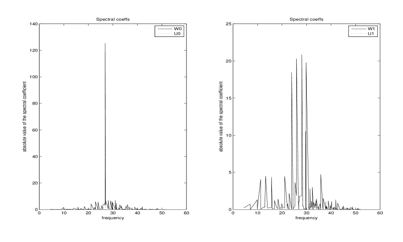
Theorem 3 states that the optimal control operator ΛΛ\Lambda, up to lower order terms, acts individually on each frequency block of the solution. For instance, if ensubscript𝑒𝑛e_{n} is the n𝑛n-th eigenvector of the orthonormal basis of L2(Ω),superscript𝐿2ΩL^{2}(\Omega), if one drives the data (0,0)00(0,0) to (en,0)subscript𝑒𝑛0(e_{n},0) in (2) using the optimal control, both the solution u𝑢u and control v𝑣v in equation (2) will essentially live at frequency ωnsubscript𝜔𝑛\omega_{n} for n𝑛n large. We shall do experiments on this fact in section 4.1, and we will clearly see the impact of the regularity of the control function χ(t,x)𝜒𝑡𝑥\chi(t,x) on the accuracy of the frequency localization of the numerical control.

Since by the above results the optimal control operator ΛΛ\Lambda preserves the regularity and the frequency localization, it is very natural to expect that ΛΛ\Lambda is in fact a micro-local operator, and in particular preserves the wave front set. For an introduction to micro-local analysis and pseudo-differential calculus, we refer to [Tay81] and [Hör85]. In [DL09], it is proved that the optimal control operator ΛΛ\Lambda for waves on a compact Riemannian manifold without boundary is in fact an elliptic 2×2222\times 2 matrix of pseudo-differential operators. This is quite an easy result, since if χ(t,x)𝜒𝑡𝑥\chi(t,x) is smooth the Egorov theorem implies that the operator MTsubscript𝑀𝑇M_{T} given by (20) is a 2×2222\times 2 matrix of pseudo-differential operators. Moreover, the geometric control condition GCC implies easily that MTsubscript𝑀𝑇M_{T} is elliptic. Since MTsubscript𝑀𝑇M_{T} is self adjoint, the fact that MTsubscript𝑀𝑇M_{T} is an isomorphism follows then from Ker(MT)={0}𝐾𝑒𝑟subscript𝑀𝑇0Ker(M_{T})=\{0\}, which is equivalent to the injectivity of superscript\mathcal{B}^{*}. This is proved in [BLR92] as a consequence of the uniqueness theorem of Calderon for the elliptic second order operator \triangle. Then it follows that its inverse Λ=MT1Λsuperscriptsubscript𝑀𝑇1\Lambda=M_{T}^{-1} is an elliptic pseudo-differential operator.

In our context, for waves in a bounded regular open subset ΩΩ\Omega of dsuperscript𝑑\mathbb{R}^{d} with boundary Dirichlet condition, the situation is far much complicated, since there is no Egorov theorem in the geometric setting of a manifold with boundary. In fact, the Melrose-Sjöstrand theorem [MS78], [MS82] on propagation of singularities at the boundary (see also [Hör85], vol 3, chapter XXIV for a proof) implies that the operator MTsubscript𝑀𝑇M_{T} given by (20) is a microlocal operator, but this is not sufficient to imply that its inverse ΛΛ\Lambda is micro-local. However let ρ0=(x0,ξ0)TΩ,|ξ0|=1formulae-sequencesubscript𝜌0subscript𝑥0subscript𝜉0superscript𝑇Ωsubscript𝜉01\rho_{0}=(x_{0},\xi_{0})\in T^{*}\Omega,|\xi_{0}|=1 be a point in the cotangent space such that the two optical rays defined by the Melrose-Sjöstrand flow (see [MS78], [MS82]) s[0,T]γ±ρ0(s)=(x(±ρ0,s),ξ(±ρ0,s))𝑠0𝑇subscript𝛾plus-or-minussubscript𝜌0𝑠𝑥plus-or-minussubscript𝜌0𝑠𝜉plus-or-minussubscript𝜌0𝑠s\in[0,T]\rightarrow\gamma_{\pm\rho_{0}}(s)=(x(\pm\rho_{0},s),\xi(\pm\rho_{0},s)), with ±ρ0=(x0,±ξ0)plus-or-minussubscript𝜌0subscript𝑥0plus-or-minussubscript𝜉0\pm\rho_{0}=(x_{0},\pm\xi_{0}), starting at x0subscript𝑥0x_{0} in the directions ±ξ0plus-or-minussubscript𝜉0\pm\xi_{0} have only transversal intersections with the boundary. Then it is not hard to show using formula (20) and the parametrix of the wave operator, inside ΩΩ\Omega and near transversal reflection points at the boundary ΩΩ\partial\Omega, as presented in figure 2, that MTsubscript𝑀𝑇M_{T} is microlocally at ρ0subscript𝜌0\rho_{0} an elliptic 2×2222\times 2 matrix of elliptic pseudo-differential operators.
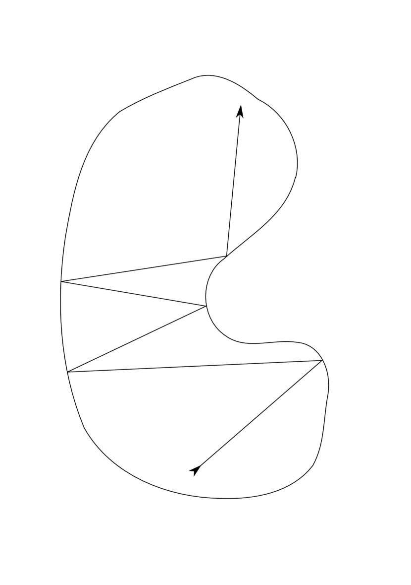
Refer to caption
Figure 2: Example of optical ray with only transversal reflection points.

More precisely, let J𝐽J be the isomorphism from H01L2direct-sumsubscriptsuperscript𝐻10superscript𝐿2H^{1}_{0}\oplus L^{2} on L2L2direct-sumsuperscript𝐿2superscript𝐿2L^{2}\oplus L^{2} given by

J=12(λiλi)𝐽12𝜆𝑖𝜆𝑖J={1\over 2}\left(\begin{array}[c]{cc}\lambda&-i\\ \lambda&i\end{array}\right) (26)

One has 2Ju¯L2L22=u¯H01L222subscriptsuperscriptnorm𝐽¯𝑢2direct-sumsuperscript𝐿2superscript𝐿2subscriptsuperscriptnorm¯𝑢2direct-sumsubscriptsuperscript𝐻10superscript𝐿22\|J\underline{u}\|^{2}_{L^{2}\oplus L^{2}}=\|\underline{u}\|^{2}_{H^{1}_{0}\oplus L^{2}}, and if u(t,x)𝑢𝑡𝑥u(t,x) is the solution of the wave operator u=0𝑢0\Box u=0 with Dirichlet boundary conditions on ΩΩ\partial\Omega, and Cauchy data at time t0subscript𝑡0t_{0} equal to (u0,u1)subscript𝑢0subscript𝑢1(u_{0},u_{1}), then one has

λu(t,.)=λcos((tt0)λ)u0+sin((tt0)λ)u1=ei(tt0)λ(λu0iu12)+ei(tt0)λ(λu0+iu12)\begin{array}[]{rcl}\lambda u(t,.)=&\lambda\cos((t-t_{0})\lambda)u_{0}+\sin((t-t_{0})\lambda)u_{1}\\ =&e^{i(t-t_{0})\lambda}\Big{(}{\lambda u_{0}-iu_{1}\over 2}\Big{)}+e^{-i(t-t_{0})\lambda}\Big{(}{\lambda u_{0}+iu_{1}\over 2}\Big{)}\end{array} (27)

so the effect of the isomorphism J𝐽J is to split the solution u(t,x)𝑢𝑡𝑥u(t,x) into a sum of two waves with positive and negative temporal frequency. Moreover, one has

JeitAJ1=(eitλ00eitλ)𝐽superscript𝑒𝑖𝑡𝐴superscript𝐽1superscript𝑒𝑖𝑡𝜆00superscript𝑒𝑖𝑡𝜆Je^{itA}J^{-1}=\left(\begin{array}[c]{cc}e^{it\lambda}&0\\ 0&e^{-it\lambda}\end{array}\right) (28)

Then JMTJ1𝐽subscript𝑀𝑇superscript𝐽1JM_{T}J^{-1} acts as a non negative self-adjoint operator on L2L2direct-sumsuperscript𝐿2superscript𝐿2L^{2}\oplus L^{2}, and is equal to

JMTJ1=12(Q+𝒯𝒯Q)Q±=0Te±isλχ2(Ts,.)eisλds𝒯=0Teisλχ2(Ts,.)eisλds\begin{array}[]{rcl}JM_{T}J^{-1}=&{1\over 2}\left(\begin{array}[c]{cc}Q_{+}&-\mathcal{T}\\ -\mathcal{T}^{*}&Q_{-}\end{array}\right)\\ Q_{\pm}=&\int_{0}^{T}e^{\pm is\lambda}\chi^{2}(T-s,.)e^{\mp is\lambda}ds\\ \mathcal{T}=&\int_{0}^{T}e^{is\lambda}\chi^{2}(T-s,.)e^{is\lambda}ds\end{array} (29)

From (29), using the parametrix of the wave operator, inside ΩΩ\Omega and near transversal reflection points at the boundary ΩΩ\partial\Omega, and integration by parts to show that 𝒯𝒯\mathcal{T} is a smoothing operator, it is not difficult to get that JMTJ1𝐽subscript𝑀𝑇superscript𝐽1JM_{T}J^{-1} is microlocally at ρ0TΩsubscript𝜌0superscript𝑇Ω\rho_{0}\in T^{*}\Omega a pseudo-differential operator of order zero with principal symbol

σ0(JMTJ1)(ρ0)=12(q+(x0,ξ0)00q(x0,ξ0))q±(x0,ξ0)=0Tχ2(Ts,x(±ρ0,s))𝑑smissing-subexpressionsubscript𝜎0𝐽subscript𝑀𝑇superscript𝐽1subscript𝜌012subscript𝑞subscript𝑥0subscript𝜉000subscript𝑞subscript𝑥0subscript𝜉0missing-subexpressionmissing-subexpressionsubscript𝑞plus-or-minussubscript𝑥0subscript𝜉0superscriptsubscript0𝑇superscript𝜒2𝑇𝑠𝑥plus-or-minussubscript𝜌0𝑠differential-d𝑠missing-subexpression\begin{array}[]{rcl}&\sigma_{0}(JM_{T}J^{-1})(\rho_{0})={1\over 2}\left(\begin{array}[c]{cc}q_{+}(x_{0},\xi_{0})&0\\ 0&q_{-}(x_{0},\xi_{0})\end{array}\right)\\ &q_{\pm}(x_{0},\xi_{0})=\int_{0}^{T}\chi^{2}(T-s,x(\pm\rho_{0},s))ds\end{array} (30)

Obviously, condition (GCC) guarantees that σ0(JMTJ1)(ρ0)subscript𝜎0𝐽subscript𝑀𝑇superscript𝐽1subscript𝜌0\sigma_{0}(JM_{T}J^{-1})(\rho_{0}) is elliptic, and therefore JΛJ1𝐽Λsuperscript𝐽1J\Lambda J^{-1} will be at ρ0subscript𝜌0\rho_{0} a pseudo-differential operator of order zero with principal symbol

σ0(JΛJ1)(ρ0)=2(q+1(x0,ξ0)00q1(x0,ξ0))subscript𝜎0𝐽Λsuperscript𝐽1subscript𝜌02superscriptsubscript𝑞1subscript𝑥0subscript𝜉000superscriptsubscript𝑞1subscript𝑥0subscript𝜉0\sigma_{0}(J\Lambda J^{-1})(\rho_{0})=2\left(\begin{array}[c]{cc}q_{+}^{-1}(x_{0},\xi_{0})&0\\ 0&q_{-}^{-1}(x_{0},\xi_{0})\end{array}\right) (31)

Therefore, the only difficulty in order to prove that ΛΛ\Lambda is a microlocal operator is to get a precise analysis of the structure of the operator MTsubscript𝑀𝑇M_{T} near rays which are tangent to the boundary. Since the set of ρbSΩ¯superscript𝑏𝜌superscript𝑆¯Ω\rho\in^{b}S^{*}\overline{\Omega} for which the optical ray γρ(s)subscript𝛾𝜌𝑠\gamma_{\rho}(s) has only transversal points of intersection with the boundary is dense in TΩ¯TΩsuperscript𝑇¯Ωsubscriptsuperscript𝑇ΩT^{*}\overline{\Omega}\setminus T^{*}_{\partial\Omega} (see [Hör85]), it is not surprising that our numerical experiments in section 4.2 (where we compute the optimal control associated to a Dirac mass δx0,x0Ωsubscript𝛿subscript𝑥0subscript𝑥0Ω\delta_{x_{0}},x_{0}\in\Omega), confirms the following conjecture:

Conjecture 1

Assume that the geometric control condition GCC holds true, that the control function χ(t,x)𝜒𝑡𝑥\chi(t,x) is smooth, and that the optical rays have no infinite order of contact with the boundary. Then ΛΛ\Lambda is a microlocal operator.

Of course, part of the difficulty is to define correctly what is a microlocal operator in our context. In the above conjecture, microlocal will implies in particular that the optimal control operator ΛΛ\Lambda preserves the wave front set. A far less precise information is to know that ΛΛ\Lambda is a microlocal operator at the level of microlocal defect measures, for which we refer to [Gér91]. But this is an easy by-product of the result of N. Burq and G. Lebeau in [BL01].

2.3 The spectral Galerkin method

In this section we describe our numerical approximation of the optimal control operator ΛΛ\Lambda, and we give some theoretical results on the numerical approximation MT,ωsubscript𝑀𝑇𝜔M_{T,\omega} of the operator MTsubscript𝑀𝑇M_{T} given by (20), even in the case where the geometric control condition GCC is not satisfied.

For any cutoff frequency ω𝜔\omega, we denote by ΠωsubscriptΠ𝜔\Pi_{\omega} the orthogonal projection, in the Hilbert space L2(Ω)superscript𝐿2ΩL^{2}(\Omega), on the finite dimensional linear subspace Lω2subscriptsuperscript𝐿2𝜔L^{2}_{\omega} spanned by the eigenvectors ejsubscript𝑒𝑗e_{j} for ωjωsubscript𝜔𝑗𝜔\omega_{j}\leq\omega. By the Weyl formula, if cdsubscript𝑐𝑑c_{d} denotes the volume of the unit ball in dsuperscript𝑑\mathbb{R}^{d}, one has

N(ω)=dim(Lω2)(2π)dVol(Ω)cdωd(ω+)formulae-sequence𝑁𝜔dimsubscriptsuperscript𝐿2𝜔similar-to-or-equalssuperscript2𝜋𝑑VolΩsubscript𝑐𝑑superscript𝜔𝑑𝜔N(\omega)=\text{dim}(L^{2}_{\omega})\simeq(2\pi)^{-d}\text{Vol}(\Omega)c_{d}\omega^{d}\quad(\omega\rightarrow+\infty) (32)

Obviously, ΠωsubscriptΠ𝜔\Pi_{\omega} acts on H=H01×L2𝐻subscriptsuperscript𝐻10superscript𝐿2H=H^{1}_{0}\times L^{2} and commutes with eitAsuperscript𝑒𝑖𝑡𝐴e^{itA}, λ𝜆\lambda and J𝐽J. We define the Galerkin approximation MT,ωsubscript𝑀𝑇𝜔M_{T,\omega} of the operator MTsubscript𝑀𝑇M_{T} as the operator on Lω2×Lω2subscriptsuperscript𝐿2𝜔subscriptsuperscript𝐿2𝜔L^{2}_{\omega}\times L^{2}_{\omega}

MT,ω=ΠωMTΠω=0Tei(Tt)AΠω(000χ2(t,.))Πωei(Tt)A𝑑tM_{T,\omega}=\Pi_{\omega}M_{T}\Pi_{\omega}=\int_{0}^{T}e^{i(T-t)A}\Pi_{\omega}\begin{pmatrix}0&0\\ 0&\chi^{2}(t,.)\end{pmatrix}\Pi_{\omega}e^{-i(T-t)A}dt (33)

Obviously, the matrix MT,ωsubscript𝑀𝑇𝜔M_{T,\omega} is symmetric and non negative for the Hilbert structure induced by H𝐻H on Lω2×Lω2subscriptsuperscript𝐿2𝜔subscriptsuperscript𝐿2𝜔L^{2}_{\omega}\times L^{2}_{\omega}, and by (19) one has with nω(t)=B(t)Πωei(Tt)Asubscript𝑛𝜔𝑡superscript𝐵𝑡subscriptΠ𝜔superscript𝑒𝑖𝑇𝑡𝐴n_{\omega}(t)=B^{*}(t)\Pi_{\omega}e^{-i(T-t)A}

MT,ω=0Tnω(t)nω(t)𝑑tsubscript𝑀𝑇𝜔superscriptsubscript0𝑇superscriptsubscript𝑛𝜔𝑡subscript𝑛𝜔𝑡differential-d𝑡M_{T,\omega}=\int_{0}^{T}n_{\omega}^{*}(t)n_{\omega}(t)dt\\ (34)

By (29) one has also

JMT,ωJ1=12(Q+,ω𝒯ω𝒯ωQ,ω)Q±,ω=0Te±isλΠωχ2(Ts,.)Πωeisλds𝒯ω=0TeisλΠωχ2(Ts,.)Πωeisλds\begin{array}[]{rcl}JM_{T,\omega}J^{-1}=&{1\over 2}\left(\begin{array}[c]{cc}Q_{+,\omega}&-\mathcal{T}_{\omega}\\ -\mathcal{T}^{*}_{\omega}&Q_{-,\omega}\end{array}\right)\\ Q_{\pm,\omega}=&\int_{0}^{T}e^{\pm is\lambda}\Pi_{\omega}\chi^{2}(T-s,.)\Pi_{\omega}e^{\mp is\lambda}ds\\ \mathcal{T}_{\omega}=&\int_{0}^{T}e^{is\lambda}\Pi_{\omega}\chi^{2}(T-s,.)\Pi_{\omega}e^{is\lambda}ds\end{array} (35)

Let us first recall two easy results. For convenience, we recall here the proof of these results. The first result states that the matrix MT,ωsubscript𝑀𝑇𝜔M_{T,\omega} is always invertible.

Lemma 1

For any (non zero) control function χ(t,x)𝜒𝑡𝑥\chi(t,x), the matrix MT,ωsubscript𝑀𝑇𝜔M_{T,\omega} is invertible.

Proof.

Let u=(u0,u1)Lω2×Lω2𝑢subscript𝑢0subscript𝑢1subscriptsuperscript𝐿2𝜔subscriptsuperscript𝐿2𝜔u=(u_{0},u_{1})\in L^{2}_{\omega}\times L^{2}_{\omega} such that MT,ω(u)=0subscript𝑀𝑇𝜔𝑢0M_{T,\omega}(u)=0. By (34) one has

0=(MT,ω(u)|u)H=0Tnω(t)(u)H2𝑑t.0subscriptconditionalsubscript𝑀𝑇𝜔𝑢𝑢𝐻superscriptsubscript0𝑇subscriptsuperscriptnormsubscript𝑛𝜔𝑡𝑢2𝐻differential-d𝑡0=(M_{T,\omega}(u)|u)_{H}=\int_{0}^{T}\|n_{\omega}(t)(u)\|^{2}_{H}dt.

This implies nω(t)(u)=0subscript𝑛𝜔𝑡𝑢0n_{\omega}(t)(u)=0 for almost all t]0,T[t\in]0,T[. If u(t,x)𝑢𝑡𝑥u(t,x) is the solution of the wave equation with Cauchy data (u0,u1)subscript𝑢0subscript𝑢1(u_{0},u_{1}) at time T𝑇T, we thus get by (5) and (1) ψ(t)χ0(x)tu(t,x)=0𝜓𝑡subscript𝜒0𝑥subscript𝑡𝑢𝑡𝑥0\psi(t)\chi_{0}(x)\partial_{t}u(t,x)=0 for t[0,T]𝑡0𝑇t\in[0,T], and since ψ(t)>0𝜓𝑡0\psi(t)>0 on ]0,T[]0,T[ and χ0(x)>0subscript𝜒0𝑥0\chi_{0}(x)>0 on U𝑈U, we get tu(t,x)=0subscript𝑡𝑢𝑡𝑥0\partial_{t}u(t,x)=0 on ]0,T[×U]0,T[\times U. One has u0=ωjωajej(x)subscript𝑢0subscriptsubscript𝜔𝑗𝜔subscript𝑎𝑗subscript𝑒𝑗𝑥u_{0}=\sum_{\omega_{j}\leq\omega}a_{j}e_{j}(x), u1=ωjωbjej(x)subscript𝑢1subscriptsubscript𝜔𝑗𝜔subscript𝑏𝑗subscript𝑒𝑗𝑥u_{1}=\sum_{\omega_{j}\leq\omega}b_{j}e_{j}(x) and

tu(t,x)=ωjωωjajsin((Tt)ωj)ej(x)+ωjωbjcos((Tt)ωj)ej(x)subscript𝑡𝑢𝑡𝑥subscriptsubscript𝜔𝑗𝜔subscript𝜔𝑗subscript𝑎𝑗𝑇𝑡subscript𝜔𝑗subscript𝑒𝑗𝑥subscriptsubscript𝜔𝑗𝜔subscript𝑏𝑗𝑇𝑡subscript𝜔𝑗subscript𝑒𝑗𝑥\partial_{t}u(t,x)=\sum_{\omega_{j}\leq\omega}\omega_{j}a_{j}\sin((T-t)\omega_{j})e_{j}(x)+\sum_{\omega_{j}\leq\omega}b_{j}\cos((T-t)\omega_{j})e_{j}(x)

Thus we get ωjωωjajej(x)=ωjωbjej(x)=0subscriptsubscript𝜔𝑗𝜔subscript𝜔𝑗subscript𝑎𝑗subscript𝑒𝑗𝑥subscriptsubscript𝜔𝑗𝜔subscript𝑏𝑗subscript𝑒𝑗𝑥0\sum_{\omega_{j}\leq\omega}\omega_{j}a_{j}e_{j}(x)=\sum_{\omega_{j}\leq\omega}b_{j}e_{j}(x)=0 for xU𝑥𝑈x\in U, which implies, since the eigenfunctions ejsubscript𝑒𝑗e_{j} are analytic in ΩΩ\Omega, that aj=bj=0subscript𝑎𝑗subscript𝑏𝑗0a_{j}=b_{j}=0 for all j𝑗j. \Box

For any ω0ωsubscript𝜔0𝜔\omega_{0}\leq\omega, we define Πω=1ΠωsuperscriptsubscriptΠ𝜔perpendicular-to1subscriptΠ𝜔\Pi_{\omega}^{\perp}=1-\Pi_{\omega}, and we set

ΠωΛΠω0H=rΛ(ω,ω0)ΠωMTΠω0H=rM(ω,ω0)missing-subexpressionsubscriptnormsuperscriptsubscriptΠ𝜔perpendicular-toΛsubscriptΠsubscript𝜔0𝐻subscript𝑟Λ𝜔subscript𝜔0missing-subexpressionmissing-subexpressionsubscriptnormsuperscriptsubscriptΠ𝜔perpendicular-tosubscript𝑀𝑇subscriptΠsubscript𝜔0𝐻subscript𝑟𝑀𝜔subscript𝜔0missing-subexpression\begin{array}[]{rcl}&\|\Pi_{\omega}^{\perp}\Lambda\Pi_{\omega_{0}}\|_{H}=r_{\Lambda}(\omega,\omega_{0})\\ &\|\Pi_{\omega}^{\perp}M_{T}\Pi_{\omega_{0}}\|_{H}=r_{M}(\omega,\omega_{0})\end{array} (36)

Since the ranges of the operators ΛΠω0ΛsubscriptΠsubscript𝜔0\Lambda\Pi_{\omega_{0}} and MTΠω0subscript𝑀𝑇subscriptΠsubscript𝜔0M_{T}\Pi_{\omega_{0}} are finite dimensional vector spaces, one has for any ω0subscript𝜔0\omega_{0}

limωrΛ(ω,ω0)=0limωrM(ω,ω0)=0missing-subexpressionsubscript𝜔subscript𝑟Λ𝜔subscript𝜔00missing-subexpressionmissing-subexpressionsubscript𝜔subscript𝑟𝑀𝜔subscript𝜔00missing-subexpression\begin{array}[]{rcl}&\lim_{\omega\rightarrow\infty}r_{\Lambda}(\omega,\omega_{0})=0\\ &\lim_{\omega\rightarrow\infty}r_{M}(\omega,\omega_{0})=0\end{array} (37)

The second result states that when GCC holds true, the inverse matrix MT,ω1superscriptsubscript𝑀𝑇𝜔1M_{T,\omega}^{-1} converges in the proper sense to the optimal control operator ΛΛ\Lambda when the cutoff frequency ω𝜔\omega goes to infinity.

Lemma 2

Assume that the geometric condition GCC holds true. There exists c>0𝑐0c>0 such that the following holds true: for any given fH𝑓𝐻f\in H, let g=Λ(f)𝑔Λ𝑓g=\Lambda(f), fω=Πωfsubscript𝑓𝜔subscriptΠ𝜔𝑓f_{\omega}=\Pi_{\omega}f and gω=MT,ω1(fω)superscript𝑔𝜔superscriptsubscript𝑀𝑇𝜔1subscript𝑓𝜔g^{\omega}=M_{T,\omega}^{-1}(f_{\omega}). Then, one has

ggωHcffωH+Λ(fω)MT,ω1(fω)Hsubscriptnorm𝑔superscript𝑔𝜔𝐻𝑐subscriptnorm𝑓subscript𝑓𝜔𝐻subscriptnormΛsubscript𝑓𝜔superscriptsubscript𝑀𝑇𝜔1subscript𝑓𝜔𝐻\|g-g^{\omega}\|_{H}\leq c\|f-f_{\omega}\|_{H}+\|\Lambda(f_{\omega})-M_{T,\omega}^{-1}(f_{\omega})\|_{H} (38)

with

limωΛ(fω)MT,ω1(fω)H=0subscript𝜔subscriptnormΛsubscript𝑓𝜔superscriptsubscript𝑀𝑇𝜔1subscript𝑓𝜔𝐻0\lim_{\omega\rightarrow\infty}\|\Lambda(f_{\omega})-M_{T,\omega}^{-1}(f_{\omega})\|_{H}=0 (39)
Proof.

Since GCC holds true, there exists C>0𝐶0C>0 such that one has by (20) (MTu|u)HCuH2subscriptconditionalsubscript𝑀𝑇𝑢𝑢𝐻𝐶superscriptsubscriptnorm𝑢𝐻2(M_{T}u|u)_{H}\geq C\|u\|_{H}^{2} for all uH𝑢𝐻u\in H, hence (MT,ωu|u)HCuH2subscriptconditionalsubscript𝑀𝑇𝜔𝑢𝑢𝐻𝐶superscriptsubscriptnorm𝑢𝐻2(M_{T,\omega}u|u)_{H}\geq C\|u\|_{H}^{2} for all uLω2×Lω2𝑢subscriptsuperscript𝐿2𝜔subscriptsuperscript𝐿2𝜔u\in L^{2}_{\omega}\times L^{2}_{\omega}. Thus, with c=C1𝑐superscript𝐶1c=C^{-1}, one has ΛHcsubscriptnormΛ𝐻𝑐\|\Lambda\|_{H}\leq c and MT,ω1Hcsubscriptnormsuperscriptsubscript𝑀𝑇𝜔1𝐻𝑐\|M_{T,\omega}^{-1}\|_{H}\leq c for all ω𝜔\omega. Since ggω=Λ(ffω)+Λ(fω)MT,ω1fω𝑔superscript𝑔𝜔Λ𝑓subscript𝑓𝜔Λsubscript𝑓𝜔superscriptsubscript𝑀𝑇𝜔1subscript𝑓𝜔g-g^{\omega}=\Lambda(f-f_{\omega})+\Lambda(f_{\omega})-M_{T,\omega}^{-1}f_{\omega}, (38) holds true. Let us prove that (39) holds true. With Λω=ΠωΛΠωsubscriptΛ𝜔subscriptΠ𝜔ΛsubscriptΠ𝜔\Lambda_{\omega}=\Pi_{\omega}\Lambda\Pi_{\omega}, one has

Λ(fω)MT,ω1(fω)=ΠωΛ(fω)+(ΛωMT,ω1)fωΛsubscript𝑓𝜔superscriptsubscript𝑀𝑇𝜔1subscript𝑓𝜔superscriptsubscriptΠ𝜔perpendicular-toΛsubscript𝑓𝜔subscriptΛ𝜔superscriptsubscript𝑀𝑇𝜔1subscript𝑓𝜔\Lambda(f_{\omega})-M_{T,\omega}^{-1}(f_{\omega})=\Pi_{\omega}^{\perp}\Lambda(f_{\omega})+(\Lambda_{\omega}-M_{T,\omega}^{-1})f_{\omega} (40)

Set for ω0ωsubscript𝜔0𝜔\omega_{0}\leq\omega, fω0,ω=(ΠωΠω0)fsubscript𝑓subscript𝜔0𝜔subscriptΠ𝜔subscriptΠsubscript𝜔0𝑓f_{\omega_{0},\omega}=(\Pi_{\omega}-\Pi_{\omega_{0}})f. Then one has

ΠωΛ(fω)H=ΠωΛΠω0(f)+ΠωΛ(fω0,ω)HrΛ(ω,ω0)fH+cfω0,ωHsubscriptnormsuperscriptsubscriptΠ𝜔perpendicular-toΛsubscript𝑓𝜔𝐻absentsubscriptnormsuperscriptsubscriptΠ𝜔perpendicular-toΛsubscriptΠsubscript𝜔0𝑓superscriptsubscriptΠ𝜔perpendicular-toΛsubscript𝑓subscript𝜔0𝜔𝐻missing-subexpressionmissing-subexpressionabsentsubscript𝑟Λ𝜔subscript𝜔0subscriptnorm𝑓𝐻𝑐subscriptnormsubscript𝑓subscript𝜔0𝜔𝐻missing-subexpression\begin{array}[]{rcl}\|\Pi_{\omega}^{\perp}\Lambda(f_{\omega})\|_{H}&=\|\Pi_{\omega}^{\perp}\Lambda\Pi_{\omega_{0}}(f)+\Pi_{\omega}^{\perp}\Lambda(f_{\omega_{0},\omega})\|_{H}\\ &\leq r_{\Lambda}(\omega,\omega_{0})\|f\|_{H}+c\|f_{\omega_{0},\omega}\|_{H}\end{array} (41)

On the other hand, one has

(ΛωMT,ω1)fω=MT,ω1(ΠωMTΠω2ΛΠω)fω=MT,ω1(ΠωMTΠωΠωMT)Λfω=MT,ω1ΠωMTΠωΛΠωfsubscriptΛ𝜔superscriptsubscript𝑀𝑇𝜔1subscript𝑓𝜔absentsuperscriptsubscript𝑀𝑇𝜔1subscriptΠ𝜔subscript𝑀𝑇superscriptsubscriptΠ𝜔2ΛsubscriptΠ𝜔subscript𝑓𝜔missing-subexpressionmissing-subexpressionabsentsuperscriptsubscript𝑀𝑇𝜔1subscriptΠ𝜔subscript𝑀𝑇subscriptΠ𝜔subscriptΠ𝜔subscript𝑀𝑇Λsubscript𝑓𝜔missing-subexpressionmissing-subexpressionabsentsuperscriptsubscript𝑀𝑇𝜔1subscriptΠ𝜔subscript𝑀𝑇superscriptsubscriptΠ𝜔perpendicular-toΛsubscriptΠ𝜔𝑓missing-subexpression\begin{array}[]{rcl}(\Lambda_{\omega}-M_{T,\omega}^{-1})f_{\omega}&=M_{T,\omega}^{-1}(\Pi_{\omega}M_{T}\Pi_{\omega}^{2}\Lambda-\Pi_{\omega})f_{\omega}\\ &=M_{T,\omega}^{-1}(\Pi_{\omega}M_{T}\Pi_{\omega}-\Pi_{\omega}M_{T})\Lambda f_{\omega}\\ &=-M_{T,\omega}^{-1}\Pi_{\omega}M_{T}\Pi_{\omega}^{\perp}\Lambda\Pi_{\omega}f\end{array} (42)

From (42) we get

(ΛωMT,ω1)fωHcMT(Λfω0,ωH+rΛ(ω,ω0)fH)subscriptnormsubscriptΛ𝜔superscriptsubscript𝑀𝑇𝜔1subscript𝑓𝜔𝐻𝑐normsubscript𝑀𝑇normΛsubscriptnormsubscript𝑓subscript𝜔0𝜔𝐻subscript𝑟Λ𝜔subscript𝜔0subscriptnorm𝑓𝐻\|(\Lambda_{\omega}-M_{T,\omega}^{-1})f_{\omega}\|_{H}\leq\\ c\|M_{T}\|(\|\Lambda\|\|f_{\omega_{0},\omega}\|_{H}+r_{\Lambda}(\omega,\omega_{0})\|f\|_{H}) (43)

Thus, for all ω0ωsubscript𝜔0𝜔\omega_{0}\leq\omega, we get from (41), (43), and (40)

Λ(fω)MT,ω1(fω)H(1+cMT)(rΛ(ω,ω0)fH+cfω0,ωH)subscriptnormΛsubscript𝑓𝜔superscriptsubscript𝑀𝑇𝜔1subscript𝑓𝜔𝐻1𝑐normsubscript𝑀𝑇subscript𝑟Λ𝜔subscript𝜔0subscriptnorm𝑓𝐻𝑐subscriptnormsubscript𝑓subscript𝜔0𝜔𝐻\|\Lambda(f_{\omega})-M_{T,\omega}^{-1}(f_{\omega})\|_{H}\leq(1+c\|M_{T}\|)\Big{(}r_{\Lambda}(\omega,\omega_{0})\|f\|_{H}+c\|f_{\omega_{0},\omega}\|_{H}\Big{)} (44)

and (39) follows from (37), (44) and fω0,ωHΠω0fH0subscriptnormsubscript𝑓subscript𝜔0𝜔𝐻subscriptnormsuperscriptsubscriptΠsubscript𝜔0perpendicular-to𝑓𝐻0\|f_{\omega_{0},\omega}\|_{H}\leq\|\Pi_{\omega_{0}}^{\perp}f\|_{H}\rightarrow 0 when ω0subscript𝜔0\omega_{0}\rightarrow\infty. \Box

We shall now discuss two important points linked to the previous lemmas. The first point is about the growth of the function

ωMT,ω1H𝜔subscriptnormsuperscriptsubscript𝑀𝑇𝜔1𝐻\omega\rightarrow\|M_{T,\omega}^{-1}\|_{H} (45)

when ω𝜔\omega\rightarrow\infty. This function is bounded when the geometric control condition GCC is satisfied. Let us recall some known results in the general case. For simplicity, we assume that ΩΩ\partial\Omega is an analytic hyper-surface of dsuperscript𝑑\mathbb{R}^{d}. We know from [Leb92] that, for T>Tu𝑇subscript𝑇𝑢T>T_{u}, where Tu=2supxΩdistΩ(x,U)subscript𝑇𝑢2subscriptsupremum𝑥ΩsubscriptdistΩ𝑥𝑈T_{u}=2\sup_{x\in\Omega}\textrm{dist}_{\Omega}(x,U) is the uniqueness time, there exists A>0𝐴0A>0 such that

limsupωlogMT,ω1HωAsubscriptsup𝜔subscriptnormsuperscriptsubscript𝑀𝑇𝜔1𝐻𝜔𝐴\lim\text{sup}_{\omega\rightarrow\infty}{\log\|M_{T,\omega}^{-1}\|_{H}\over\omega}\leq A (46)

On the other hand, when there exists ρ0TΩsubscript𝜌0superscript𝑇Ω\rho_{0}\in T^{*}\Omega such that the optical ray s[0,T]γρ0(s)𝑠0𝑇subscript𝛾subscript𝜌0𝑠s\in[0,T]\rightarrow\gamma_{\rho_{0}}(s) has only transversal points of intersection with the boundary and is such that x(ρ0,s)U¯𝑥subscript𝜌0𝑠¯𝑈x(\rho_{0},s)\notin\overline{U} for all s[0,T]𝑠0𝑇s\in[0,T], then GCC is not satisfied. Moreover it is proven in [Leb92], using an explicit construction of a wave concentrated near this optical ray, that there exists B>0𝐵0B>0 such that

liminfωlogMT,ω1HωBsubscriptinf𝜔subscriptnormsuperscriptsubscript𝑀𝑇𝜔1𝐻𝜔𝐵\lim\text{inf}_{\omega\rightarrow\infty}{\log\|M_{T,\omega}^{-1}\|_{H}\over\omega}\geq B (47)

Our experiments lead us to think that the following conjecture may be true for a “generic” choice of the control function χ(t,x)𝜒𝑡𝑥\chi(t,x):

Conjecture 2

There exists C(T,U)𝐶𝑇𝑈C(T,U) such that

limωlogMT,ω1Hω=C(T,U)subscript𝜔subscriptnormsuperscriptsubscript𝑀𝑇𝜔1𝐻𝜔𝐶𝑇𝑈\lim_{\omega\rightarrow\infty}{\log\|M_{T,\omega}^{-1}\|_{H}\over\omega}=C(T,U) (48)

In our experiments, we have studied (see section 4.5) the behavior of C(T,U)𝐶𝑇𝑈C(T,U) as a function of T𝑇T, when the geometric control condition GCC is satisfied for the control domain U𝑈U for TT0𝑇subscript𝑇0T\geq T_{0}. These experiments confirm the conjecture 2 when T<T0𝑇subscript𝑇0T<T_{0}. We have not seen any clear change in the behavior of the constant C(T,U)𝐶𝑇𝑈C(T,U) when T𝑇T is smaller than the uniqueness time Tusubscript𝑇𝑢T_{u}.

The second point we shall discuss is the rate of convergence of our Galerkin approximation. By lemma 2, and formulas (43) and (44), this speed of convergence is governed by the function rΛ(ω,ω0)subscript𝑟Λ𝜔subscript𝜔0r_{\Lambda}(\omega,\omega_{0}) defined in (36). The following lemma tells us that when the control function is smooth, the convergence in (37) is very fast.

Lemma 3

Assume that the geometric condition GCC holds true and that the control function χ(t,x)𝜒𝑡𝑥\chi(t,x) is smooth. Then there exists a function g𝑔g with rapid decay such that

rΛ(ω,ω0)g(ωω0)subscript𝑟Λ𝜔subscript𝜔0𝑔𝜔subscript𝜔0r_{\Lambda}(\omega,\omega_{0})\leq g\left(\frac{\omega}{\omega_{0}}\right) (49)
Proof.

By theorem 2, the operator λsΛλssuperscript𝜆𝑠Λsuperscript𝜆𝑠\lambda^{s}\Lambda\lambda^{-s} is bounded on H𝐻H for all s0𝑠0s\geq 0. Thus we get, for all s0𝑠0s\geq 0:

ΠωΛΠω0H=ΠωλsλsΛλsλsΠω0HCs(ω0ω)ssubscriptnormsubscriptsuperscriptΠperpendicular-to𝜔ΛsubscriptΠsubscript𝜔0𝐻subscriptnormsubscriptsuperscriptΠperpendicular-to𝜔superscript𝜆𝑠superscript𝜆𝑠Λsuperscript𝜆𝑠superscript𝜆𝑠subscriptΠsubscript𝜔0𝐻subscript𝐶𝑠superscriptsubscript𝜔0𝜔𝑠\|\Pi^{\perp}_{\omega}\Lambda\Pi_{\omega_{0}}\|_{H}=\|\Pi^{\perp}_{\omega}\lambda^{-s}\lambda^{s}\Lambda\lambda^{-s}\lambda^{s}\Pi_{\omega_{0}}\|_{H}\leq C_{s}\left(\frac{\omega_{0}}{\omega}\right)^{s}

where we have used λsΠω0Hω0ssubscriptnormsuperscript𝜆𝑠subscriptΠsubscript𝜔0𝐻superscriptsubscript𝜔0𝑠\|\lambda^{s}\Pi_{\omega_{0}}\|_{H}\leq\omega_{0}^{s} and ΠωλsHωssubscriptnormsubscriptsuperscriptΠperpendicular-to𝜔superscript𝜆𝑠𝐻superscript𝜔𝑠\|\Pi^{\perp}_{\omega}\lambda^{-s}\|_{H}\leq\omega^{-s}. The proof of lemma 3 is complete. \Box

Let us recall that JMT,ωJ1𝐽subscript𝑀𝑇𝜔superscript𝐽1JM_{T,\omega}J^{-1} and the operators Q±,ωsubscript𝑄plus-or-minus𝜔Q_{\pm,\omega} and 𝒯ωsubscript𝒯𝜔\mathcal{T}_{\omega} are defined by formula (35). For any bounded operator M𝑀M on L2superscript𝐿2L^{2}, the matrix coefficients of M𝑀M in the basis of the eigenvectors ensubscript𝑒𝑛e_{n} are

Mi,j=(Mei|ej)subscript𝑀𝑖𝑗conditional𝑀subscript𝑒𝑖subscript𝑒𝑗M_{i,j}=(Me_{i}|e_{j}) (50)

From (1) and (35) one has, for ωiωsubscript𝜔𝑖𝜔\omega_{i}\leq\omega, ωjωsubscript𝜔𝑗𝜔\omega_{j}\leq\omega:

Q±,ω,i,j=0T(e±isλΠωψ2(Ts)χ02(x)Πωeisλ(ei)|ej)𝑑s=0Tψ2(Ts)e±is(ωjωi)𝑑s(χ02ei|ej)subscript𝑄plus-or-minus𝜔𝑖𝑗superscriptsubscript0𝑇conditionalsuperscript𝑒plus-or-minus𝑖𝑠𝜆subscriptΠ𝜔superscript𝜓2𝑇𝑠superscriptsubscript𝜒02𝑥subscriptΠ𝜔superscript𝑒minus-or-plus𝑖𝑠𝜆subscript𝑒𝑖subscript𝑒𝑗differential-d𝑠missing-subexpressionsuperscriptsubscript0𝑇superscript𝜓2𝑇𝑠superscript𝑒plus-or-minus𝑖𝑠subscript𝜔𝑗subscript𝜔𝑖differential-d𝑠conditionalsuperscriptsubscript𝜒02subscript𝑒𝑖subscript𝑒𝑗\begin{array}[]{rcl}Q_{\pm,\omega,i,j}&=&\displaystyle\int_{0}^{T}\left(e^{\pm is\lambda}\Pi_{\omega}\psi^{2}(T-s)\chi_{0}^{2}(x)\Pi_{\omega}e^{\mp is\lambda}(e_{i})|e_{j}\right)\,ds\\ &=&\displaystyle\int_{0}^{T}\psi^{2}(T-s)e^{\pm is(\omega_{j}-\omega_{i})}\,ds\,\left(\chi_{0}^{2}e_{i}|e_{j}\right)\end{array}

Since ψ(t)C0𝜓𝑡superscriptsubscript𝐶0\psi(t)\in C_{0}^{\infty} has support in [0,T]0𝑇[0,T], we get that, for any k𝑘k\in\mathbb{N}, there exists a constant Cksubscript𝐶𝑘C_{k} independent of the cutoff frequency ω𝜔\omega, such that one has

supi,j|(ωiωj)kQ±,ω,i,j|Cksubscriptsupremum𝑖𝑗superscriptsubscript𝜔𝑖subscript𝜔𝑗𝑘subscript𝑄plus-or-minus𝜔𝑖𝑗subscript𝐶𝑘\sup_{i,j}|(\omega_{i}-\omega_{j})^{k}Q_{\pm,\omega,i,j}|\leq C_{k} (51)

Moreover, by the results of [DL09], we know that the operator 𝒯𝒯\mathcal{T} defined in (29) is smoothing, and therefore we get

supi,j|(ωi+ωj)k|𝒯ω,i,jCksubscriptsupremum𝑖𝑗superscriptsubscript𝜔𝑖subscript𝜔𝑗𝑘subscript𝒯𝜔𝑖𝑗subscript𝐶𝑘\sup_{i,j}|(\omega_{i}+\omega_{j})^{k}|\mathcal{T}_{\omega,i,j}\leq C_{k} (52)

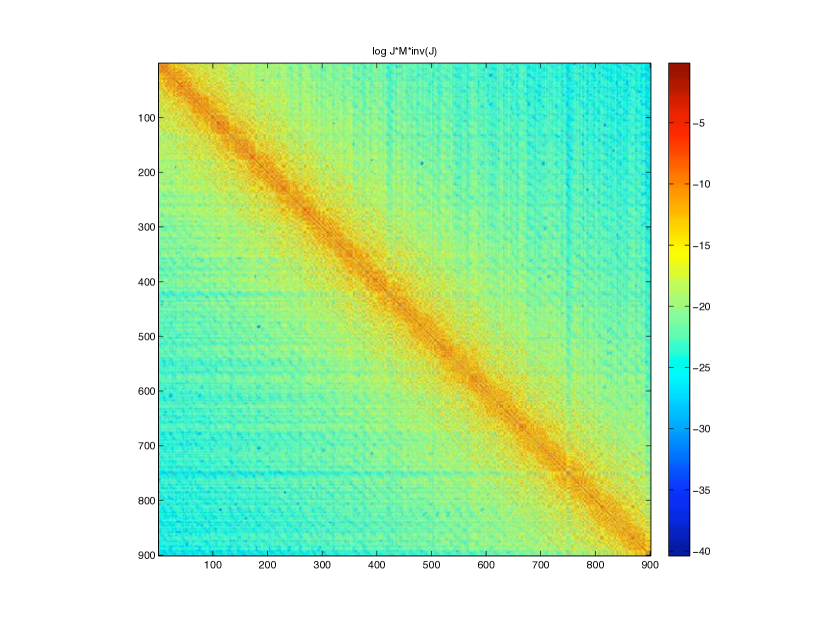
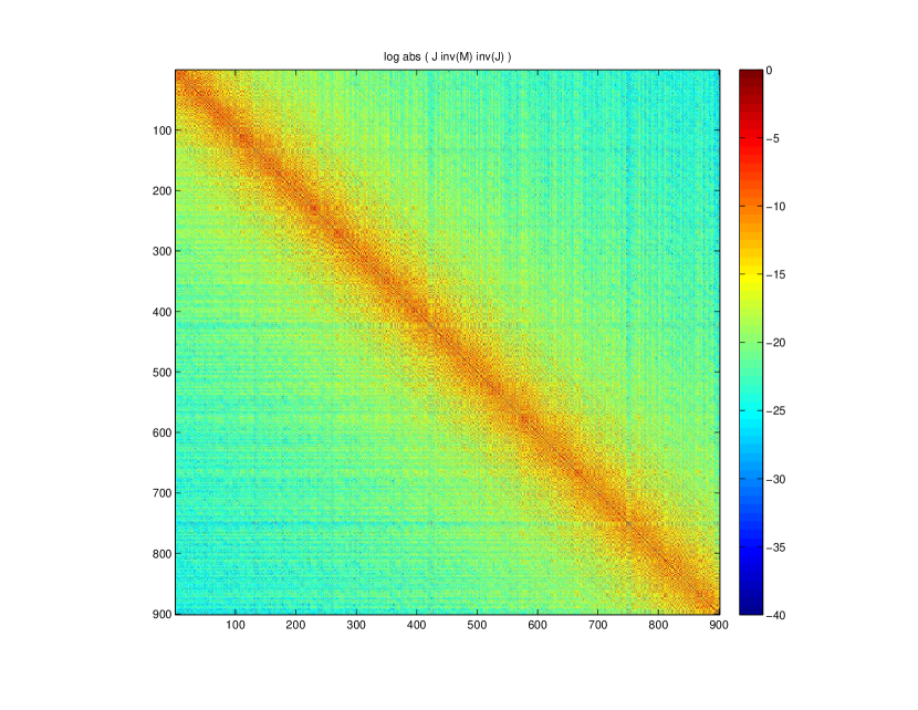
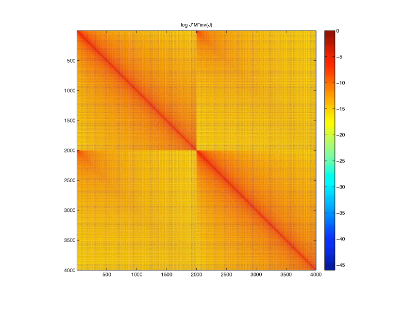
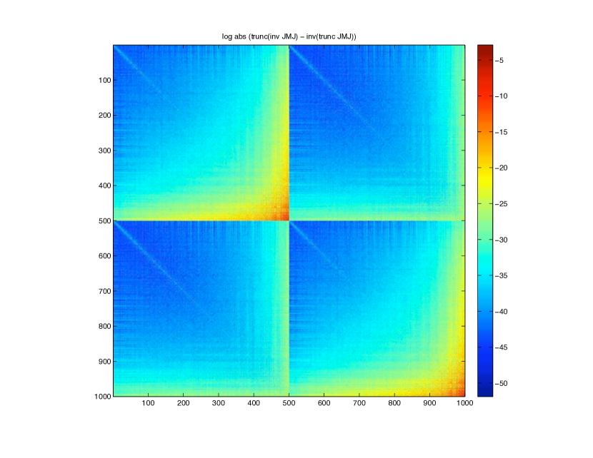
Figure 3 shows the log of JMT,ωJ1𝐽subscript𝑀𝑇𝜔superscript𝐽1JM_{T,\omega}J^{-1} coefficients and illustrates the decay estimates (51) and (52). A zoom in is done in figure 4, so that we can observe more precisely (51). In particular we can notice that the distribution of the coefficients along the diagonal of the matrix is not regular. Figure 5 presents the same zoom for JMT,ω1J1𝐽superscriptsubscript𝑀𝑇𝜔1superscript𝐽1JM_{T,\omega}^{-1}J^{-1}. This gives an illustration of the matrix structure of a microlocal operator. Figure 6 represents the log of JMT,ωJ1𝐽subscript𝑀𝑇𝜔superscript𝐽1JM_{T,\omega}J^{-1} coefficients without smoothing. And finally, figure 7 gives a view of the convergence of our Galerkin approximation, as it presents the matrix entries of J(ΛωMT,ω1)J1𝐽subscriptΛ𝜔superscriptsubscript𝑀𝑇𝜔1superscript𝐽1J(\Lambda_{\omega}-M_{T,\omega}^{-1})J^{-1}, illustrating lemma 2, its proof, and lemma 3.
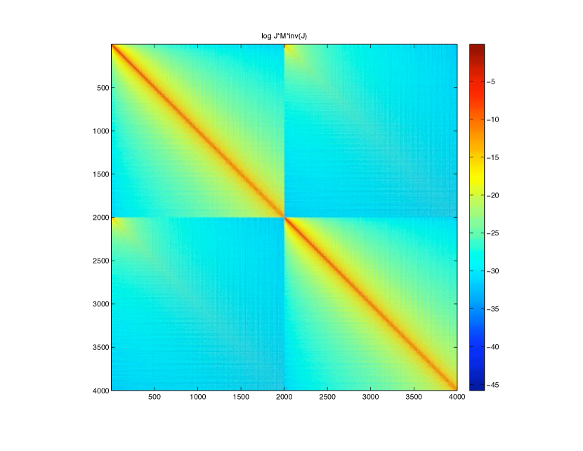
Refer to caption
Figure 3: View of the logarithm of the coefficients of the matrix JMTJ1𝐽subscript𝑀𝑇superscript𝐽1JM_{T}J^{-1}, for the square geometry, with smooth control. This illustrates decay estimates (51) and (52).
Refer to caption
Figure 4: View of the logarithm of the coefficients of the matrix JMTJ1𝐽subscript𝑀𝑇superscript𝐽1JM_{T}J^{-1}, for the square geometry, with smooth control (zoom). This illustrates decay estimate (51).
Refer to caption
Figure 5: View of the logarithm of the coefficients of the matrix JMT1J1𝐽superscriptsubscript𝑀𝑇1superscript𝐽1JM_{T}^{-1}J^{-1}, for the square geometry, with smooth control (zoom).
Refer to caption
Figure 6: View of the logarithm of the coefficients of the matrix JMTJ1𝐽subscript𝑀𝑇superscript𝐽1JM_{T}J^{-1}, for the square geometry, with non-smooth control. Note that the color scaling is the same as in Figure 3.
Refer to caption
Figure 7: View of the logarithm of the coefficients of the matrix J[((MT)1)ω((MT)ω)1]J1=J[Λω((MT)ω)1]J1𝐽delimited-[]subscriptsuperscriptsubscript𝑀𝑇1𝜔superscriptsubscriptsubscript𝑀𝑇𝜔1superscript𝐽1𝐽delimited-[]subscriptΛ𝜔superscriptsubscriptsubscript𝑀𝑇𝜔1superscript𝐽1J\left[((M_{T})^{-1})_{\omega}-((M_{T})_{\omega})^{-1}\right]J^{-1}=J\left[\Lambda_{\omega}-((M_{T})_{\omega})^{-1}\right]J^{-1}, for the square geometry, with smooth control. The MTsubscript𝑀𝑇M_{T} matrix is computed with 2000 eigenvalues, the cutoff frequency ω𝜔\omega being associated with the 500th eigenvalue.

2.4 Computation of the discrete control operator

For any real ω𝜔\omega, let N(ω)=sup{n,ωnω}𝑁𝜔supremum𝑛subscript𝜔𝑛𝜔N(\omega)=\sup\{n,\omega_{n}\leq\omega\}. Then the dimension of the vector space Lω2subscriptsuperscript𝐿2𝜔L^{2}_{\omega} is equal to N(ω)𝑁𝜔N(\omega). Let us define the following (ϕj)1j2N(ω)subscriptsubscriptitalic-ϕ𝑗1𝑗2𝑁𝜔(\phi_{j})_{1\leq j\leq 2N(\omega)}:

{ϕj=ejωjfor1jN(ω)ϕj=ejN(ω)forN(ω)+1j2N(ω)casessubscriptitalic-ϕ𝑗subscript𝑒𝑗subscript𝜔𝑗for1𝑗𝑁𝜔subscriptitalic-ϕ𝑗subscript𝑒𝑗𝑁𝜔for𝑁𝜔1𝑗2𝑁𝜔\left\{\begin{array}[]{rcl}\phi_{j}={e_{j}\over\omega_{j}}&\textrm{for}&1\leq j\leq N(\omega)\\ \phi_{j}=e_{j-N(\omega)}&\textrm{for}&N(\omega)+1\leq j\leq 2N(\omega)\end{array}\right. (53)

Then (ϕj)1j2N(ω)subscriptsubscriptitalic-ϕ𝑗1𝑗2𝑁𝜔(\phi_{j})_{1\leq j\leq 2N(\omega)} is an orthonormal basis of the Hilbert space Hω=Πω(H01(Ω)L2(Ω))subscript𝐻𝜔subscriptΠ𝜔direct-sumsubscriptsuperscript𝐻10Ωsuperscript𝐿2ΩH_{\omega}=\Pi_{\omega}(H^{1}_{0}(\Omega)\oplus L^{2}(\Omega)).

In this section we compute explicitly (MTϕl|ϕk)Hsubscriptconditionalsubscript𝑀𝑇subscriptitalic-ϕ𝑙subscriptitalic-ϕ𝑘𝐻\big{(}M_{T}\phi_{l}|\phi_{k}\big{)}_{H} for all 1k,l2N(ω)formulae-sequence1𝑘𝑙2𝑁𝜔1\leq k,l\leq 2N(\omega). We recall

eisA[ei0]=[cos(sωi)ei(x)ωisin(sωi)ei(x)]eisA[0ei]=[sin(sωi)ei(x)/ωicos(sωi)ei(x)]superscript𝑒𝑖𝑠𝐴delimited-[]subscript𝑒𝑖0delimited-[]𝑠subscript𝜔𝑖subscript𝑒𝑖𝑥subscript𝜔𝑖𝑠subscript𝜔𝑖subscript𝑒𝑖𝑥superscript𝑒𝑖𝑠𝐴delimited-[]0subscript𝑒𝑖delimited-[]𝑠subscript𝜔𝑖subscript𝑒𝑖𝑥subscript𝜔𝑖𝑠subscript𝜔𝑖subscript𝑒𝑖𝑥\begin{array}[]{rcl}e^{isA}\left[\begin{array}[]{l}e_{i}\\ 0\end{array}\right]&=&\left[\begin{array}[]{l}\cos(s\omega_{i})e_{i}(x)\\ -\omega_{i}\sin(s\omega_{i})e_{i}(x)\end{array}\right]\vskip 6.0pt plus 2.0pt minus 2.0pt\\ e^{isA}\left[\begin{array}[]{l}0\\ e_{i}\end{array}\right]&=&\left[\begin{array}[]{l}\sin(s\omega_{i})e_{i}(x)/\omega_{i}\\ \cos(s\omega_{i})e_{i}(x)\end{array}\right]\end{array} (54)

We now compute the coefficients of the MTsubscript𝑀𝑇M_{T} matrix, namely MTn,m=(MTϕn|ϕm)Hsubscriptsubscript𝑀𝑇𝑛𝑚subscriptconditionalsubscript𝑀𝑇subscriptitalic-ϕ𝑛subscriptitalic-ϕ𝑚𝐻{M_{T}}_{n,m}=\big{(}M_{T}\phi_{n}|\phi_{m}\big{)}_{H}:

MTn,m=(MTϕn|ϕm)H=0T(eisABBeisAϕn|ϕm)H𝑑t=0T((000χ2)eisAϕn|eisAϕm)H𝑑tsubscriptsubscript𝑀𝑇𝑛𝑚subscriptconditionalsubscript𝑀𝑇subscriptitalic-ϕ𝑛subscriptitalic-ϕ𝑚𝐻missing-subexpressionsuperscriptsubscript0𝑇subscriptconditionalsuperscript𝑒𝑖𝑠𝐴𝐵superscript𝐵superscript𝑒𝑖𝑠𝐴subscriptitalic-ϕ𝑛subscriptitalic-ϕ𝑚𝐻differential-d𝑡missing-subexpressionsuperscriptsubscript0𝑇subscriptconditional000superscript𝜒2superscript𝑒𝑖𝑠𝐴subscriptitalic-ϕ𝑛superscript𝑒𝑖𝑠𝐴subscriptitalic-ϕ𝑚𝐻differential-d𝑡\begin{array}[]{rcl}{M_{T}}_{n,m}&=&\big{(}M_{T}\phi_{n}|\phi_{m}\big{)}_{H}\\ &=&\int_{0}^{T}\big{(}e^{isA}BB^{*}e^{-isA}\phi_{n}|\phi_{m}\big{)}_{H}\,dt\\ &=&\int_{0}^{T}\big{(}\left(\begin{array}[]{ll}0&0\\ 0&\chi^{2}\end{array}\right)e^{-isA}\phi_{n}|e^{-isA}\phi_{m}\big{)}_{H}\,dt\end{array} (55)

We now have to distinguish four cases, depending on m,n𝑚𝑛m,n being smaller or larger than N(ω)𝑁𝜔N(\omega). For the case (m,n)N(ω)𝑚𝑛𝑁𝜔(m,n)\leq N(\omega) we have:

MTn,m=0T((000χ2)eisAϕn|eisAϕm)H𝑑s=0T((000χ2)[cos(sωn)fn(x)ωnsin(sωn)fn(x)]|[cos(sωm)fm(x)ωmsin(sωm)fm(x)])H𝑑s=0T([0ωnχ2sin(sωn)fn(x)]|[cos(sωn)fm(x)ωmsin(sωm)fm(x)])H𝑑s=0T((ψ(t)χ0(x))2ωnsin(sωn)fn(x)|ωmsin(sωm)fm(x))L2(Ω)𝑑s=0Tψ2sin(sωn)sin(sωm)𝑑sΩχ02en(x)em(x)𝑑x=an,mGn,msubscriptsubscript𝑀𝑇𝑛𝑚superscriptsubscript0𝑇subscriptconditional000superscript𝜒2superscript𝑒𝑖𝑠𝐴subscriptitalic-ϕ𝑛superscript𝑒𝑖𝑠𝐴subscriptitalic-ϕ𝑚𝐻differential-d𝑠missing-subexpressionsuperscriptsubscript0𝑇subscriptconditional000superscript𝜒2delimited-[]𝑠subscript𝜔𝑛subscript𝑓𝑛𝑥subscript𝜔𝑛𝑠subscript𝜔𝑛subscript𝑓𝑛𝑥delimited-[]𝑠subscript𝜔𝑚subscript𝑓𝑚𝑥subscript𝜔𝑚𝑠subscript𝜔𝑚subscript𝑓𝑚𝑥𝐻differential-d𝑠missing-subexpressionsuperscriptsubscript0𝑇subscriptconditionaldelimited-[]0subscript𝜔𝑛superscript𝜒2𝑠subscript𝜔𝑛subscript𝑓𝑛𝑥delimited-[]𝑠subscript𝜔𝑛subscript𝑓𝑚𝑥subscript𝜔𝑚𝑠subscript𝜔𝑚subscript𝑓𝑚𝑥𝐻differential-d𝑠missing-subexpressionsuperscriptsubscript0𝑇subscriptconditionalsuperscript𝜓𝑡subscript𝜒0𝑥2subscript𝜔𝑛𝑠subscript𝜔𝑛subscript𝑓𝑛𝑥subscript𝜔𝑚𝑠subscript𝜔𝑚subscript𝑓𝑚𝑥superscript𝐿2Ωdifferential-d𝑠missing-subexpressionsuperscriptsubscript0𝑇superscript𝜓2𝑠subscript𝜔𝑛𝑠subscript𝜔𝑚differential-d𝑠subscriptΩsuperscriptsubscript𝜒02subscript𝑒𝑛𝑥subscript𝑒𝑚𝑥differential-d𝑥missing-subexpressionsubscript𝑎𝑛𝑚subscript𝐺𝑛𝑚\begin{array}[]{rcl}{M_{T}}_{n,m}&=&\int_{0}^{T}\big{(}\left(\begin{array}[]{ll}0&0\\ 0&\chi^{2}\end{array}\right)e^{-isA}\phi_{n}|e^{-isA}\phi_{m}\big{)}_{H}\,ds\vskip 6.0pt plus 2.0pt minus 2.0pt\\ &=&\int_{0}^{T}\big{(}\left(\begin{array}[]{ll}0&0\\ 0&\chi^{2}\end{array}\right)\left[\begin{array}[]{l}\cos(s\omega_{n})f_{n}(x)\\ \omega_{n}\sin(s\omega_{n})f_{n}(x)\end{array}\right]|\left[\begin{array}[]{l}\cos(s\omega_{m})f_{m}(x)\\ \omega_{m}\sin(s\omega_{m})f_{m}(x)\end{array}\right]\big{)}_{H}\,ds\vskip 6.0pt plus 2.0pt minus 2.0pt\\ &=&\int_{0}^{T}\big{(}\left[\begin{array}[]{l}0\\ \omega_{n}\chi^{2}\sin(s\omega_{n})f_{n}(x)\end{array}\right]|\left[\begin{array}[]{l}\cos(s\omega_{n})f_{m}(x)\\ \omega_{m}\sin(s\omega_{m})f_{m}(x)\end{array}\right]\big{)}_{H}\,ds\vskip 6.0pt plus 2.0pt minus 2.0pt\\ &=&\int_{0}^{T}((\psi(t)\chi_{0}(x))^{2}\omega_{n}\sin(s\omega_{n})f_{n}(x)|\omega_{m}\sin(s\omega_{m})f_{m}(x))_{L^{2}(\Omega)}\,ds\vskip 6.0pt plus 2.0pt minus 2.0pt\\ &=&\int_{0}^{T}\psi^{2}\sin(s\omega_{n})\sin(s\omega_{m})\,ds\int_{\Omega}\chi_{0}^{2}e_{n}(x)e_{m}(x)\,dx\vskip 6.0pt plus 2.0pt minus 2.0pt\\ &=&a_{n,m}G_{n,m}\end{array} (56)

where

an,m=0Tψ2sin(sωm)sin(sωn)𝑑ssubscript𝑎𝑛𝑚superscriptsubscript0𝑇superscript𝜓2𝑠subscript𝜔𝑚𝑠subscript𝜔𝑛differential-d𝑠a_{n,m}=\int_{0}^{T}\psi^{2}\sin(s\omega_{m})\sin(s\omega_{n})\,ds (57)

and

Gn,m=Ωχ02(x)em(x)en(x)𝑑xsubscript𝐺𝑛𝑚subscriptΩsuperscriptsubscript𝜒02𝑥subscript𝑒𝑚𝑥subscript𝑒𝑛𝑥differential-d𝑥G_{n,m}=\int_{\Omega}\chi_{0}^{2}(x)\,e_{m}(x)\,e_{n}(x)\,dx (58)

Similarly, for the case n>N(ω)𝑛𝑁𝜔n>N(\omega), mN(ω)𝑚𝑁𝜔m\leq N(\omega) we have:

MTn,m=0T((000χ2)eisAϕn|eisAϕm)H𝑑s=0T((000χ2)[sin(sωn)fn(x)/ωncos(sωn)fn(x)]|[cos(sωm)fm(x)ωmsin(sωm)fm(x)])H𝑑s=0T([0χ2cos(sωn)fn(x)]|[cos(sωn)fm(x)ωmsin(sωm)fm(x)])H𝑑s=0T(χ2cos(sωn)fn(x)|ωmsin(sωm)fm(x))L2(Ω)𝑑s=0Tψ2cos(sωn)sin(sωm)𝑑sΩχ02en(x)em(x)𝑑x=bn,mGn,msubscriptsubscript𝑀𝑇𝑛𝑚superscriptsubscript0𝑇subscriptconditional000superscript𝜒2superscript𝑒𝑖𝑠𝐴subscriptitalic-ϕ𝑛superscript𝑒𝑖𝑠𝐴subscriptitalic-ϕ𝑚𝐻differential-d𝑠missing-subexpressionsuperscriptsubscript0𝑇subscriptconditional000superscript𝜒2delimited-[]𝑠subscript𝜔𝑛subscript𝑓𝑛𝑥subscript𝜔𝑛𝑠subscript𝜔𝑛subscript𝑓𝑛𝑥delimited-[]𝑠subscript𝜔𝑚subscript𝑓𝑚𝑥subscript𝜔𝑚𝑠subscript𝜔𝑚subscript𝑓𝑚𝑥𝐻differential-d𝑠missing-subexpressionsuperscriptsubscript0𝑇subscriptconditionaldelimited-[]0superscript𝜒2𝑠subscript𝜔𝑛subscript𝑓𝑛𝑥delimited-[]𝑠subscript𝜔𝑛subscript𝑓𝑚𝑥subscript𝜔𝑚𝑠subscript𝜔𝑚subscript𝑓𝑚𝑥𝐻differential-d𝑠missing-subexpressionsuperscriptsubscript0𝑇subscriptconditionalsuperscript𝜒2𝑠subscript𝜔𝑛subscript𝑓𝑛𝑥subscript𝜔𝑚𝑠subscript𝜔𝑚subscript𝑓𝑚𝑥superscript𝐿2Ωdifferential-d𝑠missing-subexpressionsuperscriptsubscript0𝑇superscript𝜓2𝑠subscript𝜔𝑛𝑠subscript𝜔𝑚differential-d𝑠subscriptΩsuperscriptsubscript𝜒02subscript𝑒𝑛𝑥subscript𝑒𝑚𝑥differential-d𝑥missing-subexpressionsubscript𝑏𝑛𝑚subscript𝐺𝑛𝑚\begin{array}[]{rcl}{M_{T}}_{n,m}&=&\int_{0}^{T}\big{(}\left(\begin{array}[]{ll}0&0\\ 0&\chi^{2}\end{array}\right)e^{-isA}\phi_{n}|e^{-isA}\phi_{m}\big{)}_{H}\,ds\vskip 6.0pt plus 2.0pt minus 2.0pt\\ &=&\int_{0}^{T}\big{(}\left(\begin{array}[]{ll}0&0\\ 0&\chi^{2}\end{array}\right)\left[\begin{array}[]{l}\sin(s\omega_{n})f_{n}(x)/\omega_{n}\\ \cos(s\omega_{n})f_{n}(x)\end{array}\right]|\left[\begin{array}[]{l}\cos(s\omega_{m})f_{m}(x)\\ \omega_{m}\sin(s\omega_{m})f_{m}(x)\end{array}\right]\big{)}_{H}\,ds\vskip 6.0pt plus 2.0pt minus 2.0pt\\ &=&\int_{0}^{T}\big{(}\left[\begin{array}[]{l}0\\ \chi^{2}\cos(s\omega_{n})f_{n}(x)\end{array}\right]|\left[\begin{array}[]{l}\cos(s\omega_{n})f_{m}(x)\\ \omega_{m}\sin(s\omega_{m})f_{m}(x)\end{array}\right]\big{)}_{H}\,ds\vskip 6.0pt plus 2.0pt minus 2.0pt\\ &=&\int_{0}^{T}(\chi^{2}\cos(s\omega_{n})f_{n}(x)|\omega_{m}\sin(s\omega_{m})f_{m}(x))_{L^{2}(\Omega)}\,ds\vskip 6.0pt plus 2.0pt minus 2.0pt\\ &=&\int_{0}^{T}\psi^{2}\cos(s\omega_{n})\sin(s\omega_{m})\,ds\int_{\Omega}\chi_{0}^{2}e_{n}(x)e_{m}(x)\,dx\vskip 6.0pt plus 2.0pt minus 2.0pt\\ &=&b_{n,m}G_{n,m}\end{array} (59)

where

bn,m=0Tψ2cos(sωn)sin(sωm)𝑑ssubscript𝑏𝑛𝑚superscriptsubscript0𝑇superscript𝜓2𝑠subscript𝜔𝑛𝑠subscript𝜔𝑚differential-d𝑠b_{n,m}=\int_{0}^{T}\psi^{2}\cos(s\omega_{n})\sin(s\omega_{m})\,ds (60)

For nN(ω)𝑛𝑁𝜔n\leq N(\omega) and m>N(ω)𝑚𝑁𝜔m>N(\omega) we get:

MTn,m=cn,mGn,msubscriptsubscript𝑀𝑇𝑛𝑚subscript𝑐𝑛𝑚subscript𝐺𝑛𝑚\begin{array}[]{rcl}{M_{T}}_{n,m}&=&c_{n,m}G_{n,m}\end{array} (61)

where

cn,m=bm,n=0Tψ2cos(sωm)sin(sωn)𝑑ssubscript𝑐𝑛𝑚subscript𝑏𝑚𝑛superscriptsubscript0𝑇superscript𝜓2𝑠subscript𝜔𝑚𝑠subscript𝜔𝑛differential-d𝑠c_{n,m}=b_{m,n}=\int_{0}^{T}\psi^{2}\cos(s\omega_{m})\sin(s\omega_{n})\,ds (62)

And for m,n>N(ω)𝑚𝑛𝑁𝜔m,n>N(\omega):

MTn,m=dn,mGn,msubscriptsubscript𝑀𝑇𝑛𝑚subscript𝑑𝑛𝑚subscript𝐺𝑛𝑚\begin{array}[]{rcl}{M_{T}}_{n,m}&=&d_{n,m}G_{n,m}\end{array} (63)

where

dn,m=0Tψ2cos(sωm)cos(sωn)𝑑ssubscript𝑑𝑛𝑚superscriptsubscript0𝑇superscript𝜓2𝑠subscript𝜔𝑚𝑠subscript𝜔𝑛differential-d𝑠d_{n,m}=\int_{0}^{T}\psi^{2}\cos(s\omega_{m})\cos(s\omega_{n})\,ds (64)

The above integrals have to be implemented carefully when |ωnωm|subscript𝜔𝑛subscript𝜔𝑚|\omega_{n}-\omega_{m}| is small, even when ψ(t)=1𝜓𝑡1\psi(t)=1.

3 Numerical setup and validation

3.1 Geometries and control domains

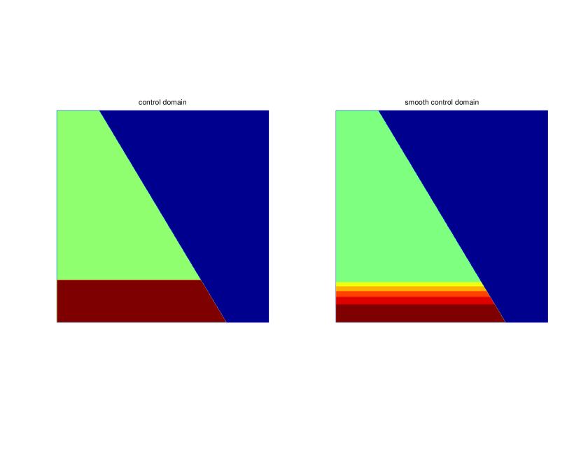
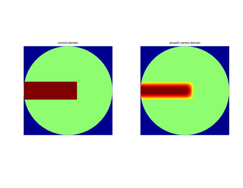
The code we implemented allows us to choose the two-dimensional domain ΩΩ\Omega, as well as the control domain U𝑈U. In the sequel, we will present some results with three different geometries: square, disc and trapezoid. For each geometry, we have chosen a reference shape of control domain. It consists of the neighborhood of two adjacent sides of the boundary (in the square), of a radius (in the disc), of the base side (in the trapezoid). Then we adjust the width of the control domain, and also its smoothness (see next paragraph). Figures 8, 9 and 10 present these domains, and their respective control domains, either non-smooth (left panels) or smooth (right panels).
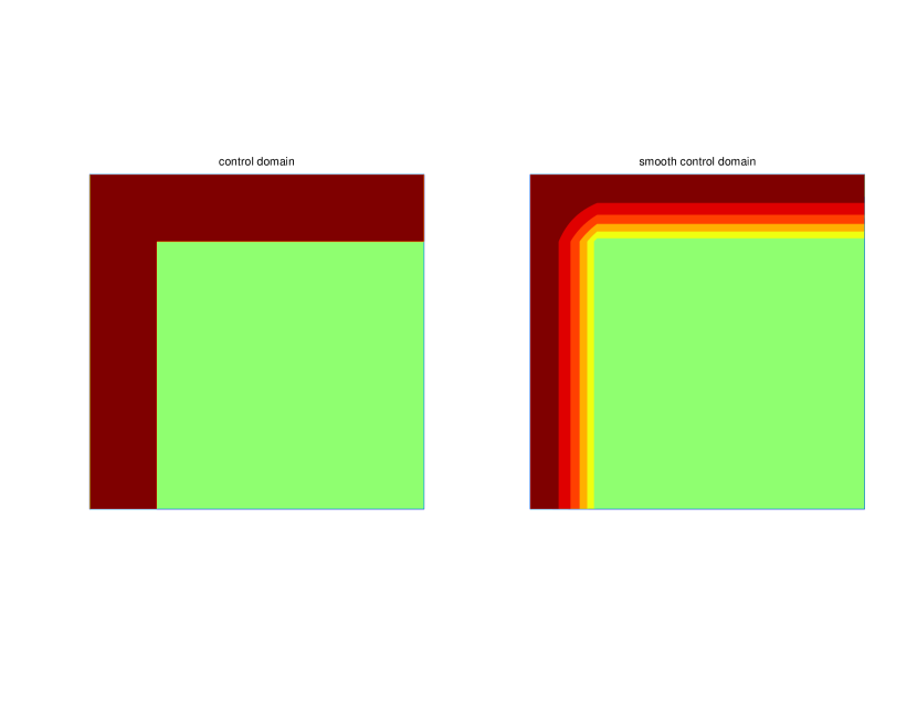
Refer to caption
Figure 8: Domain and example of a control domain for the square, with smoothing in space (right panel) or without (left panel).
Refer to caption
Figure 9: Domain and example of a control domain for the disc, with smoothing in space (right panel) or without (left panel).
Refer to caption
Figure 10: Domain and example of a control domain for the trapezoid, with smoothing in space (right panel) or without (left panel).

3.2 Time and space smoothing

We will investigate the influence of the regularity of the function χ(t,x)=ψ(t)χ0(x)𝜒𝑡𝑥𝜓𝑡subscript𝜒0𝑥\chi(t,x)=\psi(t)\chi_{0}(x). Different options have been set.

Space-smoothing.

The integral (58) defining Gn,msubscript𝐺𝑛𝑚G_{n,m} features χ0subscript𝜒0\chi_{0}. In the literature we find χ0=𝟏Usubscript𝜒0subscript1𝑈\chi_{0}={\bf 1}_{U}, so that

Gn,m=Uen(x)em(x)𝑑xsubscript𝐺𝑛𝑚subscript𝑈subscript𝑒𝑛𝑥subscript𝑒𝑚𝑥differential-d𝑥G_{n,m}=\int_{U}e_{n}(x)\,e_{m}(x)\,dx (65)

In [DL09] the authors show that a smooth χ02superscriptsubscript𝜒02\chi_{0}^{2} leads to a more regular control (see also theorem 3 and lemma 3). Thus for each control domain U𝑈U we implemented both smooth and non-smooth (constant) cases. The different implementations of χ0subscript𝜒0\chi_{0} are:

  • constant case: χ0(x,y)=𝟏Usubscript𝜒0𝑥𝑦subscript1𝑈\chi_{0}(x,y)={\bf 1}_{U},

  • “smooth” case: χ0(x,y)subscript𝜒0𝑥𝑦\chi_{0}(x,y) has the same support of U𝑈U, the width a𝑎a of the domain {xΩ,0<χ0(x)<1}formulae-sequence𝑥Ω0subscript𝜒0𝑥1\{x\in\Omega,0<\chi_{0}(x)<1\} is adjustable, and on this domain χ𝜒\chi is a polynomial of degree 2. For example, in the square we have:

    χ0(x,y)=𝟏U[1(𝟏xa+x2a2.1x<a)(𝟏y1a+(1y)2a2.1y>1a)]\begin{array}[]{rcl}\chi_{0}(x,y)&=&{\bf 1}_{U}\Big{[}1-\Big{(}{\bf 1}_{x\geq a}+\frac{x^{2}}{a^{2}}.{\bf 1}_{x<a}\Big{)}\\ &&\qquad\quad\Big{(}{\bf 1}_{y\leq 1-a}+\frac{(1-y)^{2}}{a^{2}}.{\bf 1}_{y>1-a}\Big{)}\Big{]}\end{array} (66)
Time-smoothing.

Similarly, the time integrals (57,60,62,64) defining a𝑎a, b𝑏b, c𝑐c and d𝑑d features ψ(t)𝜓𝑡\psi(t), which is commonly chosen as 𝟏[0,T]subscript10𝑇{\bf 1}_{[0,T]}. As previously, better results are expected with a smooth ψ(t)𝜓𝑡\psi(t). In the code, the integrals (57,60,62,64) are computed explicitly, the different implementations of ψ𝜓\psi being:

  • constant case ψ=𝟏[0,T]𝜓subscript10𝑇\psi={\bf 1}_{[0,T]},

  • “smooth case”

    ψ(t)=4t(Tt)T2𝟏[0,T]𝜓𝑡4𝑡𝑇𝑡superscript𝑇2subscript10𝑇\psi(t)=\frac{4t(T-t)}{T^{2}}{\bf 1}_{[0,T]} (67)

3.3 Validation of the eigenvalues computation

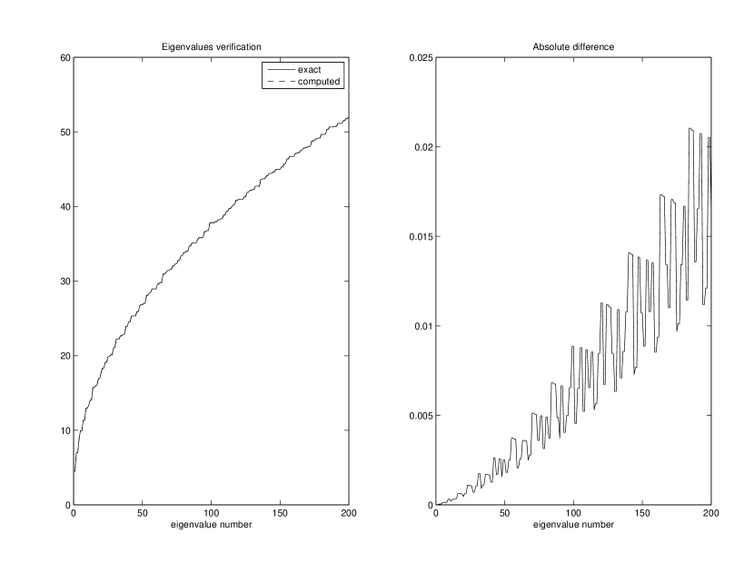
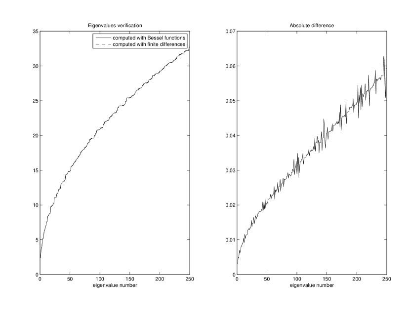
The code we implemented has a wide range of geometries for ΩΩ\Omega. As it is a spectral-Galerkin method, it requires the accurate computation of eigenvalues and eigenvectors. We used Matlab eigs444www.mathworks.com/access/helpdesk/help/techdoc/ref/eigs.html function. Figure 11 shows the comparison between the first 200 exact eigenvalues in the square, and those computed by Matlab with 500×500500500500\times 500 grid-points. Figure 12 presents the same comparison in the disc, for 250 eigenvalues, the “exact” ones being computed as zeros of Bessel function.
Refer to caption
Figure 11: Verification of the eigenvalues computation in the square: exact and finite-differences-computed eigenvalues (left panel), and their absolute difference (right panel).
Refer to caption
Figure 12: Verification of the eigenvalues computation in the disc: eigenvalues computed either as zeros of Bessel functions or with finite differences (left panel), and their absolute difference (right panel).

3.4 Reconstruction error.

In the sequel, we will denote the input data u=(u0,u1)𝑢subscript𝑢0subscript𝑢1u=(u_{0},u_{1}), and its image by the control map w=(w0,w1)=Λ(u0,u1)𝑤subscript𝑤0subscript𝑤1Λsubscript𝑢0subscript𝑢1w=(w_{0},w_{1})=\Lambda(u_{0},u_{1}), which will often be called the “control”. We recall from section 2.1 that for a given data u=(u0,u1)𝑢subscript𝑢0subscript𝑢1u=(u_{0},u_{1}) to be reconstructed at time T𝑇T, the optimal control v(t)𝑣𝑡v(t) is given by

v(t)=χtei(Tt)Aw=χtei(Tt)AΛ(u)𝑣𝑡𝜒subscript𝑡superscript𝑒𝑖𝑇𝑡𝐴𝑤𝜒subscript𝑡superscript𝑒𝑖𝑇𝑡𝐴Λ𝑢v(t)=\chi\partial_{t}e^{-i(T-t)A}w=\chi\partial_{t}e^{-i(T-t)A}\Lambda(u) (68)

Then, solving the wave equations (2) forward, with null initial conditions and χv𝜒𝑣\chi v as a forcing source, we reach y=(y0,y1)𝑦subscript𝑦0subscript𝑦1y=(y_{0},y_{1}) in time T𝑇T. Should the experiment be perfect, we would have (y0,y1)=(u0,u1)subscript𝑦0subscript𝑦1subscript𝑢0subscript𝑢1(y_{0},y_{1})=(u_{0},u_{1}). The reconstruction error is then by definition:

E=u0y0H1(Ω)2+u1y1L2(Ω)2u0H1(Ω)2+u1L2(Ω)2𝐸subscriptsuperscriptnormsubscript𝑢0subscript𝑦02superscript𝐻1Ωsubscriptsuperscriptnormsubscript𝑢1subscript𝑦12superscript𝐿2Ωsubscriptsuperscriptnormsubscript𝑢02superscript𝐻1Ωsubscriptsuperscriptnormsubscript𝑢12superscript𝐿2ΩE=\sqrt{\frac{\|u_{0}-y_{0}\|^{2}_{H^{1}(\Omega)}+\|u_{1}-y_{1}\|^{2}_{L^{2}(\Omega)}}{\|u_{0}\|^{2}_{H^{1}(\Omega)}+\|u_{1}\|^{2}_{L^{2}(\Omega)}}} (69)

3.5 Validation for the square geometry

3.5.1 Finite differences versus exact eigenvalues

In this paragraph, we compare various outputs for our spectral method, when the eigenvalues and eigenvectors are computed either with finite-differences or with exact formulas. In this first experiment, we have N×N=500×500𝑁𝑁500500N\times N=500\times 500 grid-points and we use Ne=100subscript𝑁𝑒100N_{e}=100 eigenvalues to compute the G𝐺G and MTsubscript𝑀𝑇M_{T} matrices. The data (u0,u1)subscript𝑢0subscript𝑢1(u_{0},u_{1}) is as follows:

{u0=e50u1=0casessubscript𝑢0subscript𝑒50subscript𝑢10\left\{\begin{array}[]{rcl}u_{0}&=&e_{50}\\ u_{1}&=&0\end{array}\right. (70)

Where ensubscript𝑒𝑛e_{n} denotes the n𝑛n-th exact eigenvector. The control time T𝑇T is equal to 3, the control domain U𝑈U is 0.2 wide, and we do not use any smoothing. For reconstruction we use 2000 eigenvalues and eigenvectors.
Table 1 shows the condition number of the MTsubscript𝑀𝑇M_{T} matrices, and reconstruction errors, which are very similar for both experiments.

Eigenvalues computation Condition Number Reconstruction error
Finite differences 7.4 1.8 %
Exact 7.5 1.6 %
Table 1: Validation experiments in the square: Condition numbers and validation errors for a 100-eigenvalues-experiment in the square (without smoothing), where the eigenvalues are exact or computed thanks to finite differences.

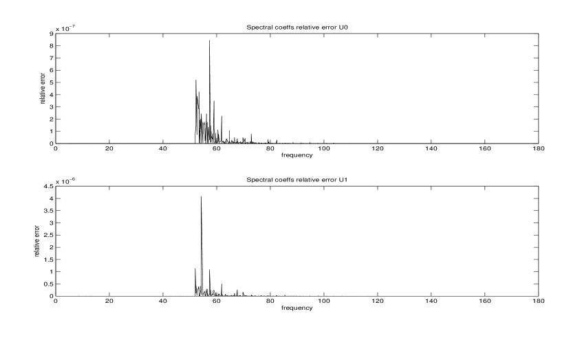
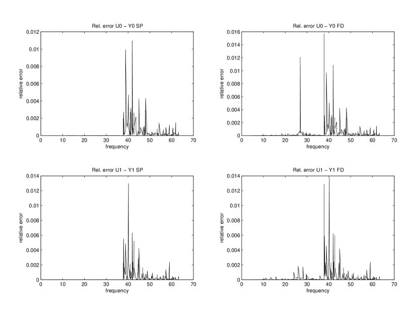
Figure 13 shows the relative reconstruction error between the data u𝑢u and the reconstructed y𝑦y for both experiments:

Relative reconstruction error SPn=|U0,nY0,nsp|U0+U1Relative reconstruction error FDn=|U0,nY0,nfd|U0+U1subscriptRelative reconstruction error SP𝑛subscript𝑈0𝑛subscriptsuperscript𝑌𝑠𝑝0𝑛normsubscript𝑈0subscript𝑈1subscriptRelative reconstruction error FD𝑛subscript𝑈0𝑛subscriptsuperscript𝑌𝑓𝑑0𝑛normsubscript𝑈0subscript𝑈1\begin{array}[]{rcl}\textrm{Relative reconstruction error SP}_{n}&=&\displaystyle\frac{|U_{0,n}-Y^{sp}_{0,n}|}{\|U_{0}+U_{1}\|}\\ \textrm{Relative reconstruction error FD}_{n}&=&\displaystyle\frac{|U_{0,n}-Y^{fd}_{0,n}|}{\|U_{0}+U_{1}\|}\end{array} (71)

and similarly for u1subscript𝑢1u_{1} and y1subscript𝑦1y_{1}, where U0,nsubscript𝑈0𝑛U_{0,n} is the n𝑛n-th spectral coefficient of the data u0subscript𝑢0u_{0}, Y0,nspsubscriptsuperscript𝑌𝑠𝑝0𝑛Y^{sp}_{0,n} is the n𝑛n-th spectral coefficient (in the basis (ϕj)subscriptitalic-ϕ𝑗(\phi_{j}) defined by formulas (53) in section 2.4) of the reconstructed y0subscript𝑦0y_{0} when the control w𝑤w is obtained thanks to exact eigenvalues and Y0,nfdsubscriptsuperscript𝑌𝑓𝑑0𝑛Y^{fd}_{0,n} is the n𝑛n-th spectral coefficient of y0subscript𝑦0y_{0} when the control w𝑤w is obtained thanks to finite differences eigenvalues. The norm U0+U1normsubscript𝑈0subscript𝑈1\|U_{0}+U_{1}\| in our basis (ϕj)subscriptitalic-ϕ𝑗(\phi_{j}) is given by:

U0+U12=n=1NeU0,n2+U1,n2superscriptnormsubscript𝑈0subscript𝑈12superscriptsubscript𝑛1subscript𝑁𝑒superscriptsubscript𝑈0𝑛2superscriptsubscript𝑈1𝑛2\|U_{0}+U_{1}\|^{2}=\sum_{n=1}^{N_{e}}U_{0,n}^{2}+U_{1,n}^{2} (72)

For exact eigenvalues, we can see that the errors are negligible on the first 100100100-th spectral coefficients, and quite small on the next ones. We have similar results for finite differences eigenvalues, except that we have an error on the 50-th coefficient. This error does not occur when the reconstruction is done with the same finite differences eigenvectors basis, and it can probably be explained as follows: to compute the reconstructed y𝑦y from the finite difference control w𝑤w, we first compute an approximation of w𝑤w as a function of (x,y)𝑥𝑦(x,y) (i.e. on the grid) from its spectral coefficients (on the finite differences eigenvectors basis), then we compute the coefficients of this function on the exact basis (thanks to a very simple integration formula). We thus introduce two sources of errors, projection on the grid and projection on the exact basis, which do not have anything to do with our spectral Galerkin method. Therefore we will not discuss the matter in further detail here.
Refer to caption
Figure 13: Validation experiments in the square: Relative errors between the spectral coefficients of the original function u𝑢u and the reconstructed function y𝑦y, computed with exact eigenvalues (left panels) or finite differences eigenvalues (right panels), for u0subscript𝑢0u_{0} and y0subscript𝑦0y_{0} (top panels) or u1subscript𝑢1u_{1} and y1subscript𝑦1y_{1} (bottom panels). The errors are plotted as a function of the frequency of the eigenvalues. The computation are performed with 100 eigenvalues, corresponding to a frequency of about 38, the reconstruction with 2000, corresponding to a frequency of about 160. For the readability of the figure, we plot only the major counterparts of the error, i.e. we stop the plot after frequency 63 (300th eigenvalue).

3.5.2 Impact of the number of eigenvalues

In this paragraph, we still use the same data (70), but the number of eigenvalues and eigenvectors Nesubscript𝑁𝑒N_{e} used to compute the MTsubscript𝑀𝑇M_{T} matrices is varying. Table 2 shows MTsubscript𝑀𝑇M_{T} condition numbers and reconstruction errors for various Nesubscript𝑁𝑒N_{e} with exact or finite-differences-computed eigenvalues. The reconstruction is still performed with 2000 exact eigenvalues. We can see that the finite differences eigenvalues lead to almost as good results as exact eigenvalues. We also observe in both cases the decrease of the reconstruction error with an increasing number of eigenvalues, as predicted in lemma 3. A 5% error is obtained with 70 eigenvalues (the input data being the 50-th eigenvalue), and 100 eigenvalues lead to less than 2%.

Condition Number Reconstruction error
Nesubscript𝑁𝑒N_{e} Exact Finite differences Exact Finite differences
52 6.5 6.4 29.2% 29.0%
55 6.6 6.6 17.7% 17.6%
60 6.6 6.6 17.3% 17.2%
70 7.1 7.0 4.9 % 5.0 %
80 7.3 7.2 3.2 % 3.3 %
100 7.5 7.4 1.6 % 1.8 %
200 8.3 8.3 0.5 % 1.0 %
300 8.8 0.3 %
500 9.5 0.2 %
Table 2: Validation experiments in the square: Condition numbers and validation errors for various numbers Nesubscript𝑁𝑒N_{e} of eigenvalues used to compute the control function, where the eigenvalues are exact or computed thanks to finite differences. The input data is the 505050-th eigenvalue, and the reconstruction is performed with 2000 eigenvalues.

4 Numerical experiments

4.1 Frequency localization

In this subsection, the geometry (square) as well as the number of eigenvalues used (200 for HUM, 2000 for verification) are fixed. Note also that in this paragraph we use only exact eigenvalues for HUM and verification.
The data is also fixed to a given eigenmode, that is:

u0=e50u1=0formulae-sequencesubscript𝑢0subscript𝑒50subscript𝑢10u_{0}=e_{50}\quad u_{1}=0 (73)

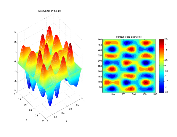
where ensubscript𝑒𝑛e_{n} is the n-th eigenvector of ΔΔ-\Delta on the square.

Refer to caption
Figure 14: Representation on the grid in 3D (left panel) or contour plot (right panel) of the 50-th eigenvector in the square.

The first output of interest is the spreading of w𝑤w spectral coefficients, compared to u𝑢u. Figure 15 shows the spectral coefficients of the input (u0,u1)subscript𝑢0subscript𝑢1(u_{0},u_{1}) and the control (w0,w1)subscript𝑤0subscript𝑤1(w_{0},w_{1}) with and without smoothing. As predicted by theorem 3 and lemma 3 we can see that the main coefficient of (w0,w1)subscript𝑤0subscript𝑤1(w_{0},w_{1}) is the 50-th of w0subscript𝑤0w_{0}, and also that the smoothing noticeably improves the localization of w𝑤w.

Refer to caption
Refer to caption
Figure 15: One-mode experiment in the square: localization of the Fourier frequences of (u0,u1)subscript𝑢0subscript𝑢1(u_{0},u_{1}) (dashed line) and (w0,w1)subscript𝑤0subscript𝑤1(w_{0},w_{1}) (solid line) for a given time T𝑇T and a given domain U𝑈U without smoothing (top) and with time- and space-smoothing (bottom). The x-coordinate represents the eigenvalues. The input data u0subscript𝑢0u_{0} is equal to the 50-th eigenvector, equal to an eigenvalue of about 26.8, and u1=0subscript𝑢10u_{1}=0.

Similarly we can look at the spectral coefficients of the reconstruction error. Figure 16 presents the reconstruction error (see paragraph 3.4 for a definition) with or without smoothing. We notice that the errors occur mostly above the cutoff frequency (used for MT,ωsubscript𝑀𝑇𝜔M_{T,\omega} computation, and thus for the control computation). Another important remark should be made here: the smoothing has a spectacular impact on the frequency localization of the error, as well as on the absolute value of the error (maximum of 2.103superscript2.1032.10^{-3} without smoothing, and 8.107superscript8.1078.10^{-7} with smoothing), as announced in theorem 3 and lemma 3.
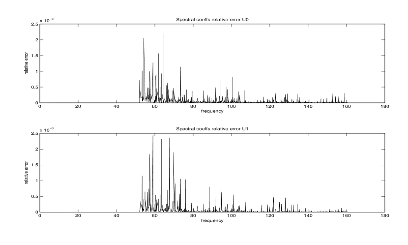
Refer to caption
Refer to caption
Figure 16: One-mode experiment in the square: localization of the Fourier coefficients of (u0y0,u1y1)subscript𝑢0subscript𝑦0subscript𝑢1subscript𝑦1(u_{0}-y_{0},u_{1}-y_{1}), where u𝑢u is the data and y𝑦y is the reconstructed function obtained from the control function w𝑤w, for a given time T𝑇T and a given domain U𝑈U without smoothing (top panels) and with time- and space-smoothing (bottom panels).
Remark 1

For other domains, such as the disc and trapezoid, as well as other one-mode input data, we obtain similar results. The results also remain the same if we permute u0𝑢0u0 and u1𝑢1u1, i.e. if we choose u0=0𝑢00u0=0 and u1𝑢1u1 equal to one fixed mode.

4.2 Space localization

4.2.1 Dirac experiments

In this section we investigate the localization in space. To do so, we use “Dirac” functions δ(x,y)=(x0,y0)subscript𝛿𝑥𝑦subscript𝑥0subscript𝑦0\delta_{(x,y)=(x_{0},y_{0})} as data, or more precisely truncations to a given cutoff frequency of Dirac functions:

{u0=i=1Nien(x0,y0)enu1=0casessubscript𝑢0superscriptsubscript𝑖1subscript𝑁𝑖subscript𝑒𝑛subscript𝑥0subscript𝑦0subscript𝑒𝑛subscript𝑢10\left\{\begin{array}[]{rcl}u_{0}&=&\sum_{i=1}^{N_{i}}e_{n}(x_{0},y_{0})\,e_{n}\\ u_{1}&=&0\end{array}\right. (74)

where Nisubscript𝑁𝑖N_{i} is the index corresponding to the chosen cutoff frequency, with Ni=100subscript𝑁𝑖100N_{i}=100 or 120120120 in the sequel. Figure 17 shows the data u0subscript𝑢0u_{0} and the control w0subscript𝑤0w_{0} in the square with exact eigenvalues, without smoothing, the results being similar with smoothing. We can see that the support of w0subscript𝑤0w_{0} is very similar to u0subscript𝑢0u_{0}’s. Figure 18 presents the reconstruction error associated to this experiment. We can see as before that the smoothing produces highly reduced errors.
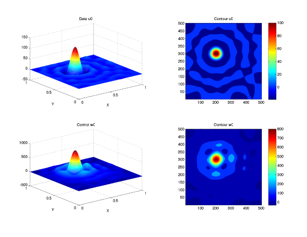
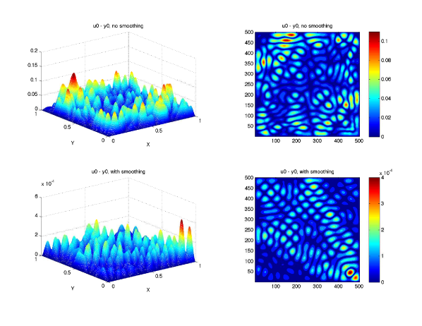
Refer to caption
Figure 17: Space localization of the data u0subscript𝑢0u_{0} (top panels) and the control w0subscript𝑤0w_{0} (bottom panels), for a Dirac experiment in the square, with exact eigenvalues. These plots correspond to an experiment without smoothing, but it is similar with smoothing. Left panels represent 3D view, and right panels show contour plots.
Refer to caption
Figure 18: Difference between the data u0subscript𝑢0u_{0} and the reconstructed function y0subscript𝑦0y_{0} without smoothing (top panels) and with smoothing (bottom panels) for a dirac experiment in the square, with exact eigenvalues. Left panels represent 3D view, and right panels show contour plots.

Similarly, we performed experiments with numerical approximation of a Dirac function as input data in the disc and in a trapezoid. Figures 19 and 20 present the space-localization of u0subscript𝑢0u_{0} and w0subscript𝑤0w_{0} without smoothing (we get similar results with smoothing). As previously, the control w0subscript𝑤0w_{0} is supported by roughly the same area than the input u0subscript𝑢0u_{0}. In the disc we can see a small disturbance, located in the symmetric area of the support of u0subscript𝑢0u_{0} with respect to the control domain U𝑈U. However, this error does not increase with Nisubscript𝑁𝑖N_{i}, as we can see in figure 21 (case Ni=200subscript𝑁𝑖200N_{i}=200) so it remains compatible with conjecture 1.
Figure 22 shows the reconstruction errors for these experiments, with or without smoothing. As before we notice the high improvement produced by the smoothing. We get similar errors in the trapezoid.
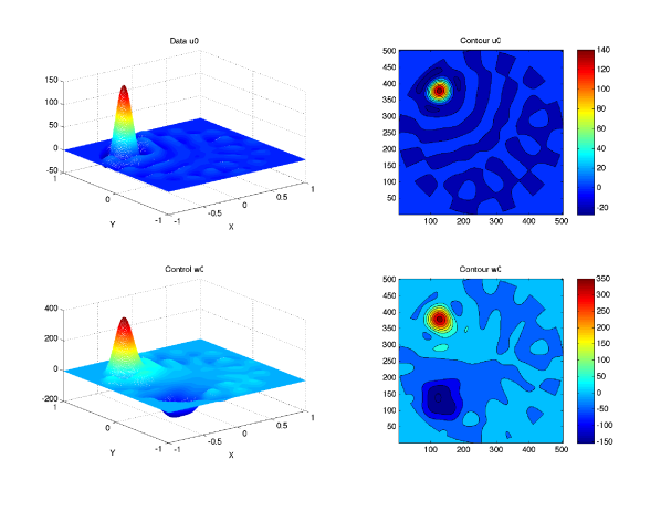
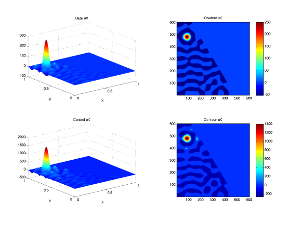
Refer to caption
Figure 19: Space localization of the data u0subscript𝑢0u_{0} (top panels) and the control w0subscript𝑤0w_{0} (bottom panels), for a dirac experiment in the disc. These plots correspond to an experiment without smoothing, but it is similar with smoothing. Left panels represent 3D view, and right panels show contour plots. In this experiment, the input data is defined with Ni=100subscript𝑁𝑖100N_{i}=100 eigenvectors.
Refer to caption
Figure 20: Space localization of the data u0subscript𝑢0u_{0} (top panels) and the control w0subscript𝑤0w_{0} (bottom panels), for a dirac experiment in the trapezoid. These plots correspond to an experiment without smoothing, but it is similar with smoothing. Left panels represent 3D view, and right panels show contour plots. In this experiment, the input data is defined with Ni=120subscript𝑁𝑖120N_{i}=120 eigenvectors.
Refer to caption
Figure 21: Space localization of the data u0subscript𝑢0u_{0} (top panels) and the control w0subscript𝑤0w_{0} (bottom panels), for a dirac experiment in the disc. These plots correspond to an experiment with smoothing, and it is similar without smoothing. Left panels represent 3D view, and right panels show contour plots. In this experiment, the input data is defined with Ni=200subscript𝑁𝑖200N_{i}=200 eigenvectors.
Refer to caption
Figure 22: Difference between the data u0subscript𝑢0u_{0} and the reconstructed function y0subscript𝑦0y_{0} for a dirac experiment in the disc without smoothing (top panels) and with time- and space-smoothing (bottom panels). Left panels represent 3D view, and right panels show contour plots. In this experiment, the input data is defined with Ni=100subscript𝑁𝑖100N_{i}=100 eigenvectors.

4.2.2 Box experiments in the square

In this paragraph we consider the case u0=𝟏boxsubscript𝑢0subscript1boxu_{0}={\bf 1}_{\textrm{box}}, where box=[0.6,0.8]×[0.2,0.4]box0.60.80.20.4\textrm{box}=[0.6,0.8]\times[0.2,0.4] is a box in the square. The control domain U𝑈U is 0.10.10.1 wide: U={x<0.1 and y>0.9}𝑈𝑥expectation0.1 and 𝑦0.9U=\{x<0.1\textrm{ and }y>0.9\}. These experiments were performed in the square with 1000 exact eigenvalues for the MTsubscript𝑀𝑇M_{T} matrix computation, the input data u0subscript𝑢0u_{0} being defined thanks to 800 eigenvalues. Figures 23 and 24 show the space localization of the data u0subscript𝑢0u_{0} and the control w0subscript𝑤0w_{0} without and with smoothing. As before we can notice that the space localization is preserved, and that with smoothing the support of w0subscript𝑤0w_{0} is more sharply defined. Figures 25 and 26 show the reconstruction errors for two different data, the first being the same as in figure 23, and the second being similar but rotated by π/4𝜋4\pi/4. We show here only the case with smoothing, the errors being larger but similarly shaped without. We can notice that the errors lows and highs are located on a lattice whose axes are parallel to the box sides. This is compatible with the structure of the wave-front set associated to both input data.
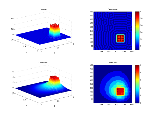
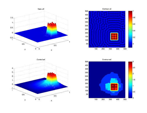
Refer to caption
Figure 23: Space localization of the control function w0subscript𝑤0w_{0} (bottom panels) with respect to the data u0subscript𝑢0u_{0} (top panels), in the square, without smoothing: 3D plots on the left, and contour plots on the right.
Refer to caption
Figure 24: Space localization of the control function w0subscript𝑤0w_{0} (bottom panels) with respect to the data u0subscript𝑢0u_{0} (top panels), in the square, with smoothing. Left panels represent 3D view, and right panels show contour plots.
Refer to caption
Figure 25: Difference between the data u0subscript𝑢0u_{0} and the reconstructed function y0subscript𝑦0y_{0} (top panels) and u1subscript𝑢1u_{1} and y1subscript𝑦1y_{1} (bottom panels) with smoothing in the square. The data is the identity function of a square whose edges are parallel to the x𝑥x and y𝑦y axes. Left panels represent 3D view, and right panels show contour plots.
Refer to caption
Figure 26: Difference between the data u0subscript𝑢0u_{0} and the reconstructed function y0subscript𝑦0y_{0} (top panels) and u1subscript𝑢1u_{1} and y1subscript𝑦1y_{1} (bottom panels) with smoothing in the square. The data is the identity function of a square whose edges are parallel to the diagonals of the square. Left panels represent 3D view, and right panels show contour plots.

4.3 Reconstruction error

In this section we investigate lemma 3 or more precisely the subsequent remark LABEL:rmklem3. This remark states that the reconstruction error should decrease as the inverse of the cutoff frequency without smoothing, and as the inverse of the fifth power of the cutoff frequency with smoothing. To investigate this, we perform a “one-mode” experiment (see paragraph 4.1) using the 50-th mode as input data. We then compute the control with an increasing cutoff frequency, up to 47 (finite differences case) or 82 (exact case), and we compute the reconstruction error, thanks to a larger cutoff frequency (52 in the finite differences case, or 160 in the exact case).
Figure 27 represents the reconstruction error (with exact or finite differences eigenvalues) as a function of the cutoff frequency (i.e., the largest eigenvalue used for the control function computation). Figure 28 presents the same results (with finite differences eigenvalues only) for two different geometries: the square, and the trapezoid (general domain). The log scale allows us to see that the error actually decreases as the inverse of the cutoff frequency without smoothing, and as the inverse of the fifth power of the cutoff frequency with smoothing, according to remark LABEL:rmklem3.

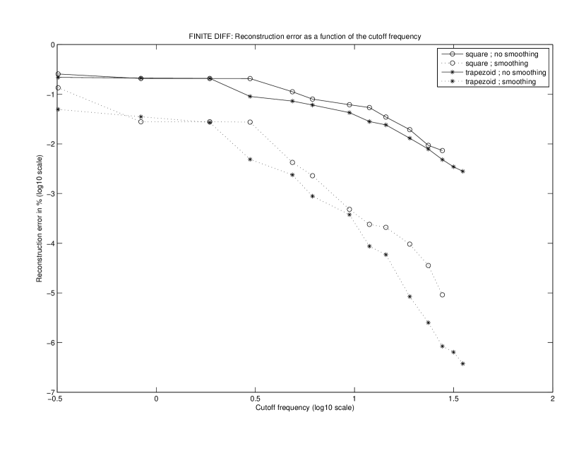
Refer to caption
Figure 27: Reconstruction errors for the finite differences and exact methods, as a function of the cutoff frequency (i.e., the largest eigenvalue used for the control computation), with or without time- and space-smoothing.
Refer to caption
Figure 28: Reconstruction errors for the finite differences method, in the square and in the trapezoid, as a function of the cutoff frequency (i.e., the largest eigenvalue used for the control computation), with or without time- and space-smoothing.

4.4 Energy of the control function

In this paragraph we investigate the impact of the smoothing, the width of the control domain U𝑈U and the control time T𝑇T on various outputs such as the condition number of MTsubscript𝑀𝑇M_{T}, the reconstruction error uynorm𝑢𝑦\|u-y\|, and the norm of the control function wnorm𝑤\|w\|.
To do so we performed several one-mode experiments (see paragraph 4.1, mode 500) in the square, with exact eigenvalues, 1000 eigenvalues used for computation of MTsubscript𝑀𝑇M_{T}, 2000 eigenvalues used for reconstruction and verification. We chose various times: 2.5 and 8, plus their “smoothed” counterparts, according to the empirical formula Tsmooth=15/8Tsubscript𝑇smooth158𝑇T_{\textrm{smooth}}=15/8*T. This increase of Tsmoothsubscript𝑇smoothT_{\textrm{smooth}} is justified on the theoretical level by formulas (31) and (30) which show that the efficiency of the control is related to a mean value of χ(t,x)𝜒𝑡𝑥\chi(t,x) on the trajectories. Similarly, we chose various width of U𝑈U: 1/10 and 3/10, plus their “smoothed” counterpart, which are double. Table 3 presents the numerical results for these experiments. This table draws several remarks. First, the condition number of MTsubscript𝑀𝑇M_{T}, the reconstruction error and the norm of the control w𝑤w decrease with increasing time and U𝑈U. Second, if we compare each non-smooth experiment with its “smoothed” counterpart (the comparison is of course approximate, since the “smoothed” time and width formulas are only reasonable approximations), the condition number seems similar, as well as the norm of the control function w𝑤w, whereas the reconstruction error is far smaller with smoothing than without.

Smooth Width of U𝑈U Time Condition number Rec. error wnorm𝑤\|w\|
no 1/10 2.5 48.8303 0.00518843 504.287
yes 2/10 2.5 204.048 0.00140275 1837.12
yes 2/10 4.7 21.7869 4.65892E-07 364.013
no 1/10 8 21.1003 0.00162583 120.744
yes 2/10 8 16.5497 8.51442E-08 189.361
yes 2/10 15 12.017 8.39923E-09 100.616
no 3/10 2.5 4.20741 0.0014823 147.009
yes 6/10 2.5 9.05136 1.94519E-06 336.704
yes 6/10 4.7 3.09927 2.99855E-08 125.481
no 3/10 8 3.20921 0.000488423 39.9988
yes 6/10 8 2.74172 6.0204E-09 69.8206
yes 6/10 15 2.4113 8.55119E-10 37.1463
Table 3: Impact of the control time, the width of U𝑈U and the smoothing, on the condition number of MTsubscript𝑀𝑇M_{T}, on the reconstruction error and on the norm of the control function. These results come from one-mode experiments in the square, with exact eigenvalues.

Figures 29 and 30 emphasize the impact of the control time, they present the reconstruction error, the norm of the control, and the condition number of MTsubscript𝑀𝑇M_{T}, as a function of the control time (varying between 2.5 and 16), with or without smoothing. Conclusions are similar to the table conclusions.

Refer to caption
Refer to caption
Figure 29: Experiments in the square, with exact eigenvalues: impact of the smoothing on the reconstruction error (top) and on the norm of the control function (bottom), as a function of the control time.
Refer to caption
Figure 30: Experiments in the square, with exact eigenvalues: impact of the smoothing on the condition number of the MTsubscript𝑀𝑇M_{T} matrix, as a function of the control time.

4.5 Condition number

In this section, we investigate conjecture 2. To do so, we compute the condition number of MT,ωsubscript𝑀𝑇𝜔M_{T,\omega}, as we have:

cond(MT,ω)=MT,ω.MT,ω1MT.MT,ω1formulae-sequencecondsubscript𝑀𝑇𝜔normsubscript𝑀𝑇𝜔similar-to-or-equalsnormsuperscriptsubscript𝑀𝑇𝜔1normsubscript𝑀𝑇normsuperscriptsubscript𝑀𝑇𝜔1\textrm{cond}(M_{T,\omega})=\|M_{T,\omega}\|.\|M_{T,\omega}^{-1}\|\simeq\|M_{T}\|.\|M_{T,\omega}^{-1}\| (75)

Figure 31 shows the condition number of the MTsubscript𝑀𝑇M_{T} matrix as a function of the control time or of the last eigenvalue used for the control function computation. According to conjecture 2, we obtain lines of the type

log(cond(MT,ω))=ω.C(T,U)formulae-sequencecondsubscript𝑀𝑇𝜔𝜔𝐶𝑇𝑈\log\left(\textrm{cond}(M_{T,\omega})\right)=\omega.C(T,U) (76)

Figure 32 shows for various eigenvalues numbers the following curves:

Tlog(cond(MT,ω))ωmaps-to𝑇condsubscript𝑀𝑇𝜔𝜔T\mapsto\frac{\log\left(\textrm{cond}(M_{T,\omega})\right)}{\omega} (77)

Similarly, we can draw conclusions compatible with conjecture 2, as these curves seems to converge when the number of eigenvalues grows to infinity.

Refer to caption
Figure 31: Condition number of the MT,ωsubscript𝑀𝑇𝜔M_{T,\omega} matrix as a function of the cutoff frequency ω𝜔\omega for various control times.
Refer to caption
Figure 32: Ratio of the log of the condition number of the MT,ωsubscript𝑀𝑇𝜔M_{T,\omega} matrix and the cutoff frequency ω𝜔\omega, as a function of the control time for various eigenvalues numbers.

4.6 Non-controlling domains

In this section we investigate two special experiments with non-controlling domains, i.e. such that the geometric control condition is not satisfied whatever the control time.
First we consider the domain presented in Figure 33.
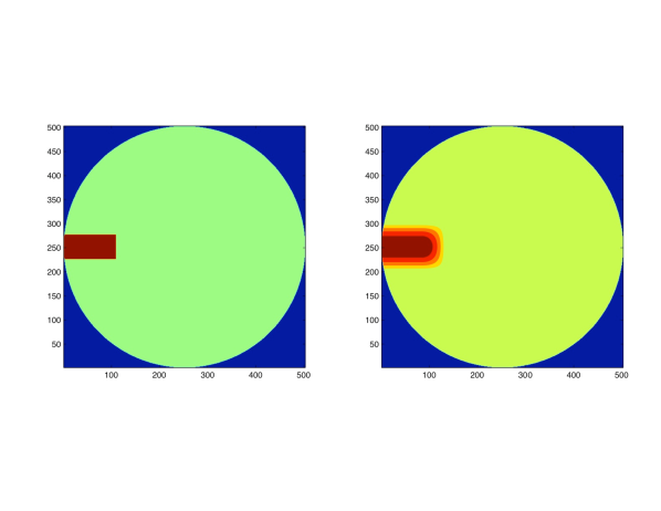
Refer to caption
Figure 33: Non-controlling domain U𝑈U without (left) or with (right) smoothing. This domain consists of the neighborhood of a radius which is truncated around the disc boundary.

For this domain the condition number of the MTsubscript𝑀𝑇M_{T} matrix is large, and subsequently we should be experiencing difficulties to reconstruct the data u𝑢u. We perform one-mode experiments with two different eigenvectors, one being localized in the center of the disc (eigenvalue 60), the other being localized around the boundary (eigenvalue 53) as can be seen on Figure 34.
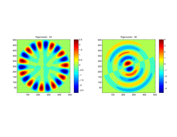
Refer to caption
Figure 34: Special modes chosen for experiment with non-controlling domains, corresponding to the 53rd and 60th eigenvalues.

The various outputs are presented in Table 4, and we can see that the inversion is fairly accurate for the 53rd eigenmode, while it is logically poor for the 60th eigenmode. Moreover, the energy needed for the control process, i.e. the norm of the control w𝑤w, is small for the 53rd eigenvector, while it is large for the 60-th. We can also notice that the smoothing has the noticeable effect to decrease the reconstruction error, the norm of the control function w𝑤w being similar.

Condition 53rd Eigenmode 60th Eigenmode
smooth? number Rec. error wnorm𝑤\|w\| Rec. error wnorm𝑤\|w\|
no 4960 0.63% 15 26% 4583
yes 6042 6.5 104superscript10410^{-4}% 24 0.11% 8872
Table 4: Influence of the shape of the data on the reconstruction error and the norm of the control, with a non-controlling domain U𝑈U. On the left, the 53rd eigenmode is localized around the boundary of the circle, as is the control domain. On the right, the 60th eigenmode is localized around the center of the circle.

In the second experiment we change the point of view: instead of considering one given domain and two different data, we consider one given data, and two different non-controlling domains. The data is again u53subscript𝑢53u_{53} (see Figure 34), which is localized at the boundary of the disc. The first domain is the previous one (see Figure 33), the second domain is presented in Figure 35, it is localized at the center of the disc.
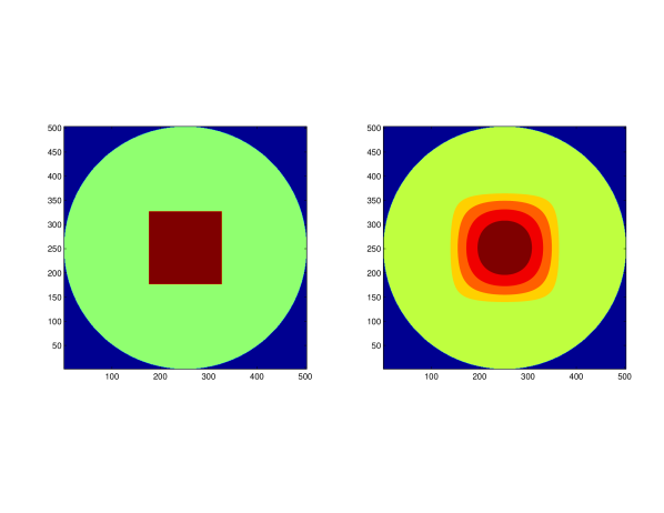
Refer to caption
Figure 35: Non-controlling domain U𝑈U without (left) or with (right) smoothing. This domain consists of the neighborhood of a radius which is truncated around the disc center.

In either case, the condition number of the MTsubscript𝑀𝑇M_{T} matrix is large, and the data should prove difficult to reconstruct. Table 5 present the outputs we get for the two domains. As previously, we observe that the control process works fairly well for the appropriate control domain, with a small error as well as a small energy for the control. Conversely, when the control domain does not “see” the input data, the results are poorer: the energy needed is large with or without smoothing, the error is also large without smoothing, it is however small with smoothing.

First domain Second domain
smooth? Cond. nb. Rec. error wnorm𝑤\|w\| Cond. nb. Rec. error wnorm𝑤\|w\|
no 4960 0.63% 15 3.6 106superscript10610^{6} 68% 1.9 104superscript10410^{4}
yes 6042 6.5 104superscript10410^{-4}% 24 3.3 105superscript10510^{5} 9.4 103superscript10310^{-3}% 6.5 105superscript10510^{5}
Table 5: Reconstruction error and the norm of the control with a data u53subscript𝑢53u_{53} localized at the boundary of the disc and two different non-controlling domains U𝑈U, the first one being localized around the boundary, the second one around the center.

Acknowledgement

The experiments have been realized with Matlab555The Mathworks, Inc. http://www.mathworks.fr software on Laboratoire Jean-Alexandre Dieudonné (Nice) and Laboratoire Jean Kuntzmann (Grenoble) computing machines. The INRIA Gforge666http://gforge.inria.fr has also been used. The authors thank J.-M. Lacroix (Laboratoire J.-A. Dieudonné) for his managing of Nice computing machine.
This work has been partially supported by Institut Universitaire de France.

References

  • [AL98] M. Asch and G. Lebeau. Geometrical aspects of exact boundary controllability of the wave equation. a numerical study. ESAIM:COCV, 3:163–212, 1998.
  • [BL01] N. Burq and G. Lebeau. Mesures de défaut de compacité, application au système de lamé. Ann. Sci. École Norm. Sup., 34(6):817–870, 2001.
  • [BLR92] C. Bardos, G. Lebeau, and J. Rauch. Sharp sufficient conditions for the observation, control and stabilisation of waves from the boundary. SIAM J.Control Optim., 305:1024–1065, 1992.
  • [DL09] B. Dehman and G. Lebeau. Analysis of the HUM Control Operator and Exact Controllability for Semilinear Waves in Uniform Time. to appear in SIAM Control and Optimization, 2009.
  • [Gér91] P. Gérard. Microlocal defect measures. C.P.D.E, 16:1762–1794, 1991.
  • [GHL08] R. Glowinski, J. W. He, and J.-L. Lions. Exact and Approximate Controllability for Distributed Parameter Systems: A Numerical Approach. Cambridge University Press, 2008.
  • [GLL90] R. Glowinski, C.H. Li, and J.L. Lions. A numerical approach to the exact boundary controllability of the wave equation (I). dirichlet controls : description of the numerical methods. Japan J. Appl. Math., 7:1–76, 1990.
  • [Hör85] L. Hörmander. The analysis of linear partial differential operators. III. Grundl. Math. Wiss. Band 274. Springer-Verlag, Berlin, 1985. Pseudodifferential operators.
  • [Leb92] G. Lebeau. Contrôle analytique I : Estimations a priori. Duke Math. J., 68(1):1–30, 1992.
  • [Lio88] J.-L. Lions. Contrôlabilité exacte, perturbations et stabilisation de systèmes distribués. Tome 2, volume 9 of Recherches en Mathématiques Appliquées [Research in Applied Mathematics]. Masson, Paris, 1988.
  • [MS78] R.-B. Melrose and J. Sjostrand. Singularities of boundary value problems I. CPAM, 31:593–617, 1978.
  • [MS82] R.-B. Melrose and J. Sjostrand. Singularities of boundary value problems II. CPAM, 35:129–168, 1982.
  • [Rus78] D.-L. Russell. Controllability and stabilizability theory for linear partial differential equations: recent progress and open questions. SIAM Rev, 20:639–739, 1978.
  • [Tay81] M. Taylor. Pseudodifferential operators. Princeton University Press, 1981.
  • [Zua02] E. Zuazua. Controllability of partial differential equations and its semi-discrete approximations. Discrete and Continuous Dynamical Systems, 8(2):469–513, 2002.
  • [Zua05] E. Zuazua. Propagation, observation, and control of waves approximated by finite difference methods. SIAM Rev, 47(2):197–243, 2005.