Abstract

The scattering amplitude for the longitudinal weak bosons is investigated in the $SU(3)$ gauge-Higgs unification as a function of the scattering energy, the Wilson line phase $\theta_{\rm H}$ and the warp factor. The $\theta_{\rm H}$-dependence of the amplitude is quite different in the flat and the warped spacetimes. Generically the amplitude is enhanced for $\theta_{\rm H}={\cal O}(1)$ in the warped case while it is almost independent of $\theta_{\rm H}$ in the flat case. This indicates the tree-level unitarity is violated in the warped case at a lower scale than that in the flat case.

OU-HET 627/2009

RIKEN-TH-153


Weak boson scattering in Gauge-Higgs Unification

Naoyuki Haba,${}^{1}\!$ 111e-mail address: haba@het.phys.sci.osaka-u.ac.jp Yutaka Sakamura${}^{2}\!$ 222e-mail address: sakamura@riken.jp and Toshifumi Yamashita${}^{3}\!$ 333e-mail address: yamasita@eken.phys.nagoya-u.ac.jp

1Department of Physics, Osaka University, Toyonaka, Osaka 560-0043, Japan

2RIKEN, Wako, Saitama 351-0198, Japan

3Department of Physics, Nagoya University, Nagoya 464-8602, Japan


1 Introduction

The origin of the electroweak symmetry breaking is still a mystery since the Higgs boson has not been discovered yet. Extra dimensions open up new possibility for it. For example, it can occur by nontrivial boundary conditions or the Wilson line phases along the extra dimensions, such as the Higgsless models [1] or the gauge-Higgs unification models [2]-[6]. Since these models are based on higher dimensional gauge theories and are thus nonrenormalizable, they should be interpreted as effective theories of more fundamental theories, which are valid below certain cutoff energy scales. This implies that the tree-level unitarity is violated at some scale, which is identified with the cutoff scale of the model. When we work in a higher dimensional theory, we have to know the cutoff scale of the theory in order to ensure the validity of the perturbative calculation.

The tree-level unitarity is usually discussed by evaluating the scattering amplitudes of the longitudinally polarized weak bosons $W^{\pm}_{L}$ and $Z_{L}$ at tree-level. In the standard model, the Higgs boson plays an important role for the recovery of the tree-level unitarity. If it is sufficiently heavy and decoupled, the scattering amplitudes for $W^{\pm}_{L}$ and $Z_{L}$ grow as $E^{2}$ where $E$ is the energy scale of the scattering, and exceed the unitarity bound at some scale around 1 TeV. This means that the perturbative calculation is no longer reliable above the scale. In the Higgsless models, the tree-level unitarity is recovered by the Kaluza-Klein (KK) modes of the gauge bosons [1] instead of the Higgs boson in the standard model, and the unitarity violation delays up to ${\cal O}(10~{}{\rm TeV})$ when the compactification scale is assumed to be around 1 TeV.

The situation is more complicated in the gauge-Higgs unification models because they have the Higgs mode (the fluctuation of the Wilson line phase $\theta_{\rm H}$) as well as the KK modes of the gauge bosons, both of which participate in the unitarization of the theory. In these models, both the coupling constants and the KK mass scale depend on $\theta_{\rm H}$ and thus the scattering amplitudes for $W^{\pm}_{L}$ and $Z_{L}$ have nontrivial $\theta_{\rm H}$-dependences. Especially the gauge-Higgs unification in the Randall-Sundrum warped spacetime [7]-[11] is interesting because the $WWH$ and the $ZZH$ couplings ($H$ stands for the Higgs mode) deviate from the standard model values and vanish for some specific values of $\theta_{\rm H}$, such as $\pi$ or $\pi/2$, depending on the models [10, 11]. For such values of $\theta_{\rm H}$, the Higgs mode cannot participate in the unitarization of the weak boson scattering. Therefore it is important to understand the $\theta_{\rm H}$-dependence of the scattering amplitudes for $W^{\pm}_{L}$ and $Z_{L}$ in order to estimate the cutoff scale of the models from the violation of the tree-level unitarity. This issue is discussed in Ref. [12] and some qualitative behaviors of the amplitude are clarified.

In this paper, we investigate various behaviors of the scattering amplitude more quantitatively by numerical calculations. We focus on the process: $W^{+}_{L}+W^{-}_{L}\to Z_{L}+Z_{L}$ in the gauge-Higgs unification model based on the five-dimensional (5D) $SU(3)$ gauge theory on $S^{1}/Z_{2}$ as the simplest example. Although this model gives the wrong value of the Weinberg angle $\theta_{W}$ and thus is not realistic, it has a lot of common features among the gauge-Higgs unification models. Hence it is a good starting point to understand the behaviors of the amplitudes peculiar to the gauge-Higgs unification. The Wilson line phase $\theta_{\rm H}$, which corresponds to the vacuum expectation value (VEV) of the Higgs field in the standard model, is dynamically determined at one-loop order if the whole matter content of the model is specified. In the following discussion, we do not specify the fermion sector and treat $\theta_{\rm H}$ as a free parameter because we are interested in the tree-level amplitude.

The paper is organized as follows. In Sec. 2, we briefly review the $SU(3)$ gauge-Higgs unification model and provide necessary ingredients to calculate the scattering amplitude for the weak bosons. In Sec. 3, we provide explicit expressions of the scattering amplitudes for the longitudinal weak bosons and for the (would-be) Nambu-Goldstone (NG) bosons, and show their behaviors as functions of $E$, $\theta_{\rm H}$ and the warp factor. Sec. 4 is devoted to the summary and discussions. In Appendix A, we give definitions and explicit forms of the basis functions used in the text. In Appendix B, we derive the 5D propagators of the gauge fields.

2 $SU(3)$ model

2.1 Set-up

We consider the 5D $SU(3)$ gauge theory compactified on $S^{1}/Z_{2}$ as the simplest example of the gauge-Higgs unification. Arbitrary background metric with 4D PoincarΓ© symmetry can be written as

$$ds^{2}=G_{MN}dx^{M}dx^{N}=e^{-2\sigma(y)}\eta_{\mu\nu}dx^{\mu}dx^{\nu}+dy^{2},$$ (2.1)

where $M,N=0,1,2,3,4$ are 5D indices and $\eta_{\mu\nu}={\rm diag}(-1,1,1,1)$. The fundamental region of $S^{1}/Z_{2}$ is $0\leq y\leq L$. The function $e^{\sigma(y)}$ is a warp factor, which is normalized as $\sigma(0)=0$. For example, $\sigma(y)=0$ in the flat spacetime, and $\sigma(y)=ky$ ($0\leq y\leq L$) in the Randall-Sundrum spacetime [13], where $k$ is the inverse AdS curvature radius.

The 5D gauge field $A_{M}$ is decomposed as

$$A_{M}=\sum_{\alpha=1}^{8}A_{M}^{\alpha}\frac{\lambda^{\alpha}}{2},$$ (2.2)

where $\lambda^{\alpha}$ are the Gell-Mann matrices. The 5D Lagrangian is

$\displaystyle{\cal L}\!\!\!$ $\displaystyle=\!\!\!$ $\displaystyle\sqrt{-G}\left[-{\rm tr}\left\{\frac{1}{2}G^{ML}G^{NP}F_{MN}F_{LP}+\frac{1}{\xi}\left(f_{\rm gf}\right)^{2}\right\}\right]+\cdots,$ (2.3)

where $\sqrt{-G}\equiv\sqrt{-\det(G_{MN})}=e^{-4\sigma}$, $F_{MN}\equiv\partial_{M}A_{N}-\partial_{N}A_{M}-ig_{5}\left[A_{M},A_{N}\right]$ ($g_{5}$ is the 5D gauge coupling), and $\xi$ is a dimensionless parameter. The ellipsis denotes the ghost and the matter sectors, which are irrelevant to the following discussion. The gauge-fixing function $f_{\rm gf}$ is chosen as

$\displaystyle f_{\rm gf}\!\!\!$ $\displaystyle=\!\!\!$ $\displaystyle e^{2\sigma}\left\{\eta^{\mu\nu}\partial_{\mu}A_{\nu}+\xi{\cal D}_{y}^{c}\left(e^{-2\sigma}A_{y}\right)\right\},$
$\displaystyle{\cal D}_{y}^{c}A_{M}\!\!\!$ $\displaystyle\equiv\!\!\!$ $\displaystyle\partial_{y}A_{M}-ig_{5}\left[A_{y}^{\rm bg},A_{M}\right],$ (2.4)

where $A_{y}^{\rm bg}(y)$ is the classical background of $A_{y}(x,y)$.

The boundary conditions for the gauge field is written as

$\displaystyle A_{\mu}(x,-y)\!\!\!$ $\displaystyle=\!\!\!$ $\displaystyle P_{0}A_{\mu}(x,y)P_{0}^{-1},\;\;\;A_{\mu}(x,L+y)=P_{L}A_{\mu}(x,L-y)P_{L}^{-1},$
$\displaystyle A_{y}(x,-y)\!\!\!$ $\displaystyle=\!\!\!$ $\displaystyle-P_{0}A_{y}(x,y)P_{0}^{-1},\;\;\;A_{y}(x,L+y)=-P_{L}A_{y}(x,L-y)P_{L}^{-1},$ (2.5)

where $P_{0}$ and $P_{L}$ are unitary matrices satisfying the relation $P_{0}^{2}=P_{L}^{2}=1$. By choosing them as $P_{0}=P_{L}={\rm diag}(-1,-1,1)$, the $Z_{2}$-parity eigenvalues $(P_{0},P_{L})$ of the gauge fields become

$\displaystyle A_{\mu}\!\!\!$ $\displaystyle=\!\!\!$ $\displaystyle\begin{pmatrix}(+,+)&(+,+)&(-,-)\\ (+,+)&(+,+)&(-,-)\\ (-,-)&(-,-)&(+,+)\end{pmatrix},\;\;\;\;\;A_{y}=\begin{pmatrix}(-,-)&(-,-)&(+,+)\\ (-,-)&(-,-)&(+,+)\\ (+,+)&(+,+)&(-,-)\end{pmatrix}.$ (2.6)

Note that only $(+,+)$ fields can have zero-modes when perturbation theory is developed around the trivial configuration $A_{M}=0$. Thus the $SU(3)$ gauge symmetry is broken to $SU(2)\times U(1)$ at tree-level. The zero-modes of $A_{y}$ form an $SU(2)$-doublet 4D scalar $(A_{y}^{4}+iA_{y}^{5},A_{y}^{6}+iA_{y}^{7})$, which plays a role of the Higgs doublet in the standard model whose VEV breaks $SU(2)\times U(1)$ to $U(1)_{\rm EM}$. They yield non-Abelian Aharonov-Bohm phases (Wilson line phases) when integrated along the fifth dimension. By using the residual $SU(2)\times U(1)$ symmetry, we can always push the nonvanishing VEV into $A_{y}^{7}$. Then the Wilson line phase $\theta_{\rm H}$ is given by

$$\theta_{\rm H}=g_{5}\int_{0}^{L}\!\!dy\;A_{y}^{\rm bg\,7}(y).$$ (2.7)

2.2 Mode expansion

The mode expansion of the 5D gauge fields is performed in a conventional way (see Ref. [8], for example). For the following discussion, it is convenient to move to the momentum representation for the 4D part while remain the coordinate representation for the fifth dimension. Then the 5D gauge fields are expanded into the KK modes as

$\displaystyle\tilde{A}_{\mu}^{\alpha}(p,y)\!\!\!$ $\displaystyle=\!\!\!$ $\displaystyle\sum_{n}u_{n}^{\alpha}(y)A_{\mu}^{(n)}(p)+\sum_{n}w_{n}^{\alpha}(y)p_{\mu}A_{\rm S}^{(n)}(p),$
$\displaystyle\tilde{A}_{y}^{\alpha}(p,y)\!\!\!$ $\displaystyle=\!\!\!$ $\displaystyle\sum_{n}v_{n}^{\alpha}(y)\varphi^{(n)}(p).$ (2.8)

Here we have moved to the Scherk-Schwarz basis, in which $\tilde{A}_{y}^{\rm bg}=0$. It is related to the original basis by the gauge transformation,

$$\tilde{A}_{M}=\Omega A_{M}\Omega^{-1}-\frac{i}{g_{5}}\left(\partial_{M}\Omega\right)\Omega^{-1},$$ (2.9)

with

$$\Omega(y)\equiv{\cal P}\exp\left\{-ig_{5}\int_{0}^{y}\!\!dy^{\prime}\;A_{y}^{\rm bg\,7}(y^{\prime})\cdot\frac{\lambda^{7}}{2}\right\}.$$ (2.10)

The symbol ${\cal P}$ stands for the path ordered operator from left to right. Notice that $\tilde{A}_{\mu}^{\alpha}(p,y)$ are decomposed into two parts, according to their polarization. In the above expression, $A_{\mu}^{(n)}(p)$ are polarized as $p^{\mu}A_{\mu}^{(n)}(p)=0$ and include the transverse and the longitudinal modes, which are physical for the massive modes. On the other hand, $A_{\rm S}^{(n)}(p)$ are unphysical scalar modes. The gauge-scalar modes $\varphi^{(n)}(p)$ are also unphysical besides the zero-mode.

The mode functions $w_{n}^{\alpha}(y)$ and $v_{n}^{\alpha}(y)$ are related to each other by

$\displaystyle v_{n}^{\alpha}(y)\!\!\!$ $\displaystyle=\!\!\!$ $\displaystyle\frac{d}{dy}w_{n}^{\alpha}(y),$
$\displaystyle w_{n}^{\alpha}(y)\!\!\!$ $\displaystyle=\!\!\!$ $\displaystyle-\frac{\xi}{\tilde{m}_{n}^{2}}\frac{d}{dy}\left\{e^{-2\sigma(y)}v_{n}^{\alpha}(y)\right\},$ (2.11)

where $\tilde{m}_{n}$ are common mass eigenvalues for $A_{\rm S}^{(n)}$ and $\varphi^{(n)}$. These relations hold irrespective of the value of the gauge parameter $\xi$. When $\xi=1$, they are further related to $u_{n}^{\alpha}(y)$ as

$$u_{n}^{\alpha}(y)=m_{n}w_{n}^{\alpha}(y),\;\;\;m_{n}=\tilde{m}_{n},$$ (2.12)

where $m_{n}$ are mass eigenvalues for $A_{\mu}^{(n)}$.

According to the transformation properties under the unbroken $U(1)_{\rm EM}$ symmetry and the rotation by a constant matrix $\Omega(L)$, the gauge fields are classified into the charged sector $(A_{M}^{1\pm i2},A_{M}^{4\pm i5})\equiv(A_{M}^{1}\pm iA_{M}^{2},A_{M}^{4}\pm iA_{M}^{5})/\sqrt{2}$ and the neutral sectors $(A_{M}^{3^{\prime}},A_{M}^{6})$, $A_{M}^{7}$ and $A_{M}^{8^{\prime}}$, where

$$\begin{pmatrix}A_{M}^{3^{\prime}}\\ A_{M}^{8^{\prime}}\end{pmatrix}\equiv\begin{pmatrix}-\frac{1}{2}&\frac{\sqrt{3}}{2}\\ -\frac{\sqrt{3}}{2}&-\frac{1}{2}\end{pmatrix}\begin{pmatrix}A_{M}^{3}\\ A_{M}^{8}\end{pmatrix}.$$ (2.13)

The $W$, $Z$ bosons and the photon are identified with the lowest modes in the $(A_{\mu}^{1\pm i2},A_{\mu}^{4\pm i5})$-, the $(A_{\mu}^{3^{\prime}},A_{\mu}^{6})$- and the $A_{\mu}^{8^{\prime}}$-sectors, respectively.

The mode functions for the $W$ boson are calculated as

$\displaystyle u_{W}^{1}(y)\!\!\!$ $\displaystyle\equiv\!\!\!$ $\displaystyle u_{0}^{1+i2}(y)=N_{W}c_{\theta}S_{0}(L,m_{W})C_{0}(y,m_{W}),$
$\displaystyle u_{W}^{4}(y)\!\!\!$ $\displaystyle\equiv\!\!\!$ u04+i​5​(y)=βˆ’NW​sθ​C0​(L,mW)​S0​(y,mW),superscriptsubscript𝑒04𝑖5𝑦subscriptπ‘π‘Šsubscriptπ‘ πœƒsubscript𝐢0𝐿subscriptπ‘šπ‘Šsubscript𝑆0𝑦subscriptπ‘šπ‘Š\displaystyle u_{0}^{4+i5}(y)=-N_{W}s_{\theta}C_{0}(L,m_{W})S_{0}(y,m_{W}), (2.14)

where $c_{\theta}\equiv\cos(\theta_{\rm H}/2)$, sθ≑sin⁑(ΞΈH/2)subscriptπ‘ πœƒsubscriptπœƒH2s_{\theta}\equiv\sin(\theta_{\rm H}/2), and $C_{0}(y,m)$, $S_{0}(y,m)$ are the basis functions defined in Appendix A. The mode functions for the $Z$ boson are

$\displaystyle u_{Z}^{3^{\prime}}(y)\!\!\!$ $\displaystyle\equiv\!\!\!$ $\displaystyle u_{0}^{3^{\prime}}(y)=N_{Z}\cos\theta_{\rm H}S_{0}(L,m_{Z})C_{0}(y,m_{Z}),$
$\displaystyle u_{Z}^{6}(y)\!\!\!$ $\displaystyle\equiv\!\!\!$ $\displaystyle u_{0}^{6}(y)=-N_{Z}\sin\theta_{\rm H}C_{0}(L,m_{Z})S_{0}(y,m_{Z}).$ (2.15)

Here the normalization constants $N_{W}$ and $N_{Z}$ are determined by

$$\int_{0}^{L}\!\!dy\;\left\{(u_{W}^{1})^{2}+(u_{W}^{4})^{2}\right\}=1,\;\;\;\;\;\int_{0}^{L}\!\!dy\;\left\{(u_{Z}^{3^{\prime}})^{2}+(u_{Z}^{6})^{2}\right\}=1,$$ (2.16)

and the $W$ and the $Z$ boson masses $m_{W}$ and $m_{Z}$ are the lowest solutions of

1mW​{C0′​(L,mW)​S0​(L,mW)+mW​eσ​(L)​sΞΈ2}1subscriptπ‘šπ‘Šsubscriptsuperscript𝐢′0𝐿subscriptπ‘šπ‘Šsubscript𝑆0𝐿subscriptπ‘šπ‘Šsubscriptπ‘šπ‘Šsuperscriptπ‘’πœŽπΏsuperscriptsubscriptπ‘ πœƒ2\displaystyle\frac{1}{m_{W}}\left\{C^{\prime}_{0}(L,m_{W})S_{0}(L,m_{W})+m_{W}e^{\sigma(L)}s_{\theta}^{2}\right\}\!\!\! $\displaystyle=\!\!\!$ $\displaystyle 0,$
$\displaystyle\frac{1}{m_{Z}}\left\{C^{\prime}_{0}(L,m_{Z})S_{0}(L,m_{Z})+m_{Z}e^{\sigma(L)}\sin^{2}\theta_{\rm H}\right\}\!\!\!$ $\displaystyle=\!\!\!$ $\displaystyle 0,$ (2.17)

respectively. The prime denotes the derivative for $y$. In the flat spacetime, for example, they are written for $0<\theta_{\rm H}<\pi$ as

$$m_{W}=\frac{\theta_{\rm H}}{2L},\;\;\;\;\;m_{Z}=\frac{\left|\pi-\left|\pi-2\theta_{\rm H}\right|\right|}{2L}.$$ (2.18)

For the corresponding gauge-scalar modes, the mode functions $v_{W}^{1,4}(y)$, $v_{Z}^{3^{\prime},6}(y)$ and their masses are obtained similarly.

2.3 5D propagators

For the purpose of calculating the scattering amplitude, it is convenient to use the 5D propagators defined in a mixed momentum/position representation [14]. It describes the propagation of the entire KK tower of excitations carrying the 4D momentum $p$ between two points $y$ and $y^{\prime}$ in the extra dimension. This approach has an advantage that we need not explicitly calculate the mass eigenvalues for the modes propagating in the internal lines of the Feynmann diagrams nor sum over contributions from the infinite number of KK modes.111 This approach is also useful for models with continuum spectra [15]. The explicit forms of the 5D propagators can be obtained by using the formula (B.10). For the charged sector $(A_{\mu}^{1+i2},A_{\mu}^{4+i5})$, the 5D propagator is calculated as

$\displaystyle G_{\rm T<}(y,y^{\prime})\!\!\!$ $\displaystyle=\!\!\!$ $\displaystyle\frac{e^{2\sigma(L)}}{\det_{(1,4)}{\cal W}}\begin{pmatrix}\left|p\right|e^{\sigma(L)}C_{0}(y)S_{0}(L)C_{L}(y^{\prime})&\\ &-S_{0}(y)C^{\prime}_{0}(L)S_{L}(y^{\prime})\end{pmatrix}$
βˆ’sθ​|p|​e3​σ​(L)det(1,4)𝒲​(sθ​C0​(y)​S0​(yβ€²)cθ​C0​(y)​S0​(yβ€²)cθ​S0​(y)​C0​(yβ€²)βˆ’sθ​S0​(y)​C0​(yβ€²)),subscriptπ‘ πœƒπ‘superscript𝑒3𝜎𝐿subscript14𝒲matrixsubscriptπ‘ πœƒsubscript𝐢0𝑦subscript𝑆0superscript𝑦′subscriptπ‘πœƒsubscript𝐢0𝑦subscript𝑆0superscript𝑦′subscriptπ‘πœƒsubscript𝑆0𝑦subscript𝐢0superscript𝑦′subscriptπ‘ πœƒsubscript𝑆0𝑦subscript𝐢0superscript𝑦′\displaystyle-\frac{s_{\theta}\left|p\right|e^{3\sigma(L)}}{\det_{(1,4)}{\cal W}}\begin{pmatrix}s_{\theta}C_{0}(y)S_{0}(y^{\prime})&c_{\theta}C_{0}(y)S_{0}(y^{\prime})\\ c_{\theta}S_{0}(y)C_{0}(y^{\prime})&-s_{\theta}S_{0}(y)C_{0}(y^{\prime})\end{pmatrix},
$\displaystyle G_{\rm T>}(y,y^{\prime})\!\!\!$ $\displaystyle=\!\!\!$ $\displaystyle\left\{G_{\rm T<}(y^{\prime},y)\right\}^{t},$ (2.19)

where $\left|p\right|\equiv\sqrt{-p^{2}}$, and $\det_{(1,4)}$ is the determinant of ${\cal W}$ defined in (B.11) restricted to the $(A_{\mu}^{1+i2},A_{\mu}^{4+i5})$-sector and

$\displaystyle{\rm det}_{(1,4)}{\cal W}\!\!\!$ $\displaystyle=\!\!\!$ βˆ’|p|​eσ​(L)​{C0′​(L)​S0​(L)+|p|eσ​(L)​sΞΈ2}.𝑝superscriptπ‘’πœŽπΏconditional-setlimit-fromsubscriptsuperscript𝐢′0𝐿subscript𝑆0𝐿conditional𝑝superscriptπ‘’πœŽπΏsuperscriptsubscriptπ‘ πœƒ2\displaystyle-\left|p\right|e^{\sigma(L)}\left\{C^{\prime}_{0}(L)S_{0}(L)+\left|p\right|e^{\sigma(L)}s_{\theta}^{2}\right\}. (2.20)

In the above expressions, we have omitted $\left|p\right|$ from the arguments. For the $(A_{\mu}^{3^{\prime}},A_{\mu}^{6})$-sector, the propagator is obtained from the above expressions by replacing $\theta_{\rm H}/2$ with $\theta_{\rm H}$. The propagators in the other sectors are calculated as

$\displaystyle G_{\rm T<}^{77}(y,y^{\prime},\left|p\right|)\!\!\!$ $\displaystyle=\!\!\!$ $\displaystyle e^{\sigma(L)}\frac{S_{0}(y,\left|p\right|)S_{L}(y^{\prime},\left|p\right|)}{\left|p\right|S_{0}(L,\left|p\right|)},$
$\displaystyle G_{\rm T<}^{8^{\prime}8^{\prime}}(y,y^{\prime},\left|p\right|)\!\!\!$ $\displaystyle=\!\!\!$ $\displaystyle-e^{2\sigma(L)}\frac{C_{0}(y,\left|p\right|)C_{L}(y^{\prime},\left|p\right|)}{C^{\prime}_{0}(L,\left|p\right|)}.$ (2.21)

3 Weak boson scattering

Now we consider the scattering of the weak bosons. The two-body scattering amplitudes are functions of the total energy $E$ and the scattering angle $\phi$ in the center-of-mass frame. For the elastic scattering of the $W$ bosons, there is an infrared singularity at $\phi=0$ due to the $t$-channel diagram exchanging the massless photon. Although such a singularity will be cancelled when the soft-photon emissions and higher loop corrections are taken into account, it involves some technical difficulties to obtain a finite value of the amplitude for the forward scattering. In order to avoid such difficulties, we consider the scattering process: $W_{L}^{+}(p_{1})+W_{L}^{-}(p_{2})\to Z_{L}(p_{3})+Z_{L}(p_{4})$ in the following. The subscript $L$ denotes the longitudinal polarization.

3.1 Scattering amplitude

As mentioned in Sec. 2.3, the scattering amplitudes are easily calculated by utilizing the 5D propagators. The scattering amplitude ${\cal A}$ is expressed by

$${\cal A}={\cal A}^{\rm C}+{\cal A}^{\rm V}+{\cal A}^{\rm S},$$ (3.1)

where ${\cal A}^{\rm C}$, ${\cal A}^{\rm V}$ and ${\cal A}^{\rm S}$ are contributions from the contact interaction, the exchange of the vector modes and that of the gauge-scalar modes, respectively. They are given by

$\displaystyle{\cal A}^{\rm C}\!\!\!$ $\displaystyle=\!\!\!$ $\displaystyle-\frac{ig_{5}^{2}}{4}\int_{0}^{L}\!\!dy\;\left\{(u_{W}^{1})^{2}+(u_{W}^{4})^{2}\right\}\left\{(u_{Z}^{3^{\prime}})^{2}+(u_{Z}^{6})^{2}\right\}$ (3.2)
$\displaystyle\times\left\{2(\varepsilon_{1}\cdot\varepsilon_{2})(\varepsilon_{3}^{*}\cdot\varepsilon_{4}^{*})-(\varepsilon_{1}\cdot\varepsilon_{3}^{*})(\varepsilon_{2}\cdot\varepsilon_{4}^{*})-(\varepsilon_{1}\cdot\varepsilon_{4}^{*})(\varepsilon_{2}\cdot\varepsilon_{3}^{*})\right\},$
$\displaystyle{\cal A}^{\rm V}\!\!\!$ $\displaystyle=\!\!\!$ $\displaystyle ig_{5}^{2}\sum_{\alpha,\beta=1,4}\int_{0}^{L}\!\!dy\int_{0}^{L}\!\!dy^{\prime}\;U_{WZ}^{\alpha}(y)G_{\rm T}^{\alpha\beta}(y,y^{\prime},\left|p_{13}\right|)U_{WZ}^{\beta}(y^{\prime})P_{1324}$ (3.3)
$\displaystyle+ig_{5}^{2}\sum_{\alpha,\beta=1,4}\int_{0}^{L}\!\!dy\int_{0}^{L}\!\!dy^{\prime}\;U_{WZ}^{\alpha}(y)G_{\rm T}^{\alpha\beta}(y,y^{\prime},\left|p_{14}\right|)U_{WZ}^{\beta}(y^{\prime})P_{1423},$
$\displaystyle{\cal A}^{\rm S}\!\!\!$ $\displaystyle=\!\!\!$ $\displaystyle ig_{5}^{2}\int_{0}^{L}\!\!dy\;Y_{WW}^{7}(y)Y_{ZZ}^{7}(y)\frac{(\varepsilon_{1}\cdot\varepsilon_{2})(\varepsilon_{3}^{*}\cdot\varepsilon_{4}^{*})}{p_{12}^{2}}$ (3.4)
$\displaystyle+ig_{5}^{2}\sum_{\alpha=1,4}\int_{0}^{L}\!\!dy\;Y_{WZ}^{\alpha}(y)Y_{WZ}^{\alpha}(y)\left\{\frac{(\varepsilon_{1}\cdot\varepsilon_{3}^{*})(\varepsilon_{2}\cdot\varepsilon_{4}^{*})}{p_{13}^{2}}+\frac{(\varepsilon_{1}\cdot\varepsilon_{4}^{*})(\varepsilon_{2}\cdot\varepsilon_{3}^{*})}{p_{14}^{2}}\right\},$

where $\varepsilon_{i}$ ($i=1,2,3,4$) are the polarization vectors, $p_{12}\equiv p_{1}+p_{2}$, $p_{13}\equiv p_{1}-p_{3}$, $p_{14}\equiv p_{1}-p_{4}$,

$\displaystyle P_{1324}\!\!\!$ $\displaystyle\equiv\!\!\!$ $\displaystyle\left\{2(p_{1}\cdot\varepsilon_{3}^{*})\varepsilon_{1}+2(p_{3}\cdot\varepsilon_{1})\varepsilon_{3}^{*}-(\varepsilon_{1}\cdot\varepsilon_{3}^{*})(p_{1}+p_{3})\right\}^{\mu}\left(\eta_{\mu\nu}-\frac{p_{13\mu}p_{13\nu}}{p_{13}^{2}}\right)$
$\displaystyle\times\left\{2(p_{2}\cdot\varepsilon_{4}^{*})\varepsilon_{2}+2(p_{4}\cdot\varepsilon_{2})\varepsilon_{4}^{*}-(\varepsilon_{2}\cdot\varepsilon_{4}^{*})(p_{2}+p_{4})\right\}^{\nu},$
$\displaystyle P_{1423}\!\!\!$ $\displaystyle\equiv\!\!\!$ $\displaystyle\left\{2(p_{1}\cdot\varepsilon_{4}^{*})\varepsilon_{1}+2(p_{4}\cdot\varepsilon_{1})\varepsilon_{4}^{*}-(\varepsilon_{1}\cdot\varepsilon_{4}^{*})(p_{1}+p_{4})\right\}^{\mu}\left(\eta_{\mu\nu}-\frac{p_{14\mu}p_{14\nu}}{p_{14}^{2}}\right)$ (3.5)
$\displaystyle\times\left\{2(p_{2}\cdot\varepsilon_{3}^{*})\varepsilon_{2}+2(p_{3}\cdot\varepsilon_{2})\varepsilon_{3}^{*}-(\varepsilon_{2}\cdot\varepsilon_{3}^{*})(p_{2}+p_{3})\right\}^{\nu},$

and the functions in the integrands are defined as

$\displaystyle U_{WZ}^{1}\!\!\!$ $\displaystyle=\!\!\!$ $\displaystyle\frac{1}{2}\left(u_{W}^{1}u_{Z}^{3^{\prime}}+u_{W}^{4}u_{Z}^{6}\right),\;\;\;\;\;U_{WZ}^{4}=\frac{1}{2}\left(u_{W}^{1}u_{Z}^{6}-u_{W}^{4}u_{Z}^{3^{\prime}}\right),$
$\displaystyle Y_{WW}^{7}\!\!\!$ $\displaystyle=\!\!\!$ $\displaystyle e^{-2\sigma}\left\{(u_{W}^{1})^{\prime}u_{W}^{4}-u_{W}^{1}(u_{W}^{4})^{\prime}\right\},\;\;\;\;\;Y_{ZZ}^{7}=2e^{-2\sigma}\left\{(u_{Z}^{3^{\prime}})^{\prime}u_{Z}^{6}-u_{Z}^{3^{\prime}}(u_{Z}^{6})^{\prime}\right\},$
$\displaystyle Y_{WZ}^{1}\!\!\!$ $\displaystyle=\!\!\!$ $\displaystyle\frac{e^{-2\sigma}}{2}\left\{(u_{W}^{1})^{\prime}u_{Z}^{3^{\prime}}-u_{W}^{1}(u_{Z}^{3^{\prime}})^{\prime}+(u_{W}^{4})^{\prime}u_{Z}^{6}-u_{W}^{4}(u_{Z}^{6})^{\prime}\right\},$
$\displaystyle Y_{WZ}^{4}\!\!\!$ $\displaystyle=\!\!\!$ $\displaystyle\frac{e^{-2\sigma}}{2}\left\{(u_{W}^{1})^{\prime}u_{Z}^{6}-u_{W}^{1}(u_{Z}^{6})^{\prime}-(u_{W}^{4})^{\prime}u_{Z}^{3^{\prime}}+u_{W}^{4}(u_{Z}^{3^{\prime}})^{\prime}\right\}.$ (3.6)

Here we have used the relation $p_{i}\cdot\varepsilon_{i}(p_{i})=0$ ($i=1,2,3,4$).

The first and the second lines in (3.3) correspond to the $t$-channel and the $u$-channel diagrams exchanging the $W$ boson and its KK modes, respectively. The above expression of the amplitude is a result of a cancellation between the gauge-dependent part $G_{\rm S}(y,y^{\prime},\left|p\right|)$ in the propagator of the vector modes and the gauge-scalar propagator $G_{yy}(y,y^{\prime},\left|p\right|)$. This cancellation occurs due to the relation (B.16) and makes the resultant amplitude gauge-independent. The contribution ${\cal A}^{\rm S}$ is a remnant of the cancellation. The first line in (3.4) corresponds to the $s$-channel diagram exchanging the neutral gauge-scalar mode (i.e., the Higgs boson) while the second line represents the contributions from the $t$-channel and the $u$-channel exchanges of the charged gauge-scalar modes. Notice that the Higgs boson is massless at tree-level in the gauge-Higgs unification. It acquires a nonzero mass at one-loop order.

The gauge invariance of the theory ensures the equivalence theorem [16], which states that the scattering of the longitudinally polarized vector bosons is equivalent to that of the (would-be) NG bosons eaten by the gauge bosons. In 5D models, the gauge-scalar modes $\varphi^{(n)}$ coming from $A_{y}$ play the role of the NG bosons in the equivalence theorem [1, 17].222 When there exist additional bulk Higgs fields that break the gauge symmetry, the NG bosons become mixture of modes from the bulk Higgs fields and $A_{y}$. Namely, the following relation holds for the longitudinal vector modes $A_{L}^{(n)}$.

$$T(A_{L}^{(n_{1})},\cdots,A_{L}^{(n_{l})};\Phi)=C_{l}T(i\varphi^{(n_{1})},\cdots,i\varphi^{(n_{l})};\Phi)+{\cal O}\left(\frac{M^{2}}{E^{2}}\right),$$ (3.7)

where all external lines are directed inwards, $\Phi$ denotes any possible amputated external physical fields, such as the transverse gauge boson, and $M$ is the heaviest mass among the external lines. A constant $C_{l}$ is gauge-dependent, but $C_{l}=1$ at tree-level.333 We can also take a gauge where $C_{l}=1$ at all orders of the perturbative expansion [18]. The correction term is ${\cal O}(M^{2}/E^{2})$ because of the 5D gauge invariance (see Ref. [19], for example). Eq.(3.7) is useful to discuss the high-energy behavior of the scattering amplitude ${\cal A}$ because the corresponding NG boson amplitude does not have ${\cal O}(E^{4})$ contributions,444 For the non-forward (non-backward) scattering, ${\cal O}(E^{2})$ contributions are also absent. which makes it easier to numerically calculate the amplitude thanks to the absence of cancellations between large numbers.

The scattering amplitude for the corresponding NG bosons comes only from the diagrams exchanging the vector modes.

$\displaystyle{\cal B}\!\!\!$ $\displaystyle=\!\!\!$ $\displaystyle ig_{5}^{2}\sum_{\alpha,\beta=1,4}\int_{0}^{L}\!\!dy\int_{0}^{L}\!\!dy^{\prime}\;V_{WZ}^{\alpha}(y)(p_{1}+p_{3})^{\mu}G_{\mu\nu}^{\alpha\beta}(p_{13},y,y^{\prime})(p_{2}+p_{4})^{\nu}V_{WZ}^{\beta}(y^{\prime})$ (3.8)
$\displaystyle+ig_{5}^{2}\sum_{\alpha,\beta=1,4}\int_{0}^{L}\!\!dy\int_{0}^{L}\!\!dy^{\prime}\;V_{WZ}^{\alpha}(y)(p_{1}+p_{4})^{\mu}G_{\mu\nu}^{\alpha\beta}(p_{14},y,y^{\prime})(p_{2}+p_{3})^{\nu}V_{WZ}^{\beta}(y^{\prime}),$

where

$\displaystyle V_{WZ}^{1}\!\!\!$ $\displaystyle\equiv\!\!\!$ $\displaystyle\frac{e^{-2\sigma}}{2}\left(v_{W}^{1}v_{Z}^{3^{\prime}}+v_{W}^{4}v_{Z}^{6}\right),$
$\displaystyle V_{WZ}^{4}\!\!\!$ $\displaystyle\equiv\!\!\!$ $\displaystyle\frac{e^{-2\sigma}}{2}\left(v_{W}^{1}z_{Z}^{6}-v_{W}^{4}v_{Z}^{3^{\prime}}\right).$ (3.9)

3.2 Various behaviors of the amplitudes

Here we show various behaviors of the scattering amplitudes given in the previous subsection. For the numerical calculation, we choose the gauge parameter as $\xi=1$, the 4D gauge coupling $g_{4}\equiv g_{5}/\sqrt{L}$ as $g_{4}^{2}=0.1$, and take the $W$ boson mass $m_{W}$ as an input parameter. Then the size of the extra dimension $L$ becomes $\theta_{\rm H}$-dependent after fixing $m_{W}$. (See Eq.(2.18), for example.) The KK mass scale $m_{\rm KK}\equiv\pi k/(e^{kL}-1)$ is also $\theta_{\rm H}$-dependent. Thus the amplitudes are functions of the center-of-mass energy $E$, the Wilson line phase $\theta_{\rm H}$ and the warp factor $e^{kL}$. The physical amplitude ${\cal A}$ is of course gauge-independent, and the $\xi$-dependence of the NG boson amplitude ${\cal B}$ is small in high-energy region as can be seen from (3.7). The 4 momenta and the polarization vectors of the initial and final states are parameterized as in Table. I. There, $p_{W}\equiv\sqrt{E^{2}/4-m_{W}^{2}}$, $p_{Z}\equiv\sqrt{E^{2}/4-m_{Z}^{2}}$, and $\phi$ is the scattering angle in the center-of-mass frame. Notice that the amplitudes ${\cal A}$ in (3.1) and ${\cal B}$ in (3.8) are symmetric under $\phi\leftrightarrow\pi-\phi$.

$p_{1}=(E/2,0,0,p_{W})$ $\varepsilon_{1}(p_{1})=(p_{W},0,0,E/2)/m_{W}$
$p_{2}=(E/2,0,0,-p_{W})$ $\varepsilon_{2}(p_{2})=(p_{W},0,0,-E/2)/m_{W}$
$p_{3}=(E/2,p_{Z}\sin\phi,0,p_{Z}\cos\phi)$ $\varepsilon_{3}(p_{3})=(p_{Z},(E/2)\sin\phi,0,(E/2)\cos\phi)/m_{Z}$
$p_{4}=(E/2,-p_{Z}\sin\phi,0,-p_{Z}\cos\phi)$ $\varepsilon_{4}(p_{4})=(p_{Z},-(E/2)\sin\phi,0,-(E/2)\cos\phi)/m_{Z}$
Table I: The 4 momenta and the polarization vectors of the initial and the final states for $W_{L}^{+}(p_{1})+W_{L}^{-}(p_{2})\to Z_{L}(p_{3})+Z_{L}(p_{4})$. $E$ is the center-of-mass energy, $p_{W}\equiv\sqrt{E^{2}/4-m_{W}^{2}}$, $p_{Z}\equiv\sqrt{E^{2}/4-m_{Z}^{2}}$, and $\phi$ is the scattering angle in the center-of-mass frame.

3.2.1 Non-forward scattering

Refer to caption
Refer to caption
Figure 1: The energy dependence of the amplitudes for $W^{+}_{L}+W^{-}_{L}\to Z_{L}+Z_{L}$. The solid lines represent the vector boson scattering ${\cal A}$, and the dashed lines are the NG boson scattering ${\cal B}$. The scattering angle is chosen as $\phi=\pi/3$. In the flat case (the left figure), the amplitudes are independent of the Wilson line phase $\theta_{\rm H}$ for $0<\theta_{\rm H}<\pi/2$.

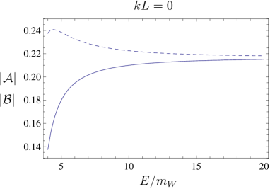
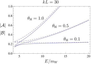
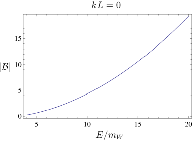
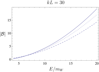
First we consider a non-forward (and non-backward) scattering. We choose the scattering angle as $\phi=\pi/3$ in the following. Fig. 1 shows the energy dependence of the scattering amplitudes. The solid and the dashed lines represent the scattering amplitudes for the vector bosons ${\cal A}$ and for the NG bosons ${\cal B}$, respectively. We can explicitly see that the equivalence theorem holds both in the flat and the warped cases, and $\left|{\cal B}\right|-\left|{\cal A}\right|={\cal O}(m_{W}^{2}/E^{2})$.

In the flat case ($kL=0$), the amplitude ${\cal A}$ is independent of the Wilson line phase $\theta_{\rm H}$ in the range of $0<\theta_{\rm H}<\pi/2$. It approaches to a constant value at high energies. In the case of the warped geometry, on the other hand, The amplitude has a large $\theta_{\rm H}$-dependence and increase as $E^{2}$. It grows faster for larger $\theta_{\rm H}$.

These behaviors reflect the $\theta_{\rm H}$-dependences of the coupling constants among the gauge and the Higgs modes and of the KK mass scale $m_{\rm KK}$. Before explaining the behaviors of the amplitude, let us see the energy dependence of ${\cal B}$ again by rescaling the unit of the horizontal axes to $m_{\rm KK}$. (Fig. 2)

Refer to caption
Refer to caption
Figure 2: The energy dependence of the amplitude in the unit of $m_{\rm KK}$. The solid, dotted, dashed lines correspond to $\theta_{\rm H}=0.1,1.0,1.5$, respectively.

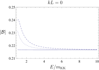
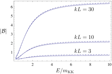
Then we can see that the amplitude approaches to constant values at sufficiently high energies even in the warped case. The constant values vary depending on the warp factor, and are larger than the value in the flat case by a factor $kL$ for $kL\stackrel{{\scriptstyle>}}{{{}_{\sim}}}{\cal O}(1)$. The $\theta_{\rm H}$-dependence we have seen in the right plot of Fig. 1 now almost disappears in the unit of $m_{\rm KK}$. It is cancelled by the $\theta_{\rm H}$-dependence of $m_{\rm KK}$ (see the beginning of Sec. 3.2.). The apparent $\theta_{\rm H}$-dependence of the plots in the flat case stems from the $\theta_{\rm H}$-dependence of $m_{\rm KK}$.

Now we will interpret the above behaviors of the amplitude. First of all, we should notice that the model reduces to the β€œstandard model” (SM), in which the Weinberg angle is $\sin^{2}\theta_{W}=3/4$ and the Higgs boson is massless, when $\theta_{\rm H}\ll 1$ irrespective of the 5D geometry. Every coupling constant in the gauge-Higgs sector takes almost the SM value and the KK modes are heavy enough to decouple. Thus the amplitude takes the same value as SM up to the energy scale where the KK modes start to propagate, i.e., $m_{\rm KK}$. The amplitude takes an almost constant value at $E\stackrel{{\scriptstyle>}}{{{}_{\sim}}}{\cal O}(10m_{W})$ in this case.

When $\theta_{\rm H}$ is not small, the coupling constants relevant to the amplitude deviate from the SM value. In the warped case, the $WWH$ and the $ZZH$ couplings become smaller than the SM values by $\cos(\theta_{\rm H}/2)$ and $\cos\theta_{\rm H}$ respectively, while the $WWZZ$ and the $WWZ$ couplings are almost unchanged [10, 11]. Thus ${\cal O}(E^{2})$ contributions miss to be cancelled among the low-lying modes and the amplitude grows in the low-energy region. For larger value of $\theta_{\rm H}$ (up to $\pi/2$), the deviation of the couplings are larger and then the amplitude grows faster. (See the right figure of Fig. 1.) This remaining ${\cal O}(E^{2})$ contribution is eventually cancelled by contributions from the KK modes. Namely, the amplitude ceases to increase and approaches to a constant value when the KK modes start to propagate.

The flat spacetime is a special case. As we mentioned, the amplitude becomes almost constant at $E\stackrel{{\scriptstyle>}}{{{}_{\sim}}}{\cal O}(10m_{W})$ when $\theta_{\rm H}\ll 1$. For larger values of $\theta_{\rm H}$, the $WWZZ$ and the $WWZ$ couplings slightly deviate from the SM values because of the nontrivial $y$-dependences of the mode functions for the $W$ and the $Z$ bosons [11], while the $WWH$ and the $ZZH$ couplings are now unchanged. Then the ${\cal O}(E^{2})$ contributions fail to be cancelled among the low-lying modes, just like in the warped case. However the contribution from the KK-modes completely cancel this ${\cal O}(E^{2})$, and the amplitude results in unchanged from the $\theta_{\rm H}\ll 1$ case. Namely the effect of the $\theta_{\rm H}$-dependence of the $WWZZ$ and $WWZ$ couplings and that of the KK mass spectrum are completely cancelled and the amplitude becomes $\theta_{\rm H}$-independent for $0<\theta_{\rm H}\leq\pi/2$ in the flat case. In the range of $\pi/2<\theta_{\rm H}<\pi$, the amplitude has a nontrivial $\theta_{\rm H}$-dependence. This stems from the fact that the relation $m_{Z}/m_{W}=2$ no longer holds (see Eq.(2.18)) and $m_{Z}$ also has a nontrivial $\theta_{\rm H}$-dependence in this region.

3.2.2 Forward scattering

Next we consider the forward scattering, i.e., $\phi=0$. In this case, an ${\cal O}(E^{2})$ contribution remains and the amplitude monotonically increases even above $m_{\rm KK}$. This is because the power counting of $E$ for the amplitude changes around $\phi=0$. For example, the brace part in (3.4) is expanded (for nonzero $\sin\phi$) as

$\displaystyle A_{tu}\!\!\!$ $\displaystyle\equiv\!\!\!$ $\displaystyle\frac{(\varepsilon_{1}\cdot\varepsilon_{3}^{*})(\varepsilon_{2}\cdot\varepsilon_{4}^{*})}{p_{13}^{2}}+\frac{(\varepsilon_{1}\cdot\varepsilon_{4}^{*})(\varepsilon_{2}\cdot\varepsilon_{3}^{*})}{p_{14}^{2}}$ (3.10)
$\displaystyle=\!\!\!$ $\displaystyle\frac{E^{2}}{4m_{W}^{2}m_{Z}^{2}}-\frac{m_{W}^{2}+m_{Z}^{2}}{2m_{W}^{2}m_{Z}^{2}}+\frac{2m_{W}^{2}m_{Z}^{2}+(m_{W}^{4}+m_{Z}^{4})\cos(2\phi)}{m_{W}^{2}m_{Z}^{2}E^{2}\sin^{2}\phi}+{\cal O}(E^{-4}).$

This means that the expansion becomes invalid when $\sin\phi\stackrel{{\scriptstyle<}}{{{}_{\sim}}}{\cal O}(m_{W}/E)$. At $\phi=0$, this quantity reduces to

$\displaystyle A_{tu}\!\!\!$ $\displaystyle=\!\!\!$ $\displaystyle\frac{(m_{W}^{4}+m_{Z}^{4})E^{2}}{2m_{W}^{2}m_{Z}^{2}(m_{Z}^{2}-m_{W}^{2})^{2}}-\frac{2(m_{W}^{2}+m_{Z}^{2})}{(m_{Z}^{2}-m_{W}^{2})^{2}},$ (3.11)

and the leading term for the high energy expansion changes. Therefore an ${\cal O}(E^{2})$ contribution is left in the total amplitude. Similar behavior of the amplitude is observed also in the standard model. Fig. 3 shows the energy dependence of the forward scattering amplitude. We can see that the amplitude grows as $E^{2}$ in any cases.

Refer to caption
Refer to caption
Figure 3: The energy dependence of the amplitude at $\phi=0$. The solid, dotted, dashed lines correspond to $\theta_{\rm H}=0.1,1.0,1.5$, respectively.

In the flat case, the amplitude does not have the $\theta_{\rm H}$-dependence again. In the warped case, it varies for different values of $\theta_{\rm H}$. For small values of $\theta_{\rm H}$, the amplitude has little dependence on the warp factor and takes almost the same value as the flat case. For larger values of $\theta_{\rm H}$, it becomes smaller in contrast to the non-forward scattering.

3.2.3 S-wave amplitude

The conventional bound for the tree-level unitarity is given by555 More restrictive unitarity condition is proposed in Ref. [20].

$$\left|a_{0}\right|\leq 1,$$ (3.12)

where $a_{0}$ is the s-wave amplitude defined as

$\displaystyle a_{0}(E)\!\!\!$ $\displaystyle\equiv\!\!\!$ $\displaystyle\frac{1}{32\pi}\int_{-1}^{1}\!\!d(\cos\phi)\;{\cal A}(E,\cos\phi).$ (3.13)

Hence we now estimate the s-wave amplitude. As we mentioned above, the integrand grows as $E^{2}$ in the region $1-\left|\cos\phi\right|\stackrel{{\scriptstyle<}}{{{}_{\sim}}}{\cal O}(m_{W}^{2}/E^{2})$ while it approaches to a constant for large $E$ in the other region of $\cos\phi$. Therefore $a_{0}(E)$ behaves as ${\cal O}(E^{0})$ at high energies. In fact, it grows logarithmically in high-enery region as shown in the left plot of Fig. 4.
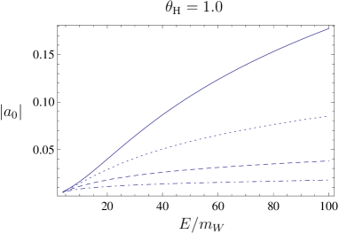
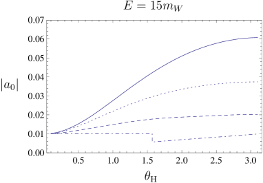
Refer to caption
Refer to caption
Figure 4: The s-wave amplitude as functions of $E$ and $\theta_{\rm H}$. The solid, dotted, dashed, dotdashed lines correspond to $kL=30,10,3,0$, respectively.

The right plot shows the $\theta_{\rm H}$-dependence of $a_{0}(15m_{W})$. We can see from these plots that the amplitude becomes larger for larger warp factor and larger $\sin(\theta_{\rm H}/2)$.666 Notice that the period of $\theta_{\rm H}$ is $2\pi$. (See the first equation in Eq.(2.17).) In the flat limit, it decreases and has only a small $\theta_{\rm H}$-dependence. In fact, it is independent of $\theta_{\rm H}$ for $0<\theta_{\rm H}\leq\pi/2$. The small $\theta_{\rm H}$-dependence for $\pi/2<\theta_{\rm H}<\pi$ originates from the fact that the relation $m_{Z}/m_{W}=2$ no longer holds and $m_{Z}$ becomes $\theta_{\rm H}$-dependent, which is peculiar to the $SU(3)$ model. Thus the details of the small $\theta_{\rm H}$-dependence in the flat case is model-dependent.

In the above calculation, we have chosen the value of the gauge coupling as $g_{4}^{2}=0.1$. Since the tree-level amplitude is proportional to $g_{4}^{2}$, it becomes four times larger if we take $g_{4}$ as the weak gauge coupling in the standard model. In this case, a scale $\Lambda$ determined by $a_{0}(\Lambda)=1$ is estimated as $\Lambda\sim 1500m_{W}$ for $\theta_{\rm H}=0.1$ and $\Lambda\sim 150m_{W}$ for $\theta_{\rm H}=1.5$ when $kL=30$, for example. This suggests that the perturbative unitarity will be violated at a lower scale for larger $\sin(\theta_{\rm H}/2)$. In order to estimate the unitarity bound, we have to consider other scattering processes and sum up all the possible final states including the KK states. Thus the real cut-off scale $\Lambda_{\rm cut}$ is expected as much lower scale than the above values of $\Lambda$. In particular, in the latter example where $m_{\rm KK}\simeq 18m_{W}$ and the Higgs mode hardly contributes to the unitarization, it is expected that $\Lambda_{\rm cut}$ becomes around 1 TeV as in the standard model without the Higgs field.

4 Summary and discussions

We have investigated the weak boson scattering in the gauge-Higgs unification, focusing on the dependence of the amplitude on the scattering energy $E$, the Wilson line phase $\theta_{\rm H}$ and the warp factor $e^{kL}$. In this paper we consider a process: $W^{+}_{L}+W^{-}_{L}\to Z_{L}+Z_{L}$ in the $SU(3)$ model as the simplest example.

The 5D propagators are useful to calculate the scattering amplitudes because we need not explicitly calculate the KK mass spectra nor perform the infinite summation over the KK modes propagating in the internal lines. We have numerically checked the equivalence theorem between the amplitudes for the longitudinal vector bosons and the (would-be) NG bosons. The correction term is read off as ${\cal O}(m_{W}^{2}/E^{2})$.

The amplitude behaves differently in the flat and the warped spacetimes. It is independent of $\theta_{\rm H}$ in the flat case, while a nontrivial $\theta_{\rm H}$-dependence comes out in the warped case. These behaviors come from the $\theta_{\rm H}$-dependences of the coupling constants among the gauge and the Higgs modes and of the KK mass scale $m_{\rm KK}$ in the case that the $W$ boson mass $m_{W}$ is fixed as an input parameter (see the beginning of Sec. 3.2.). For the non-forward (and non-backward) scattering, the amplitude approaches to a constant at high energies in both cases, but the asymptotic constant value is enhanced by a factor $kL$ in the warped case ($kL\stackrel{{\scriptstyle>}}{{{}_{\sim}}}{\cal O}(1)$), comparing to that in the flat case. On the other hand, the forward (backward) scattering amplitude grows as $E^{2}$. The s-wave amplitude grows logarithmically in high energy region just like in the standard model, and depends on $\theta_{\rm H}$ in the warped case. Thus, even if we consider only the process $W^{+}_{L}+W^{-}_{L}\to Z_{L}+Z_{L}$, the tree-level unitarity will be violated for quite large $E$. It is known, however, in higher dimensional theories, the unitarity violation appears at a lower energy, by summing up all the possible final states, exhibiting the non-renormalizability. Generically the amplitude is enhanced in the warped case for $\theta_{\rm H}={\cal O}(1)$. This suggests that the tree-level unitarity will be violated at a lower scale in the warped case than the flat case.

In Ref. [12], three separate scales that determine the dynamics of the scattering process are introduced, i.e., the electroweak breaking scale $v$, the Higgs boson decay constant $f_{h}$,777 This is the composite scale of the Higgs boson in the holographic dual picture. and the KK scale $m_{\rm KK}$. In our notation, these scales are related to each other as $v=f_{h}\theta_{\rm H}/2$ and $f_{h}=\sqrt{2}/(g_{5}\sqrt{L})=\sqrt{2}m_{\rm KK}/(\pi g_{4})$ in the flat case, and $v=f_{h}\sin(\theta_{\rm H}/2)$ and $f_{h}\simeq 2\sqrt{k}e^{-kL}/g_{5}\simeq 2m_{\rm KK}/(\pi g_{4}\sqrt{kL})$ in the warped case. In the terminology of Ref. [12], the case of $\theta_{\rm H}\ll 1$ is referred to as the β€˜Higgs limit’, and the case of $\theta_{\rm H}={\cal O}(1)$ is as the β€˜Higgsless limit’. The Higgs boson unitarizes the scattering process in the former while it does not (or does only partly) in the latter.

For the purpose of estimating the scale of the unitarity violation, we should extend our analysis for the following points. We should take into account the Higgs mass, which is induced by the quantum effect, and the decay widths of the weak bosons. The latter is necessary to discuss the process: $W^{+}_{L}+W^{-}_{L}\to W^{+}_{L}+W^{-}_{L}$, for example. The infrared singularity for the forward scattering of this process is smeared out by taking into account the width of the $W$ boson. Furthermore, we have to sum up all the possible final states including the KK states to discuss the unitarity. Since the $SU(3)$ model is a toy model, we should work in a more realistic model, for example, the $SO(5)\times U(1)$ model [9, 10, 11]. In the flat spacetime, the spectrum of the latter model has a qualitatively different $\theta_{\rm H}$-dependence from the former due to the nontrivial boundary conditions of the 5D gauge fields.888 These boundary conditions are effectively obtained from the orbifold ones by introducing some boundary terms. Each mass eigenvalue is not a linear function of $\theta_{\rm H}$ (see Fig. 1 in Ref. [11]) in contrast to the $SU(3)$ model. This difference may affects the $\theta_{\rm H}$-independence of the scattering amplitude found in the our model. These issues will be discussed in a subsequent paper.


Acknowledgments

The authors would like to thank Y. Hosotani, M. Tanabashi and K. Tobe for useful discussions and comments. This work was supported in part by the Japan Society for the Promotion of Science (T.Y.) and by Special Postdoctoral Researchers Program at RIKEN (Y.S.).

Appendix A Bases of mode functions

Here we define bases of mode functions, following Ref. [21]. The functions $C_{0}(y,m)$ and $S_{0}(y,m)$ are defined as two independent solutions to

$$\left(\frac{d}{dy}e^{-2\sigma}\frac{d}{dy}+m^{2}\right)f=0,$$ (A.1)

with initial conditions

$\displaystyle C_{0}(0,m)\!\!\!$ $\displaystyle=\!\!\!$ $\displaystyle 1,\;\;\;C^{\prime}_{0}(0,m)=0,$
$\displaystyle S_{0}(0,m)\!\!\!$ $\displaystyle=\!\!\!$ $\displaystyle 0,\;\;\;S^{\prime}_{0}(0,m)=me^{-\sigma(L)}.$ (A.2)

For the derivation of 5D propagators in Appendix B, it is convenient to define another basis functions $C_{L}(y,m)$ and $S_{L}(y,m)$ with initial conditions

$\displaystyle C_{L}(L,m)\!\!\!$ $\displaystyle=\!\!\!$ $\displaystyle 1,\;\;\;C^{\prime}_{L}(L,m)=0,$
$\displaystyle S_{L}(L,m)\!\!\!$ $\displaystyle=\!\!\!$ $\displaystyle 0,\;\;\;S^{\prime}_{L}(L,m)=me^{\sigma(L)}.$ (A.3)

From the Wronskian relation, the above functions satisfy

$\displaystyle C_{0}(y,m)S^{\prime}_{0}(y,m)-S_{0}(y,m)C^{\prime}_{0}(y,m)$ (A.4)
$\displaystyle=\!\!\!$ $\displaystyle C_{L}(y,m)S^{\prime}_{L}(y,m)-S_{L}(y,m)C^{\prime}_{L}(y,m)=me^{2\sigma(y)-\sigma(L)}.$

The two bases are related to each other by

$\displaystyle C_{L}(y,m)\!\!\!$ $\displaystyle=\!\!\!$ $\displaystyle\frac{e^{-\sigma(L)}}{m}\left\{S^{\prime}_{0}(L,m)C_{0}(y,m)-C^{\prime}_{0}(L,m)S_{0}(y,m)\right\},$
$\displaystyle S_{L}(y,m)\!\!\!$ $\displaystyle=\!\!\!$ $\displaystyle-\left\{S_{0}(L,m)C_{0}(y,m)-C_{0}(L,m)S_{0}(y,m)\right\}.$ (A.5)
Flat spacetime


In the flat spacetime, i.e., $\sigma(y)=0$, the basis functions are reduced to

$\displaystyle C_{0}(y,m)\!\!\!$ $\displaystyle=\!\!\!$ $\displaystyle\cos(my),\;\;\;S_{0}(y,m)=\sin(my),$
$\displaystyle C_{L}(y,m)\!\!\!$ $\displaystyle=\!\!\!$ $\displaystyle\cos\left\{m(y-L)\right\},\;\;\;S_{L}(y,m)=\sin\left\{m(y-L)\right\}.$ (A.6)
Randall-Sundrum spacetime


In the Randall-Sundrum spacetime, i.e., $\sigma(y)=ky$, the basis functions are written in terms of the Bessel functions as

$\displaystyle C_{0}(y,m)\!\!\!$ $\displaystyle=\!\!\!$ $\displaystyle\frac{\pi m}{2k}e^{ky}\left\{Y_{0}\left(\frac{m}{k}\right)J_{1}\left(\frac{m}{k}e^{ky}\right)-J_{0}\left(\frac{m}{k}\right)Y_{1}\left(\frac{m}{k}e^{ky}\right)\right\},$
$\displaystyle S_{0}(y,m)\!\!\!$ $\displaystyle=\!\!\!$ $\displaystyle-\frac{\pi m}{2k}e^{k(y-L)}\left\{Y_{1}\left(\frac{m}{k}\right)J_{1}\left(\frac{m}{k}e^{ky}\right)-J_{1}\left(\frac{m}{k}\right)Y_{1}\left(\frac{m}{k}e^{ky}\right)\right\},$
$\displaystyle C_{L}(y,m)\!\!\!$ $\displaystyle=\!\!\!$ $\displaystyle\frac{\pi m}{2k}e^{ky}\left\{Y_{0}\left(\frac{m}{k}e^{kL}\right)J_{1}\left(\frac{m}{k}e^{ky}\right)-J_{0}\left(\frac{m}{k}e^{kL}\right)Y_{1}\left(\frac{m}{k}e^{ky}\right)\right\},$
$\displaystyle S_{L}(y,m)\!\!\!$ $\displaystyle=\!\!\!$ $\displaystyle-\frac{\pi m}{2k}e^{ky}\left\{Y_{1}\left(\frac{m}{k}e^{kL}\right)J_{1}\left(\frac{m}{k}e^{ky}\right)-J_{1}\left(\frac{m}{k}e^{kL}\right)Y_{1}\left(\frac{m}{k}e^{ky}\right)\right\}.$

Appendix B Derivation of 5D propagators

Here we derive explicit forms of 5D propagators. We take the same strategy as in the appendix of Ref. [14]. Since the 4D vector part $A_{\mu}$ and the gauge-scalar part $A_{y}$ are decoupled at the quadratic level with our choice of the gauge-fixing function, the mixed components of the propagator $\langle 0|TA_{\mu}^{\alpha}(p,y)A_{y}^{\beta}(-p,y^{\prime})|0\rangle$ vanish. In this section, we work in the Scherk-Schwarz basis defined by (2.9) and (2.10).

B.1 Vector propagator

The gauge index $\alpha=1,\cdots,8$ is decomposed into two parts as $a=1,2,3^{\prime},8^{\prime}$ and $\hat{a}=4,5,6,7$, according to the $Z_{2}$-parities of $A_{\mu}^{\alpha}$. Then the 5D propagator $iG_{\mu\nu}^{\alpha\beta}(p,y,y^{\prime})\equiv\langle 0|TA_{\mu}^{\alpha}(p,y)A_{\nu}^{\beta}(-p,y^{\prime})|0\rangle$ satisfies

$$\left[\left\{\partial_{y}^{2}-2\sigma^{\prime}\partial_{y}-e^{2\sigma}p^{2}\right\}\delta_{\mu}^{\;\;\nu}+e^{2\sigma}\left(\frac{1}{\xi}-1\right)p_{\mu}p^{\nu}\right]G^{\alpha\beta}_{\nu\rho}(p,y,y^{\prime})=e^{2\sigma}\eta_{\mu\rho}\delta^{\alpha\beta}\delta(y-y^{\prime}),$$ (B.1)

with the boundary conditions,

$\displaystyle\partial_{y}G_{\mu\nu}^{a\beta}(p,0,y^{\prime})=G_{\mu\nu}^{\hat{a}\beta}(p,0,y^{\prime})=0,$
$\displaystyle\left(R_{\theta}\right)^{a\gamma}\partial_{y}G_{\mu\nu}^{\gamma\beta}(p,L,y^{\prime})=\left(R_{\theta}\right)^{\hat{a}\gamma}G_{\mu\nu}^{\gamma\beta}(p,L,y^{\prime})=0,$ (B.2)

where a constant matrix $R_{\theta}$ is a rotation matrix for the indices of the adjoint representation corresponding to a transformation by $\Omega(L)$ defined in (2.10), i.e.,

$$\left(R_{\theta}\right)^{\alpha\beta}A_{M}^{\beta}=\left[\Omega^{-1}(L)A_{M}\Omega(L)\right]^{\alpha}\equiv{\rm tr}\left\{\lambda^{\alpha}\Omega^{-1}(L)A_{M}\Omega(L)\right\}.$$ (B.3)

We can decompose $G_{\mu\nu}^{\alpha\beta}(p,y,y^{\prime})$ into the following two parts.

$$G_{\mu\nu}^{\alpha\beta}(p,y,y^{\prime})=\left(\eta_{\mu\nu}-\frac{p_{\mu}p_{\nu}}{p^{2}}\right)G_{\rm T}^{\alpha\beta}(y,y^{\prime},\left|p\right|)+\frac{p_{\mu}p_{\nu}}{p^{2}}G_{\rm S}^{\alpha\beta}(y,y^{\prime},\left|p\right|),$$ (B.4)

where $\left|p\right|\equiv\sqrt{-p^{2}}$. The first and the second terms correspond to the propagators for $A_{\mu}^{(n)}$ and $A_{\rm S}^{(n)}$, respectively. Writing $G_{\rm T}^{\alpha\beta}(y,y^{\prime},\left|p\right|)$ as

$$G_{\rm T}^{\alpha\beta}(y,y^{\prime},\left|p\right|)=\vartheta(y-y^{\prime})G_{\rm T>}^{\alpha\beta}(y,y^{\prime},\left|p\right|)+\vartheta(y^{\prime}-y)G_{\rm T<}^{\alpha\beta}(y,y^{\prime},\left|p\right|),$$ (B.5)

the solutions to (B.1) satisfying (B.2) are given in the matrix notation for the index $\alpha=(a,\hat{a})$ by

$\displaystyle G_{\rm T<}(y,y^{\prime},\left|p\right|)\!\!\!$ $\displaystyle=\!\!\!$ $\displaystyle{\cal M}_{0}(y,\left|p\right|)\alpha_{\rm T<}(y^{\prime},\left|p\right|),$
$\displaystyle R_{\theta}G_{\rm T>}(y,y^{\prime},\left|p\right|)\!\!\!$ $\displaystyle=\!\!\!$ $\displaystyle{\cal M}_{L}(y,\left|p\right|)\alpha_{\rm T>}(y^{\prime},\left|p\right|),$ (B.6)

where

$${\cal M}_{0}\equiv\begin{pmatrix}C_{0}\cdot\mbox{\boldmath$1$}_{4}&\\ &S_{0}\cdot\mbox{\boldmath$1$}_{4}\end{pmatrix},\;\;\;{\cal M}_{L}\equiv\begin{pmatrix}C_{L}\cdot\mbox{\boldmath$1$}_{4}&\\ &S_{L}\cdot\mbox{\boldmath$1$}_{4}\end{pmatrix}.$$ (B.7)

The unknown matrix functions $\alpha_{\rm T<}(y^{\prime},\left|p\right|)$ and $\alpha_{\rm T>}(y^{\prime},\left|p\right|)$ are determined by imposing the following matching conditions at $y=y^{\prime}$. The continuity of $G_{\rm T}$ at $y=y^{\prime}$ leads to the condition

$$G_{\rm T<}(y,y,\left|p\right|)=G_{\rm T>}(y,y,\left|p\right|),$$ (B.8)

and we obtain from (B.1) the condition

$$\left\{\partial_{y}G_{\rm T>}(y,y^{\prime},\left|p\right|)-\partial_{y}G_{\rm T<}(y,y^{\prime},\left|p\right|)\right\}_{y^{\prime}\to y}=e^{2\sigma(y)}.$$ (B.9)

Using these conditions, we obtain the 5D propagators as

$\displaystyle G_{\rm T<}(y,y^{\prime},\left|p\right|)\!\!\!$ $\displaystyle=\!\!\!$ $\displaystyle e^{2\sigma(L)}{\cal M}_{0}(y,\left|p\right|){\cal W}^{-1}(\left|p\right|){\cal M}_{L}(y^{\prime},\left|p\right|)R_{\theta},$
$\displaystyle G_{\rm T>}(y,y^{\prime},\left|p\right|)\!\!\!$ $\displaystyle=\!\!\!$ $\displaystyle\left\{G_{\rm T<}(y^{\prime},y,\left|p\right|)\right\}^{t},$ (B.10)

where

$\displaystyle{\cal W}(\left|p\right|)\!\!\!$ $\displaystyle\equiv\!\!\!$ $\displaystyle e^{-2\sigma(y)+2\sigma(L)}\left({\cal M}^{\prime}_{L}R_{\theta}{\cal M}_{0}-{\cal M}_{L}R_{\theta}{\cal M}^{\prime}_{0}\right)(y,\left|p\right|)$ (B.11)

is $y$-independent from the Wronskian relation (A.4).

The part of the scalar modes $G_{\rm S}(y,y^{\prime},\left|p\right|)$ is obtained in a similar way, and it is related to $G_{\rm T}(y,y^{\prime},\left|p\right|)$ as

$$G_{\rm S}(y,y^{\prime},\left|p\right|)=G_{\rm T}(y,y^{\prime},\left|p\right|/\sqrt{\xi}).$$ (B.12)

B.2 Gauge-scalar propagator

Next we consider the propagators for the gauge-scalar modes. The 5D propagator $iG_{yy}^{\alpha\beta}(y,y^{\prime},\left|p\right|)\equiv\langle 0|TA_{y}^{\alpha}(p,y)A_{y}^{\beta}(-p,y^{\prime})|0\rangle$ satisfies

$$\left\{\xi\partial_{y}^{2}e^{-2\sigma}-p^{2}\right\}G_{yy}^{\alpha\beta}(y,y^{\prime},\left|p\right|)=e^{2\sigma}\delta^{\alpha\beta}\delta(y-y^{\prime}),$$ (B.13)

with the boundary conditions,

$\displaystyle G_{yy}^{a\beta}(0,y^{\prime},\left|p\right|)\!\!\!$ $\displaystyle=\!\!\!$ $\displaystyle\partial_{y}\left\{e^{-2\sigma}G_{yy}^{\hat{a}\beta}\right\}(0,y^{\prime},\left|p\right|)=0,$ (B.14)
$\displaystyle\left(R_{\theta}\right)^{a\gamma}G_{yy}^{\gamma\beta}(L,y^{\prime},\left|p\right|)\!\!\!$ $\displaystyle=\!\!\!$ $\displaystyle\partial_{y}\left\{e^{-2\sigma}\left(R_{\theta}\right)^{\hat{a}\gamma}G_{yy}^{\gamma\beta}\right\}(L,y^{\prime},\left|p\right|)=0.$ (B.15)

These can be solved by the same manner as in the previous subsection. We find that $G_{yy}(y,y^{\prime},\left|p\right|)$ is related to $G_{\rm S}(y,y^{\prime},\left|p\right|)$ as

$\displaystyle G_{yy<}(y,y^{\prime},\left|p\right|)\!\!\!$ $\displaystyle=\!\!\!$ $\displaystyle-\frac{1}{p^{2}}\partial_{y}\partial_{y^{\prime}}G_{\rm S<}(y,y^{\prime},\left|p\right|),$
$\displaystyle G_{yy>}(y,y^{\prime},\left|p\right|)\!\!\!$ $\displaystyle=\!\!\!$ $\displaystyle-\frac{1}{p^{2}}\partial_{y}\partial_{y^{\prime}}G_{\rm S>}(y,y^{\prime},\left|p\right|).$ (B.16)

References

  • [1] C. Csaki, C. Grojean, H. Murayama, L. Pilo, and J. Terning, Phys. Rev. D69 (2004) 055006.
  • [2] D.B. Fairlie, Phys. Lett. B82 (1979) 97; J. Phys. G5 (1979) L55; N. Manton, Nucl. Phys. B158 (1979) 141; P. Forgacs and N. Manton, Commun. Math. Phys. 72 (1980) 15.
  • [3] Y. Hosotani, Phys. Lett. B126 (1983) 309; 129 (1983) 193; Phys. Rev. D29 (1984) 731.
  • [4] H. Hatanaka, T. Inami and C.S. Lim, Mod. Phys. Lett. A13 (1998) 2601; A. Pomarol and M. Quiros, Phys. Lett. B438 (1998) 255.
  • [5] N. Haba, Y. Hosotani, Y. Kawamura and T. Yamashita, Phys. Rev. D70 (2004) 015010; N. Haba and T. Yamashita, JHEP 0402 (2004) 059; ibid. 0404 (2004) 016; N. Haba, S. Matsumoto, N. Okada and T. Yamashita, JHEP 0602 (2006) 073; Prog. Theor. Phys. 120 (2008) 77; N. Haba, K. Takenaga and T. Yamashita, Phys. Lett. B615 (2005) 247; N. Maru and T. Yamashita, Nucl. Phys. B754 (2006) 127; Y. Hosotani, N. Maru, K. Takenaga and T. Yamashita, Prog. Theor. Phys. 118 (2007) 1053; C. Csaki, C. Grojean and H. Murayama, Phys. Rev. D67 (2003) 085012; G. Burdman and Y. Nomura, Nucl. Phys. B656 (2003) 3; C. A. Scrucca, M. Serone and L. Silvestrini, Nucl. Phys. B669 (2003) 128.
  • [6] L.J. Hall, Y. Nomura and D. Tucker-Smith, Nucl. Phys. B639 (2002) 307; N. Haba and Y. Shimizu, Phys. Rev. D67 (2003) 095001 [Erratum-ibid.  D69 (2004) 059902]; K.w. Choi, N.y. Haba, K. S. Jeong, K.i. Okumura, Y. Shimizu and M. Yamaguchi, JHEP 0402 (2004) 037;
  • [7] R. Contino, Y. Nomura and A. Pomarol, Nucl. Phys. B671 (2003) 148; K. Oda and A. Weiler, Phys. Lett. B606 (2005) 408; Y. Hosotani and M. Mabe, Phys. Lett. B615 (2005) 257;
  • [8] Y. Hosotani, S. Noda, Y. Sakamura and S. Shimasaki, Phys. Rev. D73 (2006) 096006.
  • [9] K. Agashe, R. Contino and A. Pomarol, Nucl. Phys. B719 (2005) 165; M. Carena, E. Ponton, J. Santiago and C.E.M. Wagner, Phys. Rev. D76 (2007) 035006; Y. Hosotani, K. Oda, T. Ohnuma and Y. Sakamura, Phys. Rev. D78 (2008) 096002; Y. Hosotani and Y. Kobayashi, Phys. Lett. B674 (2009) 192.
  • [10] Y. Sakamura and Y. Hosotani, Phys. Lett. B645 (2007) 442; Y. Sakamura, Phys. Rev. D76 (2007) 065002.
  • [11] Y. Hosotani and Y. Sakamura, Prog. Theor. Phys. 118 (2007) 935.
  • [12] A. Falkowski, S. Pokorski and J.P. Roberts, JHEP 0712 (2007) 063.
  • [13] L. Randall and R. Sundrum, Phys. Rev. Lett. 83 (1999) 3370.
  • [14] T. Gherghetta and A. Pomarol, Nucl. Phys. B602 (2001) 3.
  • [15] A. Falkowski and M. PΓ©rez-Victoria, arXiv:0810.4940.
  • [16] J.M. Cornwall, D.N. Levin and G. Tiktopoulos, Phys. Rev. D10 (1974) 1145; B.W. Lee, C. Quigg and H.B. Thacker, Phys. Rev. D16 (1977) 1519; M.S. Chanowitz and M.K. Gaillard, Nucl. Phys. B261 (1985) 379.
  • [17] R. Sekhar Chivukula, D.A. Dicus and H.J. He, Phys. Lett. B525 (2002) 175; Y. Abe, N. Haba, Y. Higashide, K. Kobayashi and M. Matsunaga, Prog. Theor. Phys. 109 (2003) 831; Y. Abe, N. Haba, K. Hayakawa, Y. Matsumoto, M. Matsunaga and K. Miyachi, Prog. Theor. Phys. 113 (2005) 199.
  • [18] H.J. He, Y.P. Kuang and X. Li, Phys. Rev. D49 (1994) 4842; H.J. He and W.B. Kilgore, Phys. Rev. D55 (1997) 1515.
  • [19] R. Sekhar Chivukula, H.J. He, M. Kurachi, E.H. Simmons and M. Tanabashi, Phys. Rev. D78 (2008) 095003.
  • [20] L. Durand, J.M. Johnson and J.L. Lopez, Phys. Rev. Lett. 64 (1990) 1215; Phys. Rev. D45 (1992) 3112; G. Passarino, Nucl. Phys. B343 (1990) 31; L. Durand, J.M. Johnson and P.N. Maher, Phys. Rev. D44 (1991) 127.
  • [21] A. Falkowski, Phys. Rev. D75 (2007) 025017.