CaSPA - an Algorithm for Calculation of the Size of Percolating Aggregates

Abstract

We present an algorithm (CaSPA) which accounts for the effects of periodic boundary conditions in the calculation of size of percolating aggregated clusters. The algorithm calculates the gyration tensor, allowing for a mixture of infinite (macroscale) and finite (microscale) principle moments. Equilibration of a triblock copolymer system from a disordered initial configuration to a hexagonal phase is examined using the algorithm.

Keywords: Aggregation, Periodic Boundary Conditions, Triblock Copolymer
PACS: 02.70.Ns, 61.46.Be, 64.70.mf, 82.35.Jk

1 Introduction

Structures obtained from surfactant solutions or block copolymers and their properties are of interest in many fields [1]. The processes that occur during these transitions can be relevant in polymer processing for the fabrication of nanostructured materials [2], especially in cases where the reversibility between structures is of interest. In biophysics, the lamellar to reverse hexagonal phase transition is considered as the first step in understanding membrane fusion [3, 4, 5].

Order-disorder and order-order transitions have been studied experimentally, theoretically and using computer simulations. Much of the theoretical and simulation work has focused on the identification of different ordered structures that can be obtained when changing the architecture of the amphiphilic molecule and the system conditions [6]. Nevertheless, the dynamic processes that describe the order-disorder or order-order transitions are also important. Processes such as micelle formation and stabilization, sphere to rod transitions, bilayer breakdown and structural changes during the formation of nanostructured materials have attracted much attention [7, 8].

Groot and Madden used dissipative particle dynamics (DPD) simulations to describe the formation of an hexagonal phase from a disordered phase, where an unstable gyroid phase appears as an intermediate using DPD simulations [9]. More recently, Soto-Figueroa et al. described the dynamics of different order-order transitions in polystyrene-polyisoprene diblock copolymers [10]. The transition between hexagonally packed cylinders to an array of body centred cube spheres is a result of undulations in the cylinders that eventually break into ellipsoids to latter form spheres. They also describe the transition from a bicontinuous structure to a lamellar phase going through an intermediate phase containing infinite cylinders, not observed by Groot and Madden, before a lamellar phase is obtained. Dynamics of the formation of ordered phases has also been reported for a variety of surfactant architectures [11], but most of the results are limited to a collection of snapshots at different times during the simulation. In some cases, an order parameter is defined and used to determine the evolution of the observed phases, which requires the calculation of the structure factor [12].

For any simulation approach which seeks to model mesoscale aggregates from the microscale, the aggregates will appear infinite, that is, they will percolate, spanning the periodic boundary conditions (PBCs) of the simulation. The dimensionality of the aggregate (whether one dimensional for cylinders, two dimensional for lamellae, or three dimensional for network structures) will set the dimensionality of this percolation. Algorithms exist to identify aggregates within a simulation configuration (principally, the Hoshen-Kopelman (H-K) algorithm [13]), however, once identified, the aggregate must be properly characterised.

The standard approach to characterisation of the size and shape of an aggregate is diagonalization of its gyration tensor $\mathbf{S}$. If the positions of the $N$ particles in the aggregate relative to its center of mass are given by $\left\{\mathbf{r}_{i}\right\}$, the gyration tensor is given by:

$$S_{\alpha\beta}=\frac{1}{N}\sum_{i=1}^{N}r_{i}^{\alpha}r_{i}^{\beta}$$ (1)

where $r_{i}^{\alpha}$ denotes the $\alpha$’th component of the vector $\mathbf{r}$, and $S_{\alpha\beta}$ indicates the $\left(\alpha,\beta\right)$’th element of the tensor $\mathbf{S}$. The eigenvectors of this tensor (the “principal axes”) give the orientation of the aggregate, and the associated eigenvalues (the “principle moments”) give the length scales of the aggregate along these vectors.

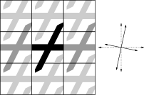
A naive implementation of Eqn. 1 for a percolating aggregate, using only the coordinates from the microscale aggregate identified within the simulation boundary conditions, will produce incorrect results. First, such an implementation will not identify the correct principle moments; since the full, macroscale aggregate is percolating, at least one principle moment is infinite by definition. Second, there is some subtlety as to which periodic images of a particle to include in the calculation, such that only particles within a single aggregate should be included, and particles within images of the aggregate must be excluded. Finally, by not explicitly dealing with the percolation of the aggregate, pathological configurations may result in an incorrectly oriented gyration tensor. If the principle axes are incorrectly oriented, then equivalently the principle moments will be wrong. This is illustrated in 1.

Figure 1: An aggregate (filled area) repeated across periodic boundary conditions. The micro-scale aggregate identified from the structure is shown by the black filled area, and the gyration tensor for this aggregate is schematically illustrated by the full arrows. To calculate the gyration tensor for the true percolating aggregate, only particles in the black and dark shaded areas should be included. The gyration tensor for the percolating aggregate is schematically illustrated by the dotted arrows. The two gyration tensors are not aligned. Note that the percolating aggregate is infinite in the horizontal direction, whereas the longest principle component of the microscale aggregate lies closest to the vertical direction.

In this work, we present an algorithm (Calculation of Size of Percolating Aggregates, or CaSPA) to deal with these issues. The algorithm is demonstrated through application to aggregates formed in a triblock copolymer system, simulated using dissipative particle dynamics (DPD) [14, 15, 16, 17].

2 Methods

2.1 CaSPA algorithm

Consider an aggregate composed of $N$ particles $\left\{\mathbf{r}_{i}\right\}$, with gyration tensor $\mathbf{S}$. The aggregate exists within PBCs, and is a percolating cluster, that is, particles within the aggregate are connected to particles in certain periodic images of the aggregate. We denote the set of translation vectors between the contacting images $\left\{\mathbf{p}^{\prime}_{i}\right\}$; these can be reduced to a combination of $n_{p}$ linearly independent vectors $\left\{\mathbf{p}_{i}\right\}$. The aggregate is therefore percolating in $n_{p}$ dimensions. We seek the gyration tensor $\mathbf{S}^{macro}$ for the full macroscale aggregate, made up of the combination of individual, contacting aggregates across the periodic boundaries. If we include $n_{i}$ image aggregates along each of the $\mathbf{p}$ vectors, this gyration tensor will be given by:

$$S_{\alpha\beta}^{macro} = \frac{1}{Nn_{i}^{n_{p}}}\left(\sum_{k_{1}=-(n_{i}-1)/2}^{(n_{i}-1)/2}\dots\sum_{k_{n_{p}}=-(n_{i}-1)/2}^{(n_{i}-1)/2}\right)\times$$ (2)

$$\sum_{i=1}^{N}\left(r_{i}^{\alpha}+\sum_{j=1}^{n_{p}}k_{j}p_{j}^{\alpha}\right)\left(r_{i}^{\beta}+\sum_{j^{\prime}=1}^{n_{p}}k_{j^{\prime}}p_{j^{\prime}}^{\beta}\right)$$

Multiplying out, through the symmetry of the sum limits, and considering that since the origin is at the center of mass $\sum_{i}p_{i}^{\alpha}=0$, we find:

$$S_{\alpha\beta}^{macro}=S_{\alpha\beta}+\frac{1}{12}\left(n_{i}-1\right)\left(n_{i}+1\right)Q_{\alpha\beta}$$ (3)

where the tensor $\mathbf{Q}$ is given by:

$$Q_{\alpha\beta}=\sum_{i=1}^{n_{p}}p_{i}^{\alpha}p_{i}^{\beta}$$ (4)

Note the similarity between the form of $\mathbf{Q}$ and the definition of the gyration tensor (Eq. 1). The tensor $\mathbf{Q}$ can be considered as the normalized gyration tensor for a coarse-grained representation of the macroscale aggregate, with one point mass per image. We seek to diagonalise $\mathbf{S}^{macro}$, giving three eigenvectors (the principle axes) $\mathbf{A}_{i}$, and three corresponding eigenvalues (the principle components) $\lambda_{i}^{2}$, $\lambda_{1}^{2}\leq\lambda_{2}^{2}\leq\lambda_{3}^{2}$.

As $n_{i}$ tends to infinity (the bulk limit), the gyration tensor $\mathbf{S}^{macro}$ becomes dominated by the matrix $\mathbf{Q}$. This determines the orientation of the macroscale aggregate in space. However, provided the aggregate does not percolate in all dimensions, one or more of the eigenvalues of $\mathbf{Q}$ will be zero, hence $\mathbf{Q}$ is singular. By performing singular value decomposition [18] on $\mathbf{Q}$, we can identify the range $\mathbf{U}$ of $\mathbf{Q}$, the set of $n_{p}$ eigenvectors with non-zero eigenvalues, and the nullspace $\mathbf{V}$ of $\mathbf{Q}$, a set of orthogonal eigenvectors for which the eigenvalues are zero. The macroscale aggregate will have infinite principle components in the range (where $\mathbf{Q}$ will dominate), and finite principle components in the nullspace (where only $\mathbf{S}$ contributes).

For tensors $\mathbf{Q}$ with a single vector $\mathbf{V}_{1}$ in the nullspace, the orientation of the finite principle component of the macroscale aggregate is given by $\mathbf{A}_{1}=\mathbf{V}_{1}$ and the value of the finite principal component is given by the projection of $\mathbf{S}$ along this vector, $\lambda_{1}^{2}=\mathbf{V}_{1}^{T}\mathbf{S}\mathbf{V}_{1}$. The remaining two principle components are infinite, $\lambda_{2}^{2}=\lambda_{3}^{2}=\infty$, with the corresponding principle axes lying along the range, $\mathbf{A}_{2}=\mathbf{U}_{2}$ and $\mathbf{A}_{3}=\mathbf{U}_{3}$.

For a tensor $\mathbf{Q}$ with two vectors ($\mathbf{V}_{1}$ and $\mathbf{V}_{2}$) in the nullspace, the orientation of the infinite principle component $\lambda_{3}^{2}=\infty$ of the macroscale aggregate is given by $\mathbf{A}_{3}=\mathbf{U}_{3}$. The vectors describing the finite principal components will be linear combinations of $\mathbf{V}_{1}$ and $\mathbf{V}_{2}$, which will be a pair of vectors which are orthogonal to the range $\mathbf{U}_{3}$, but are otherwise arbitrary. To find the finite principle axes, we must project the matrix $\mathbf{S}$ into the plane given by $\mathbf{V}$. This results in a two dimensional gyration tensor given by $\left[\begin{array}[]{c}\mathbf{V}_{1}^{T}\\ \mathbf{V}_{2}^{T}\end{array}\right]\mathbf{S}\left[\begin{array}[]{cc}\mathbf{V}_{1}&\mathbf{V}_{2}\end{array}\right]$, with two-dimensional eigenvectors $\mathbf{A}^{\prime}_{1}$ and $\mathbf{A}^{\prime}_{2}$, and corresponding eigenvalues giving the principle components, $\lambda_{1}^{2}$ and $\lambda_{2}^{2}$. The orientations of the principle components are given by $\mathbf{A}_{i}=\mathbf{A}^{\prime}_{i}\left[\mathbf{V}_{1}\,\mathbf{V}_{2}\right]$, that is, the eigenvectors $\mathbf{A}^{\prime}_{i}$ give the appropriate linear combinations of the nullspace vectors to give the principle axes.

The two remaining cases are tensors $\mathbf{Q}$ with no nullspace, representing a percolating macroscale aggregate which is infinite in all directions ($\lambda_{1}^{2}=\lambda_{2}^{2}=\lambda_{3}^{2}=\infty$), and tensors $\mathbf{Q}$ with a three-dimensional nullspace, representing aggregates with no self contacts, which can be treated entirely from the aggregate gyration tensor $\mathbf{S}$.

From this, the algorithm to calculate the principle components and axes of the macroscale aggregate must perform the following steps:

1. Identify the aggregate coordinates $\left\{\mathbf{r}_{i}\right\}$, and calculate the aggregate gyration tensor $\mathbf{S}$.

2. Identify the set of self-contact vectors, $\left\{\mathbf{p}^{\prime}_{i}\right\}$, and reduce it to a linearly dependent set, $\left\{\mathbf{p}_{i}\right\}$.

3. Calculate the tensor $\mathbf{Q}\left(\left\{\mathbf{p}_{i}\right\}\right)$, and find its range $\mathbf{U}$ and nullspace $\mathbf{V}$.

4. Calculate the projection of the gyration tensor $\mathbf{S}$ onto the nullspace $\mathbf{V}$.

5. Return the macroscale aggregate principle axes (the range $\mathbf{U}$ and unit vector projections of the nullspace $\mathbf{V}$ onto the gyration tensor $\mathbf{S}$) and principle components (infinity for axes corresponding to the range, and the length of the vector projections of the nullspace $\mathbf{V}$ onto the gyration tensor $\mathbf{S}$ for the remaining components).

We now describe how such an algorithm may be implemented.

2.1.1 Identification of the aggregate coordinates

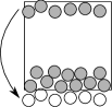
The H-K algorithm is suitable for initial identification of an aggregate from a particle configuration. However, to deal with an aggregate which crosses PBC’s, an extra step is necessary. In simulation coordinates, aggregates will often consist of a number of disjunct segments, connected across the PBC’s (see 2). The first task of the algorithm, once the initial $N$-particle aggregate has been identified, is to “stitch” these disjunct segments into a single, fully connected object. The minimum image convention cannot be used for this, since the positions of particles in images of the aggregate may become mixed with positions of particles in the aggregate during calculation of the gyration tensor, giving incorrect results.

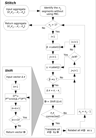
To “stitch” an aggregate together, the coordinates $\left\{\mathbf{r}_{i}\right\}$ of the particles in the aggregate are passed to a version of the cluster identification algorithm which does not recognise the PBCs. This identifies the $n_{d}$ disjoint segments, and returns a list $\left\{l_{i}\right\}$, labelling each of the $N$ particles in $\left\{\mathbf{r}_{i}\right\}$ according to which subcluster that particle is a member of. The algorithm then loops over all pairs of particles, until it finds a pair $\left(i,j\right)$ such that $l_{i}\neq l_{j}$, and which contact across PBCs. Having found such a pair, all particles with label $l_{i}$ are relabelled with $l_{j}$ and translated such that particles $i$ and $j$ are bonded without PBCs (merging disjunct clusters $l_{i}$ and $l_{j}$ into a single, connected cluster), and $n_{d}$ is decremented. This is then repeated until $n_{d}=1$, that is, there exists only a single connected cluster. Note that the resulting set of coordinates will now extend outside of the original PBCs

Figure 2: Illustration of the “stitching” process. Shaded circles represent particles within the PBC’s which form two disjunct segments of a single aggregate. Once self-contact vectors have been identified, one of these segments is translated outside of the PBC’s (open circles) such that the aggregate forms a single, connected cluster.

(see 2). A flowchart for the “stitching” algorithm is shown in Fig. 3

Figure 3: The “stitching” algorithm. Inset: the “shift” algorithm, which finds the vector between periodic images. The function rint rounds its argument to the nearest integer. The vector $\mathbf{P}$ contains the lengths of the periodic boundary conditions.

. Given this single connected cluster (the microscale aggregate), the gyration tensor $\mathbf{S}$ can be calculated as Eqn. 1.

2.1.2 Identification of the Self-Contact Vectors

Once the aggregate coordinates have been identified, the self-contact vectors can be found. The set $\left\{\mathbf{p}^{\prime}_{i}\right\}$ is easy to identify - loop across every pair of particles in the aggregate, check if they are contacting across the PBCs, and if they are, store the vector connecting the periodic images (given, in the terminology of 3, by Shift$\left(\Delta r\right)$). This set may, however, be very large, and will in general contain a large quantity of redundant data. We seek instead the linearly independent set $\left\{\mathbf{p}_{i}\right\}$, which in three dimensions may consist of a maximum of three vectors.

To find these vectors, the algorithm must loop across every pair of particles in the aggregate, checking for contact across PBCs, until a vector connecting periodic images is found. This is stored in $\mathbf{p}_{1}$. The loop then continues, until a second candidate vector $\mathbf{p}^{\prime}$ is found. The algorithm must check that this new vector is linearly independent of $\mathbf{p}_{1}$; the condition for this is that $\left|\mathbf{p}_{1}\times\mathbf{p}^{\prime}\right|\neq 0$. If $\mathbf{p}^{\prime}$ is linearly independent of $\mathbf{p}_{1}$, then the algorithm sets $\mathbf{p}_{2}=\mathbf{p}^{\prime}$. Otherwise, the algorithm continues to check candidate vectors $\mathbf{p}^{\prime}$ for linear dependence against $\mathbf{p}_{1}$.

If two linearly dependent vectors have been found, then the loop once again continues, but now candidate vectors must be checked for linear independence against $\mathbf{p}_{1}$ and $\mathbf{p}_{2}$. The condition for linear independence is now that $\det\left(\left[\mathbf{p}_{1}\,\mathbf{p}_{2}\,\mathbf{p}^{\prime}\right]\right)\neq 0$. If $\mathbf{p}^{\prime}$ is linearly independent of $\mathbf{p}_{1}$, the algorithm sets $\mathbf{p}_{3}=\mathbf{p}^{\prime}$, and terminates; the aggregate is percolating in three dimensions, hence all principle components are infinite.

Once all pairs have been checked, the algorithm is left with $n_{p}$ linearly independent self-contact vectors $\left\{\mathbf{p}_{i}\right\}$. A flowchart for the self-contact identification algorithm is shown in 4.

Figure 4: The ContactVectors algorithm.

From the vectors $\left\{\mathbf{p}_{i}\right\}$, the tensor $\mathbf{Q}$ may be calculated as Eqn. 4. This tensor is then diagonalised. There should be $n_{p}$ non-zero eigenvalues, corresponding to the eigenvectors $\left\{\mathbf{U}_{i}\right\}$ in the range of $\mathbf{Q}$, and $\left(3-n_{p}\right)$ zero eigenvalues, corresponding to the eigenvectors $\left\{\mathbf{V}_{i}\right\}$ in the nullspace of $\mathbf{Q}$.

2.1.3 Calculation of Gyration Tensor of the Infinitely Repeated Aggregate

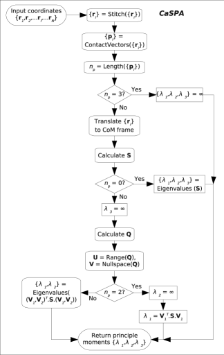
Finally, the algorithm has the aggregate gyration tensor $\mathbf{S}$, the dimensionality of percolation, $n_{p}$, and the range and nullspace of percolation, $\left\{\mathbf{U}_{i}\right\}$ and $\left\{\mathbf{V}_{i}\right\}$. The algorithm will already have terminated if the aggregate is percolating in three dimensions, returning three infinite principle components. Otherwise, the principle components and axes may be calculated by projection of $\mathbf{S}$ onto the nullspace $\mathbf{V}$, as detailed above. A full flowchart of CaSPA is shown in 5.

Figure 5: The CaSPA algorithm; “CoM frame” denotes the frame of reference where the aggregate center of mass is the origin.

2.1.4 Optimization

The algorithm as described here has been separated into parts for conceptual clarity, and as such is not optimized for speed. It is anticipated, however, that the generation of uncorrelated configurations by simulation for analysis is likely to be significantly slower than the analysis of these configurations.

The process of checking all pairs in the system means that, as presented, the time needed scales as $N^{2}$. If the definition of contact allows, the algorithm can be reduced to scaling with $N$ via construction and use of a cell list. A second obvious improvement would be to perform the identification of self-contact vectors $\left\{\mathbf{p}_{i}\right\}$ at the same time as the “stitching” algorithm, by checking for boundary-crossing contacts between particles in the same aggregate segment. While this will not change the scaling form, it should significantly reduce the constant of proportionality.

2.2 Test System

To demonstrate the algorithm, we have simulated equilibration of a triblock copolymer solution from an initial, random configuration. The simulation has been performed using dissipative particle dynamics (DPD). This is a mesoscale simulation methodology, where “particles” represent loosely-defined “fluid elements”, and move via a combination of dissipative, random and conservative interparticle forces.

Particles in the system interact via the “standard” DPD force field [16], given by:

$$U_{ij}=\begin{cases}\frac{a_{ij}}{2r_{c}}\left(r_{c}-r_{ij}\right)^{2}&r_{ij}\leq r_{c}\\ 0&r_{ij}>r_{c}\end{cases}$$ (5)

where $r_{ij}$ is the separation between particles indices $i$ and $j$, $r_{c}$ is a notional particle diameter (setting the length scale of the system), and $a_{ij}$ a parameter which depends upon the types of particles indices $i$ and $j$, setting the strength of interaction between these types. Particles which are bonded along a polymer chain also interact via a spring force, spring constant $C=4k_{B}T$ [17].

The simulated system exists within a cubic box of size $15r_{c}$, with total particle number density $\rho=3$, and is made up of $A$ and $B$ type monomers and solvent particles (type $S$). Interaction parameters for like particle types are $a_{XX}=25$, and for unlike types are $a_{SA}=a_{AB}=50$ and $a_{SB}=25$; as such, $A$-type monomers are “hydrophobic”. All $A$ and $B$ type monomers exist as part of $A_{3}B_{10}A_{3}$ triblock copolymers. The system has $4061$ solvent particles, and $379$ copolymers, giving a copolymer volume fraction of $0.6$. The simulation reduced timestep is $\Delta t=0.01$, and the simulation is run for $4\times 10^{6}$ timesteps. The initial configuration is generated by placing solvent particles and one end monomer of each copolymer randomly in the simulation box. Copolymers are grown by placing the center of the next monomer in each polymer at a random position on a sphere of radius $r_{c}$ centered on the previous monomer. The energy of this random configuration is then minimised by steepest descent to give the starting configuration for the simulation.

3 Results

Time series data of the configurational energy (decomposed into pair and spring interactions) from the simulation are shown in 6. From the point of view of energy, the random initial system configuration appears to reflect the equilibrium state well, and the system does not appear to pass through any significant energetic relaxation.

Figure 6: Configurational energy for the triblock copolymer simulation, decomposed into pair interactions ($U_{C}$) and spring force interactions ($U_{S}$), as a function of simulation time $t$. No significant energetic relaxation is observed.

“Stitched” snapshot configurations from the simulation (see 7)

Figure 7: ”Stitched” snapshot conformations from the triblock copolymer simulation. Cylinders join $A$-type monomers separated by less than $r_{c}$. Lines indicate the simulation box. a) Coexistence between large, self-contacting aggregate (lower right) and elongated micelle at $t=2\Delta t$. b) Coexistence between large, self-contacting aggregate (center), spherical micelle (top) and elongated micelle (bottom) at $t=100\Delta t$. c) Single, elongated micelle at $t=200\Delta t$. d) Large, self-contacting aggregate at $t=380\Delta t$.

indicate that the system undergoes mesophase separation, with the “hydrophobic” $A$-type monomers forming elongated aggregates, demixed from the solvent and $B$-type monomers. As such, the CaSPA algorithm has been used to study these aggregates. Pairs of $A$-type monomers are considered to be “connected” if they overlap (that is, if $r_{ij}<r_{c}$). Data for clusters smaller than 3 monomers are discarded. It should be noted that the results we present are insensitive to the definition of connectivity, being qualitatively similar across a range of definitions of connectivity from $r<0.8r_{c}$ to $r<1.2r_{c}$. This insensitivity can be explained by considering the radial distribution function between $A$-type monomers $g_{AA}(r)$

Figure 8: Radial distribution function $g_{AA}(r)$ between hydrophobic monomers.

(see 8). The nearest-neighbour peak can be seen to be at a maximum at at $r=0.825r_{c}$, and can further be seen to be distinct from the broader peak indicating aggregate structure up to $r\approx 1.2r_{c}$. As long as the cutoff for connectivity lies between these two values, the algorithm will probe nearest neighbour structure in an effective fashion.

Time series data from CaSPA for the principal gyration components of these clusters are shown in 9. Within these results, clusters of $A$-type monomers are found to be either non-percolating, or to be percolating in only one dimension. Time series data for the fraction of $A$-type monomers in clusters of each type are shown in 10. While no obvious energetic relaxation is observed, the CaSPA results suggest significant structural relaxation.

Figure 9: Principal components of the gyration tensor $\lambda_{1}\leq\lambda_{2}\leq\lambda_{3}$ for clusters of $A$-type monomers as a function of simulation time $t$. The left hand column shows principal components for non-percolating clusters. The right hand column shows principal components for clusters which are percolating in one dimension; note that, for these clusters, $\lambda_{3}=\infty$ by definition. Multiple points at a given time step denote multiple clusters of that type at a given time step.

Figure 10: Fraction of $A$-type monomers in non-percolating clusters ($f_{0}$) and in clusters which are percolating in one dimension ($f_{1}$) as a function of simulation time, $t$. Multiple points at a given time step indicate multiple clusters of that type at that time step.

The CaSPA data clearly shows that, across most of the simulation, the system is dominated by the presence of a single, large (containing more than $70\%$ of all $A$-type monomers) cluster which is percolating in one dimension. As such, we can suggest that the system is equilibrating towards a hexagonal cylindrical liquid crystal.

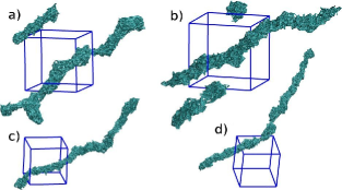
Up until $t\approx 19300\Delta t$, the percolating cluster coexists with one or more smaller, though still significant, non-percolating clusters, which appear to be micellar in character. Where only a single micelle exists, it can be seen to be extended, and approximately cylindrical ($\lambda_{1}\approx\lambda_{2}<\lambda_{3}$) (see snapshot configuration in 7(a)). The largest principle component of this micelle can be seen to be of the order of half the length of the simulation box ($\lambda_{3}\approx 7r_{c}$). Where two micelles exist, the smaller micelle is approximately spherical ($\lambda_{1}\approx\lambda_{2}\approx\lambda_{3}\approx r_{c}$), while the larger micelle is extended and approximately cylindrical (see snapshot configuration in 7(b)). The excess material contained in these micelles is absorbed into the larger cluster at $t\approx 19300\Delta t$. The smallest principal moments of gyration $\lambda_{1}$ and $\lambda_{2}$ increase at around $t\approx 19300\Delta t$, corresponding to absorption of this material into the large micelle.

After $t\approx 19300\Delta t$, the vast majority (greater than $99.5\%$) of $A$-type monomers exist in a single cluster. Across most of this time (approximately $85\%$), that cluster is percolating in one dimension (see snapshot configuration in 7(d)), however, there are five events where that cluster becomes non-percolating (see, for e.g., snapshot configuration in 7(c)). During these events, the cluster keeps approximately the same values for the smaller principal moments of gyration, while taking on a large value ($\lambda_{3}\approx 18.5r_{c}$) for the largest principal moment.

The character of the large, percolating cluster does not appear quite cylindrical from the data; the aspect ratio of the cluster is not unity, but instead $\lambda_{2}/\lambda_{1}\approx 1.9$. This value does not change significantly with time. The reason for this apparent non-cylindrical character is made clear in the “stitched” snapshot configurations (7); the cluster does not lie along a straight path, but is instead significantly curved. This suggests that the configuration is not fully equilibrated, but is suffering from a finite size effect, where the cylindrical aggregate is not aligned properly within the simulation box, and must bend in order to maintain self-contact across periodic boundaries. We suggest that the observed events where the cluster becomes non-percolating correspond to equilibration towards the correct alignment.

4 Discussion

In the previous sections, we have presented CaSPA, a novel algorithm to characterise the size and orientation of percolating aggregates, and have tested this algorithm on a triblock copolymer system. Results using CaSPA show that this system forms percolating one-dimensional aggregates. These results demonstrate the strengths of the algorithm. Configurational energy does not indicate any relaxation phenomena during the simulation (6), whereas measurement of the size of aggregated clusters clearly identifies structural relaxation (9). While the standard Hoshen-Kopelman algorithm would identify the presence of this relaxation, CaSPA allows a fuller description by identifying percolating aggregates. In the case presented here, this allows very long elongated micelles to be distinguished from true percolating cylindrical aggregates. Further, CaSPA returns the correct principle moments of gyration for branched percolating structures (such as the percolating aggregates in 7 (a) and (b)). Finally, the “stitching” step in CaSPA can be used to generate snapshot configurations of aggregates (7) which are easier to visualise than the equivalent “unstitched” configurations. Coupled with data on the size of aggregates, this clearer visualization can aid both understanding and communication of observed behaviors in simulation of mesostructured materials.

Use of CaSPA is complementary to other order parameter measurements used to describe mesophase structures. While the algorithm provides a broad range of information on the size and shape of aggregates, it does not provide information on the degree of segregation of aggregating particles from the rest of the system. As a comparative example, the $P$ order parameter proposed by Groot et al [12] provides information on the degree of segregation of particles, and can differentiate between structures, but is not intended to provide clear geometric information on those structures. In summary, CaSPA provides a useful addition to methods for identification and characterisation of mesostructured materials.

References

- [1] T. Smart et al., Nanotoday 3, 38 (2008).
- [2] H. Klok and S. Lecommandoux, Adv. Mater. 16, 1217 (2001).
- [3] D. Siegel and R. Epand, Biopys. J. 73, 3089 (1997).
- [4] S. May, D. Harries, and A. Ben-Shaul, Biophys. J. 78, 1681 (2000).
- [5] I. Koltover, T. Sladitt, J. Radler, and C. Safinya, Science 281, 78 (1998).
- [6] V. Ortiz, S. Nielsen, M. Klein, and D. Discher, J. Polym. Sci. B: Pol. Phys. 44, 1907 (2006).
- [7] M. Gradzielski, Curr. Opin. Colloid In. 9, 256 (2004).
- [8] S. Sakurai et al., Macromolecules 26, 485 (1993).
- [9] R. Groot and T. Madden, J. Chem. Phys. 108, 8713 (1998).
- [10] C. Soto-Figueroa, M. Rodriguez-Hidalgo, J. Martinez-Magadan, and L. Vicente, Macromolecules 41, 3297 (2008).
- [11] A. Khokhlov and P. Khalatur, Chem. Phys. Lett. 461, 58 (2008).
- [12] R. Groot, T. Madden, and D. Tildesley, J. Chem. Phys. 110, 9739 (1999).
- [13] J. Hoshen and R. Kopelman, Phys. Rev. B 14, 3438 (1976).
- [14] P. Hoogerbrugge and J. Koelman, Europhys. Lett. 19, 155 (1992).
- [15] J. Koelman and P. Hoogerbrugge, Europhys. Lett. 21, 363 (1993).
- [16] D. Frenkel and B. Smit, Understanding Molecular Simulation, second edition ed. (Academic Press, ADDRESS, 2002).
- [17] R. Groot and P. Warren, J. Chem. Phys. 107, 4423 (1997).
- [18] W. Press, S. Teukolsky, W. Vetterling, and B. Flannery, Numerical Recipes in C, second edition ed. (Cambridge University Press, ADDRESS, 1992).