Negative fluctuation-dissipation ratios in the backgammon model

Abstract

We analyze fluctuation-dissipation relations in the Backgammon model: a system that displays glassy behavior at zero temperature due to the existence of entropy barriers. We study local and global fluctuation relations for the different observables in the model. For the case of a global perturbation we find a unique negative fluctuation-dissipation ratio that is independent of the observable and which diverges linearly with the waiting time. This result suggests that a negative effective temperature can be observed in glassy systems even in the absence of thermally activated processes.

I INTRODUCTION

Understanding nonequilibrium systems remains one of the major open problems in modern physics. In the last years many theoretical and experimental studies have focused on the extension of the concept of temperature to the nonequilibrium regime jou .

Glassy systems are adequate for testing nonequilibrium generalizations of thermodynamic concepts. Glassy materials display extremely slow dynamics as they approach the amorphous solid phase from the liquid phase young . Below the glass transition temperature, relaxation times become huge and time-translational invariance (TTI) is lost meaning that two-time correlation and response functions strongly depend on the time elapsed since the system was prepared in the nonequilibrium state. At equilibrium, linear response and correlation functions are related by the fluctuation-dissipation theorem (FDT) kubo . Although FDT does not hold under nonequilibrium conditions, it can be generalized by defining an effective temperature kurchan :

$$T_{\rm eff}(t,t_{w})=\frac{\frac{\partial C(t,t_{w})}{\partial t_{w}}}{R(t,t_{w})}~{}~{}~{}~{}t\geq t_{w}~{}~{}~{},$$ (1)

where $C(t,t_{w})$ is a generic two-time correlation function and $R(t,t_{w})$ is the corresponding response of the system to an external perturbation applied at a given previous time $t_{w}$. At equilibrium $T_{\rm eff}$ is just the bath temperature. But, what is the true physical meaning of the nonequilibrium $T_{\rm eff}(t,t_{w})$? Can it be used to characterize the nonequilibrium relaxation? Is it a well defined parameter from a thermometric point of view? In the last years many studies have tried to answer these questions from both empirical and theoretical perspectives. However, there are still several debated issues (for a review see ref.bgreviewcris and references therein). The effective temperature is often expressed in terms of the so-called fluctuation-dissipation ratio (FDR):

$$X(t,t_{w})=\frac{T}{T_{\rm eff}(t,t_{w})}~{}~{}~{}~{}t\geq t_{w}~{}~{}~{}.$$ (2)

$X(t,t_{w})=1$ for systems at equilibrium. In general, the asymptotic value of the FDR does depend, not only on the nature of the system but also on the type of perturbation applied bggarrahan2 . A property that a physically meaningful effective temperature $T_{\rm eff}(t,t_{w})$ should satisfy is its independence on the type of observable used to define the correlation and conjugated response functions in the limit $t\gg t_{w}$. A standard way to account for possible differences is to calculate or measure $X(t,t_{w})$ for different observables to evaluate such independence.

In order to analyze the applicability and generality of the concept of effective temperature, a variety of exactly solvable models with glassy dynamics have been studied in the last years. A remarkable aspect of glassy systems is the appearance of negative effective temperatures under some conditions. This seems to contradict our intuition and to preclude a possible thermometric interpretation of the effective temperature. Recent studies on kinetically constrained models reveal negative FDRs sollich_negative ; sollich_negative2 which have been interpreted as due to activated effects in the dynamics of such class of models. Negative FDRs seem to be unrelated to any thermodynamic interpretation of effective temperatures. However, from a theoretical point of view, nothing prevents that they could be generally found in glassy materials.

In the present paper we study FDRs in the context of the Backgammon model (BG) bgfelix1 . The BG at low temperatures presents the typical behavior of the nonequilibrium relaxation of structural glasses: extremely slow relaxation, time-dependent hysteresis effects, activated increase of the relaxation time and aging. The most interesting feature of the BG is the fact that glassy behavior is only due to the emergence of entropic barriers rather than energy barriers.

We have found observable-independent negative FDRs in the BG due to the entropic barriers present at low temperatures. We conclude that the negativeness of these FDRs is a consequence of the dynamic coupling between the external field and the energy of the system. Interestingly, we also have found how these negative FDRs scale with the waiting time.

The paper is organized as follows: in section II we briefly review the BG; in section III we present the exact analytical expressions for the correlations and responses of a set of correlations and conjugated responses in the model; in section IV we present both numerical and analytical results; finally, in section V we discuss the results. Technical aspects are left to the Appendixes.

II THE MODEL

The Backgammon Model (BG) is a mean-field model for a glass without energy barriers. The model was introduced in bgfelix1 and has been extensively studied in bgfelix2 ; bgfelix3 ; bgfelix4 ; bggodreche1 ; bggodreche2 ; bggodreche3 ; bgprados . Similarly to the case of kinetically constrained models bgreviewsoll , the statics of this model is very simple and does not show any phase transition at finite temperatures. The BG belongs to the more general class of models called urn models which are based on the original Ehrenfest model bgehrenfest ; bgehrenfest2 and consist of a set of $M$ boxes (”urns”) among which we can distribute $N$ particles. In these models there is no local kinetic constraint but there exists a conservation law, the total number of particles, that acts as a global constraint which induces a condensation transition. For a review of urn models and their extensions see Refs.bookleuzzi ; bgluckurn and references therein.

Consider $N$ distinguishable particles which can occupy $M$ different boxes. Let us denote the density (number of particles per box) by $\rho=\frac{N}{M}$. The Hamiltonian in the Backgammon model is defined by:

$$H=-\sum_{r=1}^{M}\,\delta_{n_{r},0}~{},$$ (3)

where $n_{r}$ is the occupation number of the box $r=1,...,M$. The conservation of the number of particles gives a global constraint:

$$\sum_{r=1}^{M}\,n_{r}=N~{}~{}~{}~{}.$$ (4)

Eq.(3) shows that energy is simply given by the number of empty boxes (with negative sign). The system at very low temperatures tends to empty as many boxes as possible by accumulating all particles in a small fraction of boxes. We define the occupation probabilities as follows,

$$P_{k}=\frac{1}{M}\,\sum_{r=1}^{M}\,<\delta_{n_{r},k}>,$$ (5)

which is the probability of finding one box occupied by $k$ particles. In the canonical ensemble the statics can be easily solved bgfelix1 ; bgfelix2 , giving the following relation for the occupation probabilities:

$$P_{k}=\rho\frac{z^{k-1}\exp(\beta\delta_{k,0})}{k!\exp(z)},$$ (6)

where $z$ is the fugacity and $\beta$ is the inverse of the temperature $T$. These quantities are related by the condition,

$$\rho(e^{\beta}-1)=(z-\rho)e^{z}~{}~{}~{}~{},$$ (7)

expressing the fact that the density is fixed to $\rho$. This condition, in the microcanonical formulation, is equivalent to the saddle point condition in the integral solution of the partition function. In the grandcanonical formulation this closure condition is easier to obtain by means of the equation of state. The occupation probabilities are the main observables in the system and verify the relation $\sum_{k=0}^{\infty}P_{k}=1$. In particular the energy is simply given by $U=-P_{0}$.

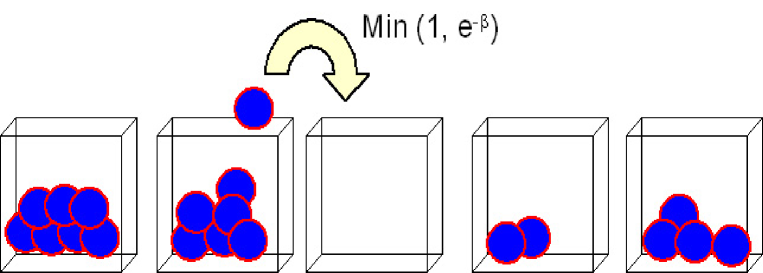
In the original formulation the model was studied under Metropolis dynamics where at each time step a particle is chosen at random and a destination box selected. The move is accepted with probability one if the energy either decreases or does not change, and with probability $\exp(-\beta)$ otherwise (see figure 1). Note that the energy can only increase by one unit at each time step. The original geometry is mean-field, so the destination box is chosen at random with uniform probability among all boxes. In this case, a complete analytical study can be done and a hierarchy of dynamical equations can be obtained for the occupation probabilities bgfelix2 .

Figure 1: (Color online) Schematic representation of the dynamics of the model. At each time step a particle is chosen at random and a destination box selected with a uniform probability among all boxes. In the original formulation, the system was studied under Metropolis dynamics.

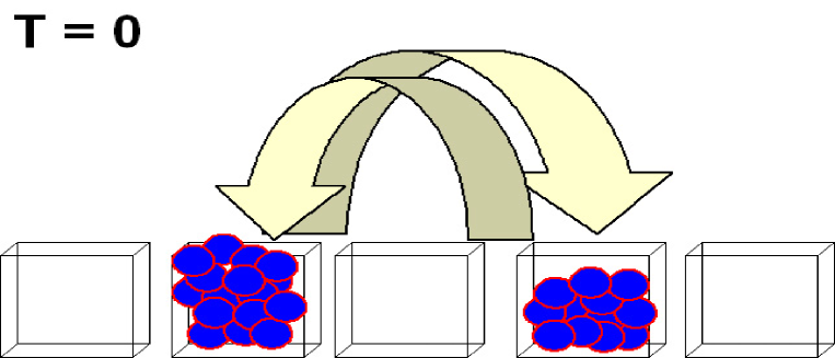
It has been shown that the dynamics is highly non trivial at very low temperatures where a dramatic slowing down of the relaxational kinetics takes place. The origin of this slowing down can be qualitatively understood. Suppose that the system starts from a configuration of high energy and the temperature is set to zero. The system will then evolve without accepting changes which increase the energy of the system. As time goes on, the system evolves towards the ground state of the system where all boxes are empty and all particles have condensed into a single box (figure 2). During the relaxation process more and more boxes are progressively emptied; this means that the few boxes which contain particles have more and more particles because the number of particles is a conserved quantity. Then, the time needed to empty an additional box increases with time. The final result is that the energy very slowly converges to the ground state value. At very low temperatures it can be shown bgfelix2 that the characteristic equilibration time is given by:

$$\tau=t_{\textrm{eq}}\simeq\frac{\exp\beta}{\beta^{2}},$$ (8)

which diverges at zero temperature. The Arrhenius dependence is remarkable if we note that only entropy barriers (but not energy barriers) are present in the model.

Figure 2: (Color online) At zero temperature only movements between occupied boxes are accepted. As time goes on, only a small fraction of boxes contain particles and the time needed to empty an additional box increases rapidly as the number of occupied boxes decreases.

The BG has been used as a playground model where new concepts of nonequilibrium thermodynamics can be tested. The fact that the dynamics is glassy and can be exactly solved has inspired several works that have investigated extensions of FDT to the nonequilibrium regime (e.g. the disordered model studied in bgleuzzi ). In the present work we solve the BG for any general Markovian dynamics and study the existence of negative FDRs.

III CORRELATIONS AND RESPONSES IN THE BG

Let us generalize the BG by adding an external field to the Hamiltonian of the model (3). The external field is introduced in order to compute the effective temperature, Eq. (1), in the nonequilibrium regime. This external field can be a local quantity (i.e. an external field acting on a single box) or a global one (i.e. an extensive field acting on all boxes) leading to different definitions of the FDRs.

Previous studies of the nonequilibrium dynamics of the BG, such as the studies carried out in bggodreche3 , have suggested that the effective temperature depends on the observable. In the studies of Ref. bggodreche3 , the Hamiltonian was perturbed by a local external field. Recently, it has been shown that local FDRs can lead to inconsistent results if finite-N corrections are not properly taken into account bgferro , pointing out the convenience of computing global FDRs.

In order to give a complete picture of the system, throughout this paper we will compute both local and global FDRs by considering local and global external fields.

III.1 Local external field

Let us consider an external field $h$ acting on a single box (e.g. box number one) that is coupled to this box only when it contains one particle:

$$H=\sum_{r=1}^{N}\,(-\delta_{n_{r},0})-h\delta_{n_{1},1}~{}.$$ (9)

Note that this subextensive perturbation does not affect the values of the occupation probabilities $P_{k}(t)=\frac{1}{N}<\sum_{r}\delta_{n_{r},k}>$ which in equilibrium are still given by eq.(6). As can be deduced from (9) we set, without loss of generality, the density of the system $\rho=1$. However, note that all the results obtained throughout the paper are valid independently on the value of the density $\rho=N/M$ whenever $\rho$ is finite in the $N\to\infty$ limit. In Appendix A a complete derivation of the dynamical equations for the probability densities of the perturbed box $P_{k}^{1}$ is carried out (see eq.(LABEL:eq:appa_1)). In what follows we will focus on the dynamical evolution of two-time quantities: local correlations and local response functions. Local correlation functions are defined as:

$$C^{loc}_{k}(t,t_{w})=\frac{1}{N}<\sum_{r}\delta_{n_{r}(t),k}\delta_{n_{r}(t_{w}),1}>~{},$$ (10)

where the sum in (10) runs over all boxes and counts the fraction of boxes that contain $k$ particles at time $t$ provided that these boxes contained one particle at previous time $t_{w}$. The brackets denote an average over dynamical trajectories of the system and over the initial conditions. The dynamical equations for these local correlations are derived in Appendix A leading to (see eq. LABEL:eq:appa_2):

$$\frac{\partial C^{loc}_{k}(t,t_{w})}{\partial t} = W(0)[-kC^{loc}_{k}+(k+1)C^{loc}_{k+1}-C^{loc}_{k}+C^{loc}_{k-1}]+$$

$$+ (W(0)-W(-1))[P_{1}(C^{loc}_{k}-C^{loc}_{k-1})+(\delta_{k,1}-\delta_{k,0})(C^{loc}_{1}(1-P_{0})+C^{loc}_{0}P_{1})]+$$

$$+ (W(0)-W(1))[P_{0}(kC^{loc}_{k}-(k+1)C^{loc}_{k+1})+(\delta_{k,0}-\delta_{k,1})(C^{loc}_{0}(1-P_{1})+C^{loc}_{1}P_{0})]~{}.$$

This expression is valid for any Markovian dynamics. $W(\Delta E)$ denotes the transition probability between two states with energy difference $\Delta E$. From now on, we consider that the dynamics obeys local detailed balance in order to ensure the convergence toward equilibrium.

Similarly, we can compute the dynamical equations for the local response function defined as the variation of the occupation probabilities for the perturbed box when the impulse field is applied at $t_{w}$:

$$R^{loc}_{k}(t,t_{w})=\left(\frac{\delta P_{k}^{1}(t)}{\delta h(t_{w})}\right)_{h(t_{w})\rightarrow 0}~{}.$$ (12)

Again, the details about the derivation can be found in the Appendix A. The result (eq.(49)) is:

$$\frac{\partial R^{loc}_{k}(t,t_{w})}{\partial t} = W(0)[-kR^{loc}_{k}+(k+1)R^{loc}_{k+1}-R^{loc}_{k}+R^{loc}_{k-1}]$$ (13)

$$+ (W(0)-W(-1))[P_{1}(R^{loc}_{k}-R^{loc}_{k-1})+(\delta_{k,1}-\delta_{k,0})(R^{loc}_{1}(1-P_{0})+R^{loc}_{0}P_{1})]$$

$$+ (W(0)-W(1))[P_{0}(kR^{loc}_{k}-(k+1)R^{loc}_{k+1})+(\delta_{k,0}-\delta_{k,1})(R^{loc}_{0}(1-P_{1})+R^{loc}_{1}P_{0})]$$

$$+ \delta(t-t_{w})S^{loc}[<P_{k}>]~{},$$

where the $\delta$-term $S^{loc}[<P_{k}>]$ is given in eq.(50). Equations (LABEL:eq:corr_loc) and (13) are the necessary ingredients for computing nonequilibrium effective temperatures.

From (LABEL:eq:corr_loc) and (13), we can check that FDT is verified at equilibrium. Indeed, at equilibrium the correlations and responses become functions of the difference of times, i.e $C^{loc}_{k}(t-t_{w})$ and $R^{loc}_{k}(t-t_{w})$ so we recover time-translational invariance. Moreover, as we can see from the form of the dynamical equations for the autocorrelations (eq.(LABEL:eq:corr_loc)) and responses (eq.(13)), at equilibrium the FDT is verified at all times provided that the initial condition for the responses (the function $S^{loc}[<P_{k}>]$) corresponds to the value of the derivative of the appropriate correlation at equal times. In this case, the correlation functions for a general observable are given by:

$$C^{loc}_{k}(t_{w},t_{w})=P_{1}(t_{w})\delta_{k,1}~{}.$$ (14)

Therefore, the initial value ($t=t_{w}$) for the derivative of the correlation functions are:

$$\left(\frac{\partial C^{loc}_{k}(t,t_{w})}{\partial t}\right)_{t\rightarrow t_{w}} = P_{1}(t_{w})\left[W(0)(-2\delta_{k,1}+\delta_{k,0}+\delta_{k,2})\right]+$$ (15)

$$+ P_{1}(t_{w})\left[W(0)-W(-1)\right](P_{1}(\delta_{k,1}+\delta_{k,2}))+$$

$$+ P_{1}(t_{w})\left[W(0)-W(-1)\right](1-P_{0})(\delta_{k,1}+\delta_{k,0})~{}.$$

Using eq.(50) it is easy to check that, in equilibrium, FDT is verified.

$$T=-\frac{\frac{\partial C^{loc}_{k}(t-t_{w})}{\partial t}}{R^{loc}_{k}(t-t_{w})}~{}.$$ (16)

III.2 Global external field

As we have explained before, local computations can lead to erroneous conclusions if finite-$N$ corrections are not properly taken into account bgferro . In such cases it is easier to carry out an analysis of FDRs for global observables. Here we shall consider the corresponding extensive perturbation of an external field coupled to the set of boxes which contain just one particle (i.e coupled to the observable $P_{1}$). The Hamiltonian reads:

$$H=-\sum_{r=1}^{N}\,(\delta_{n_{r},0}+h\delta_{n_{r},1})~{}.$$ (17)

Now, as the perturbation is extensive, all the equilibrium occupation probabilities are modified in the presence of the external field $h$:

$$P_{k}=\frac{z^{k-1}\exp(\beta\delta_{k,0}-\beta h\delta_{k,1})}{k!(e^{z}+e^{-\beta h}-1)}~{}.$$ (18)

We proceed following the same steps as in the local case. In Appendix B we have computed the dynamical equations for the occupation probabilities, eq.(LABEL:eq:appb_1), and from these equations we derive the dynamical evolution for the global correlation and response functions.

Due to the fact that the perturbation is extensive we consider the connected correlation functions:

$$C^{g}_{k}(t,t_{w})=<\gamma_{k}(t)\gamma_{1}(t_{w})>~{},$$ (19)

where

$$\gamma_{k}(t)=\frac{1}{N}\sum_{r}\delta_{n_{r},k}-P_{k}(t)~{}$$ (20)

are the deviations of the instantaneous occupation variables from their average value at a given time. The dynamical evolution for the global correlation functions is given by eq.(LABEL:eq:appb_2):

$$\frac{\partial C^{g}_{k}(t,t_{w})}{\partial t} = W(0)[-kC^{g}_{k}+(k+1)C^{g}_{k+1}-C^{g}_{k}+C^{g}_{k-1}]+$$

$$+ (W(0)-W(-1))[C^{g}_{1}(\delta_{k,1}-\delta_{k,0}+P_{k}-P_{k-1})+P_{1}(C^{g}_{k}-C^{g}_{k-1})]+$$

$$+ (W(0)-W(1))[C^{g}_{0}(kP_{k}-(k+1)P_{k+1}+\delta_{k,0}-\delta_{k,1})+P_{0}(kC^{g}_{k}-(k+1)C^{g}_{k+1})].$$

Again, these equations are valid for any Markovian dynamics. The global response function is the response of the occupation probabilities to the extensive perturbation coupled to the observable $P_{1}$:

$$R^{g}_{k}(t,t_{w})=\left(\frac{\delta P_{k}(t)}{\delta h(t_{w})}\right)_{h(t_{w})\rightarrow 0}~{}.$$ (22)

The result for the dynamical evolution is given in Appendix B, eq.(58), and it reads:

$$\frac{\partial R^{g}_{k}(t,t_{w})}{\partial t} = W(0)[-kR^{g}_{k}+(k+1)R^{g}_{k+1}-R^{g}_{k}+R^{g}_{k-1}]+$$ (23)

$$+ (W(0)-W(-1))[R^{g}_{1}(\delta_{k,1}-\delta_{k,0}+P_{k}-P_{k-1})+P_{1}(R^{g}_{k}-R^{g}_{k-1})]+$$

$$+ (W(0)-W(1))[R^{g}_{0}(kP_{k}-(k+1)P_{k+1}+\delta_{k,0}-\delta_{k,1})+P_{0}(kR^{g}_{k}-(k+1)R^{g}_{k+1})]+$$

$$+ \delta(t-t_{w})S^{g}[<P_{k}>]~{},$$

where we have introduced the function $S^{g}[<P_{k}>]$ which depends only on one time and gives the initial value for the responses. The exact form of $S^{g}[<P_{k}>]$ is given in eq. (LABEL:eq:appb_delta).

Again, we check that in equilibrium FDT is verified. Indeed, at equal times the global correlations are given by:

$$C^{g}_{k}(t_{w},t_{w})=-P_{k}(t_{w})(P_{1}(t_{w})-\delta_{k,1})~{}.$$ (24)

Obviously, in equilibrium the correlations at equal times do not depend on time. Inserting this initial value in the equations for the correlations and by considering the equilibrium case, it is easy to prove FDT for all $k$ values of the observables $C^{g}_{k}$, $R^{g}_{k}$:

$$T=-\frac{\frac{\partial C^{g}_{k}(t-t_{w})}{\partial t}}{R^{g}_{k}(t-t_{w})}~{}.$$ (25)

IV RESULTS

In this section we analyze the nonequilibrium behavior of the correlations and responses at zero temperature both for local and global observables.

The interesting glassy behavior in the BG model occurs in the zero temperature limit where entropy barriers govern the relaxational dynamics of the model. In what follows we shall consider heat-bath dynamics at zero temperature, both for the local and the global variables. This choice is motivated by the known fact that in the Metropolis algorithm there is a discontinuity of the derivative of the transition rates for $\Delta E=0$. As a result, the definition of the response functions become ambiguous, see Ref.bggodreche3 . We circumvent this drawback by employing heat bath dynamics.

IV.1 Local two-time quantities

From the numerical integration of equations (LABEL:eq:corr_loc) and (13) we can analyze the nonequilibrium behavior of the local correlations and response functions. From now on, all the numerical results shown are obtained using heat bath dynamics at zero temperature.

IV.1.1 Correlations and responses

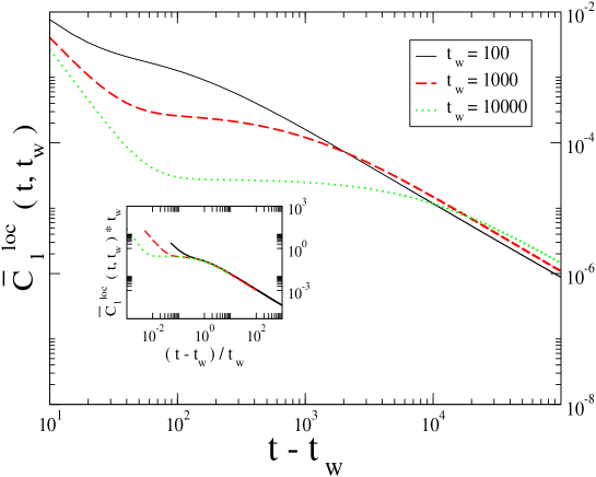
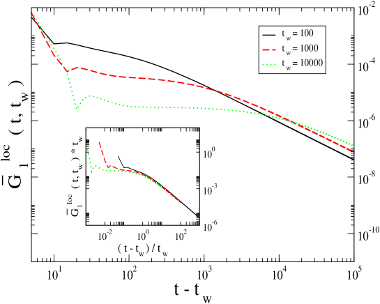
In figure 3 we plot the normalized local correlation $\bar{C}^{loc}_{1}(t,t_{w})=\frac{C_{1}(t,t_{w})}{P_{1}(t_{w})}$ at zero temperature. We can clearly see the aging effects in the local correlation function: as $t_{w}$ increases the autocorrelation function develops a plateau showing two characteristic and well separated time-scales: the first timescale corresponds to the initial relaxation of the system (usually called $\beta$-relaxation) which does not depend much on $t_{w}$; the second one is larger, increases with $t_{w}$ and corresponds to the late decay of the correlation function, usually known as $\alpha$-relaxation. The existence of these two time-scales is a typical signature of the glassy relaxation of structural glasses.

In the inset of figure 3 we plot the local normalized correlation function $\bar{C}^{loc}_{1}(t,t_{w})$ multiplied by $t_{w}$ in order to collapse all curves on the same plateau. It is clear that the system displays simple aging, i.e the scaling $t/t_{w}$ is well satisfied.

Figure 3: (Color online) The evolution for the normalized local correlation function $\bar{C}^{loc}_{1}(t,t_{w})$ (dimensionless) for different $t_{w}$’s. In the inset the scaling of $\bar{C}^{loc}_{1}(t,t_{w})$ corresponding to simple aging is displayed. The time is measured in Monte Carlo sweeps.

Regarding response functions, they show some peculiarities: on the one hand, the initial value for the response functions (given by the function $S^{loc}[<P_{k}>]$) is proportional to $\beta$, giving a divergence at zero temperature (a known common feature of kinetically constrained models sollich_negative2 ); on the other hand, the response function $R^{loc}_{1}(t,t_{w})$ is non-monotonic (for $t_{w}$ fixed when $t$ is varied) and becomes negative for long enough times. In figure 4 we plot both the local, $R^{loc}_{1}$, and the global, $R^{g}_{1}$, response functions for the observable $P_{1}$ (see below). Both responses show a non-monotonic behavior and become negative for long times.

Figure 4: (Color online) Time dependence of the global and local dimensionless response functions multiplied by $T$ ($TR^{g}_{1}$ and $TR^{loc}_{1}$) at $t_{w}=1000$. The time is measured in Monte Carlo sweeps.

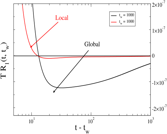
The non-monotonicity of the response function can be easily understood. The external field is coupled to $P_{1}$, therefore the system tends to increase the population of boxes with one particle; however, because boxes with one particle are bottlenecks for the relaxation of the energy, a transient increase in their number at $t_{w}$, induces a faster relaxation of the energy at later times. Because the natural evolution of the system tends to decrease $P_{1}$ when decreasing the energy, a transient increase of $P_{1}$ at $t_{w}$ causes a net decrease of the same quantity at later times when energy relaxation becomes faster.

In order to facilitate the readings of the effective temperature in our plots we introduce the function $\bar{G}^{loc}_{1}(t,t_{w})$ as:

$$\bar{G}^{loc}_{1}(t,t_{w})=T\frac{|(R^{loc}_{1}(t,t_{w}))|}{P_{1}(t_{w})}~{}~{},$$ (26)

which is the normalized absolute value of the response $R^{loc}_{1}(t,t_{w})$ multiplied by $T$. Due to the change of sign of $R^{loc}_{1}$, we have taken the absolute value in order to plot the relaxation in a log-log scale.

In figure 5 we plot $\bar{G}^{loc}_{1}(t,t_{w})$ for different values of $t_{w}$. As can be inferred from figure 5, the dip at short times corresponds to the change in sign of the response. Looking at this logarithmic plot, the response shows again the two characteristic relaxation time-scales of glasses. In the inset of figure 5 we can see that the response function also displays simple aging with scaling $t/t_{w}$ as the leading term.

Figure 5: (Color online) The evolution of the dimensionless quantity, $\bar{G}^{loc}_{1}(t,t_{w})$, (26) at different values of $t_{w}$. In the inset we show the simple aging scaling for this quantity. The dips observed in $\bar{G}^{loc}_{1}$ indicate changes of sign in $R^{loc}_{1}$. The time is measured in Monte Carlo sweeps.

It is worth noting that this simple aging relaxation in the $\alpha$-regime can also be seen in the correlations and responses for the other observable quantities of the model, i.e in the dynamical behavior of $C^{loc}_{k}(t,t_{w})$ and $R^{loc}_{k}(t,t_{w})$ for a generic $k$ (data not shown).

IV.1.2 Nonequilibrium effective temperatures

We now define a set of effective temperatures from the nonequilibrium definition, eq.(1):

$$\left(T_{\rm eff}^{loc}\right)_{k}(t,t_{w})=\frac{\frac{\partial C^{loc}_{k}(t,t_{w})}{\partial t_{w}}}{R^{loc}_{k}(t,t_{w})}~{}.$$ (27)

In order for $\left(T_{\rm eff}^{loc}\right)_{k}(t,t_{w})$ to share some of the properties of a thermometric temperature it should not asymptotically depend on the integer $k$ (for a fixed $t_{w}$ and in the large $t$ limit). In figure 6 we plot the ratio between the absolute value of the effective temperature and the physical one (in the limit $T\rightarrow 0$), which corresponds to the inverse of the local FDR kurchan defined as:

$$X^{loc}_{k}(t,t_{w})=\frac{T}{\left(T_{\rm eff}^{loc}\right)_{k}(t,t_{w})}~{}~{}~{}~{}.$$ (28)

Figure 6: (Color online) The absolute value of the effective temperature divided by $T$ for the observable $P_{1}$ ($k=1$) as a function of time for different $t_{w}$’s. The (up and down) oriented spikes indicate changes in the sign of $\left(T_{\rm eff}^{loc}\right)_{1}$. Note that, for a given $t_{w}$, the effective temperature changes sign twice. Therefore, we can distinguish three regions depending of the sign of the local FDR. The time is measured in Monte Carlo sweeps.

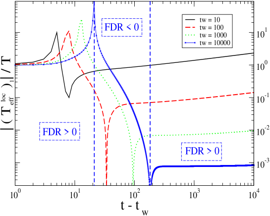
We can clearly see that the effective temperature shows two different behaviors depending on the time-scales considered. For $t\to t_{w}$ the value of the FDR converges to 1 as $t_{w}$ increases. This is a typical feature of glasses: the first $\beta$-relaxation is an equilibrium process which implies that the effective temperature is just the physical one. This is true in the asymptotic limit $t_{w}\rightarrow\infty$. It can be shown that it converges to 1 in a logarithmic way as was found in the analysis of Ref.bggodreche3 .

From the integration of the dynamical equations, we obtain the asymptotic value of the ratio $\left(T^{loc}_{\rm eff}\right)_{k}(t,t_{w})/T$, which is positive because for long enough times both the local response and the derivative of the local correlation become negative. This asymptotic value tends to zero in the limit $t_{w}\rightharpoonup\infty$. In addition, for a given waiting time the effective temperature is proportional to the bath temperature.

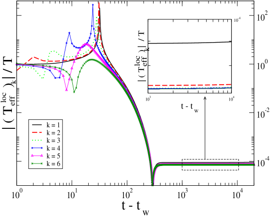
Looking at figure 7, where we plot the effective temperature at $t_{w}=10000$ for different observables, we can clearly see that the effective temperature depends on the observable under scrutinity. Consequently, it seems clear that from a local point of view we cannot define a unique effective temperature by using the FDR.

Figure 7: (Color online) The absolute value of the effective temperature divided by $T$ ($t_{w}=10000$) as a function of time for different observables $k$. In the inset we zoom the boxed part of the figure in order to emphasize the observable dependence of the effective temperature. The (up and down) oriented spikes indicate changes in the sign of $\left(T_{\rm eff}^{loc}\right)_{k}$. The time is measured in Monte Carlo sweeps.

IV.2 Global two-time quantities

In the preceding section we have shown that a unique effective temperature cannot be defined by the FDR from a local perturbation. As we have mentioned before, this is an expected result consistent with previous analysis bggodreche3 . In this section we will analyze the time dependence of the global correlation and the global response functions and we will show that a unique negative effective temperature can be defined from the global FDRs.

IV.2.1 Correlations and responses

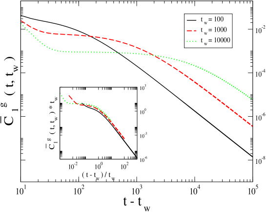
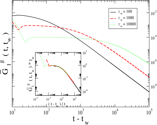
We study the connected correlation functions for heat bath dynamics of the BG at zero temperature. In Fig.8 we plot the normalized correlation function, $\bar{C}^{g}_{1}(t,t_{w})=\frac{C^{g}_{1}(t,t_{w})}{P_{1}(t_{w})}$, for different values of $t_{w}$. Similarly to the local case, we can clearly distinguish two characteristic time-scales in the system, the $\beta$-relaxation and the $\alpha$-relaxation. Note that, as $t_{w}$ increases, the plateau value of the correlation decreases and in the limit $t_{w}\to\infty$ the plateau value converges to zero. In the inset of Fig.8 we have multiplied this normalized correlation by $t_{w}$. As for the local case, the global correlation displays simple aging.

Figure 8: (Color online) The global (connected) correlation function normalized for different $t_{w}$’s. In the inset we plot the simple aging scaling for $\bar{C}^{g}_{1}(t,t_{w})$. These correlation functions are dimensionless and the time is measured in Monte Carlo sweeps.

Again, in order to analyze the relaxation of the global response function we have defined the normalized response function $\bar{G}^{g}_{1}(t,t_{w})$

$$\bar{G}^{g}_{1}(t,t_{w})=T\frac{|(R^{g}_{1}(t,t_{w}))|}{P_{1}(t_{w})},$$ (29)

motivated by the fact that the response function $R_{1}^{g}(t,t_{w})$ becomes negative for long times as it is shown in figure 4. This is again consequence of the fact that the natural evolution of the system tends to diminish $P_{1}(t_{w})$ in opposition to the action of the external field. Moreover, the global response function is proportional to the bath temperature, which diverges at zero temperature. In figure 9 we plot the two time-scales relaxation of $\bar{G}^{g}_{1}(t,t_{w})$. In the inset of figure 9 we show the simple aging scaling of the function $\bar{G}^{g}_{1}(t,t_{w})$. Again, the dip of the curves at short times corresponds to the time when the response changes its sign.

Figure 9: (Color online) The global scaled response function for $P_{1}$ for different $t_{w}$’s. The dips observed in $\bar{G}^{g}_{1}$ (dimensionless) indicate changes in the sign of $R^{g}_{1}$. The time is measured in Monte Carlo sweeps.

The global correlations and responses for the rest of the observables in the model, $\bar{C}_{k}^{g}(t,t_{w})$ and $\bar{G}_{k}^{g}(t,t_{w})$, also display simple aging (data not shown). It is worth mentioning that the ratio between $\bar{C}_{k}^{g}$ and $\bar{G}_{k}^{g}$ for $k>1$ is of the same order of magnitude as the one corresponding to $k=1$.

IV.2.2 Nonequilibrium effective temperatures

As we have done for local observables, from the FDR we can define the effective temperatures:

$$\left(T_{\rm eff}^{g}\right)_{k}(t,t_{w})=\frac{\frac{\partial C^{g}_{k}(t,t_{w})}{\partial t_{w}}}{R^{g}_{k}(t,t_{w})}~{}.$$ (30)

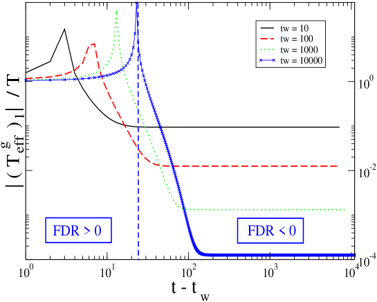
In figure 10 we plot the absolute value of the effective temperature $\left(T^{g}_{\rm eff}\right)_{1}(t,t_{w})$ divided by $T$ for different values of $t_{w}$. This quantity is related to the global FDR $X^{g}_{1}(t_{w})$ for $P_{1}$ as:

$$X^{g}_{1}(t_{w})=\frac{T}{\left(T^{g}_{\rm eff}\right)_{1}(t,t_{w})}~{}~{},$$ (31)

As in the local case, the value of $\frac{\left(T^{g}_{\rm eff}\right)_{1}(t,t_{w})}{T}$ in the limit $t\to t_{w}$ tends to 1 showing that the first $\beta$-regime corresponds to an equilibrium relaxation process (i.e $X^{g}_{1}=1$). We can also see that, in contrast with the local case, this global effective temperature remains constant throughout the $\alpha$-regime for any finite $t_{w}$.

Figure 10: (Color online) The absolute value of the global effective temperature function normalized by $T$ for $P_{1}$ for different values of $t_{w}$. The up oriented spikes indicate changes in the sign of $\left(T_{\rm eff}^{g}\right)_{1}$ which is negative for long times. The time is measured in Monte Carlo sweeps.

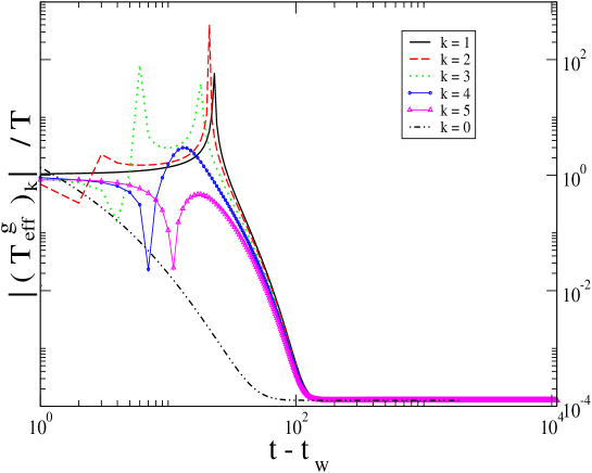
A very important aspect of the global effective temperature is the fact that, for a given value of the waiting time this effective temperature does not depend on the observable as can be seen in figure 11 where we have plotted the absolute value of the inverse of the global FDRs (eq.(31)) at $t_{w}=10000$ for different observables. It is clear that the asymptotic value of the FDRs at finite $t_{w}$ does not depend on the observable.

Figure 11: (Color online) The global effective temperature function normalized by $T$ for $tw=10000$ and for different observables. The (up and down) oriented spikes indicate changes in the sign of $\left(T_{\rm eff}^{g}\right)_{k}$. Note that for some values of $k$ the effective temperature changes sign more than twice. The time is measured in Monte Carlo sweeps.

Moreover, from the results of figure 10 we can see that for large waiting times $t_{w}$ the inverse of the FDR scales as the inverse of $t_{w}$:

$$\frac{\left(T^{g}_{\rm eff}\right)_{k}(t,t_{w})}{T}=\frac{1}{X^{g}_{k}(t_{w})}\simeq-\frac{1}{t_{w}}~{}~{}~{}~{}\forall~{}k~{}.$$ (32)

Again, the minus sign in eq.(32) is a consequence of the non-monotonicity of the response functions. Finally, it is worth mentioning that we have checked that all the results obtained at zero temperature throughout this paper remain valid at finite but very low temperatures. The analysis at finite small temperatures does not give new insights into the nonequilibrium behavior of the system as all dynamical quantities smoothly converge to their $T=0$ limit.

IV.3 Asymptotic analysis

In the preceding section we have obtained a negative FDR independent of the observable that displays simple scaling of the type $t/t_{w}$. This result can be easily understood by analyzing the asymptotic nonequilibrium relaxation of the model. The equilibrium probabilities in the presence of an external field are given by:

$$P_{k}=\frac{z^{k-1}\exp(\beta(\delta_{k,0}-h\delta_{k,1})}{k!\exp(z)}.$$ (33)

In the long time asymptotic regime, the multiplier $z(t)$ is a function of time which grows as bgfelix3 ; bgfelix4 :

$$z(t)\approx{\rm ln}t+{\rm ln}({\rm ln}t)~{}~{}.$$ (34)

With the global perturbation considered along the paper we can compute the global susceptibility $\chi^{g}_{1}$ by assuming local equilibrium using (18) with $k=1$:

$$T\chi^{g}_{1}=T\lim_{h\rightarrow 0}\frac{P_{1}(h=0)-P_{1}(h)}{h}=\frac{1}{e^{z}}~{}~{}.$$ (35)

From (34) the global susceptibility associated to the observable $P_{1}(t)$ decays as:

$$T\chi^{g}_{1}(\tau)=\frac{1}{\tau{\rm ln}\tau}~{}~{},$$ (36)

where $\tau=t-t_{w}$. The asymptotic decay of $R^{g}_{1}(\tau)$ is given by the derivative of $\chi^{g}_{1}(\tau)$ multiplied by the temperature:

$$TR^{g}_{1}(\tau)=-\frac{1}{\tau^{2}{\rm ln}\tau}+{\cal{O}}\left(\frac{1}{\tau^{2}{\rm ln}^{2}\tau}\right)~{}~{}.$$ (37)

Now, by using the equation (23) at zero temperature:

$$\frac{\partial R_{0}^{g}}{\partial\tau}=R^{g}_{1}-P_{0}R_{1}^{g}-P_{1}R_{0}^{g}~{}~{}~{}~{},$$ (38)

we obtain the asymptotic decay of $R^{g}_{0}$:

$$TR^{g}_{0}(\tau)=\frac{1}{\tau{\rm ln}^{2}\tau}+{\cal{O}}\left(\frac{1}{\tau^{2}{\rm ln}^{3}\tau}\right)~{}~{}.$$ (39)

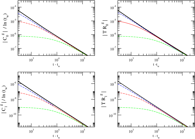
In the right column of figure 12 we numerically confirm the scalings (37) and (39) for different values of $t_{w}$. Due to the fact that the dynamical equations for the correlations are formally identical to those for the response functions one finds:

$$C^{g}_{0}(\tau,t_{w}) = -\frac{{\rm ln}(t_{w})}{\tau{\rm ln}^{2}\tau}+{\cal{O}}\left(\frac{1}{\tau^{2}{\rm ln}^{3}\tau}\right)$$

$$C^{g}_{1}(\tau,t_{w}) = \frac{{\rm ln}(t_{w})}{\tau^{2}{\rm ln}\tau}+{\cal{O}}\left(\frac{1}{\tau^{2}{\rm ln}^{2}\tau}\right)~{}~{},$$ (40)

where the dependence on $t_{w}$ has been inferred from the decay of the global correlations at equal times (eq.(24)).

These scalings are again confirmed numerically and are shown in the left column of figure 12. With these scalings we recover the following FDRs:

$$X^{g}_{0}(t_{w})=X^{g}_{1}(t_{w})\simeq-t_{w}~{}~{},$$ (41)

in agreement with our numerical findings. A similar analysis can be done for $k>1$.

Figure 12: (Color online) Left column: scaling of the global correlations $C^{g}_{0}$ and $C^{g}_{1}$ divided by ${\rm ln}(t_{w})$. Right column: scaling of the global correlations $R^{g}_{0}$ and $R^{g}_{1}$ multiplied by $T$. The continuous lines are the assymptotic scalings (40) and (39), (37) while the discontinuous lines correspond, from top to bottom, to $t_{w}$= 100, 1000, 10000 respectively. All quantities are dimensionless and the time is measured in Monte Carlo sweeps.

V CONCLUSIONS

In this paper we have solved the relaxation of the correlations and response functions in the BG model for a general dynamic rule (provided that it satisfies local detailed balance). We have studied (by means of numerical integration and analytic asymptotic expansions) the behavior of effective temperatures and FDRs in the glassy regime.

We have found that both the correlation and the response functions show two characteristic time-scales: a first $\beta$-relaxation for short times characterized by an equilibrium FDR, $X(t,t_{w})=1$, and a second $\alpha$-relaxation at long times with a non-trivial value of the FDR. This is a very common feature of structural glasses and other glassy systems. Moreover, we have found that both the correlations and responses display simple aging.

In this paper we have analyzed the resulting FDRs obtained from local and global perturbations. The interesting conclusion is that the local FDRs depend on both $t$ and $t_{w}$ while the global FDRs only depends on $t_{w}$. Moreover, global FDRs are independent of the observable in contrast with the local ones.

More interesting is the fact that this observable-independent value of the global FDR is negative and diverges with the waiting time as:

$$X^{g}(t_{w})\approx-t_{w}~{}~{}~{}.$$ (42)

This result points in the same direction as recent studies on kinetically constrained models sollich_negative ; sollich_negative2 which also found negative FDRs. In these studies, the negative character of the FRDs was associated to activation effects in the dynamics. In the present case, we have found negative FDRs in the sole presence of entropic barriers for the BG.

It is worth emphasizing that negative FDRs are related to non-monotonic response functions. In the glassy literature, non-monotonic responses are associated with non-neutral observable quantities bgreviewcris . The non-neutrality property of these observables emerges as a consequence of the dynamic coupling between the external field and the energy of the system leading to negative effective temperatures.

In this paper we showed that an observable-independent FDR can be properly defined by studying global observables. However, we found a unique negative FDR due to the non-neutrality of the observables under scrutinity. Therefore, the neutrality of an observable seems to be a key aspect in order to define nonequilibrium effective temperatures.

How much current results would change if the perturbation $h\delta_{n,k}$ acts along an arbitrary direction $k>1$? We do not expect big qualitative changes in our results depending on the ”orientation” of the field provided that $k$ is finite (and $k<<N$). Arbitrary values of $k$ will result in a bottleneck effect similar to that observed in the current study for $k=1$. However, for $k/N$ finite the bottleneck effect will be substantially different because the energy will not be able to reach the asymptotic low energy regime $E\to-1+\frac{1}{{\rm ln}(t)}~{}.$

Finally, it would be extremely helpful to find a microcanonical derivation or a phenomenological argument for reproducing the asymptotic behavior of the effective temperature when perturbing along arbitrary observables $P_{k}$. This could be done either by a closure of the dynamical equations by using a partial equilibration hypothesis, or by exact computation of the appropriate configurational entropy in the off-equilibrium regime. Such arguments would greatly facilitate the computation of effective temperatures without having to solve the full set of dynamical equations for correlations and responses.

Acknowledgments

A.G. wish to thank CEAV for its support during the last stages of this work. F.R. acknowledges support from the Spanish and Catalan Research Councils from grants FIS2007-61433, NAN2004-9348, SGR05-00688. I.P. acknowledges support from the Spanish and Catalan Research Councils from grants FIS2005-01299 and SGR05-00236.

Appendix A Local dynamical equations

In the present analysis we consider a general dynamics with just one restriction: it must obey local detailed balance. This restriction ensures that the system converges to its equilibrium state. In fact, we will see that this is the necessary condition for FDT to be obeyed at equilibrium. From now on, the transition probabilities will be expressed by $W(\Delta E)$ where $\Delta E$ is the energy difference between the final and the initial states.

A.0.1 One-time quantities.

The dynamic equations for the occupation probabilities can be computed in the same way as have been obtained for the Monte-Carlo dynamics of this model (see Ref.bgfelix3 for details). The general result is:

$$\frac{\partial P^{1}_{k}}{\partial t} = W(0)[-kP^{1}_{k}+(k+1)P^{1}_{k+1}-P^{1}_{k}+P^{1}_{k-1}]+$$

$$+ (W(0)-W(-1+h))[P^{1}_{1}(1-P_{0})(\delta_{k,1}-\delta_{k,0})+P^{1}_{1}P_{1}(\delta_{k,1}-\delta_{k,2})]+$$

$$+ (W(0)-W(h))[P^{1}_{1}P_{0}(\delta_{k,1}-\delta_{k,0})+P^{1}_{1}(1-P_{1})(\delta_{k,1}-\delta_{k,2})]+$$

$$+ (W(0)-W(-h))[2P^{1}_{2}(1-P_{0})(\delta_{k,2}-\delta_{k,1})+P^{1}_{0}P_{1}(\delta_{k,0}-\delta_{k,1})]+$$

$$+ (W(0)-W(1-h))[2P^{1}_{2}P_{0}(\delta_{k,2}-\delta_{k,1})+P^{1}_{0}(1-P_{1})(\delta_{k,0}-\delta_{k,1})]+$$

$$+ (W(0)-W(1))[P_{0}(kP^{1}_{k}-(k+1)P^{1}_{k+1})+P^{1}_{1}P_{0}(\delta_{k,0}-\delta_{k,1})+2P^{1}_{2}P_{0}(\delta_{k,1}-\delta_{k,2})]+$$

$$+ (W(0)-W(-1))[P_{1}(P^{1}_{k}-P^{1}_{k-1})+P^{1}_{0}P_{1}(\delta_{k,1}-\delta_{k,0})+P^{1}_{1}P_{1}(\delta_{k,2}-\delta_{k,1})]~{}~{}.$$

The quantities $P_{k}(t)$ are the occupation probabilities, while the quantities $P^{1}_{k}(t)$ are the average occupation probabilities restricted to the box number one, which is the box affected by the external field. As a particular case we can get the dynamic evolution for the occupation probabilities for any box at zero field:

$$\frac{\partial P_{k}}{\partial t} = W(0)[-kP_{k}+(k+1)P_{k+1}-P_{k}+P_{k-1}]+$$ (44)

$$+ (W(0)-W(-1))[P_{1}(P_{k}-P_{k-1}+\delta_{k,1}-\delta_{k,0})]+$$

$$+ (W(0)-W(1))[P_{0}(kP_{k}-(k+1)P_{k+1}+\delta_{k,0}-\delta_{k,1}]~{}~{}.$$

These equations cannot be solved exactly (although an analytic treatment has been done in the asymptotic regime bgfelix3 ) but can be integrated numerically to give the full solution. More significative, these equations are the first step in order to compute the dynamical evolution of two-time quantities such as the autocorrelation functions and the local response functions.

A.0.2 Local correlations and response functions

As a consequence of the local character of the external field, we have to deal with the corresponding local response functions and the box-box autocorrelation functions. These autocorrelation functions are defined as follows:

$$C^{loc}_{k}(t,t_{w})=\frac{1}{N}<\sum_{r}\delta_{n_{r}(t),k}\delta_{n_{r}(t_{w}),1}>~{},$$ (45)

which can be expressed in terms of the following conditional probabilities $\nu_{k}(t,t_{w})=P(n_{r}(t)=k|n_{r}(t_{w})=0)$:

$$C^{loc}_{k}(t,t_{w})=P_{1}(t_{w})\nu_{k}(t,t_{w})~{}.$$ (46)

Following the same strategy as in bgfelix3 the dynamic equations for these conditional probabilities give:

$$\frac{\partial\nu_{k}(t,t_{w})}{\partial t} = W(0)[-k\nu_{k}+(k+1)\nu_{k+1}-\nu_{k}+\nu_{k-1}]+$$

$$+ (W(0)-W(-1))[P_{1}(\nu_{k}-\nu_{k-1})+(\delta_{k,1}-\delta_{k,0})(\nu_{1}(1-P_{0})+\nu_{0}P_{1})]+$$

$$+ (W(0)-W(1))[P_{0}(k\nu_{k}-(k+1)\nu_{k+1})+(\delta_{k,0}-\delta_{k,1})(\nu_{0}(1-P_{1})+\nu_{1}P_{0})]~{}.$$

The corresponding local response functions are just the variations of the occupation probabilities for the perturbed box with the external field:

$$R^{loc}_{k}=\left(\frac{\delta P_{k}^{1}(t)}{\delta h(t_{w})}\right)_{h(t_{w})\rightarrow 0}~{}.$$ (48)

From this expression and eq.(44) we arrive at:

$$\frac{\partial R^{loc}_{k}(t,t_{w})}{\partial t} = W(0)[-kR^{loc}_{k}+(k+1)R^{loc}_{k+1}-R^{loc}_{k}+R^{loc}_{k-1}]$$ (49)

$$+ (W(0)-W(-1))[P_{1}(R^{loc}_{k}-R^{loc}_{k-1})+(\delta_{k,1}-\delta_{k,0})(R^{loc}_{1}(1-P_{0})+R^{loc}_{0}P_{1})]$$

$$+ (W(0)-W(1))[P_{0}(kR^{loc}_{k}-(k+1)R^{loc}_{k+1})+(\delta_{k,0}-\delta_{k,1})(R^{loc}_{0}(1-P_{1})+R^{loc}_{1}P_{0})]$$

$$+ \delta(t-t_{w})S^{loc}[<P_{k}>]$$

Note that formally, the dynamic evolution for the response functions is just the same as for the autocorrelation functions. This is a general feature and is due to the fact that in equilibrium FDT must be satisfied. The only difference is that in the equation for the responses there is a delta term which fixes the value for $R^{loc}_{k}(t_{w},t_{w})$. This term comes from the first order of the Taylor expansion in the transition probabilities which depend on the external field $h$. This is not an approximation because higher order terms in Taylor’s expansion vanish when we set the external field equal to zero. The function $S^{loc}[<P_{k}>]$ is defined as:

$$S^{loc}[<P_{k}>] = \beta e^{\beta}W(1)[P_{1}(1-P_{0})(\delta_{k,1}-\delta_{k,0})+P_{1}^{2}(\delta_{k,1}-\delta_{k,2})]+$$ (50)

$$+ \beta e^{\beta}W^{\prime}(1)[P_{1}(1-P_{0})(\delta_{k,1}-\delta_{k,0})+P_{1}^{2}(\delta_{k,1}-\delta_{k,2})]-$$

$$- \beta W(0)[2P_{2}(1-P_{0})(\delta_{k,2}-\delta_{k,1})+P_{1}P_{0}(\delta_{k,0}-\delta_{k,1})]-$$

$$- \beta W^{\prime}(0)[2P_{2}(1-P_{0})(\delta_{k,2}-\delta_{k,1})]+$$

$$+ \beta W^{\prime}(1)[2P_{2}P_{0}(\delta_{k,2}-\delta_{k,1})+(1-P_{1})P_{0}(\delta_{k,0}-\delta_{k,1})]-$$

$$- \beta W^{\prime}(0)[(1-P_{1})P_{0}(\delta_{k,0}-\delta_{k,1})]~{},$$

where W’ denotes the derivative of the transition probability with respect to $\Delta E$. Finally, we must stress that in this equation we have already supposed that our dynamics verifies local detailed balance. If W’ is discontinuous we should have to consider two possible response functions depending on the chosen value for W’ bggodreche3 .

Appendix B Global dynamical equations

As we have made in the case of a local perturbation, we consider a general dynamics with the only condition that it must obey detailed balance. As before, this is the unique ingredient we need to ensure that equilibrium is reached at long enough times.

B.0.1 One-time quantities.

By considering all the possible elementary moves, we get the following dynamical equations for the occupation probabilities:

$$\frac{\partial P_{k}}{\partial t} = W(0)[-kP_{k}+(k+1)P_{k+1}-P_{k}+P_{k-1}]+$$

$$+ (W(0)-W(h-1))[P_{1}(1-P_{1})(\delta_{k,1}-\delta_{k,0})+P_{k}P_{1}(1-\delta_{k,1})-P_{k-1}P_{1}(1-\delta_{k,2})]+$$

$$+ (W(0)-W(2h-1))[P_{1}^{2}(2\delta_{k,1}-\delta_{k,0}-\delta_{k,2})]+$$

$$+ (W(0)-W(-h))[2P_{2}(1-P_{0})(\delta_{k,2}-\delta_{k,1})+2P_{k}P_{2}(1-\delta_{k,0})-2P_{k-1}P_{2}(1-\delta_{k,1})]$$

$$+ (W(0)-W(1-2h))[-2P_{0}P_{2}(2\delta_{k,1}-\delta_{k,0}-\delta_{k,2})]+$$

$$+ (W(0)-W(1-h))[P_{0}(kP_{k}-(k+1)P_{k+1}+\delta_{k,0}-\delta_{k,1}+2P_{2}(2\delta_{k,1}-\delta_{k,0}-\delta_{k,2}))]$$

$$+ (W(0)-W(h))[P_{1}(kP_{k}-(k+1)P_{k+1}+\delta_{k,1}-\delta_{k,2})+P_{1}^{2}(-2\delta_{k,1}+\delta_{k,0}+\delta_{k,2})]~{}.$$

Note that now, due to the global character of the field, we have to consider only the occupation probabilities averaged over the whole system. As we expect, at zero field we recover the same equations as in the local case (which are the extension of the equations obtained for Monte Carlo dynamics bgfelix2 ):

$$\frac{\partial P_{k}}{\partial t} = W(0)[-kP_{k}+(k+1)P_{k+1}-P_{k}+P_{k-1}]+$$ (52)

$$+ (W(0)-W(-1))[P_{1}(\delta_{k,1}-\delta_{k,0}+P_{k}-P_{k-1})]+$$

$$+ (W(0)-W(1))[P_{0}(kP_{k}-(k+1)P_{k+1}+\delta_{k,0}-\delta_{k,1})]~{}.$$

These equations are the first step in order to compute the dynamical equations for the correlation and response functions and give the evolution of all the possible observable physical quantities of this model. Moreover, these equations are the base of the more complex computations of the dynamical evolution of the two-time correlation and response functions.

B.0.2 Global correlations and response functions

Due to the extensive nature of the perturbation the correlation functions related with the responses are the connected ones. So, let us introduce the deviation of the instantaneous values of the occupations from their average value at each time:

$$\gamma_{k}(t)=\frac{1}{N}\sum_{r}\delta_{n_{r},k}-P_{k}(t)~{},$$ (53)

These quantities will give us insight on the fluctuations of the occupation numbers (i.e the correlations). The dynamical evolution of these quantities is:

$$\frac{\partial\gamma_{k}}{\partial t} = W(0)[-k\gamma_{k}+(k+1)\gamma_{k+1}-\gamma_{k}+\gamma_{k-1}]+$$

$$+ (W(0)-W(-1))[\gamma_{1}(\delta_{k,1}-\delta_{k,0}+P_{k}-P_{k-1})+P_{1}(\gamma_{k}-\gamma_{k-1})]+$$

$$+ (W(0)-W(1))[\gamma_{0}(kP_{k}-(k+1)P_{k+1}+\delta_{k,0}-\delta_{k,1})+P_{0}(k\gamma_{k}-(k+1)\gamma_{k+1})].$$

In this equation we have considered that the quantities $\gamma_{k}$ are of order $1/N$, so we have neglected the quadratic terms $\gamma_{k}\gamma_{l}$ in these equations because they vanish in the thermodynamic limit. The global connected correlation function will be:

$$C^{g}_{k}(t,t_{w})=<\gamma_{k}(t)\gamma_{1}(t_{w})>~{}.$$ (55)

The equations of motion for these correlations are easy to compute from these equations and give:

$$\frac{\partial C^{g}_{k}(t,t_{w})}{\partial t} = W(0)[-kC^{g}_{k}+(k+1)C^{g}_{k+1}-C^{g}_{k}+C^{g}_{k-1}]+$$

$$+ (W(0)-W(-1))[C^{g}_{1}(\delta_{k,1}-\delta_{k,0}+P_{k}-P_{k-1})+P_{1}(C^{g}_{k}-C^{g}_{k-1})]+$$

$$+ (W(0)-W(1))[C^{g}_{0}(kP_{k}-(k+1)P_{k+1}+\delta_{k,0}-\delta_{k,1})+P_{0}(kC^{g}_{k}-(k+1)C^{g}_{k+1})].$$

Now we define the global response function (which is related to the experimental susceptibility) as the response of the probabilities to the extensive perturbation coupled to $P_{1}$:

$$R^{g}_{k}(t,t_{w})=\left(\frac{\delta P_{k}(t)}{\delta h(t_{w})}\right)_{h(t_{w})\rightarrow 0}~{}.$$ (57)

From the equations in a field and expanding to first order in $h$ we have for the response functions:

$$\frac{\partial R^{g}_{k}(t,t_{w})}{\partial t} = W(0)[-kR^{g}_{k}+(k+1)R^{g}_{k+1}-R^{g}_{k}+R^{g}_{k-1}]+$$ (58)

$$+ (W(0)-W(-1))[R^{g}_{1}(\delta_{k,1}-\delta_{k,0}+P_{k}-P_{k-1})+P_{1}(R^{g}_{k}-R^{g}_{k-1})]+$$

$$+ (W(0)-W(1))[R^{g}_{0}(kP_{k}-(k+1)P_{k+1}+\delta_{k,0}-\delta_{k,1})+P_{0}(kR^{g}_{k}-(k+1)R^{g}_{k+1})]+$$

$$+ \delta(t-t_{w})S^{g}[<P_{k}>]~{},$$

where we have defined the function $S^{g}[<P_{k}>]$ which depends only on one time and gives the initial value for the responses. Similar computations as we have done for the local case lead to:

$$S^{g}[<P_{k}>] = \beta e^{\beta}W(1)[P_{1}(1-P_{1})(\delta_{k,1}-\delta_{k,0})+P_{k}P_{1}(1-\delta_{k,1})+P_{k-1}P_{1}(1-\delta_{k,2})]+$$

$$+ \beta e^{\beta}W^{\prime}(1)[P_{1}(1-P_{1})(\delta_{k,1}-\delta_{k,0})+P_{k}P_{1}(1-\delta_{k,1})+P_{k-1}P_{1}(1-\delta_{k,2})]+$$

$$+ 2\beta e^{\beta}(W(1)+W^{\prime}(1))[P_{1}^{2}(2\delta_{k,1}-\delta_{k,0}-\delta_{k,2})]-$$

$$- \beta W(0)[2P_{2}(1-P_{0})(\delta_{k,2}-\delta_{k,1})+2P_{k}P_{2}(1-\delta_{k,0})-2P_{k-1}P_{2}(1-\delta_{k,1})]-$$

$$- \beta W^{\prime}(0)[2P_{2}(1-P_{0})(\delta_{k,2}-\delta_{k,1})+2P_{k}P_{2}(1-\delta_{k,0})-2P_{k-1}P_{2}(1-\delta_{k,1})]+$$

$$+ 2\beta W^{\prime}(1)[-2P_{0}P_{2}(2\delta_{k,1}-\delta_{k,0}-\delta_{k,2})]+$$

$$+ \beta W^{\prime}(1)[P_{0}(kP_{k}-(k+1)P_{k+1}+\delta_{k,0}-\delta_{k,1})+2P_{0}P_{2}(2\delta_{k,1}-\delta_{k,0}-\delta_{k,2})]-$$

$$- \beta W^{\prime}(0)[P_{1}(kP_{k}-(k+1)P_{k+1}+\delta_{k,1}-\delta_{k,2})+P_{1}^{2}(-2\delta_{k,1}+\delta_{k,0}+\delta_{k,2})].$$

As before $W^{\prime}(\Delta E)$ is the derivative of the transition probability with respect to $\Delta E$ evaluated at $\Delta E=0,~{}1$.

References

- (1) J. Casas-vázquez and D. Jou. Temperature in nonequilibrium states: a review of open problems and current proposals. Rep. Prog. Phys. 66 1937-2023, (2003).
- (2) Sping Glasses and Random Fields, edited by A.P. Young (World Scientific, Singapore, 1998).
- (3) R.Kubo, Repr. Progr. Phys 29 255, 1966.; R. Kubo, M. Toda and N. Hashitsume, Statistical Physics II (2nd edn. Springer Verlag, Berlin, 1991).
- (4) L.F. Cugliandolo, J. Kurchan, and L. Peliti. Energy flow, partial equilibration and effective temperatures in systems with slow dynamics. Phys. Rev. E, 55(4):3898–3914, (1997).
- (5) A. Crisanti and F. Ritort. Violations of the fluctuation-dissipation theorem in glassy systems: basic notions and the numerical evidence. J. Phys. A (Math. Gen) 36 R181, 2003.
- (6) P. Mayer, L. Berthier, J.P. Garrahan and P. Sollich. Fluctuation-dissipation relations in the nonequilibrium critical dynamics of Ising models.Physical Review E, 68 016116, 2003.
- (7) P. Mayer, S. Léonard, L. Berthier, J.P. Garrahan and P. Sollich. Activated aging dynamics and negative fluctuation-dissipation ratios. Phys. Rev. Lett. 96, 030602 (2006).
- (8) S. Léonard, P. Mayer, P. Sollich, L. Berthier and J.P. Garrahan. Nonequilibrium dynamics of spin facilitated glass models. J. Stat. Mech. P07017 (2007).
- (9) F. Ritort. Glassiness in a model without energy barriers. Physical Review Letters, 75 1190, 1995.
- (10) S. Franz and F. Ritort. Dynamical solution of a model without energy barriers.Europhysics Letters, 31 507, 1995.
- (11) S. Franz and F. Ritort. Glassy mean-field dynamics of the backgammon model. Journal of Statistical Physics, 85 131, 1996
- (12) S. Franz and F. Ritort. Relaxation processes and entropic traps in the backgammon model. Journal of Physics A, 30 L359, 1997.
- (13) C. Godreche, J.P. Bouchaud and M. Mezard. Entropy barriers and slow relaxation in some random walk models. Journal of Physics A, 28 L603, 1995.
- (14) C. Godreche and J.M. Luck. Long-time regime and scaling of correlations in a simple model with glassy behavior. Journal of Physics A, 29 1915, 1996.
- (15) C. Godreche and J.M. Luck. Correlation and response in the Backgammon model: the Ehrenfest legacy. Journal of Physics A, 32 6033, 1999.
- (16) A. Prados, J.J. Brey and B. Sanchez-Rey. Glassy behavior in a simple model with entropy barriers. Physical Review B, 55 6343, 1997.
- (17) P. Sollich and F. Ritort. Glassy dynamics of kinetically constrained models. Advances in Physics, 52 219, 2003.
- (18) P. Ehrenfest and T. Ehrenfest. The conceptual foundations of the statistical approach to mechanics. Dover, 1990.
- (19) P. Ehrenfest and T. Ehrenfest. Phys. Zeit. 8 311, 1907.
- (20) C. Godreche and J.M. Luck. Nonequilibrium dynamics of urn models. J. Phys. Cond. Matt., 14 1601, 2002.
- (21) L. Leuzzi and Th. M Nieuwenhuizen. Thermodynamics of the Glassy State. Taylor and Francis (2007).
- (22) L. Leuzzi and F. Ritort. Disordered Backgammon Model. Physical Review E, 65 56125, 2002.
- (23) A. Garriga, P. Sollich, I. Pagonabarraga and F. Ritort. Universality of Fluctuation-Dissipation Relations. The Ferromagnetic Model. Physical Review E, 72 056114, 2005.