The Gauss-Legendre Sky Pixelization for the CMB polarization (GLESP-pol). Errors due to pixelization of the CMB sky

Andrei G. Doroshkevich Astro Space Center of Lebedev Physical Institute, Profsoyuznaya 84/32, Moscow, Russia, dorr@asc.rssi.ru    Oleg V. Verkhodanov Special Astrophysical Observatory, Nizhnij Arkhyz, Karachaj-Cherkesia, 369167, Russia, vo@sao.ru    Pavel D. Naselsky Niels Bohr Institute, Blegdamsvej 17, DK-2100 Copenhagen, Denmark, naselsky@nbi.dk    Jaiseung Kim Niels Bohr Institute, Blegdamsvej 17, DK-2100 Copenhagen, Denmark, jkim@nbi.dk    Dmitry I. Novikov Imperial College, London, United Kingdom,
Astro Space Center of Lebedev Physical Institute, Profsoyuznaya 84/32, Moscow, Russia, d.novikov@imperial.ac.uk
   Viktor I. Turchaninov Keldysh Institute of Applied Math, Russian Academy of Science, Moscow, 125047, Russia    Igor D. Novikov Astro Space Center of Lebedev Physical Institute, Profsoyuznaya 84/32, Moscow, Russia,
Niels Bohr Institute, Blegdamsvej 17, DK-2100 Copenhagen, Denmark,
Niels Bohr International Academy, Blegdamsvej 17, DK-2100 Copenhagen, Denmark, novikov@asc.rssi.ru
   Lung-Yih Chiang Institute of Astronomy and Astrophysics, Academia Sinica, P.O.Box 23-141, Taipei 10617, Taiwan, Republic of China, lychiang@asiaa.sinica.edu.tw    Martin Hansen Niels Bohr Institute, Blegdamsvej 17, DK-2100 Copenhagen, Denmark
(Accepted 2009 ???? ???; Received 2009 ???? ???)
Abstract

We present developing of method of the numerical analysis of polarization in the Gauss–Legendre Sky Pixelization (GLESP) scheme for the CMB maps. This incorporation of the polarization transforms in the pixelization scheme GLESP completes the creation of our new method for the numerical analysis of CMB maps. The comparison of GLESP and HEALPix calculations is done.

1 Introduction

The analysis of the anisotropy of CMB temperature and polarization is one of the most effective methods for the extraction of the cosmological information and for tests of cosmology and fundamental physics.

The measurements of the anisotropy of CMB temperature performed by the WMAP mission allow us to establish parameters of the cosmological model of the Universe with unprecedented precision Refs. \refcitehinshaw2007, \refcitehinshaw2009, \refcitespergel2007, \refcitenolta2009.

Increasing sensitivity and angular resolution of the CMB data, including recently available WMAP 5 year data Ref. \refcitehinshaw2009 , ACBAR Ref. \refciteacbar QUaD Refs. \refcitequad1,\refcitequad2,stimulates significant development and increasing predictability of the corresponding software (see, for instance, CAMB Ref. \refcitecamb, COSMOMC Ref. \refcitecosmomc, RICO Ref. \refciterico, etc.)

During the next decade, after the PLANCK experiment, an investigation of the CMB polarization (including the B-mode) will be at the focus of the CMB science. Planning the CMBpol mission Ref. \refciteCMBpol, B-pol mission Ref. \refciteBpol, etc. requires significant improvement in estimation of the errors of the signal. Partially an uncertainties due to pixelization of the CMB sky and their propogation to the CMB power and the map can be potential sources of the error. For planning high resolution the CMB experiments the most frequently used the HEALPix package Ref. \refcitehpix as well as GLESP Ref. \refciteglesp, ECP Ref. \refciteecp, and some others, needs to be tested in order to provide an exact information about the error bars of the convolution of the T,E,B𝑇𝐸𝐵T,E,B-maps to the corresponding coefficients of the spherical harmonics decomposition not only for the power spectrum, but for the real and imaginary part of the coefficients as well.

The information about the multipole structure of the CMB signal is vital for the low multipoles (=2,3..23\ell=2,3..), since a lot of theoretical predictions about the properties of the cosmological model are related directly to the global morphology of the signal. As an example, we would like to mention widely discussed the Bianchi VIIh𝑉𝐼subscript𝐼VII_{h} anisotropic cosmological model Refs. \refciteeriksenasym, \refcitejaffebianchi, \refcitebridges which can mimic the anisotropy of the CMB power at the range of multipoles 2020\ell\leq 20, and the Cold Spot Ref. \refcitecruz as well. The whole sky decomposition is vital for testing the alignment and planarity of the CMB anisotropy multipoles at 25252\leq\ell\leq 5, discussed in Ref. \refcitelilc The exact information about the phases of the CMB signal is very useful for investigation of statistical anisotropy and non-Gaussianity of the CMB Refs. \refcitenong, \refcitepcor1, \refcitepcor2, \refcitecmbook.

This Paper is devoted to presentation of a new package GLESP-pol (see Appendix), and investigation in details the errors of the standard transition “map to a,msubscript𝑎𝑚a_{\ell,m}” and vice verse for the most frequently used HEALPix 2.11 and newly released the GLESP-pol package. We would like to point out that both these packages reveal some peculiarities of the reconstruction of the coefficients of decomposition, especially for polarization. The major part of the error belongs to the ,m=0𝑚0\ell,m=0, and ,m=2𝑚2\ell,m=2 modes, when the simplest variants of decomposition were used. For the HEALPix 2.11, it is “zero iteration” key which blocks the correction of the a,msubscript𝑎𝑚a_{\ell,m} taken from the map. For the GLESP-pol package, the maxima of the a,msubscript𝑎𝑚a_{\ell,m} errors correspond to the GLESP 1.0 pixelization Refs. \refciteglesp, \refciteglespa. However, all these problems can be successfully resolved by implementation of iterations for the HEALPix 2.11 (the key “iterative analysis ” 3 or 4 iterations) and the GLESP-pol pixelization for the polarization.

The outline of the paper is the follows. In Section 2, we discuss the difference between the HEALPix and the GLESP-pol scheme of the CMB sky pixelization, focusing on the polarization of the CMB. Section 3 is devoted to investigation of the errors of the “mapa,mabsentsubscript𝑎𝑚absent\rightarrow a_{\ell,m}\rightarrow map” transition for the CMB temperature anisotropy for the HEALPix and the GLESP-pol. In Section 4, we discuss the same issue for the Q,U Stokes parameters and E and B-modes of polarization. In Appendix the basic relations and description of the GLESP-pol package are presented.

2 Basic definitions

The temperature and polarization CMB anisotropy can be described in terms of the Stokes parameters T,Q,U𝑇𝑄𝑈T,Q,U through spherical harmonics decomposition Y,m(θ,ϕ)subscript𝑌𝑚𝜃italic-ϕY_{\ell,m}(\theta,\phi), and spin ±2plus-or-minus2\pm 2 spherical harmonicsY,m±2(θ,ϕ)subscriptsubscript𝑌𝑚plus-or-minus2𝜃italic-ϕ{}_{\pm 2}Y_{\ell,m}(\theta,\phi)

T(θ,ϕ)=ma,mY,m(θ,ϕ),𝑇𝜃italic-ϕsubscriptsubscript𝑚subscript𝑎𝑚subscript𝑌𝑚𝜃italic-ϕ\displaystyle T(\theta,\phi)=\sum_{\ell}\sum_{m}a_{\ell,m}Y_{\ell,m}(\theta,\phi),
Q(θ,ϕ)±iU(θ,ϕ)=ma,m±2Y,m±2(θ,ϕ)plus-or-minus𝑄𝜃italic-ϕ𝑖𝑈𝜃italic-ϕsubscriptsubscript𝑚subscriptsubscript𝑎𝑚plus-or-minus2subscriptsubscript𝑌𝑚plus-or-minus2𝜃italic-ϕ\displaystyle Q(\theta,\phi)\pm iU(\theta,\phi)=\sum_{\ell}\sum_{m}{}_{\pm 2}a_{\ell,m}{}_{\pm 2}Y_{\ell,m}(\theta,\phi) (1)

Here θ,ϕ𝜃italic-ϕ\theta,\phi are the polar and azimuthal angles of the polar system of coordinates, a,msubscript𝑎𝑚a_{\ell,m} stands for the temperature anisotropy and the spin coefficients a,m±2subscriptsubscript𝑎𝑚plus-or-minus2{}_{\pm 2}a_{\ell,m} can be decomposed into E and B modes of polarization (see Appendix for details):

a,m±2=(a,mE±ia,mB),a,mE,B=(1)m(aE,B),mformulae-sequencesubscriptsubscript𝑎𝑚plus-or-minus2plus-or-minussubscriptsuperscript𝑎𝐸𝑚𝑖subscriptsuperscript𝑎𝐵𝑚subscriptsuperscript𝑎𝐸𝐵𝑚superscript1𝑚subscriptsuperscriptsuperscript𝑎𝐸𝐵𝑚\displaystyle{}_{\pm 2}a_{\ell,m}=-(a^{E}_{\ell,m}\pm ia^{B}_{\ell,m}),\hskip 14.22636pta^{E,B}_{\ell,m}=(-1)^{m}(a^{E,B})^{*}_{\ell,-m} (2)

The conversion of the T,Q,U𝑇𝑄𝑈T,Q,U signals to corresponding a,msubscript𝑎𝑚a_{\ell,m} and a,m±2subscriptsubscript𝑎𝑚plus-or-minus2{}_{\pm 2}a_{\ell,m} coefficients is given by following integrals:

a,m0,±2=subscriptsubscript𝑎𝑚0plus-or-minus2absent\displaystyle{}_{0,\pm 2}a_{\ell,m}=
11𝑑x02π𝑑ϕ(T(x,ϕ),Q(x,ϕ),U(x,ϕ))Y,m0,±2(x,ϕ),superscriptsubscript11differential-d𝑥superscriptsubscript02𝜋differential-ditalic-ϕ𝑇𝑥italic-ϕ𝑄𝑥italic-ϕ𝑈𝑥italic-ϕsubscriptsubscriptsuperscript𝑌𝑚0plus-or-minus2𝑥italic-ϕ\displaystyle\int_{-1}^{1}dx\int_{0}^{2\pi}d\phi\left(T(x,\phi),Q(x,\phi),U(x,\phi)\right){}_{0,\pm 2}Y^{*}_{\ell,m}(x,\phi),
(3)

where index 00 marks the temperature anisotropy, and x=cosθ𝑥𝜃x=\cos\theta. As it seen from Eq(3), the mathematical basis of any schemes of the pixelization of the CMB sky is very simple. We need to estimate the integrals in Eq(3) with very high accuracy taking into account the properties of discrete representation of the signal on the sphere. However, the modern CMB experiments normally deal with the incomplete sky due to peculiarities of design, scan strategy or implementation of different sort of mask. In this case the scheme of the pixelization of the sky become even more important, since we need to use the pixel domain for estimation of the power spectrum and investigation of the statistical properties of the CMB signal without implementation of the a,m0,±2subscriptsubscript𝑎𝑚0plus-or-minus2{}_{0,\pm 2}a_{\ell,m}-coefficients. For these purpose the basic idea of the HEALPix package (equal area isolatitude pixelization) is very useful and more advanced in comparison to other pixelization. However, for the whole sky analysis of the T,Q,U𝑇𝑄𝑈T,Q,U signals a,m0,±2subscriptsubscript𝑎𝑚0plus-or-minus2{}_{0,\pm 2}a_{\ell,m}-domain seems to be more optimal, in terms of the CPU timing, as from the scientific point of view. This is why in this paper we propose the GLESP-pol pixelization as complementary approach to the HEALPix package.

For numerical evaluation of the integral Eq(3), we use the Gaussian quadratures Ref. \refciteglesp. This approach was proposed by Gauss in 1814, and developed later by Christoffel in 1877. As the integral over x𝑥x in Eq. (3) is an integral over a polynomial of x𝑥x we can use the following equality Ref. \refcitenr:

11𝑑xΔT(x,ϕ)Ym(x,ϕ)=j=1NwjΔT(xj,ϕ)Ym(xj,ϕ).subscriptsuperscript11differential-d𝑥Δ𝑇𝑥italic-ϕsubscriptsuperscript𝑌𝑚𝑥italic-ϕsubscriptsuperscript𝑁𝑗1subscript𝑤𝑗Δ𝑇subscript𝑥𝑗italic-ϕsubscriptsuperscript𝑌𝑚subscript𝑥𝑗italic-ϕ\int^{1}_{-1}dx\Delta T(x,\phi)Y^{*}_{\ell m}(x,\phi)=\sum^{N}_{j=1}w_{j}\Delta T(x_{j},\phi)Y^{*}_{\ell m}(x_{j},\phi)\,. (4)

where both ΔT(xj,ϕ)Ym(xj,ϕ)Δ𝑇subscript𝑥𝑗italic-ϕsubscriptsuperscript𝑌𝑚subscript𝑥𝑗italic-ϕ\Delta T(x_{j},\phi)Y^{*}_{\ell m}(x_{j},\phi) and the proper Gaussian quadrature weighting functions, wj=w(xj)subscript𝑤𝑗𝑤subscript𝑥𝑗w_{j}=w(x_{j}), are taken at points xjsubscript𝑥𝑗x_{j} which are the net of roots of the Legendre polynomial

PN(xj)=0.subscript𝑃𝑁subscript𝑥𝑗0P_{N}(x_{j})=0\,. (5)

Here N𝑁N is the maximal rank of the polynomial under consideration.

It is well known that the equation PN(xj)=0subscript𝑃𝑁subscript𝑥𝑗0P_{N}(x_{j})=0 has N𝑁N number of zeros in interval 1x11𝑥1-1\leq x\leq 1. For the Gaussian–Legendre method Eq(4), the weighting coefficients are

wj=21xj2[PN(xj)]2,subscript𝑤𝑗21subscriptsuperscript𝑥2𝑗superscriptdelimited-[]superscriptsubscript𝑃𝑁subscript𝑥𝑗2w_{j}={2\over 1-x^{2}_{j}}[P_{N}^{{}^{\prime}}(x_{j})]^{-2}\,, (6)

where denotes a derivative. They can be calculated together with the set of xjsubscript𝑥𝑗x_{j} with the ‘gauleg’ code Ref. \refcitenr.

The old GLESP (version 1.0) pixelization scheme Ref. \refciteglespa was defined as follows:

  • In the polar direction x=cosθ𝑥𝜃x=\cos\theta, we define xj,j=1,2,,Nformulae-sequencesubscript𝑥𝑗𝑗12𝑁x_{j},j=1,2,\ldots,N, as the net of roots of Eq. (5).

  • Each root xjsubscript𝑥𝑗x_{j} determines the position of a ring with Nϕjsuperscriptsubscript𝑁italic-ϕ𝑗N_{\phi}^{j} pixel centers with ϕitalic-ϕ\phi–coordinates ϕisubscriptitalic-ϕ𝑖\phi_{i}.

  • All the pixels have nearly equal area.

  • Each pixel has weight wjsubscript𝑤𝑗w_{j} (see Eq (6)).

This scheme for the temperature anisotropy was realized in the publicly available code presented in www.glesp.nbi.dk and below we call it “GLESP 1.0” denoting as ‘grA’ (grid of equal areas). The new code GLESP-pol is based on the same definition of the roots of the Legendre polynomials, but different definition of the pixel area (see the item 3 from the top):

  • All the rings have the same number of pixels (case ‘grN’ — grid of equal number of pixels in ring) by default. That is a cylindric projection of the sphere. We have also checked a special case when the number pixels of ring has an increment 4 starting from 10 pixels near the poles (case ‘grS’ — special grid). The old scheme (GLESP 1.0) when all the pixels have nearly equal area (grA) is also accessible.

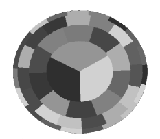
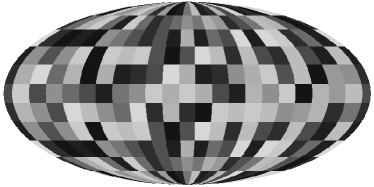
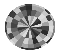
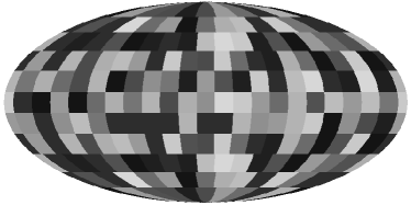
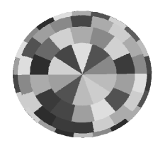
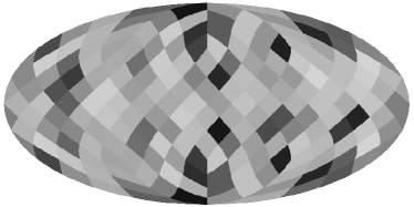
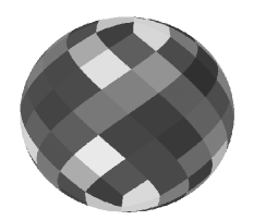
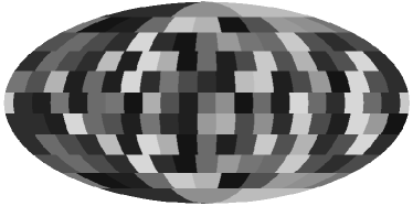
In fig.1, we show the differences in pixelization of the GLESP 1.0, the GLESP-pol (grN), the GLESP-pol (grS) and the HEALPix. One can see, in the central part of the map the properties of the GLESP-pol (grN,grS) are the same as for the GLESP 1.0, but in the vicinity of the polar cups they are significantly different due to over-pixelization. This modification is vital for estimation of the a,m0,±2subscriptsubscript𝑎𝑚0plus-or-minus2{}_{0,\pm 2}a_{\ell,m}-coefficients due to specific behaviour of Y,m±2(θ,ϕ)subscriptsubscript𝑌𝑚plus-or-minus2𝜃italic-ϕ{}_{\pm 2}Y_{\ell,m}(\theta,\phi)-spherical harmonics (see Appendix for details).
Refer to captionRefer to caption

Figure 1: Left column is the Molldweide projection of pixelization grids (from top to bottom): (a) the standard pixelization grid of the GLESP 1.0 (b) the GLESP-pol rectangular grid with the same number of pixels per each ring (the so called case ‘grN’), (c) the GLESP-pol grid with an pixel number increment 4 (case ‘grS’) starting from 10 pixels near poles but not greater than a given resolution in the equator ring, (d) the HEALPix grid. The right column shows the corresponding pixelization in the vicinity of the polar cups.

3 Errors “a,msubscript𝑎𝑚absenta_{\ell,m}\rightarrow mapa,mabsentsubscript𝑎𝑚\rightarrow a_{\ell,m}” transition

This section is devoted to estimation of the error of the a,msubscript𝑎𝑚a_{\ell,m} reconstruction by implementation different regimes of the HEALPix 2.11 and the GLESP-pol (grN and grS) packages. The error bars were defined in the following way. Let us take the coefficients a,mT,E,Bsubscriptsuperscript𝑎𝑇𝐸𝐵𝑚a^{T,E,B}_{\ell,m} for temperature anisotropy T and E and B modes of polarization for ΛΛ\LambdaCDM concordance model by implementation of the Monte Carlo simulation of the random Gaussian signal111We have used the Gaussian signal for simplicity. However, only for the Gaussian signal the power spectrum C()=(2+1)1m=|a,mT,E,B|2𝐶superscript211superscriptsubscript𝑚superscriptsubscriptsuperscript𝑎𝑇𝐸𝐵𝑚2C(\ell)=(2\ell+1)^{-1}\sum_{m=-\ell}^{\ell}|a^{T,E,B}_{\ell,m}|^{2} is the unique characteristic, which determines all the statistical properties.. For the CBBsubscript𝐶𝐵𝐵C_{BB}–spectrum, we have taken a value equal to 1011superscript101110^{-11} just to escape zero in the test calculations.

Then, by implementation of the HEALPix 2.11 and the GLESP-pol packages we used these a,mT,E,Bsubscriptsuperscript𝑎𝑇𝐸𝐵𝑚a^{T,E,B}_{\ell,m} coefficients to create the map of the signal, keeping for both packages the same number of pixels. Thus, the HEALPix map MHisubscriptsuperscript𝑀𝑖𝐻M^{i}_{H}, and the CLESP-pol map MGpsubscriptsuperscript𝑀𝑝𝐺M^{p}_{G} are defined as

MHi=Ha,mT,E,B,MGp=Ga,mT,E,Bformulae-sequencesubscriptsuperscript𝑀𝑖𝐻Hsubscriptsuperscript𝑎𝑇𝐸𝐵𝑚subscriptsuperscript𝑀𝑝𝐺Gsubscriptsuperscript𝑎𝑇𝐸𝐵𝑚\displaystyle M^{i}_{H}=\textbf{H}a^{T,E,B}_{\ell,m},\hskip 14.22636ptM^{p}_{G}=\textbf{G}a^{T,E,B}_{\ell,m} (7)

where H and G are the HEALPix and the GLESP-pol operators for “a,msubscript𝑎𝑚a_{\ell,m} to map” transition, the index i𝑖i marks the number of iteration (0 as default, or 1-4), the index p=1𝑝1p=1 marks the GLESP-pol grN pixelization, and p=2𝑝2p=2 corresponds to the grS pixelization. Let us define the corresponding transition “map to a,msubscript𝑎𝑚a_{\ell,m}” as H1superscriptH1\textbf{H}^{-1} for the HEALPix and G1superscriptG1\textbf{G}^{-1} for the GLESP-pol:

b,mT,E,B=H1MHi=H1Ha,mT,E,B,subscriptsuperscript𝑏𝑇𝐸𝐵𝑚superscriptH1subscriptsuperscript𝑀𝑖𝐻superscriptH1Hsubscriptsuperscript𝑎𝑇𝐸𝐵𝑚\displaystyle b^{T,E,B}_{\ell,m}=\textbf{H}^{-1}M^{i}_{H}=\textbf{H}^{-1}\textbf{H}a^{T,E,B}_{\ell,m},
c,mT,E,B=G1MGp=G1Ga,mT,E,Bsubscriptsuperscript𝑐𝑇𝐸𝐵𝑚superscriptG1subscriptsuperscript𝑀𝑝𝐺superscriptG1Gsubscriptsuperscript𝑎𝑇𝐸𝐵𝑚\displaystyle c^{T,E,B}_{\ell,m}=\textbf{G}^{-1}M^{p}_{G}=\textbf{G}^{-1}\textbf{G}a^{T,E,B}_{\ell,m} (8)

where b,mT,E,Bsubscriptsuperscript𝑏𝑇𝐸𝐵𝑚b^{T,E,B}_{\ell,m} and c,mT,E,Bsubscriptsuperscript𝑐𝑇𝐸𝐵𝑚c^{T,E,B}_{\ell,m} are now the reconstructed coefficients for the HEALPix and GLESP-pol correspondingly. For idealistic case, when a,msubscript𝑎𝑚absenta_{\ell,m}\rightarrow mapa,mabsentsubscript𝑎𝑚\rightarrow a_{\ell,m}” transition has no error bars, the reconstructed b,mT,E,Bsubscriptsuperscript𝑏𝑇𝐸𝐵𝑚b^{T,E,B}_{\ell,m} and c,mT,E,Bsubscriptsuperscript𝑐𝑇𝐸𝐵𝑚c^{T,E,B}_{\ell,m} have to be identical to the input coefficients a,mT,E,Bsubscriptsuperscript𝑎𝑇𝐸𝐵𝑚a^{T,E,B}_{\ell,m}, and H1H=HH1=IsuperscriptH1HsuperscriptHH1I\textbf{H}^{-1}\textbf{H}=\textbf{H}\textbf{H}^{-1}=\textbf{I}, G1G=GG1=IsuperscriptG1GsuperscriptGG1I\textbf{G}^{-1}\textbf{G}=\textbf{G}\textbf{G}^{-1}=\textbf{I}, where I is just a unit matrix. In reality, neither the HEALPix, nor the GLESP-pol packages have non-zero error of the reconstruction due to window functions of the pixels and computational errors for the spherical harmonics. That means that corresponding absolute errors for the “ a,msubscript𝑎𝑚absenta_{\ell,m}\rightarrow mapa,mabsentsubscript𝑎𝑚\rightarrow a_{\ell,m}” transition can be defined as follows:

RHi,m=e(b,mT,E,B)e(a,mT,E,B),IHi,m=m(b,mT,E,B)m(a,mT,E,B),formulae-sequencesubscriptsubscriptsuperscript𝑅𝑖𝐻𝑚𝑒subscriptsuperscript𝑏𝑇𝐸𝐵𝑚𝑒subscriptsuperscript𝑎𝑇𝐸𝐵𝑚subscriptsubscriptsuperscript𝐼𝑖𝐻𝑚𝑚subscriptsuperscript𝑏𝑇𝐸𝐵𝑚𝑚subscriptsuperscript𝑎𝑇𝐸𝐵𝑚\displaystyle{R^{i}_{H}}_{\ell,m}=\Re e(b^{T,E,B}_{\ell,m})-\Re e(a^{T,E,B}_{\ell,m}),\hskip 14.22636pt{I^{i}_{H}}_{\ell,m}=\Im m(b^{T,E,B}_{\ell,m})-\Im m(a^{T,E,B}_{\ell,m}),
RGp,m=e(c,mT,E,B)e(a,mT,E,B),IGp,m=m(c,mT,E,B)m(a,mT,E,B),formulae-sequencesubscriptsubscriptsuperscript𝑅𝑝𝐺𝑚𝑒subscriptsuperscript𝑐𝑇𝐸𝐵𝑚𝑒subscriptsuperscript𝑎𝑇𝐸𝐵𝑚subscriptsubscriptsuperscript𝐼𝑝𝐺𝑚𝑚subscriptsuperscript𝑐𝑇𝐸𝐵𝑚𝑚subscriptsuperscript𝑎𝑇𝐸𝐵𝑚\displaystyle{R^{p}_{G}}_{\ell,m}=\Re e(c^{T,E,B}_{\ell,m})-\Re e(a^{T,E,B}_{\ell,m}),\hskip 14.22636pt{I^{p}_{G}}_{\ell,m}=\Im m(c^{T,E,B}_{\ell,m})-\Im m(a^{T,E,B}_{\ell,m}),
(9)

where e𝑒\Re e and m𝑚\Im m stand for the real and imaginary parts of the coefficients. Thus, the relative error is given by

rHi,m=RHi,me(a,mT,E,B),yHi,m=IHi,mm(a,mT,E,B),formulae-sequencesubscriptsubscriptsuperscript𝑟𝑖𝐻𝑚subscriptsubscriptsuperscript𝑅𝑖𝐻𝑚𝑒subscriptsuperscript𝑎𝑇𝐸𝐵𝑚subscriptsubscriptsuperscript𝑦𝑖𝐻𝑚subscriptsubscriptsuperscript𝐼𝑖𝐻𝑚𝑚subscriptsuperscript𝑎𝑇𝐸𝐵𝑚\displaystyle{r^{i}_{H}}_{\ell,m}=\frac{{R^{i}_{H}}_{\ell,m}}{\Re e(a^{T,E,B}_{\ell,m})},\hskip 14.22636pt{y^{i}_{H}}_{\ell,m}=\frac{{I^{i}_{H}}_{\ell,m}}{\Im m(a^{T,E,B}_{\ell,m})},
rGp,m=RGp,me(a,mT,E,B),yGp,m=IGp,mm(a,mT,E,B),formulae-sequencesubscriptsubscriptsuperscript𝑟𝑝𝐺𝑚subscriptsubscriptsuperscript𝑅𝑝𝐺𝑚𝑒subscriptsuperscript𝑎𝑇𝐸𝐵𝑚subscriptsubscriptsuperscript𝑦𝑝𝐺𝑚subscriptsubscriptsuperscript𝐼𝑝𝐺𝑚𝑚subscriptsuperscript𝑎𝑇𝐸𝐵𝑚\displaystyle{r^{p}_{G}}_{\ell,m}=\frac{{R^{p}_{G}}_{\ell,m}}{\Re e(a^{T,E,B}_{\ell,m})},\hskip 14.22636pt{y^{p}_{G}}_{\ell,m}=\frac{{I^{p}_{G}}_{\ell,m}}{\Im m(a^{T,E,B}_{\ell,m})},
(10)

Note that defined in Eq(10) relative errors are related to the error of the power spectrum

ΔCC=m(|g,m|2|a,m|2)m|a,m|2=m|a,m|2(δ,m+δ,m)m|a,m|2Δsubscript𝐶subscript𝐶subscript𝑚superscriptsubscript𝑔𝑚2superscriptsubscript𝑎𝑚2subscript𝑚superscriptsubscript𝑎𝑚2subscript𝑚superscriptsubscript𝑎𝑚2subscript𝛿𝑚subscriptsuperscript𝛿𝑚subscript𝑚superscriptsubscript𝑎𝑚2\displaystyle\frac{\Delta C_{\ell}}{C_{\ell}}=\frac{\sum_{m}(|g_{\ell,m}|^{2}-|a_{\ell,m}|^{2})}{\sum_{m}|a_{\ell,m}|^{2}}=\frac{\sum_{m}|a_{\ell,m}|^{2}(\delta_{\ell,m}+\delta^{*}_{\ell,m})}{\sum_{m}|a_{\ell,m}|^{2}} (11)

where g,msubscript𝑔𝑚g_{\ell,m} and a,msubscript𝑎𝑚a_{\ell,m} denote the reconstructed and input multipole coefficients, and g,m=a,m(1+δ,m)subscript𝑔𝑚subscript𝑎𝑚1subscript𝛿𝑚g_{\ell,m}=a_{\ell,m}(1+\delta_{\ell,m}). Taking into account that δ,m+δ,m=2e(δ,m)subscript𝛿𝑚subscriptsuperscript𝛿𝑚2𝑒subscript𝛿𝑚\delta_{\ell,m}+\delta^{*}_{\ell,m}=2\Re e(\delta_{\ell,m}) and e(δ,m)=[(ea,m)2r,m+(ma,m)2y,m]/|a,m|2𝑒subscript𝛿𝑚delimited-[]superscript𝑒subscript𝑎𝑚2subscript𝑟𝑚superscript𝑚subscript𝑎𝑚2subscript𝑦𝑚superscriptsubscript𝑎𝑚2\Re e(\delta_{\ell,m})=[(\Re ea_{\ell,m})^{2}r_{\ell,m}+(\Im ma_{\ell,m})^{2}y_{\ell,m}]/|a_{\ell,m}|^{2}, where r,msubscript𝑟𝑚r_{\ell,m} and y,msubscript𝑦𝑚y_{\ell,m} denote relative errors for real and imaginary parts from Eq(10), we gets:

ΔCC=2m[(ea,m)2r,m+(ma,m)2y,m]m|a,m|2Δsubscript𝐶subscript𝐶2subscript𝑚delimited-[]superscript𝑒subscript𝑎𝑚2subscript𝑟𝑚superscript𝑚subscript𝑎𝑚2subscript𝑦𝑚subscript𝑚superscriptsubscript𝑎𝑚2\displaystyle\frac{\Delta C_{\ell}}{C_{\ell}}=2\frac{\sum_{m}[(\Re ea_{\ell,m})^{2}r_{\ell,m}+(\Im ma_{\ell,m})^{2}y_{\ell,m}]}{\sum_{m}|a_{\ell,m}|^{2}} (12)

From Eq(12) clearly seen that the error of reconstruction of real and imaginary part of each ,m𝑚\ell,m coefficient propagates to the error of the power spectrum through weighting coefficients

w,mr=(ea,m)2m|a,m|2,w,my=(ma,m)2m|a,m|2formulae-sequencesubscriptsuperscript𝑤𝑟𝑚superscript𝑒subscript𝑎𝑚2subscript𝑚superscriptsubscript𝑎𝑚2subscriptsuperscript𝑤𝑦𝑚superscript𝑚subscript𝑎𝑚2subscript𝑚superscriptsubscript𝑎𝑚2\displaystyle w^{r}_{\ell,m}=\frac{(\Re ea_{\ell,m})^{2}}{\sum_{m}|a_{\ell,m}|^{2}},\hskip 14.22636ptw^{y}_{\ell,m}=\frac{(\Im ma_{\ell,m})^{2}}{\sum_{m}|a_{\ell,m}|^{2}} (13)

and formally depends on the power spectrum and the morphology of the input signal. This is why in addition to the input random Gaussian CMB signal we will discuss the errors of reconstruction of the multipoles and the power spectrum for very asymmetric maps, like WMAP 5 Q and V bands.

3.1 Errors for HEALPix and GLESP-pol temperature anisotropy

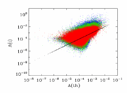
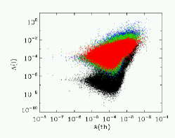
We will start our analysis from estimation of the dynamical range of variations of the temperature anisotropy for Nside=1024. For that we will use the input signal, which corresponds to random Gaussian CMB, and Internal Linear Combination Map (WILC5) from the LAMBDA archive (http://lambda.gsfc.nasa.gov/) and corresponding K, Ka, Q, V and W total channels maps. In Fig2 we plot the diagram A(i)𝐴𝑖A(i) versus A(th)𝐴𝑡A(th), whereA(i)=string(|a,m)|A(i)=string(|a_{\ell,m})|, where the operator ”string” transforms the |a,m|subscript𝑎𝑚|a_{\ell,m}| coefficients to one dimensional string |a1,0|,|a1,1|subscript𝑎10subscript𝑎11|a_{1,0}|,|a_{1,1}|... for K–W bands, and A(th)𝐴𝑡A(th) is the string for the random Gaussian CMB signal.
Refer to captionRefer to captionRefer to caption

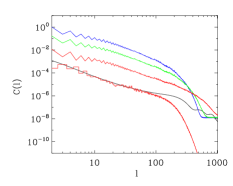
Figure 2: Left. The A(i)𝐴𝑖A(i) versus A(th)𝐴𝑡A(th) diagram for the WILC5 (the black dots), K-band (the blue dots), KA-band (the green dots), V-band (the red dots). Both A(i)𝐴𝑖A(i) and A(th)𝐴𝑡A(th) are in mK. Middle. The same as the left plot, but for replacement of the WILC5 by A(th)𝐴𝑡A(th). Right. The power spectrum C()mK2𝐶𝑚superscript𝐾2C(\ell)mK^{2} for the WILC5 (the red bottom line), for random realization (the black line), the K band ( the solid blue line), the KA-band (the green solid line), and for V band (the red solid line).

From this diagram one can see that, for example, to estimate the a,msubscript𝑎𝑚a_{\ell,m} coefficients by using ILC method we should have, at least, the relative error better than 103104superscript103superscript10410^{-3}-10^{-4} if the low frequency K-band is included to the analysis. T he accuracy of the a,msubscript𝑎𝑚a_{\ell,m} coefficients should be about 3–4 orders of magnitude better if we are interested in different sort of coupling between different multipoles (so called the non-Gaussianity tool).

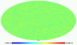
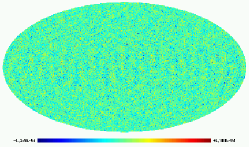
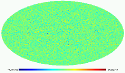
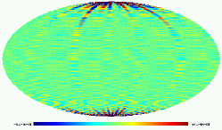
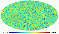
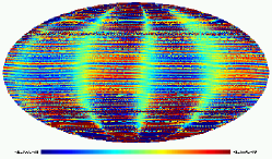
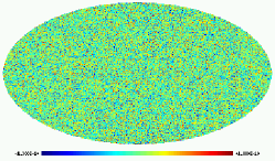
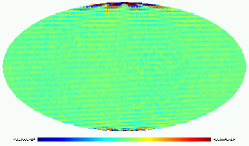
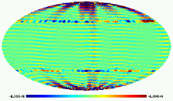
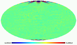
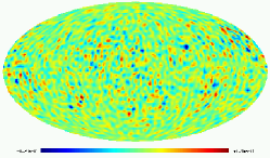
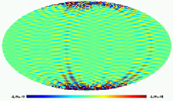
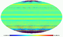
To estimate the errors of the a,msubscript𝑎𝑚absenta_{\ell,m}\rightarrow mapa,mabsentsubscript𝑎𝑚\rightarrow a_{\ell,m}” transition, let us start from the analysis of the temperature anisotropy for the HEALPix 2.11 and the GLESP-pol packages. In Fig.3, we show the maps for b,m0a,msubscriptsuperscript𝑏0𝑚subscript𝑎𝑚b^{0}_{\ell,m}-a_{\ell,m}-signal, where b,m0subscriptsuperscript𝑏0𝑚b^{0}_{\ell,m} obtained by implementation of the HEALPix 2.11 “zero iteration“ key (top left map) and 4 iterations (top right map).
Refer to captionRefer to caption

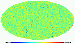
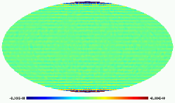
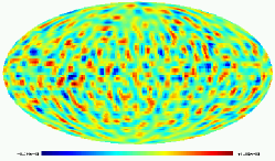
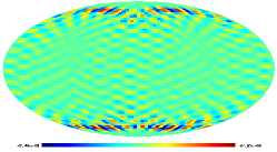
Figure 3: The differences of reconstructed and input maps for the HEALPix 2.11 (the top pair) and the GLESP-pol (the bottom pair). Top left plot corresponds to “zero iteration“ key (the color scale is 106,106mKsuperscript106superscript106𝑚𝐾-10^{-6},10^{-6}mK), top right is for 4 iterations (the color scale is 108,108mKsuperscript108superscript108𝑚𝐾-10^{-8},10^{-8}mK). Bottom left-the GLESP-pol reconstruction for the grN mode (the color scale is 108,108mKsuperscript108superscript108𝑚𝐾-10^{-8},10^{-8}mK). Top right corresponds to the grS mode (the color scale is 108,108mKsuperscript108superscript108𝑚𝐾-10^{-8},10^{-8}mK). The number of pixels for the HEALPix 2.11 and the GLESP-pol are practically the same. No correction by the window function of the pixels.

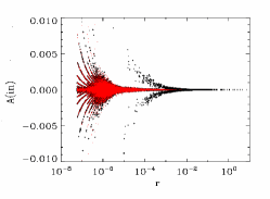
One can see, that the top left map reveals all the peculiarities of the pixelization, localized at the vicinity of the North and the South poles. The top left plot show the map of differences, but after 4 iterations. No visible large scale defects can be found. The bottom left and right maps represent the GLESP-pol pixelization without any iterations for the same number of pixels, as the top one. In Fig.4, we plot the real and imaginary parts of the absolute errors from Eq(9) for the maps, shown in fig.3).
Refer to captionRefer to caption

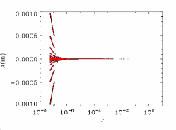
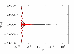
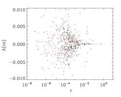
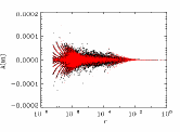
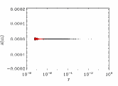
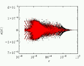
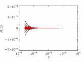
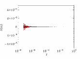
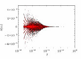
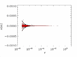
Figure 4: The errors of reconstructions for the HEALPix 2.11 (the top pair) and the GLESP-pol (the bottom pair). Top left plot corresponds to “zero iteration” key, top right is for 4 iterations. Bottom left — the GLESP-pol reconstruction for the grN mode. Top right corresponds to the grS mode. Black dots corresponds to the real part of ,m𝑚\ell,m modes, the red dots show for the imaginary part.

The definition of function A(in)𝐴𝑖𝑛A(in) and r𝑟r in Fig.4 is the following: A(in)=string(a,m)𝐴𝑖𝑛𝑠𝑡𝑟𝑖𝑛𝑔subscript𝑎𝑚A(in)=string(a_{\ell,m}), where the operator ”string” transforms the a,msubscript𝑎𝑚a_{\ell,m} coefficients to one dimensional string a1,0,a1,1subscript𝑎10subscript𝑎11a_{1,0},a_{1,1}..., and r=|rH0,m,rH4,m,yH0,m,yH4,m|r=|{r^{0}_{H}}_{\ell,m},{r^{4}_{H}}_{\ell,m},{y^{0}_{H}}_{\ell,m},{y^{4}_{H}}_{\ell,m}| (see Eq.(10).

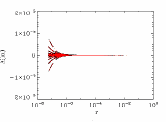
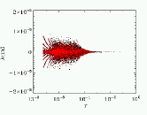
Fig.4 clearly show that the HEALPix 2.11 (no iteration) reconstruction is different for the real and imaginary parts of the signal. For real part (see Fig.4, top left), the relative error has the secondary zone, localized at r>105𝑟superscript105r>10^{-5}, while for imaginary part the major part of the points belongs to r<105𝑟superscript105r<10^{-5}. Note that even after implementation of 4 iterations for the HEALPix 2.11 and grN, grS modes of the GLESP-pol, there exists a very small number (10similar-toabsent10\sim 10) of modes with error 1%-10%. Thus, the main conclusion is that for Nside=1024 the HEALPix iterations significantly improve the global morphology of the map and the error of reconstruction, which is practically the same the HEALPix and the GLESP-pol.

The next question, which we would like to discuss, is how the error of reconstruction depends on the number of pixels and their size. Both these parameters are determined by the choice of Nside for the HEALPix, or by the maximal resolution of the map maxsubscript𝑚𝑎𝑥\ell_{max} for the GLESP-pol. Answering this question in Fig.5 and Fig.6, we plot the corresponding maps of errors and A(in)𝐴𝑖𝑛A(in) versus r𝑟r diagrams, similar to Fig.3 and Fig.4, but for less number of pixels.
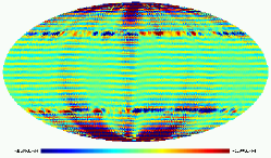
Refer to captionRefer to caption

Figure 5: The differences of reconstructed and input maps for the HEALPix 2.11 for Nside=32 (the top pair) and the GLESP-pol (the bottom pair). Top left plot corresponds to “zero iteration” key (the color scale is 104,104mKsuperscript104superscript104𝑚𝐾-10^{-4},10^{-4}mK), top right is for 4 iterations (the color scale is 8108,8108mK8superscript1088superscript108𝑚𝐾-8\cdot 10^{-8},8\cdot 10^{-8}mK). Bottom left — the GLESP-pol reconstruction for the grN mode (the color scale is 108,108mKsuperscript108superscript108𝑚𝐾-10^{-8},10^{-8}mK). Bottom right corresponds to the grS mode (the color scale is 2.5108,2.5108mK2.5superscript1082.5superscript108𝑚𝐾-2.5\cdot 10^{-8},2.5\cdot 10^{-8}mK). The number of pixels for the HEALPix 2.11 and the GLESP-pol are practically the same. No correction by the window function of the pixels.

Refer to captionRefer to caption

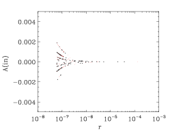
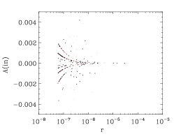
Figure 6: The errors of reconstructions for the HEALPix 2.11 (Nside=32) (the top pair) and the GLESP-pol (the bottom pair). Top left plot corresponds to “zero iteration” key, top right is for 4 iterations. Bottom left — the GLESP-pol reconstruction for the grN mode. Top right corresponds to the grS mode. Black dots corresponds to the real part of ,m𝑚\ell,m modes, the red dots are for imaginary part.

It would be important to note that as for the high resolution map of difference, shown in Fig.3, as for the low resolution map (see Fig.5) for the HEALPix 2.11 with zero iteration the major component of the error is related to b,m=0subscript𝑏𝑚0b_{\ell,m=0} mode. These harmonics manifest themselves as horizontal lines parallel to the Galactic plane. Two horizontal lines with high amplitude signal along mark the HEALPix zones, where the number of pixels for each equal latitude ring start to decrease, when θ0𝜃0\theta\rightarrow 0 (the North pole), or θπ𝜃𝜋\theta\rightarrow\pi (the South pole). However, after 4 iterations all these peculiarities of the map of errors were significantly suppressed, except two zones around the North and the South cups. For the GLESP-pol package with max=32subscript𝑚𝑎𝑥32\ell_{max}=32 the minimal level of errors for the reconstructed map is given by the grN pixelization, when r107much-less-than𝑟superscript107r\ll 10^{-7} for major part of the pixels, and r105much-less-than𝑟superscript105r\ll 10^{-5} for the grS pixelization. It would be important to note that the accuracy of reconstruction of real and imaginary parts of the coefficients of expansion are different for the HEALPix and the GLESP-pol. As it is follows from Fig4 and Fig6, the HEALPix recovers the imaginary part significantly better than a real one even for zero iteration mode. The GLESP-pol reconstructs real and imaginary parts with nearly equal errors.

4 The GLESP-pol and the HEALPix polarization.

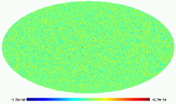
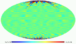
As we have mentioned already in Introduction, the GLESP-pol pixelization was designed to assess the problem of accurate reconstruction of the coefficients of spin ±2plus-or-minus2\pm 2 spherical harmonics decomposition (see Appendix for details). Since the spin ±2plus-or-minus2\pm 2 spherical harmonics have a peculiarity, from the computational point of view, behaviour in the vicinity of the polar cups, the differences in the GLESP-pol polarization and the HEALPix produce different error of reconstruction and become more visible especially for polarization. In Fig.7, we plot the map of differences between input and output signal, reconstructed by the GLESP-pol (grN and grS pixelization).
Refer to captionRefer to caption

Figure 7: The differences of reconstructed and input maps for the GLESP-pol for max=1500subscript𝑚𝑎𝑥1500\ell_{max}=1500 (the top pair is for Q the Stokes parameter) and the bottom pair is for U). Top left plot corresponds to the grN pixelization (the color scale is 31010,31010mK3superscript10103superscript1010𝑚𝐾-3\cdot 10^{-10},3\cdot 10^{-10}mK), top right is for the grS pixelization ( the color scale is 109,109mKsuperscript109superscript109𝑚𝐾-10^{-9},10^{-9}mK). Bottom left — the GLESP-pol reconstruction of Q for grN mode (the color scale is 2.51010,2.51010mK2.5superscript10102.5superscript1010𝑚𝐾-2.5\cdot 10^{-10},2.5\cdot 10^{-10}mK). Bottom right corresponds to the grS mode (the color scale is 109,109mKsuperscript109superscript109𝑚𝐾-10^{-9},10^{-9}mK).

As one can see from this figure, the reconstruction of Q and U components by the grN and grS pixelization is characterized by very high accuracy, but the grN pixelization looks slightly better. For the HEALPix 2.11 the corresponding maps for differences are shown in Fig.8.
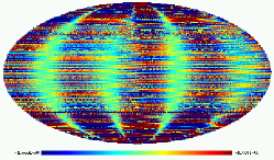
Refer to captionRefer to caption

Figure 8: The differences of reconstructed and input maps for the HEALPix 2.11 for Nside=1024 (the top pair corresponds to Q components and the bottom pair is for U. Top left plot corresponds to the “zero iteration” key (the color scale is 108,108mKsuperscript108superscript108𝑚𝐾-10^{-8},10^{-8}mK), top right is for 4 iterations (the color scale is 1010,1010mKsuperscript1010superscript1010𝑚𝐾10^{-10},10^{-10}mK). Bottom left — the GLESP-pol reconstruction for the grN mode (the color scale is 108,108mKsuperscript108superscript108𝑚𝐾10^{-8},10^{-8}mK). Bottom right corresponds to the grS mode (the color scale is 1010,1010mKsuperscript1010superscript1010𝑚𝐾-10^{-10},10^{-10}mK). The number of pixels for the HEALPix 2.11 and the GLESP-pol are practically the same. No correction by the window function of the pixels.

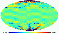
For low resolution pixelization with Nside=32 and max=32subscript𝑚𝑎𝑥32\ell_{max}=32 the corresponding maps are shown in Fig.9
Refer to captionRefer to caption

Figure 9: The differences of reconstructed and input maps for the HEALPix 2.11 for Nside=32 (the top pair corresponds to Q components and the bottom pair is for U. Top left plot corresponds to the “zero iteration” key (the color scale is 106,106mKsuperscript106superscript106𝑚𝐾-10^{-6},10^{-6}mK), top right is for 4 iterations (the color scale is 31010,31010mK3superscript10103superscript1010𝑚𝐾-3\cdot 10^{-10},3\cdot 10^{-10}mK). Bottom left — the U component for the zero iteration (the color scale is 106,106mKsuperscript106superscript106𝑚𝐾-10^{-6},10^{-6}mK). Bottom right corresponds to 4 iterations (the color scale is 31010,31010mK3superscript10103superscript1010𝑚𝐾-3\cdot 10^{-10},3\cdot 10^{-10}mK).

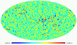
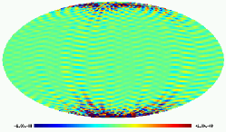
Thus, one can see that implementation of the 4 iterations for the HEALPix package gives us practically the same result, as from GLESP-pol even for the low resolution maps (see Fig.10). In Fig.11 we show the diagram, similar to the Fig.4, but for E and B components of polarization.
Refer to captionRefer to caption

Figure 10: The errors of reconstructions for the GLESP-pol (Q for the top pair and U for the bottom pair). Top left plot corresponds to the grN pixelization (the color scale is 21011,21011mK2superscript10112superscript1011𝑚𝐾-2\cdot 10^{-11},2\cdot 10^{-11}mK), top right is for grN (the color scale is 108,108mKsuperscript108superscript108𝑚𝐾-10^{-8},10^{-8}mK). Bottom left — the GLESP-pol reconstruction for the grS mode (the color scale is 21011,21011mK2superscript10112superscript1011𝑚𝐾-2\cdot 10^{-11},2\cdot 10^{-11}mK. Bottom right corresponds to the grS mode (the color scale is 108,108mKsuperscript108superscript108𝑚𝐾-10^{-8},10^{-8}mK).

Refer to captionRefer to caption Refer to captionRefer to caption

Figure 11: The errors of reconstructions of ea,mE𝑒subscriptsuperscript𝑎𝐸𝑚\Re ea^{E}_{\ell,m} and ma,mE𝑚subscriptsuperscript𝑎𝐸𝑚\Im ma^{E}_{\ell,m}. Top row corresponds to the HEALPix 2.11 (Nside=1024). From the left to the right are: E mode with zero iteration, E mode with 4 iteration, B mode with zero iteration, B mode with 4 iteration. Bottom row is the same, but for the GLESP-pol grN and grS modes and max=1500subscript𝑚𝑎𝑥1500\ell_{max}=1500. Black dots corresponds to the real part of ,m𝑚\ell,m modes, the red dots are for imaginary part.

One can see that the GLESP-pol mode grN gives us practically the same errors, as the HEALPix 2.11 4 iteration mode. However, the CPU time for the GLESP-pol is about 4 time smaller then for the HEALPix 2.11 due to absence of iterations.

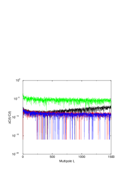
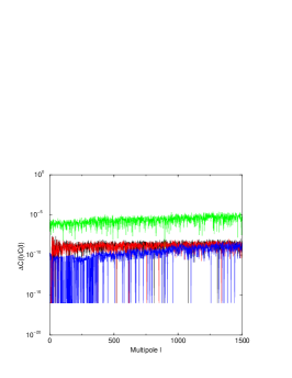
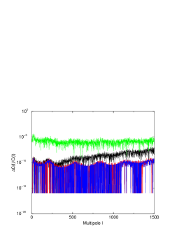
Finally, we demonstrate absolute relative accuracy for power spectra (ΔC()/C()Δ𝐶𝐶\Delta C(\ell)/C(\ell)) for the GLESP 2.0 (grS and grN) and for the HEALPix 2.11 (0 and 4 iteration modes) shown in Fig. (12). As one could see the realtive accuracy for restoration of the power spectrum of temperature anisotropy in the GLESP is approximately the same for both types grS and grN, and the HEALPix 4 iteration mode give better accuracy at low multipoles and reaches the GLESP one at higher. For polarization, we have approximately the same accuracy for the GLESP grN and HEALPix 4 iteration modes.
Refer to caption Refer to caption Refer to caption

Figure 12: The relative accuracy of C()𝐶C(\ell) specrum restoration for temperature anisotropy (left), E-polarization (middle) and B-polarization(right). The grS GLESP type is shown with the black line, the grN type is shown with red, the HEALpix calculations of C()𝐶C(\ell) of 0 iteration mode are plotted with green color, and of 4 iteration with blue.

5 Conclusions

Here we present the GLESP-pol package which incorporates calculations of polarization on the sphere into the CMB analysis package based on the Gauss–Legendre Sky Pixelization. We developed corresponding software for data processing.

According to our numerical calculations, the described scheme for polarization preserves the same level of precision as GLESP 1.0 can provide for the temperature anisotropy.

The code continues to be developed now and different definitions of polarization modes Refs. \refcitekami, \refcitehpix are planned to be included. GLESP-pol is open for new approaches and could be implemented for extension of the present code, e.g. such as the fast spin-weighted harmonics calculation Ref. \refcitewiaux. A completely new algorithm for fast Spherical Harmonics Transform has been proposed recently by Mark Tygert Ref. \refcitetygert. It is worth mentioning that this algorithm can be applied only for GLESP pixelization of the sky and effective as O(A×2Log2)𝑂𝐴superscript2𝐿𝑜subscript𝑔2O(A\times\ell^{2}Log_{2}\ell) operations instead of usual O(3)𝑂superscript3O(\ell^{3}). Unfortunately a huge prefactor A𝐴A makes this algorithm only about 3 times faster than existing HEALPix and GLESP for =20482048\ell=2048.

The most important part of our investigation is that the HEALPix 2.11 package provides the same accuracy as the GLESP-pol only by implementation of 4 iterations. The zero iteration mode of the HEALPix 2.11 can provide significant error for the coefficients of expansion and be used with caution.

Acknowledgments

Athours are very thankful to Radek Stompor for useful remarks to the paper and to Per Rex Christensen for very fruitful discussions and checking GLESP procedures. This paper was supported in part by the RFBR grants 07-02-00886, 08-02-00090, 08-02-00159, 09-02-00298, by S.S. 2469.2008.2 and by FNU grants 272-06-0417, 272-07-0528 and 21-04-0355.

References

  • [1] Hinshaw, G. et al., ApJS170, 288 (2007)
  • [2] Hinshaw, G. et al., ApJS180, 225 (2009)
  • [3] Spergel, G. et al., ApJS170, 377 (2007)
  • [4] Nolta, M.R. et al., ApJS180, 296 (2009)
  • [5] Reichardt, C. L. et al., arXiv:0801.1491 (2008)
  • [6] Pryke, C. et al., ApJ692, 1247 (2009)
  • [7] Hinderks, J. R. et al., ApJ692, 1247 (2009)
  • [8] Challinor A., Lewis A. Phys.Rev. D 71, 103010 (2005)
  • [9] Lewis A., Bridle S. Phys.Rev.D 66, 103511, (2002)
  • [10] Fendt, W. A., Chluba, J., Rubino-Martin, J. A., Wandelt, B. D. arXiv:0807.2577 (2008)
  • [11] Baumann, D. et al., arXiv:0811.3919 (2008)
  • [12] de Bernardis P. et al., arXiv:0808.1881 (2008)
  • [13] Górski, K.M., Hivon, E., Banday, A. J., et al., ApJ622, 759 (2005)
  • [14] Doroshkevich A.G., Naselsky P.D., Verkhodanov O.V., et al. Internat. J. Modern Physics D 14, 275 (2005), astro-ph/0305537
  • [15] Muciaccia P. F., Natoli P. and Vittorio N., Astrophys.J. 488, 63 (1997)
  • [16] Eriksen, H. K. et al., ApJ 605, 14 (2004) astro-ph/0307507
  • [17] Jaffe, T. et al., ApJ 629, L1 (2005), astro-ph/0503213
  • [18] Bridges, M., McEwen, J. D., Lasenby, A. N., Hobson, M. P. MNRAS377, 1473 (2007)
  • [19] Cruz M., Martinez-Gonzales E., Vielva P.,Cayon L., MNRAS, 356, 29, 2005, astro-ph/0405341
  • [20] Eriksen, H. K. et al., ApJ 612, 633 (2004), astro-ph/0403098
  • [21] Chiang Lung-Yih, Naselsky P.D., Verkhodanov O.V., Way M.J. ApJ590, L65 (2003), astro-ph/0303643
  • [22] Naselsky P.D., Doroshkevich A.G., Verkhodanov O.V. ApJ599, L53 (2003), astro-ph/0310542
  • [23] Naselsky P.D., Doroshkevich A.G., Verkhodanov O.V. MNRAS349, 695 (2004), astro-ph/0310601
  • [24] Naselsky P.D., Novikov D.I., Novikov I.D., The Physics of the Cosmoc Microwave Background, Cambridge University Press (2006)
  • [25] Doroshkevich A.G., Naselsky P.D., Verkhodanov O.V., et al., astro-ph/0501494, (2005)
  • [26] Press, W.H., Teukolsky, S.A., Vetterling, W.T., & Flannery, B.P., Numerical Recipes in FORTRAN, Second Edition, Cambridge University Press (1992)
  • [27] Kamionkowski, M., Kosowsky, A., Stebbins, A., Ph.Rev. D 55, 7368 (1997)
  • [28] Wiaux, Y., Jacques, L., Vandergheynst, P., ApJ632, 15 (2005), astro-ph/0502486
  • [29] Tygert M., J. Comput. Phys. 227, 4260 (2008)
  • [30] Varshalovich, D.A., Moscalev, A.N., Khersonskii,V.K., ‘Quantum Theory of Angular Momentus’, (Singapore: World Scientific, 1989)
  • [31] Lewis, A., Challinor, A., Turok, N., Phys. Rev. D 65b, 3505 (2002), astro-ph/0106536
  • [32] Zaldarriaga, M. & Harari, D., Phys. Rev. D 52 3276 (1995)
  • [33] Zaldarriaga, M. & Seljak, U., Phys. Rev. D 55 1830 (1997)
  • [34] Seljak, U. & Zaldarriaga, M., Phys. Rev. Lett. 78, 2054 (1997).
  • [35] Frigo, M. & Johnson, S.G., 1997, The Fastest Fourier Transform in the West, Technical Report MIT-LCS-TR-728, 1997, http://www.fftw.org
  • [36] Hanisch R.J., Farris A., Greisen E.W., et al. Astron. Astrophys, 376, 359 (2001)

6 Appendix

6.1 Description of polarization

6.1.1 Basic relations for the flat space

The polarization is characterized by the symmetric traceless matrix 𝐓𝐓\mathbf{T} composed by two Stokes parameters, Q(𝐱)&U(𝐱)𝑄𝐱𝑈𝐱Q({\bf x})\,\&\,U({\bf x}):

𝐓=(QUUQ)𝐓𝑄𝑈𝑈𝑄\displaystyle\mathbf{T}=\left(\begin{array}[]{cc}Q&U\\ U&-Q\end{array}\right) (16)

The functions Q𝑄Q and U𝑈U depend upon the coordinate frame and components of the tensor Tijsuperscriptsubscript𝑇𝑖𝑗T_{i}^{j} obey the corresponding tensor transformation law:

T~ij=OikOjTksuperscriptsubscript~𝑇𝑖𝑗superscriptsubscript𝑂𝑖𝑘superscriptsubscript𝑂𝑗superscriptsubscript𝑇𝑘\displaystyle\tilde{T}_{i}^{j}=O_{i}^{k}O_{\ell}^{j}T_{k}^{\ell} (17)

where the coordinate transformation is given by x~i=Okixksuperscript~𝑥𝑖subscriptsuperscript𝑂𝑖𝑘superscript𝑥𝑘\tilde{x}^{i}=O^{i}_{k}x^{k}. In particular case under rotation of the coordinate system with the rotation angle ϕitalic-ϕ\phi

𝐎=(cosϕsinϕsinϕcosϕ)𝐎italic-ϕitalic-ϕitalic-ϕitalic-ϕ\displaystyle\mathbf{O}=\left(\begin{array}[]{cc}\cos\phi&\sin\phi\\ -\sin\phi&\cos\phi\end{array}\right) (20)

the functions Q𝑄Q and U𝑈U are transformed as:

Q=Qcos2ϕ+Usin2ϕsuperscript𝑄𝑄2italic-ϕ𝑈2italic-ϕ\displaystyle Q^{\prime}=Q\cos 2\phi+U\sin 2\phi
U=Qsin2ϕ+Ucos2ϕsuperscript𝑈𝑄2italic-ϕ𝑈2italic-ϕ\displaystyle U^{\prime}=-Q\sin 2\phi+U\cos 2\phi (21)

The intensity I2=Q2+U2=12TikTkisuperscript𝐼2superscript𝑄2superscript𝑈212superscriptsubscript𝑇𝑖𝑘subscriptsuperscript𝑇𝑖𝑘I^{2}=Q^{2}+U^{2}=\frac{1}{2}T_{i}^{k}T^{i}_{k} does not depend upon the coordinate system.

6.1.2 Basic relations on the sphere

An arbitrary traceless symmetric tensor can be presented in terms of scalar “electrical”, E𝐸E, and pseudo-scalar “magnetic”, B𝐵B, potentials as:

Tij=(E;i;j12gijE;k;k)+12(ϵikB;j;k+ϵjkB;i;k).\displaystyle T_{ij}=\left(E_{;i;j}-{1\over 2}g_{ij}E_{;k}^{;k}\right)+{1\over 2}\left(\epsilon_{ik}B_{;j}^{;k}+\epsilon_{jk}B^{;k}_{;i}\right)\,. (22)

where ϵijsubscriptitalic-ϵ𝑖𝑗\epsilon_{ij} is the completely antisymmetric tensor (ϵ11=ϵ22=0,ϵ12=ϵ21=sinθformulae-sequencesubscriptitalic-ϵ11subscriptitalic-ϵ220subscriptitalic-ϵ12subscriptitalic-ϵ21𝑠𝑖𝑛𝜃\epsilon_{11}=\epsilon_{22}=0,\,\epsilon_{12}=-\epsilon_{21}=-sin\theta) and ’;’ denotes covariant differentiation on the two dimensional sphere with the metric

dl2=dθ2+sin2θdφ2𝑑superscript𝑙2𝑑superscript𝜃2superscript2𝜃𝑑superscript𝜑2dl^{2}=d\theta^{2}+\sin^{2}\theta d\varphi^{2}

Here θ,φ𝜃𝜑\theta,\varphi are the polar and azimuthal angles. In the case we get instead of (16):

T11=T22=QT21=sinθU,T12=U/sinθ,formulae-sequencesubscriptsuperscript𝑇11subscriptsuperscript𝑇22𝑄formulae-sequencesubscriptsuperscript𝑇12𝜃𝑈subscriptsuperscript𝑇21𝑈𝜃T^{1}_{1}=-T^{2}_{2}=Q\quad T^{1}_{2}=\sin\theta U,\quad T^{2}_{1}=U/\sin\theta\,,

and again we have

I2=0.5TikTki=Q2+U2.superscript𝐼20.5superscriptsubscript𝑇𝑖𝑘superscriptsubscript𝑇𝑘𝑖superscript𝑄2superscript𝑈2I^{2}=0.5T_{i}^{k}T_{k}^{i}=Q^{2}+U^{2}\,.

Stokes parameters Q𝑄Q and U𝑈U are linked with the potentials E𝐸E and B𝐵B as follows:

Q=D1ED2B,U=D2E+D1B,formulae-sequence𝑄subscript𝐷1𝐸subscript𝐷2𝐵𝑈subscript𝐷2𝐸subscript𝐷1𝐵\displaystyle Q=D_{1}E-D_{2}B,\quad U=D_{2}E+D_{1}B\,, (23)

and operators D1subscript𝐷1D_{1} and D2subscript𝐷2D_{2} are:

D1=12(2θ2cotθθ1sin2θ2φ2)=12((1x2)2x211x22φ2)subscript𝐷112superscript2superscript𝜃2𝑐𝑜𝑡𝜃𝜃1superscript2𝜃superscript2superscript𝜑2121superscript𝑥2superscript2superscript𝑥211superscript𝑥2superscript2superscript𝜑2\displaystyle D_{1}={1\over 2}\left({\partial^{2}\over\partial\theta^{2}}-cot\theta{\partial\over\partial\theta}-{1\over\sin^{2}\theta}{\partial^{2}\over\partial\varphi^{2}}\right)={1\over 2}\left((1-x^{2}){\partial^{2}\over\partial x^{2}}-{1\over 1-x^{2}}{\partial^{2}\over\partial\varphi^{2}}\right) (24)
D2=(1sinθ2θφcotθsinθφ)=(2xφ+x1x2φ).subscript𝐷21𝜃superscript2𝜃𝜑𝑐𝑜𝑡𝜃𝜃𝜑superscript2𝑥𝜑𝑥1superscript𝑥2𝜑D_{2}=\left({1\over\sin\theta}{\partial^{2}\over\partial\theta\partial\varphi}-{cot\theta\over\sin\theta}{\partial\over\partial\varphi}\right)=-\left({\partial^{2}\over\partial x\partial\varphi}+{x\over 1-x^{2}}{\partial\over\partial\varphi}\right)\,.

where x=cosθ𝑥𝑐𝑜𝑠𝜃x=cos\theta. These operators are identical with expressions (2.22) and (2.23) in Ref. \refcitekami.

6.1.3 Spherical harmonics

Following to Refs. \refciteglesp, reficiteglespa we use the representation of scalar (“electrical”), E𝐸E, and pseudoscalar (“magnetic”), B𝐵B, polarization potentials identical to (1):

E=12π=2max(e0f0(x)+2m=1fm(x)[emccos(mφ)emssin(mφ)]),𝐸12𝜋superscriptsubscript2subscript𝑚𝑎𝑥subscript𝑒0subscriptsuperscript𝑓0𝑥2superscriptsubscript𝑚1subscriptsuperscript𝑓𝑚𝑥delimited-[]superscriptsubscript𝑒𝑚𝑐𝑚𝜑superscriptsubscript𝑒𝑚𝑠𝑚𝜑\displaystyle E={1\over\sqrt{2\pi}}\sum_{\ell=2}^{\ell_{max}}\left(e_{\ell 0}f^{0}_{\ell}(x)+2\sum_{m=1}^{\ell}f^{m}_{\ell}(x)[e_{\ell m}^{c}\cos(m\varphi)-e_{\ell m}^{s}\sin(m\varphi)]\right)\,, (25)
B=12π=2max(b0f0(x)+2m=1fm(x)[bmccos(mφ)bmssin(mφ)]),𝐵12𝜋superscriptsubscript2subscript𝑚𝑎𝑥subscript𝑏0subscriptsuperscript𝑓0𝑥2superscriptsubscript𝑚1subscriptsuperscript𝑓𝑚𝑥delimited-[]superscriptsubscript𝑏𝑚𝑐𝑚𝜑superscriptsubscript𝑏𝑚𝑠𝑚𝜑\displaystyle B={1\over\sqrt{2\pi}}\sum_{\ell=2}^{\ell_{max}}\left(b_{\ell 0}f^{0}_{\ell}(x)+2\sum_{m=1}^{\ell}f^{m}_{\ell}(x)[b_{\ell m}^{c}\cos(m\varphi)-b_{\ell m}^{s}\sin(m\varphi)]\right)\,, (26)
fm=(+0.5)(m)!(+m)!Bm,0mlmax,formulae-sequencesuperscriptsubscript𝑓𝑚0.5𝑚𝑚superscriptsubscript𝐵𝑚0𝑚subscript𝑙𝑚𝑎𝑥\displaystyle f_{\ell}^{m}=\sqrt{(\ell+0.5){(\ell-m)!\over(\ell+m)!}}B_{\ell}^{m},\quad 0\leq m\leq\ell\leq l_{max}\,, (27)

Here Bm(x)superscriptsubscript𝐵𝑚𝑥B_{\ell}^{m}(x) and fm(x)superscriptsubscript𝑓𝑚𝑥f_{\ell}^{m}(x) are the associated Legendre functions (ordinary and normalized) and emsubscript𝑒𝑚e_{\ell m} and bmsubscript𝑏𝑚b_{\ell m} are the coefficients of decomposition characterizing properties of polarization.

emc=12π11𝑑x02π𝑑φE(x,φ)fm(x)cosmφ,superscriptsubscript𝑒𝑚𝑐12𝜋superscriptsubscript11differential-d𝑥superscriptsubscript02𝜋differential-d𝜑𝐸𝑥𝜑superscriptsubscript𝑓𝑚𝑥𝑚𝜑\displaystyle e_{\ell m}^{c}={1\over\sqrt{2\pi}}\int_{-1}^{1}dx\int_{0}^{2\pi}d\varphi E(x,\varphi)f_{\ell}^{m}(x)\cos m\varphi, (28)
ems=12π11𝑑x02π𝑑φE(x,φ)fm(x)sinmφ.superscriptsubscript𝑒𝑚𝑠12𝜋superscriptsubscript11differential-d𝑥superscriptsubscript02𝜋differential-d𝜑𝐸𝑥𝜑superscriptsubscript𝑓𝑚𝑥𝑚𝜑e_{\ell m}^{s}={1\over\sqrt{2\pi}}\int_{-1}^{1}dx\int_{0}^{2\pi}d\varphi E(x,\varphi)f_{\ell}^{m}(x)\sin m\varphi\,.

Similar expressions for the “magnetic” mode can be obtained by replacing of emc&emssuperscriptsubscript𝑒𝑚𝑐superscriptsubscript𝑒𝑚𝑠e_{\ell m}^{c}\,\&\,e_{\ell m}^{s} with bmc&bmssuperscriptsubscript𝑏𝑚𝑐superscriptsubscript𝑏𝑚𝑠b_{\ell m}^{c}\,\&\,b_{\ell m}^{s} and E𝐸E with B𝐵B.

As in the previous package the functions fm(x)superscriptsubscript𝑓𝑚𝑥f_{\ell}^{m}(x) are found recursively:

fm(x)=x4l212m2f1m2+12l3(1)2m22m2f2m,superscriptsubscript𝑓𝑚𝑥𝑥4superscript𝑙21superscript2superscript𝑚2superscriptsubscript𝑓1𝑚212𝑙3superscript12superscript𝑚2superscript2superscript𝑚2superscriptsubscript𝑓2𝑚\displaystyle f_{\ell}^{m}(x)=x\sqrt{4l^{2}-1\over\ell^{2}-m^{2}}f_{\ell-1}^{m}-\sqrt{{2\ell+1\over 2l-3}{(\ell-1)^{2}-m^{2}\over\ell^{2}-m^{2}}}f_{\ell-2}^{m}\,, (29)

or

fm=2(m1)2m2++mxfm11x2+2m+1m+m1+mfm2,superscriptsubscript𝑓𝑚2𝑚1superscript2superscript𝑚2𝑚𝑥superscriptsubscript𝑓𝑚11superscript𝑥22𝑚1𝑚𝑚1𝑚superscriptsubscript𝑓𝑚2\displaystyle f_{\ell}^{m}=-{2(m-1)\over\sqrt{\ell^{2}-m^{2}+\ell+m}}{xf_{\ell}^{m-1}\over\sqrt{1-x^{2}}}-\sqrt{{\ell+2-m\over\ell+1-m}\,{\ell+m-1\over\ell+m}}f_{\ell}^{m-2}, (30)
fmm=(1)m(2m+1)!!2(2m)!!(1x2)m/2,fm+1m=x2m+3fmm.formulae-sequencesuperscriptsubscript𝑓𝑚𝑚superscript1𝑚double-factorial2𝑚12double-factorial2𝑚superscript1superscript𝑥2𝑚2subscriptsuperscript𝑓𝑚𝑚1𝑥2𝑚3subscriptsuperscript𝑓𝑚𝑚\displaystyle f_{m}^{m}=(-1)^{m}\sqrt{(2m+1)!!\over 2(2m)!!}(1-x^{2})^{m/2},\quad f^{m}_{m+1}=x\sqrt{2m+3}f^{m}_{m}\,. (31)

Relation (29) starts with fmmsuperscriptsubscript𝑓𝑚𝑚f_{m}^{m} and fm+1msuperscriptsubscript𝑓𝑚1𝑚f_{m+1}^{m} (31) and generates functions fmsuperscriptsubscript𝑓𝑚f_{\ell}^{m} for all m𝑚\ell\geq m. Relation (30) starts with fmmsuperscriptsubscript𝑓𝑚𝑚f_{m}^{m} and f0superscriptsubscript𝑓0f_{\ell}^{0} and generates functions fmsuperscriptsubscript𝑓𝑚f_{\ell}^{m} for all 1ml1𝑚𝑙1\leq m\leq l. In the case function f0superscriptsubscript𝑓0f_{\ell}^{0} must be found with relation (29).

It is easy to see that

D1E=Fm[emccos(mφ)emssin(mφ)],subscript𝐷1𝐸superscriptsubscript𝐹𝑚delimited-[]superscriptsubscript𝑒𝑚𝑐𝑚𝜑superscriptsubscript𝑒𝑚𝑠𝑚𝜑\displaystyle D_{1}E=F_{\ell}^{m}[e_{\ell m}^{c}\cos(m\varphi)-e_{\ell m}^{s}\sin(m\varphi)]\,, (32)
D2E=Φm[emcsin(mφ)+emscos(mφ)],subscript𝐷2𝐸superscriptsubscriptΦ𝑚delimited-[]superscriptsubscript𝑒𝑚𝑐𝑚𝜑superscriptsubscript𝑒𝑚𝑠𝑚𝜑\displaystyle D_{2}E=\Phi_{\ell}^{m}[e_{\ell m}^{c}\sin(m\varphi)+e_{\ell m}^{s}\cos(m\varphi)]\,, (33)

where functions Fmsuperscriptsubscript𝐹𝑚F_{\ell}^{m} and ΦmsuperscriptsubscriptΦ𝑚\Phi_{\ell}^{m} are expressed through the normalized Legendre functions (29,30):

MFm=2+121(2m2)xf1m1x2+(m2)fm1x2(1)2fm,subscript𝑀superscriptsubscript𝐹𝑚2121superscript2superscript𝑚2𝑥superscriptsubscript𝑓1𝑚1superscript𝑥2superscript𝑚2superscriptsubscript𝑓𝑚1superscript𝑥212superscriptsubscript𝑓𝑚\displaystyle M_{\ell}F_{\ell}^{m}=\sqrt{{2\ell+1\over 2\ell-1}(\ell^{2}-m^{2})}\,\,{xf_{\ell-1}^{m}\over 1-x^{2}}+{(m^{2}-\ell)f_{\ell}^{m}\over 1-x^{2}}-{\ell(\ell-1)\over 2}f_{\ell}^{m}, (34)
MΦm=m1x2[2+121(2m2)f1m(1)xfm],subscript𝑀superscriptsubscriptΦ𝑚𝑚1superscript𝑥2delimited-[]2121superscript2superscript𝑚2superscriptsubscript𝑓1𝑚1𝑥superscriptsubscript𝑓𝑚\displaystyle M_{\ell}\Phi_{\ell}^{m}={m\over 1-x^{2}}\left[\sqrt{{2\ell+1\over 2\ell-1}(\ell^{2}-m^{2})}f_{\ell-1}^{m}-(\ell-1)xf_{\ell}^{m}\right]\,, (35)

or by other way

MFm=m11x2mfm2+2m2fm2m2+m1x2xfm+1,subscript𝑀superscriptsubscript𝐹𝑚𝑚11superscript𝑥2𝑚superscriptsubscript𝑓𝑚superscript22𝑚2subscriptsuperscript𝑓𝑚superscript2superscript𝑚2𝑚1superscript𝑥2𝑥superscriptsubscript𝑓𝑚1\displaystyle M_{\ell}F_{\ell}^{m}={m-1\over 1-x^{2}}mf_{\ell}^{m}-{\ell^{2}+\ell-2m\over 2}f^{m}_{\ell}-\sqrt{\ell^{2}-m^{2}+\ell-m\over 1-x^{2}}{xf_{\ell}^{m+1}}\,,\,\, (36)
MΦm=m[(+m+1)(m)1x2fm+1+(m1)x1x2fm].subscript𝑀superscriptsubscriptΦ𝑚𝑚delimited-[]𝑚1𝑚1superscript𝑥2subscriptsuperscript𝑓𝑚1𝑚1𝑥1superscript𝑥2subscriptsuperscript𝑓𝑚\displaystyle M_{\ell}\Phi_{\ell}^{m}=-m\left[{\sqrt{(\ell+m+1)(\ell-m)}\over\sqrt{1-x^{2}}}f^{m+1}_{\ell}+(m-1){x\over 1-x^{2}}f^{m}_{\ell}\right]\,. (37)

Here

M2=0.25(+2)(+1)(1),superscriptsubscript𝑀20.25211\displaystyle M_{\ell}^{2}=0.25(\ell+2)(\ell+1)\ell(\ell-1), (38)

and functions Fmsuperscriptsubscript𝐹𝑚F_{\ell}^{m} and ΦmsuperscriptsubscriptΦ𝑚\Phi_{\ell}^{m} are normalized by condition

11(Fm+Φm)2𝑑x=11[(Fm)2+(Φm)2]𝑑x=1.superscriptsubscript11superscriptsuperscriptsubscript𝐹𝑚superscriptsubscriptΦ𝑚2differential-d𝑥superscriptsubscript11delimited-[]superscriptsuperscriptsubscript𝐹𝑚2superscriptsuperscriptsubscriptΦ𝑚2differential-d𝑥1\int_{-1}^{1}(F_{\ell}^{m}+\Phi_{\ell}^{m})^{2}dx=\int_{-1}^{1}[(F_{\ell}^{m})^{2}+(\Phi_{\ell}^{m})^{2}]dx=1\,.

In particular,

Fmm=m12Mmm1+x21x2fmm,Fm+1m=mxfmm2m+3Mm+1[m11x2m+12],formulae-sequencesubscriptsuperscript𝐹𝑚𝑚𝑚12subscript𝑀𝑚𝑚1superscript𝑥21superscript𝑥2subscriptsuperscript𝑓𝑚𝑚subscriptsuperscript𝐹𝑚𝑚1𝑚𝑥subscriptsuperscript𝑓𝑚𝑚2𝑚3subscript𝑀𝑚1delimited-[]𝑚11superscript𝑥2𝑚12F^{m}_{m}={m-1\over 2M_{m}}m{1+x^{2}\over 1-x^{2}}f^{m}_{m},\quad F^{m}_{m+1}=mxf^{m}_{m}{\sqrt{2m+3}\over M_{m+1}}\left[{m-1\over 1-x^{2}}-{m+1\over 2}\right],
Φmm=m(m1)Mm(1x2)xfmm,Φm+1m=mfmm2m+3Mm+11mx21x2,formulae-sequencesuperscriptsubscriptΦ𝑚𝑚𝑚𝑚1subscript𝑀𝑚1superscript𝑥2𝑥subscriptsuperscript𝑓𝑚𝑚subscriptsuperscriptΦ𝑚𝑚1𝑚subscriptsuperscript𝑓𝑚𝑚2𝑚3subscript𝑀𝑚11𝑚superscript𝑥21superscript𝑥2\displaystyle\Phi_{m}^{m}=-{m(m-1)\over M_{m}(1-x^{2})}xf^{m}_{m},\quad\Phi^{m}_{m+1}=mf^{m}_{m}{\sqrt{2m+3}\over M_{m+1}}\,\,{1-mx^{2}\over 1-x^{2}}\,, (39)

Combining (23), (24), (25) and (26), we get for functions Q,&U𝑄𝑈Q,\,\&\,U:

Qcm(x)=12π02π𝑑φQcosmφ==2max(Fm(x)emcΦm(x)bms),subscriptsuperscript𝑄𝑚𝑐𝑥12𝜋superscriptsubscript02𝜋differential-d𝜑𝑄𝑚𝜑superscriptsubscript2subscript𝑚𝑎𝑥superscriptsubscript𝐹𝑚𝑥superscriptsubscript𝑒𝑚𝑐superscriptsubscriptΦ𝑚𝑥superscriptsubscript𝑏𝑚𝑠\displaystyle Q^{m}_{c}(x)={1\over\sqrt{2\pi}}\int_{0}^{2\pi}d\varphi Q\cos m\varphi=\sum_{\ell=2}^{\ell_{max}}(F_{\ell}^{m}(x)e_{\ell m}^{c}-\Phi_{\ell}^{m}(x)b_{\ell m}^{s})\,, (40)
Qsm(x)=12π02π𝑑φQsinmφ==2max(Fm(x)emsΦm(x)bmc),subscriptsuperscript𝑄𝑚𝑠𝑥12𝜋superscriptsubscript02𝜋differential-d𝜑𝑄𝑚𝜑superscriptsubscript2subscript𝑚𝑎𝑥superscriptsubscript𝐹𝑚𝑥superscriptsubscript𝑒𝑚𝑠superscriptsubscriptΦ𝑚𝑥superscriptsubscript𝑏𝑚𝑐\displaystyle Q^{m}_{s}(x)={1\over\sqrt{2\pi}}\int_{0}^{2\pi}d\varphi Q\sin m\varphi=\sum_{\ell=2}^{\ell_{max}}(-F_{\ell}^{m}(x)e_{\ell m}^{s}-\Phi_{\ell}^{m}(x)b_{\ell m}^{c})\,, (41)
Ucm(x)=12π02π𝑑φUcosmφ==2max(Φm(x)ems+Fm(x)bmc),subscriptsuperscript𝑈𝑚𝑐𝑥12𝜋superscriptsubscript02𝜋differential-d𝜑𝑈𝑚𝜑superscriptsubscript2subscript𝑚𝑎𝑥superscriptsubscriptΦ𝑚𝑥superscriptsubscript𝑒𝑚𝑠superscriptsubscript𝐹𝑚𝑥superscriptsubscript𝑏𝑚𝑐\displaystyle U^{m}_{c}(x)={1\over\sqrt{2\pi}}\int_{0}^{2\pi}d\varphi U\cos m\varphi=\sum_{\ell=2}^{\ell_{max}}(\Phi_{\ell}^{m}(x)e_{\ell m}^{s}+F_{\ell}^{m}(x)b_{\ell m}^{c})\,, (42)
Usm(x)=12π02π𝑑φUsinmφ==2max(Φm(x)emcFm(x)bms),subscriptsuperscript𝑈𝑚𝑠𝑥12𝜋superscriptsubscript02𝜋differential-d𝜑𝑈𝑚𝜑superscriptsubscript2subscript𝑚𝑎𝑥superscriptsubscriptΦ𝑚𝑥superscriptsubscript𝑒𝑚𝑐superscriptsubscript𝐹𝑚𝑥superscriptsubscript𝑏𝑚𝑠\displaystyle U^{m}_{s}(x)={1\over\sqrt{2\pi}}\int_{0}^{2\pi}d\varphi U\sin m\varphi=\sum_{\ell=2}^{\ell_{max}}(\Phi_{\ell}^{m}(x)e_{\ell m}^{c}-F_{\ell}^{m}(x)b_{\ell m}^{s})\,, (43)

6.1.4 Spin–weight functions

Functions Fmsuperscriptsubscript𝐹𝑚F_{\ell}^{m} and ΦmsuperscriptsubscriptΦ𝑚\Phi_{\ell}^{m} do not form an orthogonal basis and to perform the further decomposition of polarization we need to use the normalized spin - weight spherical functions which can be defined as follows:

λ,m+=Fm+Φm,λ,m=FmΦm,formulae-sequencesuperscriptsubscript𝜆𝑚superscriptsubscript𝐹𝑚superscriptsubscriptΦ𝑚superscriptsubscript𝜆𝑚superscriptsubscript𝐹𝑚superscriptsubscriptΦ𝑚\displaystyle\lambda_{\ell,m}^{+}=F_{\ell}^{m}+\Phi_{\ell}^{m},\quad\lambda_{\ell,m}^{-}=F_{\ell}^{m}-\Phi_{\ell}^{m},\, (44)
λ,m+(x)=(1)m+λ,m(x),λ,m(x)=(1)m+λ,m+(x),formulae-sequencesubscriptsuperscript𝜆𝑚𝑥superscript1𝑚subscriptsuperscript𝜆𝑚𝑥subscriptsuperscript𝜆𝑚𝑥superscript1𝑚subscriptsuperscript𝜆𝑚𝑥\displaystyle\lambda^{+}_{\ell,m}(x)=(-1)^{m+\ell}\lambda^{-}_{\ell,m}(-x),\quad\lambda^{-}_{\ell,m}(x)=(-1)^{m+\ell}\lambda^{+}_{\ell,m}(-x)\,, (45)

These functions satisfy the self-adjoint equation:

ddx[(1x2)ddxλ,m]4+m2+4mx1x2λ,m+(+1)λ,m=0,𝑑𝑑𝑥delimited-[]1superscript𝑥2𝑑𝑑𝑥subscript𝜆𝑚4superscript𝑚24𝑚𝑥1superscript𝑥2subscript𝜆𝑚1subscript𝜆𝑚0{d\over dx}\left[(1-x^{2}){d\over dx}\lambda_{\ell,m}\right]-{4+m^{2}+4mx\over 1-x^{2}}\lambda_{\ell,m}+\ell(\ell+1)\lambda_{\ell,m}=0\,,

and, so, they are orthogonal for a given m𝑚m (see, e.g., \refcitevarsh, \refcitelewis and references there). Some of this functions can be written directly:

λm,m+=Am,m(1)m(1x)2(1x2)m22=Fmm+Φmm,superscriptsubscript𝜆𝑚𝑚subscript𝐴𝑚𝑚superscript1𝑚superscript1𝑥2superscript1superscript𝑥2𝑚22subscriptsuperscript𝐹𝑚𝑚subscriptsuperscriptΦ𝑚𝑚\lambda_{m,m}^{+}=A_{m,m}(-1)^{m}(1-x)^{2}(1-x^{2})^{m-2\over 2}=F^{m}_{m}+\Phi^{m}_{m}\,,
λm+1,m+=Am+1,m(1)m(1x)2(1x2)m22[2+(m+1)x]=Fm+1m+Φm+1m,superscriptsubscript𝜆𝑚1𝑚subscript𝐴𝑚1𝑚superscript1𝑚superscript1𝑥2superscript1superscript𝑥2𝑚22delimited-[]2𝑚1𝑥subscriptsuperscript𝐹𝑚𝑚1subscriptsuperscriptΦ𝑚𝑚1\lambda_{m+1,m}^{+}=A_{m+1,m}(-1)^{m}(1-x)^{2}(1-x^{2})^{m-2\over 2}[2+(m+1)x]=F^{m}_{m+1}+\Phi^{m}_{m+1}\,,
Am,m2=m(m1)(2m+1)!!(m+2)(2m+2)!!,Am+1,m2=2m+3(m+3)(m1)Am,m2.formulae-sequencesuperscriptsubscript𝐴𝑚𝑚2𝑚𝑚1double-factorial2𝑚1𝑚2double-factorial2𝑚2superscriptsubscript𝐴𝑚1𝑚22𝑚3𝑚3𝑚1superscriptsubscript𝐴𝑚𝑚2A_{m,m}^{2}={m(m-1)(2m+1)!!\over(m+2)(2m+2)!!},\quad A_{m+1,m}^{2}={2m+3\over(m+3)(m-1)}A_{m,m}^{2}\,.

and using these relations functions λ,msubscript𝜆𝑚\lambda_{\ell,m} with >m+1𝑚1\ell>m+1 can be evaluated recursively:

λ,m=(x+2m(1))C,mλ1,mC,mC1,mλ2,m,subscript𝜆𝑚𝑥2𝑚1subscript𝐶𝑚subscript𝜆1𝑚subscript𝐶𝑚subscript𝐶1𝑚subscript𝜆2𝑚\displaystyle\lambda_{\ell,m}=\left(x+{2m\over\ell(\ell-1)}\right)C_{\ell,m}\lambda_{\ell-1,m}-{C_{\ell,m}\over C_{\ell-1,m}}\lambda_{\ell-2,m}\,, (46)
C,m=2(421)(2m2)(24).subscript𝐶𝑚superscript24superscript21superscript2superscript𝑚2superscript24C_{\ell,m}=\sqrt{\ell^{2}(4\ell^{2}-1)\over(\ell^{2}-m^{2})(\ell^{2}-4)}\,.
11𝑑x[Fm(x)Fkm(x)+Φm(x)Φkm(x)]=δk,superscriptsubscript11differential-d𝑥delimited-[]subscriptsuperscript𝐹𝑚𝑥superscriptsubscript𝐹𝑘𝑚𝑥subscriptsuperscriptΦ𝑚𝑥superscriptsubscriptΦ𝑘𝑚𝑥subscript𝛿𝑘\int_{-1}^{1}dx[F^{m}_{\ell}(x)F_{k}^{m}(x)+\Phi^{m}_{\ell}(x)\Phi_{k}^{m}(x)]=\delta_{k\ell}\,,
11𝑑x[Fm(x)Φkm(x)+Φm(x)Fkm(x)]=0.superscriptsubscript11differential-d𝑥delimited-[]subscriptsuperscript𝐹𝑚𝑥superscriptsubscriptΦ𝑘𝑚𝑥subscriptsuperscriptΦ𝑚𝑥superscriptsubscript𝐹𝑘𝑚𝑥0\int_{-1}^{1}dx[F^{m}_{\ell}(x)\Phi_{k}^{m}(x)+\Phi^{m}_{\ell}(x)F_{k}^{m}(x)]=0\,.

This means that coefficients for the decomposition of Q𝑄Q and U𝑈U can be found from (40 - 43) as follows:

emc=11𝑑x[Φm(x)Usm(x)+Fm(x)Qcm(x)],superscriptsubscript𝑒𝑚𝑐superscriptsubscript11differential-d𝑥delimited-[]subscriptsuperscriptΦ𝑚𝑥superscriptsubscript𝑈𝑠𝑚𝑥subscriptsuperscript𝐹𝑚𝑥superscriptsubscript𝑄𝑐𝑚𝑥\displaystyle e_{\ell m}^{c}=\int_{-1}^{1}dx[\Phi^{m}_{\ell}(x)U_{s}^{m}(x)+F^{m}_{\ell}(x)Q_{c}^{m}(x)]\,, (47)
ems=11𝑑x[Φm(x)Ucm(x)Fm(x)Qsm(x)],subscriptsuperscript𝑒𝑠𝑚superscriptsubscript11differential-d𝑥delimited-[]subscriptsuperscriptΦ𝑚𝑥superscriptsubscript𝑈𝑐𝑚𝑥subscriptsuperscript𝐹𝑚𝑥superscriptsubscript𝑄𝑠𝑚𝑥\displaystyle e^{s}_{\ell m}=\int_{-1}^{1}dx[\Phi^{m}_{\ell}(x)U_{c}^{m}(x)-F^{m}_{\ell}(x)Q_{s}^{m}(x)]\,, (48)
bmc=11𝑑x[Fm(x)Ucm(x)Φm(x)Qsm(x)],superscriptsubscript𝑏𝑚𝑐superscriptsubscript11differential-d𝑥delimited-[]subscriptsuperscript𝐹𝑚𝑥superscriptsubscript𝑈𝑐𝑚𝑥subscriptsuperscriptΦ𝑚𝑥superscriptsubscript𝑄𝑠𝑚𝑥\displaystyle b_{\ell m}^{c}=\int_{-1}^{1}dx[F^{m}_{\ell}(x)U_{c}^{m}(x)-\Phi^{m}_{\ell}(x)Q_{s}^{m}(x)]\,, (49)
bms=11𝑑x[Fm(x)Usm(x)Φm(x)Qcm(x)],subscriptsuperscript𝑏𝑠𝑚superscriptsubscript11differential-d𝑥delimited-[]subscriptsuperscript𝐹𝑚𝑥superscriptsubscript𝑈𝑠𝑚𝑥subscriptsuperscriptΦ𝑚𝑥superscriptsubscript𝑄𝑐𝑚𝑥\displaystyle b^{s}_{\ell m}=\int_{-1}^{1}dx[-F^{m}_{\ell}(x)U_{s}^{m}(x)-\Phi^{m}_{\ell}(x)Q_{c}^{m}(x)]\,, (50)

For numerical analysis of the polarization maps together with the temperature fluctuations it is convenient to use relations (27 - 37) and (47 - 50) instead of the recursive relations (46). Inverse problem that is the construction of the polarization maps from coefficients em&bmsubscript𝑒𝑚subscript𝑏𝑚e_{\ell m}\,\&\,b_{\ell m} can also be solved using relations (40 - 43).

6.1.5 Spectra of the anisotropy and polarization

Four power spectra can be introduced for the temperature, electrical and magnetic Stokes parameters, they are:

CT=12+1m=|am|2,subscriptsuperscript𝐶𝑇121superscriptsubscript𝑚superscriptsubscript𝑎𝑚2C^{T}_{\ell}={1\over 2\ell+1}\sum_{m=-\ell}^{\ell}|a_{\ell m}|^{2}\,,
CE=12+1m=0[(emc)2+(ems)2],subscriptsuperscript𝐶𝐸121superscriptsubscript𝑚0delimited-[]superscriptsuperscriptsubscript𝑒𝑚𝑐2superscriptsuperscriptsubscript𝑒𝑚𝑠2\displaystyle C^{E}_{\ell}={1\over 2\ell+1}\sum_{m=0}^{\ell}[(e_{\ell m}^{c})^{2}+(e_{\ell m}^{s})^{2}]\,, (51)
CB=12+1m=0[(bmc)2+(bms)2],subscriptsuperscript𝐶𝐵121superscriptsubscript𝑚0delimited-[]superscriptsuperscriptsubscript𝑏𝑚𝑐2superscriptsuperscriptsubscript𝑏𝑚𝑠2C^{B}_{\ell}={1\over 2\ell+1}\sum_{m=0}^{\ell}[(b_{\ell m}^{c})^{2}+(b_{\ell m}^{s})^{2}]\,,
CTE=12+1m=0[amcemc+amsems],subscriptsuperscript𝐶𝑇𝐸121superscriptsubscript𝑚0delimited-[]superscriptsubscript𝑎𝑚𝑐superscriptsubscript𝑒𝑚𝑐superscriptsubscript𝑎𝑚𝑠superscriptsubscript𝑒𝑚𝑠C^{TE}_{\ell}={1\over 2\ell+1}\sum_{m=0}^{\ell}[a_{\ell m}^{c}e_{\ell m}^{c}+a_{\ell m}^{s}e_{\ell m}^{s}]\,,

When averaged over the sky, the mean square temperature anisotropy is

ΔT2=T02=22+14πCT,delimited-⟨⟩Δsuperscript𝑇2superscriptsubscript𝑇02superscriptsubscript2214𝜋subscriptsuperscript𝐶𝑇\displaystyle\langle\Delta T^{2}\rangle=T_{0}^{2}\sum_{\ell=2}^{\infty}{2\ell+1\over 4\pi}C^{T}_{\ell}\,, (52)

where T0subscript𝑇0T_{0} is the temperature of the CMB. The mean square of polarization is

I2=12Q2+U2=12[E2+B2]delimited-⟨⟩superscript𝐼212delimited-⟨⟩superscript𝑄2superscript𝑈212delimited-[]delimited-⟨⟩subscriptsuperscript𝐸2delimited-⟨⟩subscriptsuperscript𝐵2\langle I^{2}\rangle={1\over 2}\langle Q^{2}+U^{2}\rangle={1\over 2}[\langle E^{2}_{*}\rangle+\langle B^{2}_{*}\rangle]

where

E2=T02=22+14πCE,delimited-⟨⟩subscriptsuperscript𝐸2superscriptsubscript𝑇02superscriptsubscript2214𝜋subscriptsuperscript𝐶𝐸\displaystyle\langle E^{2}_{*}\rangle=T_{0}^{2}\sum_{\ell=2}^{\infty}{2\ell+1\over 4\pi}C^{E}_{\ell}\,, (53)
B2=T02=22+14πCB,delimited-⟨⟩subscriptsuperscript𝐵2superscriptsubscript𝑇02superscriptsubscript2214𝜋subscriptsuperscript𝐶𝐵\displaystyle\langle B^{2}_{*}\rangle=T_{0}^{2}\sum_{\ell=2}^{\infty}{2\ell+1\over 4\pi}C^{B}_{\ell}\,, (54)

More details can be found in, for example, Refs. \refcitezald1, \refcitezald2, \refciteseljak, \refcitekami.

6.2 Incorporating of the polarization to the GLESP code

To realize algorithms described above, special procedures had been created. We had developed this code in parallel in the two algorithmic languages, GNU C and FORTAN-77. The procedures have been designed both like subroutines and package utilities implementing in the GLESP pixelization scheme.

Two commands of GLESP-pol should be used for calculation of polarization, namely, ‘polmap’ and ‘polalm’. ‘polmap’ calculates Q and U-polarization maps by coefficients of E– and B– polarization modes. ‘Polalm’ calculates coefficients of E– and B–polarization modes by Q– and U-polarization maps, respectively. E– and B–coefficients recorded as amsubscript𝑎𝑚a_{\ell m}– format files, and Q– and U–maps recorded like GLESP maps. Both procedures can be used for temperature–spherical harmonics transformations too. These procedures are included to the GLESP package, version 2.0. The programs use the fast Fourier transfom FFTW-3.2.1 Ref. \refcitefftw.

The program ‘difmap’ is developed for standard polarization transforms to calculate a polarization angle PA=1/2arctan(U/Q)𝑃𝐴12𝑈𝑄PA=1/2\arctan(U/Q) and an intensity I=Q2+U2𝐼𝑄2𝑈2I=\sqrt{Q2+U2}. Both values can be plotted with the GLESP drawing procedure ‘f2fig’.

6.3 Accuracy restrictions

Both temperature and polarization maps and spectra processed by the GLESP package are determined in main by four parameters. First of all, it is the maximal number of harmonics under consideration, maxsubscript𝑚𝑎𝑥\ell_{max} (25). The second one is the numberof rings used for map presentation, Nθsubscript𝑁𝜃N_{\theta}. By definition, we must have Nθ2maxsubscript𝑁𝜃2subscript𝑚𝑎𝑥N_{\theta}\geq 2\ell_{max}. The third one is the number of pixels for each ring of the map, Nϕi(θi)superscriptsubscript𝑁italic-ϕ𝑖subscript𝜃𝑖N_{\phi}^{i}(\theta_{i}). If we like to use the same angular resolution in azimuthal and polar directions than, evidently, we must take Nϕ(π/2)2Nθsubscript𝑁italic-ϕ𝜋22subscript𝑁𝜃N_{\phi}(\pi/2)\approx 2N_{\theta}, and Nϕi(θi)superscriptsubscript𝑁italic-ϕ𝑖subscript𝜃𝑖N_{\phi}^{i}(\theta_{i}) decreases progressively away from the equator. The fourth one is the Nyquist parameter, Nysubscript𝑁𝑦N_{y}, which regulates the precisions achieved by calculations.

The precision depends upon the choice Nθ2maxsubscript𝑁𝜃2subscript𝑚𝑎𝑥N_{\theta}\geq 2\ell_{max} and the Nyquist parameter, Nysubscript𝑁𝑦N_{y}. Thus, the orthogonality of spherical harmonics Ymsuperscriptsubscript𝑌𝑚Y_{\ell}^{m} on the sphere is achieved only if number of pixels for each ring is at least two times larger than number of harmonics we use in our analysis, Nϕi(θi)2m,  0mformulae-sequencesuperscriptsubscript𝑁italic-ϕ𝑖subscript𝜃𝑖2𝑚  0𝑚N_{\phi}^{i}(\theta_{i})\geq 2m,\,\,0\leq m\leq\ell (Nyquist restriction, Nϕi(θi)m/Ny2msuperscriptsubscript𝑁italic-ϕ𝑖subscript𝜃𝑖𝑚subscript𝑁𝑦2𝑚N_{\phi}^{i}(\theta_{i})\geq m/N_{y}\geq 2m, Ny0.5subscript𝑁𝑦0.5N_{y}\leq 0.5). Since we try to keep the same pixel area for different latitude, this condition is not completely satisfied anymore because rings with number of pixels Nϕi(θi)2msuperscriptsubscript𝑁italic-ϕ𝑖subscript𝜃𝑖2𝑚N_{\phi}^{i}(\theta_{i})\leq 2m drop out from any calculations.

Fortunately, the influence of these restrictions on the precision achieved is moderate because the contribution of polar areas is quite small for almost all harmonics by the following reason:

  • Spin-weighted harmonics satisfy Ym±2sinm2(θ)similar-tosubscriptsubscript𝑌𝑚plus-or-minus2𝑠𝑖superscript𝑛𝑚2𝜃{}_{\pm 2}Y_{\ell m}\sim sin^{m-2}(\theta) for m>2𝑚2m\,>2. This means that harmonics with high m𝑚m are weighted negligible everywhere apart from the equator, where number of pixels is enough for orthogonality.

  • Harmonics with small mmmin=Ny×Nmin𝑚subscript𝑚𝑚𝑖𝑛subscript𝑁𝑦subscript𝑁𝑚𝑖𝑛m\leq m_{min}=N_{y}\times N_{min} are orthogonal.

  • Therefore, it can be expected that the harmonics with mmminsimilar-to𝑚subscript𝑚𝑚𝑖𝑛m\sim m_{min} are the most dangerous. For such harmonics rings nearby the poles have number of pixels smaller than 2×m2𝑚2\times m and these parts of the sphere spoil the picture. However, the weight of these parts of the sphere is proportional to sinm2(θ)𝑠𝑖superscript𝑛𝑚2𝜃sin^{m-2}(\theta) and tends to be zero for θ0,π𝜃0𝜋\theta\rightarrow 0,\pi.

To accelerate the computations we remain in the calculations only larger terms restricted by conditions |fm(x)|ε,superscriptsubscript𝑓𝑚𝑥𝜀|f_{\ell}^{m}(x)|\geq\varepsilon,\,|Fm|,|Φm|εsuperscriptsubscript𝐹𝑚superscriptsubscriptΦ𝑚𝜀\,|F_{\ell}^{m}|,|\Phi_{\ell}^{m}|\geq\varepsilon where ε𝜀\varepsilon depends upon \ell and required precision and, so, is determined in practice. Our tests show that the choice ε=ε1𝜀subscript𝜀1\varepsilon=\varepsilon_{1} for 500500\ell\leq 500 and ε=ε2𝜀subscript𝜀2\varepsilon=\varepsilon_{2} for 500500\ell\geq 500 allows to moderately decrease the calculation time and weakly change the precision achieved.

We can conclude, that for a given maxsubscript𝑚𝑎𝑥\ell_{max} the reasonable precision can be achieved for the parameters :

Nθ=(2.53)max,Nϕ=2×Nθ,Nmin=911,Ny=0.5,formulae-sequencesubscript𝑁𝜃2.53subscript𝑚𝑎𝑥formulae-sequencesubscript𝑁italic-ϕ2subscript𝑁𝜃formulae-sequencesubscript𝑁𝑚𝑖𝑛911subscript𝑁𝑦0.5\displaystyle N_{\theta}=(2.5-3)\ell_{max},\quad N_{\phi}=2\times N_{\theta},\quad N_{min}=9-11,\quad N_{y}=0.5\,, (55)

and

ε11010,ε2104.formulae-sequencesubscript𝜀1superscript1010subscript𝜀2superscript104\varepsilon_{1}\approx 10^{-10},\quad\varepsilon_{2}\approx 10^{-4}\,.

Evidently, the precision achieved increases for larger Nθsubscript𝑁𝜃N_{\theta} and Nϕsubscript𝑁italic-ϕN_{\phi}, however, is accompanied by corresponding fast growth of the calculation time. Perhaps, for calculations of polarization the better results can be achieved with the repixelisation of the map in accordance with the net of roots of the spin – weight functions λ,m±superscriptsubscript𝜆𝑚plus-or-minus\lambda_{\ell,m}^{\pm} (44) instead of the Legendre polynomials (5) and corresponding choice of the weighting coefficients (6).

6.4 Data format

Developing the GLESP package for polarization calculation, we should change a format of data representation. We introduce two types of the format describing amsubscript𝑎𝑚a_{\ell m}–coefficients and maps.

In the first case, we can use the standard amsubscript𝑎𝑚a_{\ell m}– coefficients data, which contain index describing number of \ell and m𝑚m modes corresponding to the HEALPix, real and imaginary parts of amsubscript𝑎𝑚a_{\ell m}. These three parameters are described by three–fields records of the FITS Binary Table Ref. \refciteFITS. Map data are described by the three– fields Binary Table FITS format containing a vector of xi=cosθsubscript𝑥𝑖𝜃x_{i}=\cos\theta positions, a vector of numbers of pixels per each layer Nϕisubscript𝑁subscriptitalic-ϕ𝑖N_{\phi_{i}}, and set of temperature values in each pixel recorded by layers from the North Pole. All these data description formats are used separately for each type and polarization mode data, i.e. maps for temperature anisotropy, Q and U-data are contained in singles files, and amsubscript𝑎𝑚a_{\ell m} and E and B-modes coefficients are stored in singles file too.

The second type of the data representation format is similar to HEALPix one. In this case, data are unified in 3 extensions containing maps with anisotropy, Q- and U-polarization data or amsubscript𝑎𝑚a_{\ell m}-coefficients of temperature expansions and E- and B-mode, respectively. Files with coefficients in GLESP and in HEALPix have the same format. Each of three FITS extensions of GLESP files with maps contains three fields described above.

So, using two formats of data representation a user can easily select a path of one’s data processing including or excluding any type of polarization or anisotropy data.