IFIC-09-14
FTUV-09-0402
KEK-TH-1308
LA-UR-09-01473
TU-845
On the model discriminating power
of conversion in nuclei
Vincenzo Ciriglianoa,
Ryuichiro Kitanoa,b,
Yasuhiro Okadac,
Paula Tuzona,d
a
Theoretical Division, Los Alamos National Laboratory, Los Alamos, NM 87545, USA
b Department of Physics, Tohoku University, Sendai 980-8578, Japan
c Theory Group, KEK, Oho 1-1, Tsukuba, Ibaraki 305-0801, Japan and
Department of Particle and Nuclear Physics, The Graduate University for Advanced Studies, Oho 1-1, Tsukuba, Ibaraki 305-0801, Japan
d Departament de Física Teòrica, IFIC,
Universitat de València – CSIC
Apt. Correus 22085, E-46071
València, Spain
Abstract
We assess the model discriminating power of a combined phenomenological analysis of and conversion on different target nuclei, including the current hadronic uncertainties. We find that the theoretical uncertainties can be largely reduced by using input from lattice QCD and do not constitute a limiting factor in discriminating models where one or at most two underlying operators (dipole, scalar, vector) provide the dominant source of lepton flavor violation. Our results show that a realistic discrimination among underlying mechanisms requires a measurement of the ratio of conversion rates at the level (two light nuclei) or at the level (one light and one heavy nucleus). We have illustrated these main conclusions also in the context of a supersymmetric model.
1 Introduction
Lepton Flavor Violating (LFV) decays of charged leptons provide a theoretically clean probe of physics beyond the Standard Model (SM), due to the un-observably small branching fractions () within the SM, minimally extended to include massive neutrinos. Searches for SM forbidden muon processes, such as , , and conversion in nuclei, have provided so far the strongest constraints on LFV dynamics, with 90 C.L. upper limits given by [1], [2], [3], [4], [5] 111 represents the ratio of conversion rate over muon capture rate, namely ..
It is a well known fact that while the decay is only sensitive to a transition magnetic dipole operator, both and conversion in nuclei are sensitive to transition charge radii operators as well as purely contact four-fermion interactions induced by physics beyond the SM. In other words, different LFV decays have different sensitivities to underlying LFV mechanisms (effective operators). This leads naturally to ask the question whether one could infer the relative strength of these different operators in a completely phenomenological and model-independent way. This would allow one to discriminate among different underlying models of LFV and thus would provide valuable input for model building.
In Ref. [6] it was pointed out that in principle, by combining the rates of and conversion on different target nuclei, one could obtain information on underlying models. There are three types of effective operators that contribute to the coherent conversion process: the dipole, the vector, and the scalar operators. In the non-relativistic approximation of the muon wave function, the three operators give the same form of overlapping integrals among the wave functions of the initial muon and the final electron and the nucleon density in the target nuclei. However, as the relativistic and finite nuclear size effects become important for heavy nuclei [6, 7, 8], the transition amplitudes for the three operators show different dependences on the atomic number . The relative numbers of neutrons and protons also change as increases. This fact helps to find out if the lepton-flavor-violating operators couples to up-type or down-type quarks again by looking at the target atom dependence. In this work we go back to this issue with the aim to
-
•
quantify the theoretical uncertainty induced by the quark scalar density matrix elements in the nucleon;
-
•
quantify the experimental precision required to realistically infer useful information on the underlying LFV mechanisms.
We organize our discussion as follows: in Section 2 we review the derivation of the conversion rate starting from a general effective theory description of the LFV physics. In Section 3 we explore the phenomenological consequence of the simplest possible models, in which only one effective LFV operator dominates. We extend this analysis in Section 4 to the class of models in which two operators dominate. In Section 5 we specialize our discussion to a supersymmetric (SUSY) model and summarize the conclusions of our analysis in Section 6.
2 LFV effective interaction and the conversion rate
In this section we review the procedure to calculate the rate of the conversion in nuclei, starting from a general parameterization of new physics effects via effective operators at a scale larger than the electroweak scale GeV.
2.1 Effective Lagrangian
We start with the most general effective Lagrangian which describes LFV transitions between charged leptons of first and second families at the weak scale:
| (1) | |||||
We have not included operators involving , , or since they do not contribute to the coherent conversion processes. In the above expression represents the scale where new physics effects appear. We take TeV in this paper. The ’s are dimensionless constants containing information about the underlying theory; the subindexes correspond to the chirality of the final electron which is determined by , are light and heavy quarks. The field strength of the photon and the gluon are defined by and , respectively. The normalization is chosen so that the kinetic terms are given by and . The matrix is defined by . is the Fermi constant, while and represent the muon and running quark masses at , respectively. We have introduced the running quark masses and the beta function of the QCD coupling constant, , so that the coefficients ’s do not depend on the renormalization scale under QCD running at 1-loop level. The notation is used to distinguish the Lagrangian with all quarks contributions (H) from the one where heavy quarks are integrated out (L). The Lagrangian in Eq. 1 describes three kind of interactions that violate the lepton flavor: The effective interaction with a photon (Dipole term), the effective interaction with quarks (Scalar and Vector terms) and the effective interaction with gluons (Gluon term).
In order to evaluate the conversion rate, it is appropriate to use the effective Lagrangian at the nucleon level [9]. We first integrate out the heavy quarks before matching to the nucleon level Lagrangian. It can be straightforwardly done by using the matching of the trace anomaly [10]. The Lagrangian is given by
| (2) | |||||
where is the beta function of three-flavor QCD. The new coefficients of the gluon terms are expressed in terms of the original Lagrangian parameters as follows:
| (3) |
where
| (4) |
The Lagrangian (2) can be evolved with the renormalization group down to energy scales of the order of GeV, by simply taking the quark masses and gauge coupling constants in the Lagrangian to be the running ones at GeV. At this low scale, we match to the effective Lagrangian written in terms of the relevant degrees of freedom, namely nucleons, leptons, and photons. That can be done by the following replacements of operators:
| (5) |
where represents each nucleon (), are the nucleon fields, and ’s are nucleon form factors. The form factors depend in principle on the momentum transfer, which we will neglect as it is smaller than the typical scale of the nucleon structure. The fact that ( is the trace of the energy momentum tensor) implies the simple sum-rule
| (6) |
which we use to eliminate the form-factor in terms of the scalar nucleon form factors . The nucleon vector form factors are known from the vector current conservation,
| (10) |
while the calculation of the scalar form factors is
non-trivial. As discussed below, in our analysis we will use input from
Chiral Perturbation Theory and the lattice QCD to asses the impact of
current and future uncertainties on the conversion rate.
Collecting the above results, the Lagrangian at nucleon level can be written as
| (11) | |||||
The new effective couplings ’s contain the information about the underlying theory as well as the form factors. The vector couplings are:
| (12) | |||||
| (13) | |||||
| (14) | |||||
| (15) |
while the scalar ones read:
| (16) | |||||
| (17) | |||||
| (18) | |||||
| (19) |
2.2 Transition rates
The nucleon-level effective Lagrangian can be used to take matrix elements at the atomic and nuclear level. In the non-relativistic approximation, the relevant matrix elements are
| (20) |
Here represents the nuclear ground state, with and the mass and atomic number of the isotope, while and are the proton and neutron densities respectively. The conversion rate of the process is written as
in terms of the dimensionless integrals , representing the overlap of electron and muon wavefunctions weighted by appropriate combinations of protons and neutron densities [6]. For phenomenological applications, it is useful to normalize the conversion rate to the muon capture rate, introducing the quantity:
| (22) |
Finally, we note here the branching ratio for the purely radiative process in terms of the effective couplings defined above:
| (23) |
2.3 Sources of uncertainty
There are two sources of uncertainty in the calculation of the transition rate: (i) scalar form factors and (ii) neutron density (for high nuclei). The latter uncertainty has been carefully discussed in Ref. [6], where several approaches to determine the neutron density have been reviewed and used in the calculation of the overlap integrals. Whenever data from polarized proton scattering exists, the uncertainty on the overlap integrals and can be reduced to a few percent even for heavy nuclei such as Pb. Otherwise, it should be considered to be of the order of . In this work we focus on the uncertainty induced by the scalar density matrix elements in the nucleon.
The scalar form factors defined in Eq. (5) can be re-expressed in terms of ratio of quark masses and ratios of nucleon matrix elements as follows [11]:
| (24) | |||||
| (25) | |||||
| (26) | |||||
| (27) | |||||
| (28) | |||||
| (29) |
where
| (30) | |||||
| (31) | |||||
| (32) |
Information on the above matrix elements can be obtained from scattering data, from an analysis of the octet baryon masses within Heavy Baryon Chiral Perturbation Theory, or from Lattice QCD.
For the -term, we will use the lattice result [12]
| (33) |
whose uncertainty covers determinations from scattering [13, 14], from ChPT analysis of baryon masses [15], as well as from previous lattice analyses [16]. For the ratio measuring isospin-breaking, we will use [11, 17]:
| (34) |
For the ratio quantifying the strange quark content of the nucleon, the situation is less clear. A Chiral Perturbation Theory analysis gives the range [15]. The large uncertainty reflects the poor knowledge of the relevant low-energy constants, even within resonance saturation (the matching renormalization scale is arbitrary). A recent lattice QCD analysis [12] of the matrix element within the overlap fermion formulation with two dynamical flavors leads to
| (35) |
This result is obtained from the lattice matrix element by dividing out the sigma-term as calculated in the same lattice simulation. Therefore, the uncertainty in is controlled by Eq. 35, with MeV simply providing the normalization. The lattice result is consistent with the Chiral Perturbation Theory range, although suggesting a much smaller strange content of the nucleon. The difference with respect to previous lattice results has been attributed to a lattice artifact (mixing with wrong chirality operator) in the Wilson fermion approach. The uncertainty on this value is at the moment dominated by statistics.
For the purpose of this work, we will vary the parameter within both a “conservative” range and an “optimistic” range. For the conservative range we take , which coincides with the ChPT range of Ref [15]. For the optimistic range we take which reflects more closely the recent JLQCD result [12] and seems a realistic guess of the uncertainty that will be reached by lattice calculations in the next decade.
Finally, for the ratios of quark masses, we use the the input [18]
| (36) | |||||
| (37) |
3 Testing the single operator dominance hypothesis
We now turn to illustrate the model discriminating power of a combined phenomenological analysis of and conversion on different target nuclei. In order to organize the discussion, we define here four classes of models, in which only one underlying short distance operator dominates over all the others. We call these four classes of models the “single-operator” dominance models. We will first analyze this simplest class of models and then consider the more involved case in which two operators have comparable strengths and interference effects cannot be neglected.
3.1 Dipole, Vector and Scalar models
-
•
Dipole model
The Dipole model is defined by the assumption that, among all LFV short-distance operators, the dipole operator is the dominant one. For simplicity, we focus on the case in which the outgoing lepton has definite chirality 222Allowing for the presence of outgoing leptons with both chiralities (e.g. both and ) would not change the conclusions of the single-operator analysis of this section.. Explicitly, in terms of the effective couplings defined in Eq. 1, this class of models is defined by:
(39) Most supersymmetric scenarios, including SUSY-GUT models [19] and SUSY see-saw models [20] fall in this class of models.
-
•
Vector model 1:
This model is defined by the assumption that the transition charge radius operator gives the dominant contribution to the LFV lagrangian. The model is defined by
(41) and is explicitly realized in large regions of the Left-Right symmetric model parameter space [21]. In this model , while .
-
•
Vector model 2:
The Vector model 2 is defined by the assumption that the underlying dominant operator is an effective -penguin. The ratios of couplings of different quarks is governed by the couplings of the coupling to quarks. The model is defined by:
(43) where is the ratio of the down and up quarks coupling to the -boson:
(44) With this value of (corresponding to ) we obtain , in contrast to the model.
-
•
Scalar model
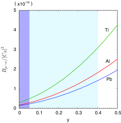
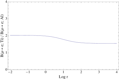
Among the above models, the scalar model suffers from the uncertainty in the parameter. We show in Fig. 1 the -parameter dependence of the conversion branching ratio. The uncertainty is quite large if we take the conservative range, .
Each of the above classes of models has only one free parameter – the ratio of the dominant effective coupling over the square of the new physics scale. It is clear, then, that the single-operator dominance hypothesis makes parameter-free predictions for ratios of LFV branching fractions and therefore it can be tested so long as two LFV rates are measured. We will discuss how well one can distinguish models in the presence of the theoretical uncertainties.
3.2 vs conversion
If and conversion in at least one target nucleus are observed, this immediately opens up the possibility to test the Dipole dominance model. In fact, in this model the ratio
| (47) |
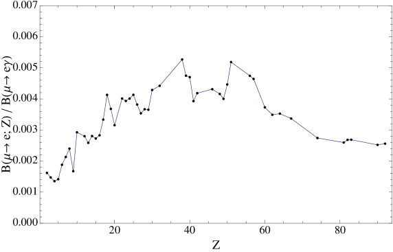
is entirely fixed by the overlap integrals [6], which are essentially free of theoretical uncertainty. is predicted to scale as and we plot it in Fig. 2. We omit from the plot the points corresponding to , , and , as data on the nucleon densities are either obtained from quite old experiments or not well established [24]. Any deviation from the pattern shown in Fig. 2 would imply the presence of scalar or/and vector contributions. In order to disentangle these possibilities, one needs to study the target dependence of the conversion rate.
3.3 Target dependence of conversion
In principle, any single-operator model can be tested with two conversion rates, even if is not observed. To illustrate this point, we update the analysis of Ref. [6] and plot in Fig. 3 the conversion rate (normalized to the rate in Aluminum) as a function of the of the target nucleus, for the four classes of single-operator models defined above. Compared to Ref. [6], the novelty here is the inclusion of a second vector model ().
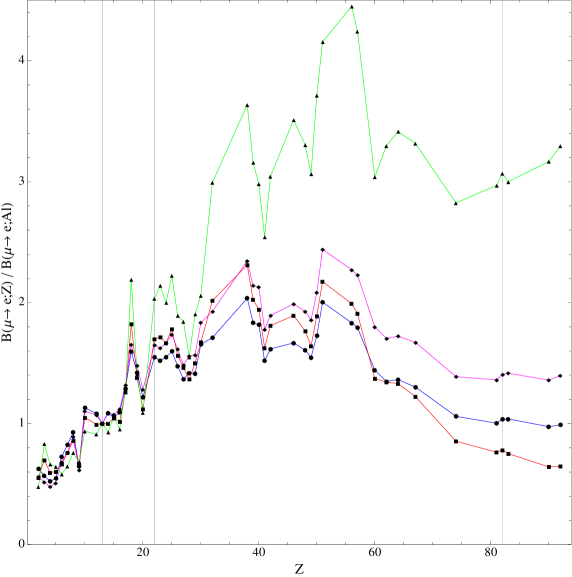
The results of Fig. 3 show some noteworthy features. First, we note the quite different target dependence of the conversion rate in the two vector models considered. This can be understood as follows: in the case of the model, the behavior in Fig. 3 simply traces the -dependence of (the photon only couples to the protons in the nucleus). On the other hand, in the case of the model, the boson couples predominantly to the neutrons in the nucleus and the target dependence of the ratio generates the behavior observed in Fig. 3.
Next, let us focus on the actual discriminating power of the -dependence. Clearly, the plot shows that the model-discriminating power tends to increase with . This is a simple reflection of the fact that the whole effect is of relativistic origin and increases in heavy nuclei. So in an ideal world, in order to maximize the chance to discriminate among underlying models, one would like to measure the conversion rate in a light nucleus, say Aluminum or Titanium, as well as in a large- nucleus, like Lead or Gold. This simplified view, however, has to be confronted both with theoretical uncertainties and the actual experimental feasibility. Concerning the uncertainties, a simple analysis shows that the dominant uncertainty coming from the scalar matrix elements almost entirely cancels when taking ratios of conversion rates (even using the conservative range for the strange scalar density matrix element). Moreover, in the large- tail of the plot, some residual uncertainty arises from the input on the neutron density profile. When polarized proton scattering data exists, the uncertainty on the ratios of conversion rates becomes negligible. This point is illustrated by Table 1, where we report the detailed breakdown of uncertainties in the ratios and . For other targets, the uncertainty induced by neutron densities never exceeds [6]. The conclusions of this exercise are that:
-
•
The theoretical uncertainties (scalar matrix elements and neutron densities) largely cancel when we take a ratio.
-
•
As evident from Fig. 3, a realistic discrimination among models requires a measure of at the level of or better, or alternatively a measure of at the level. These are two cases that well represent the trend in light and heavy target nuclei.
| 1.70 0.005y | 1.55 | 1.65 | 2.0 | |
| 0.69 0.02 | 1.04 | 1.41 | 2.67 0.06 |
4 Testing the two-operator dominance hypothesis
In the last section we have discussed how to test the hypothesis of a single operator dominance, and how to discriminate among different single-operator dominance models. If the single operator dominance hypothesis fails, one is lead to consider next simplest case, namely the two-operator dominance models, defined by the assumption that only two underlying operators have appreciable coefficients. Each model is characterized by two parameters, the effective strength of one of the two operators and the ratio of the effective couplings of the two dominant operators. This class of models can be tested so long as two double ratios of LFV rates are available (three LFV measurements!).
For the sake of illustration, we will consider the following three two-operator models: Dipole-Scalar, Dipole-Vector(Z) and Scalar-Vector(Z). We consider both the case of constructive and destructive interference among the two dominant operators, assuming that the ratio of Wilson coefficients is real (a relative phase can be included but it would unnecessarily complicate the analysis at this early stage). In order to test this class of models, one has to assume that at least three LFV processes have been observed, so one can construct two independent double ratios that are entirely determined by the single parameter . In models involving the Dipole operator among the dominant terms (such as Dipole-Scalar and Dipole-Vector) the three observables could be (i) and conversion in two different targets; or (ii) conversion in three different targets. In models that do not involve a Dipole term (such as Scalar-Vector), only the possibility (ii) above is available. As representative target nuclei, we have chosen aluminum (), titanium (), and lead ().
4.1 Dipole-Scalar
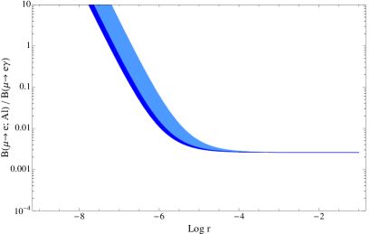
In terms of the parameters introduced in Section 3.1, this model is defined by and . The single-operator models are recovered in the limiting cases (scalar) and (dipole) 333We consider here the case in which dipole and scalar operators produce outgoing lepton with definite chirality (L or R). If both chiralities are allowed, then in principle and one more parameter has to be introduced in the analysis.. Note that in this particular case the asymptotic dipole regime is reached already for because of the peculiar normalization of the scalar operators (suppressed by the factor ).
(a)
(b)

(c)
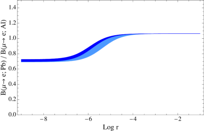
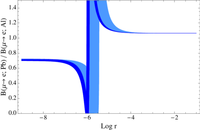
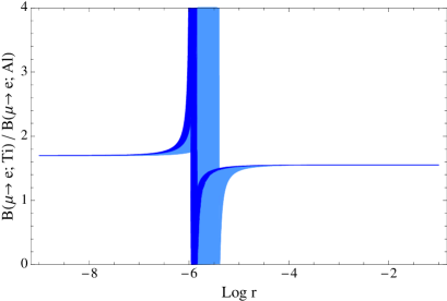
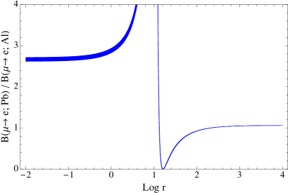
We illustrate the features of this model in Figs. 4 and 5, which correspond to positive and negative sign of the ratio , respectively. Panel (a) shows the behavior of versus the parameter , while panels (b) and (c) show the ratios and , respectively. In panels (a) and (c) the curve is widened in the interference region by the uncertainty in the scalar form factors. The dominant uncertainty comes from the input parameter , characterizing the strangeness content of the nucleon. On the other hand, the ratio is affected not only by the uncertainty in the scalar form factors, but also by the uncertainty induced in the overlap integral by the neutron density in Pb. The width of the bands in panel (b) is determined by the most conservative combination of two kind of uncertainties.
In all panels the wide band corresponds to the range , while the narrow band corresponds to the range . This illustrates the effect of current and future hadronic uncertainties on the process of extracting information on short distance LFV couplings. The prominent feature in Fig. 5 is induced by the destructive interference dipole and scalar amplitudes.

(a)
(b)
(c)
4.2 Dipole-Vector
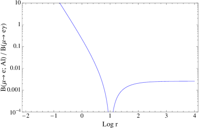
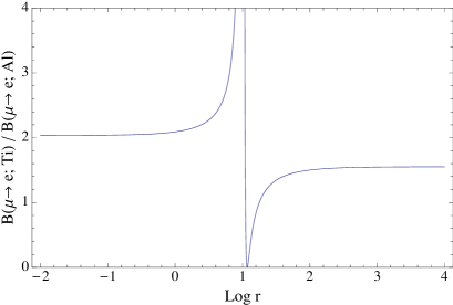
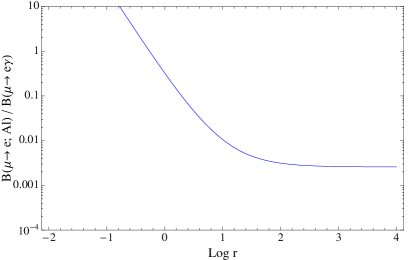
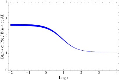
In terms of the parameters defined in Section 3.1, this model is defined by and . The single-operator models are recovered in the limiting cases (vector) and (dipole). In figures 6 and 7 we plot the ratios (panel (a)), (panel (b)), and (panel (c)) versus the parameter . Figures 6 and 7 correspond to positive and negative sign of the ratio , respectively. Within this model, the only source of uncertainty arises from the vector overlap integral , sensitive to the neutron density in Pb. This uncertainty is quantified by the thickness of the band in panel (b).
(a)
(b)
(c)
(a)
(b)
(c)
4.3 Scalar-Vector
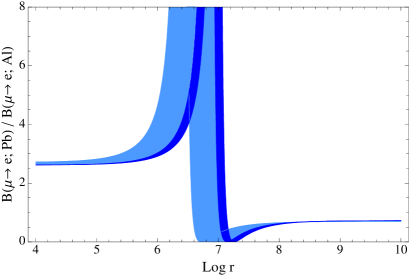
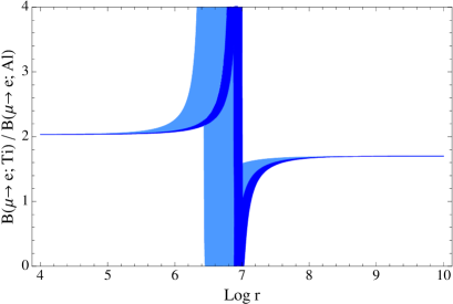
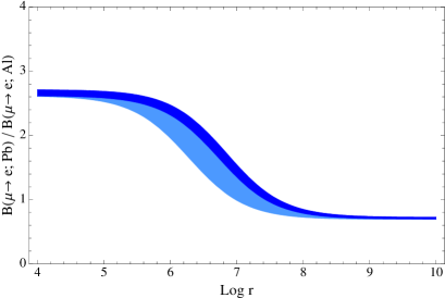
In terms of the parameters defined in Section 3.1, this model is defined by and . The single-operator models are recovered in the limiting cases (vector) and (scalar). Since the Dipole term is assumed to be subdominant, in this case we include in the analysis only the ratios and , shown in panels (b) and (c) of Figures 8 and 9 (for positive and negative values of , respectively). While the ratio is affected only by the uncertainty in , the ratio is affected also by the uncertainty in the Pb neutron density (through the overlap integrals). The width of the bands in the plots is determined by the most conservative combination of two kind of uncertainties.
In all panels the wide band corresponds to the range , while the narrow band corresponds to the range . As in the case of the Dipole-Scalar model, the bands illustrate the effect of current and future hadronic uncertainties on extracting short distance LFV couplings.
(b)
(c)
(b)

(c)
We conclude this section by summarizing what one could learn about the two-operator dominance models in the case that two double ratios of LFV rates could be measured experimentally. Our exercise shows that:
-
•
The current theoretical uncertainty on the strange content of the nucleon prevents a realistic test of the two-operator models involving the Scalar amplitude. The range induces uncertainties of up to one order of magnitude in the relevant double ratios in the interference region (thick bands in all plots above). However, the uncertainty within reach of lattice QCD calculations will remove this obstacle in the coming years (this is illustrated by the thin bands in all plots above).
-
•
Testing and discriminating among two-operator dominance models requires an experimental precision on the LFV rates that is comparable to the one needed to test the single operator models.
5 Application to a SUSY model
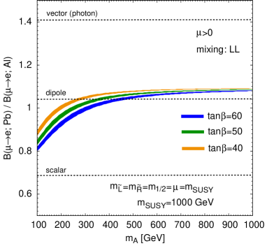
An example of the two-operator dominance model is given by a SUSY scenario with flavor mixing in the left-handed sleptons. Such a mixing, for example, can be induced from the Yukawa interaction in the see-saw model. As it is shown in Ref. [22], the scalar operator originated from the Higgs-boson-exchange diagrams can be sizable in this model if is large and the heavy Higgs boson is relatively lighter than the other SUSY particles. The ratio can therefore be enhanced in such a parameter region, while the ratio can show substantial deviations from the dipole-dominance value.
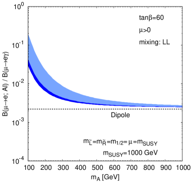

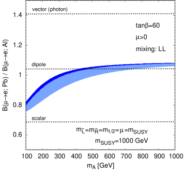
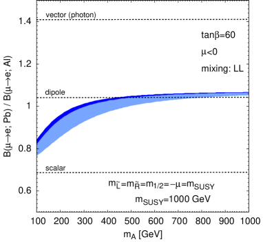
In Fig. 10 we show the pseudoscalar-Higgs mass () dependence of the ratio for (left) and (right). We have taken the common mass ( TeV) for the slepton masses, the universal gaugino mass at the GUT scale, and the Higgsino mass parameter, and we fixed . Since the scalar operator does not decouple in the limit, we see the enhancement in the small region. The light (dark) shaded regions correspond to the conservative (optimistic) range of the parameter, (). Within the same framework, the ratio is shown in Fig. 11.
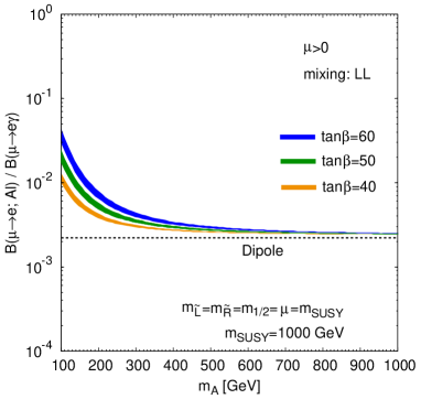
In both cases, the theoretical uncertainty becomes significant as the scalar operator gets important. In the context of this explicit supersymmetric model, a precise determination of the parameter is quite important in order to extract information on the underlying model parameters. To illustrate this even more explicitly, in Fig. 12 we show for the dependence of (left) and (right) for different values of . In these plots, only the small uncertainty window is reported (), to illustrate the enhanced discriminating power.
6 Conclusions
In this work we have investigated whether the target-dependence of -to- conversion rate can be exploited to discriminate among underlying dynamical mechanisms of lepton flavor violation, once one takes into account realistic hadronic and nuclear uncertainties. The major source of theoretical uncertainty arises from the nucleon matrix element of the strange quark scalar density. This is expressed in terms of the parameter (see Eq. 32), which we have varied within two ranges reflecting the current uncertainty () and the projected uncertainty within reach of lattice QCD calculations ().
In order to assess the model discriminating power of a combined phenomenological analysis of and conversion on different target nuclei, we have defined four classes of models, in which only one underlying short distance operator dominates over all the others (Dipole, Scalar, Vector () and Vector ()). Ratios of LFV branching fractions can be used to test the various models. The single-operator hypothesis can be tested with at least one ratio (two LFV measurements), while the two-operator models, where two operators have comparable strength and interfere, can be tested with at least two ratios (three LFV measurements).
Our conclusions are encouraging: the theoretical uncertainties (even at the current level) are not an issue in testing the single-operator dominance model, as they largely cancel when we take ratios of different conversion rates. On the other hand, the current uncertainty prevents meaningful tests of two-operator models involving the Scalar operator, as it produces errors of up to one order of magnitude in the double ratios in the interference region. However, with the anticipated reduced lattice error on the strange content of the nucleon, this will not be an issue in the future. We have illustrated these main conclusions also in the context of a suprsymmetric model.
Having established that the hadronic uncertainties will not be a limiting factor, we can ask how well one should measure the LFV rates in order to discriminate the underlying models. Fig. 3 shows that a realistic discrimination among single-operator models requires a measure of the ratio of conversion rates in light nuclei (such as ) at the level of or better. Alternatively, one would need to measure the ratio of conversion rates in a heavy and light element (such as ) at the level. Similar accuracy is required on the experimental side to be sensitive to interference effects when more than one operator is at work. Whether these challenging benchmark numbers can be reached in the future round of experiments [25, 26] depends on many issues, including the value of the branching fraction themselves (we are concerned here with ratios). Nonetheless, we hope that our results will stimulate further experimental efforts towards measurements of and -to- conversion and consideration of various options for target nuclei.
Acknowledgments – We thank Satoshi Mihara for useful exchanges on the experimental aspects of -to- conversion and Tetsuya Onogi for useful comments on the sigma term. V. C. thanks the KEK theory group for its hospitality and support, as well as the Institute for Nuclear Theory at the University of Washington for its hospitality and the Department of Energy for support during the completion of this work. Y. O. is supported in part by the Grant-in-Aid for Science Research, Ministry of Education, Culture, Sports, Science and Technology, Japan, No. 16081211 and by the Grant-in-Aid for Science Research, Japan Society for the Promotion of Science, No. 20244037. P. T. has been supported in part by the theory group at LANL (during her visit), by a grant from the Spanish Ministry of Science and Innovation (AP2006-04522), as well as by the EU MRTN-CT-2006-035482 (FLAVIAnet), by MEC (Spain) under grant FPA2007-60323, and by the Spanish Consolider-Ingeino 2010 Programme CPAN (CSD2007-00042).
References
- [1] M. L. Brooks et al. Phys. Rev. Lett. 83, 1521 (1999).
- [2] U. Bellgardt et al. Nucl. Phys. B299, 1 (1988).
- [3] W. Bertl et al. PSI annual report, p.9 (2002) (unpublished).
- [4] C. Dohmen et al. Phys. Lett. B317, 631 (1993).
- [5] W. Honecker et al. Phys. Rev. Lett. 76, 200 (1996).
- [6] R. Kitano, M. Koike and Y. Okada, Phys. Rev. D 66, 096002 (2002) [Erratum-ibid. D 76, 059902 (2007)] [arXiv:hep-ph/0203110].
- [7] O. U. Shanker, Phys. Rev. D 20, 1608 (1979).
- [8] A. Czarnecki, W. J. Marciano and K. Melnikov, AIP Conf. Proc. 435, 409 (1998) [arXiv:hep-ph/9801218].
- [9] T. S. Kosmas, S. Kovalenko and I. Schmidt, Phys. Lett. B 511, 203 (2001) [arXiv:hep-ph/0102101].
- [10] M. A. Shifman, A. I. Vainshtein and V. I. Zakharov, Phys. Lett. B 78, 443 (1978).
- [11] A. Corsetti and P. Nath, Phys. Rev. D 64, 125010 (2001) [arXiv:hep-ph/0003186].
- [12] H. Ohki et al., Phys. Rev. D 78, 054502 (2008) [arXiv:0806.4744 [hep-lat]].
- [13] J. Gasser, H. Leutwyler, M. P. Locher and M. E. Sainio, Phys. Lett. B 213, 85 (1988); J. Gasser, H. Leutwyler and M. E. Sainio, Phys. Lett. B 253, 252 (1991).
- [14] M. M. Pavan, I. I. Strakovsky, R. L. Workman and R. A. Arndt, PiN Newslett. 16, 110 (2002) [arXiv:hep-ph/0111066].
- [15] B. Borasoy and U. G. Meissner, Annals Phys. 254, 192 (1997) [arXiv:hep-ph/9607432].
- [16] M. Procura, T. R. Hemmert and W. Weise, Phys. Rev. D 69, 034505 (2004) [arXiv:hep-lat/0309020]; M. Procura, B. U. Musch, T. Wollenweber, T. R. Hemmert and W. Weise, Phys. Rev. D 73, 114510 (2006) [arXiv:hep-lat/0603001].
- [17] H. Cheng, Phys. Lett. B219, 347 (1989).
- [18] H. Leutwyler, Phys. Lett. B 378, 313 (1996) [arXiv:hep-ph/9602366].
- [19] R. Barbieri and L. J. Hall, Phys. Lett. B 338, 212 (1994) [arXiv:hep-ph/9408406]; R. Barbieri, L. J. Hall and A. Strumia, Nucl. Phys. B 445, 219 (1995) [arXiv:hep-ph/9501334]; J. Hisano, T. Moroi, K. Tobe and M. Yamaguchi, Phys. Lett. B 391, 341 (1997) [Erratum-ibid. B 397, 357 (1997)] [arXiv:hep-ph/9605296].
- [20] F. Borzumati and A. Masiero, Phys. Rev. Lett. 57, 961 (1986); J. Hisano, T. Moroi, K. Tobe and M. Yamaguchi, Phys. Rev. D 53, 2442 (1996) [arXiv:hep-ph/9510309].
- [21] V. Cirigliano, A. Kurylov, M. J. Ramsey-Musolf and P. Vogel, Phys. Rev. D 70, 075007 (2004) [arXiv:hep-ph/0404233].
- [22] R. Kitano, M. Koike, S. Komine and Y. Okada, Phys. Lett. B 575, 300 (2003) [arXiv:hep-ph/0308021].
- [23] J. E. Kim, P. Ko and D. G. Lee, Phys. Rev. D 56, 100 (1997) [arXiv:hep-ph/9701381]; K. Huitu, J. Maalampi, M. Raidal and A. Santamaria, Phys. Lett. B 430, 355 (1998) [arXiv:hep-ph/9712249]; A. Faessler, T. S. Kosmas, S. Kovalenko and J. D. Vergados, Nucl. Phys. B 587, 25 (2000); A. de Gouvea, S. Lola and K. Tobe, Phys. Rev. D 63, 035004 (2001) [arXiv:hep-ph/0008085].
- [24] H. De Vries, C. W. De Jager and C. De Vries, Atom. Data Nucl. Data Tabl. 36, 495 (1987); G. Fricke et al., ibid. 60, 177 (1995).
- [25] Mu2e Collaboration website: http://mu2e.fnal.gov/
- [26] COMET: http://comet.phys.sci.osaka-u.ac.jp/internal/publications/main.pdf