Implicit and explicit solvent models for the simulation of a single polymer chain in solution: Lattice Boltzmann vs Brownian dynamics

Abstract

We present a comparative study of two computer simulation methods to obtain static and dynamic properties of dilute polymer solutions. The first approach is a recently established hybrid algorithm based upon dissipative coupling between Molecular Dynamics and lattice Boltzmann (LB), while the second is standard Brownian Dynamics (BD) with fluctuating hydrodynamic interactions. Applying these methods to the same physical system (a single polymer chain in a good solvent in thermal equilibrium) allows us to draw a detailed and quantitative comparison in terms of both accuracy and efficiency. It is found that the static conformations of the LB model are distorted when the box length $L$ is too small compared to the chain size. Furthermore, some dynamic properties of the LB model are subject to an $L^{-1}$ finite size effect, while the BD model directly reproduces the asymptotic $L\to\infty$ behavior. Apart from these finite size effects, it is also found that in order to obtain the correct dynamic properties for the LB simulations, it is crucial to properly thermalize all the kinetic modes. Only in this case, the results are in excellent agreement with each other, as expected. Moreover, Brownian Dynamics is found to be much more efficient than lattice Boltzmann as long as the degree of polymerization is not excessively large.

I Introduction

The rich variety of conformations which leads to many different intrinsic properties of polymer solutions has continuously drawn considerable interest in soft matter research. Computer modeling is increasingly being used as an integral part of theoretical study, in order to both test existing theories and to trigger the development of new concepts. Furthermore, computer simulations have also become an essential tool in materials research, especially for predicting and understanding the behavior of complex systems, where a complete theory is not available. It has been proven to be an effective and inexpensive way to study these systems. In order to observe large-scale properties, it is crucial to reduce the computational cost by coarse-graining the details of the atomic structure. This is particularly true for polymer systems and studies of their universal static and dynamic properties deGennes79 ; DoiEdwards86 . In this context, using a conventional bead-spring chain model to represent a polymer molecule in Molecular Dynamics (MD) simulations is usually sufficient KremerGrest90 ; PierleoniRyckaert92 ; SmithRapaport92 ; DuenwegKremer93 ; Binder95 . In the case of dilute and semidilute polymer solutions, a correct model also needs to take into account the effect of solvent molecules. This effect is two-fold: On the one hand, the good solvent quality results in swelling of the random coil; on the other, the solvent-mediated long-range dynamic correlations between different segments of the chain, known as hydrodynamic interactions (HI), significantly influence the dynamical behavior deGennes79 ; DoiEdwards86 ; SuntharPrakash06 . In the present methodological study, we focus on the dilute regime which is theoretically most thoroughly understood.

In order to capture hydrodynamic interactions in MD simulations, the solvent particles need to be incorporated explicitly. Typically, the number of solvent particles required for such a model is of the order of thousands even for a short chain. Although such studies are feasible DuenwegKremer93 , they are rather inefficient, for this reason. Therefore, a more coarse-grained description of the solvent is highly desirable. Two complementary approaches have been developed to do this. “Mesoscopic” methods keep the solvent degrees of freedom, but describe them in a simplified fashion. These include Dissipative Particle Dynamics (DPD) HoogerbruggeKoelman92 ; Schlijperetal95 ; EspanolWarren95 ; Marshetal97 ; GrootWarren97 ; Espanol98 ; Pagonabarragaetal98 , Multi–Particle Collision Dynamics (MPCD) MalevanetsKapral99 ; LeeKapral06 ; Gompper09 , and lattice Boltzmann (LB) Benzietal92 ; Ladd94a ; Ladd94b ; ChenDoolen98 ; Succi01 ; LaddVerberg01 ; DuenwegLadd09 ; AhlrichsDuenweg98 ; AhlrichsDuenweg99 ; Adhikarietal05 ; Duenwegetal07 . These approaches are typically one to two orders of magnitude faster than MD AhlrichsDuenweg99 . Conversely, Brownian Dynamics (BD) simulations ErmakMcCammon78 ; Jendrejacketal02 ; LiuDuenweg03 ; Prabhakaretal04b ; SuntharPrakash05 remove the solvent degrees of freedom completely, and take their effect into account via non-trivial long-range dynamic correlations in the stochastic displacements. This is possible due to the time scale separation between the fast solvent motion and the slow conformational polymer degrees of freedom. Since the number of degrees of freedom is reduced drastically, the method has the potential to save CPU time by additional several orders of magnitude, in particular in the dilute limit. However, a simple implementation of the correlations ErmakMcCammon78 leads to an algorithm which scales like $O(N^{3})$, where $N$ is the number of Brownian particles, and therefore becomes infeasible as soon as $N$ exceeds a few hundred LiuDuenweg03 . It is therefore very important to treat HI by means of Fixman’s algorithm Fixman86 (scaling roughly as $O(N^{2.25})$), which we do in the present study. The recently introduced method by Geyer and Winter GeyerWinter08 would reduce the necessary CPU effort by roughly one additional order of magnitude for typical chain lengths, and exhibit a more favorable scaling ($O(N^{2})$). However, it is based upon an inexact approximation of the hydrodynamic correlations that cannot be improved systematically (in contrast to Fixman’s method). For this reason, this algorithm was not implemented.

None of these approaches is sufficient to reach $N\sim 10^{3}\ldots 10^{4}$; this latter goal is only attainable by the implementation of very recent “superfast” BD algorithms based upon Fast Fourier Transforms BanchioBrady03 ; Saintillanetal05 ; Hernandez-Ortizetal07 . These latter algorithms scale as $N^{1+x}\log N$, where the exponent $x$ depends on the details of the underlying physics, and is usually substantially smaller than unity. These methods require the study of a confined system, and hence are not used in the present study.

While the advantages and disadvantages of the methods are well-known in general terms (and have resulted in differing methodological preferences in different groups of researchers), not much is known quantitatively in terms of a clear comparison of computational efficiency. The present paper aims at partly filling this gap.

Recently, one of the present authors AhlrichsDuenweg98 ; AhlrichsDuenweg99 has proposed a new mesoscopic method for simulating polymer-solvent systems. The solvent is represented by a fluid on a grid, simulated via the lattice Boltzmann approach, while the motion of the polymer chain is governed by a continuous MD model. The two parts are coupled by a simple dissipative force. The lattice Boltzmann (LB) method was originally developed to simulate hydrodynamics on a grid Benzietal92 ; ChenDoolen98 . It has been shown that the LB method is a fast and effective method for simulating fluid flows, which has the same speed and accuracy as other Navier-Stokes solvers Benzietal92 ; Ladd94a ; Martinezetal94 ; Ladd94b . Ladd Ladd94a ; Ladd94b successfully applied the LB method to colloidal systems (originally with a conservative coupling) and showed that the CPU cost scales linearly with the number of particles. Moreover, he showed how fluctuations can be incorporated into the LB model, which is essential in order to investigate Brownian motion Ladd94a . This procedure has recently been refined and improved Adhikarietal05 ; Duenwegetal07 . The dissipative coupling method AhlrichsDuenweg98 ; AhlrichsDuenweg99 was thoroughly tested by applying it to a single polymer chain in solution, for which the data of a previous MD simulation DuenwegKremer93 were available, and whose parameters were used as an input for the mesoscopic model.

In this work, we study the dynamics of a single chain in a solvent to compare the predictions of the explicit solvent model via the LB method with the predictions of the implicit solvent model by BD simulations. Many recent simulation studies have investigated very similar systems, using various mesoscopic solvent models like MPCD mussawisade , DPD Jiangetal07 , direct solution of the Navier-Stokes equation giupponi , and smoothed DPD litvinov . These studies were mainly done in order to test and verify the validity of the chosen mesoscopic simulation approach. Meanwhile it is fair to say that a single chain in solution is a standard benchmark test bed for mesoscopic simulation methods, the necessary condition for passing being the correct reproduction of the Zimm scaling laws within the limitations of finite chain length and finite solvent volume. The present study, however, aims directly at a quantititave comparison between two different methods, and therefore it is crucial that that the underlying polymer model is exactly identical for both methods. This is the reason why the data of Refs. mussawisade ; Jiangetal07 ; giupponi ; litvinov , though all exhibiting essentially the same physics, are of no direct relevance for the present investigation, since all of them employ slightly different polymer models, and simulate solvents with somewhat different viscosities. One very recent study by Ladd et al. laddcomparison has done a rather similar comparison between LB and BD, and arrived at similar conclusions; the present paper should be viewed as a complementary study that puts some more emphasis on the issue of computational efficiency.

After introducing the models, we show how to map the input parameters of the hybrid model onto the input values of the BD model to directly compare the predicted quantities (Sec. II). Section III then confirms the expected physical equivalence of the two approaches in terms of comparing static and dynamic data. Furthermore, this section also presents our comparison on the numerical cost or benchmark data for both methods. Finally, in Sec. IV we summarize the results and give our conclusions.

II Molecular model and simulation methods

II.1 Molecular model

In this work, a polymer molecule is represented by a conventional bead-spring chain model, which consists of $N$ beads that are connected via $N-1$ finitely extensible nonlinear elastic (FENE) massless springs. The Lennard-Jones potential, which acts between all monomers, is used to model the excluded volume (EV) effect. The two potentials $V_{\text{FENE}}$ and $V_{\text{LJ}}$ are given by the expressions

$$V_{\text{FENE}} = -\frac{k_{\text{FENE}}R^{2}_{0}}{2}\ln\left(1-\left(\frac{r}{R_{0}}\right)^{2}\right),$$ (1)

$$V_{\text{LJ}} = 4\epsilon\left(\frac{\sigma^{12}}{r^{12}}-\frac{\sigma^{6}}{r^{6}}+\frac{1}{4}\right),\quad r\leq 2^{1/6}\sigma,$$ (2)

where $r$ is the bead-bead distance, $k_{\text{FENE}}$ is the spring constant and $R_{0}$ the maximum extension of the bond. $\epsilon$ and $\sigma$ are the energy and length parameters of the Lennard-Jones potential, respectively.

II.2 The lattice Boltzmann (LB) method

In this method, the evolution of the LB variables $n_{i}$ is governed by the following lattice Boltzmann equation Benzietal92 ; Succi01 ; DuenwegLadd09 :

$$n_{i}(\mathbf{r}+\mathbf{c}_{i}\Delta\tau,t+\Delta\tau)=n_{i}(\mathbf{r},t)$$

$$+ \sum_{j=1}^{b}L_{ij}\left(n_{j}(\mathbf{r},t)-n_{j}^{\text{eq}}(\rho,\mathbf{u})\right)+n^{\prime}_{i}(\mathbf{r},t).$$

The variable $n_{i}(\mathbf{r},t)$ is the (partial) fluid mass density at grid site $\mathbf{r}$ at time $t$, corresponding to the discrete velocity $\mathbf{c}_{i}$. $\Delta\tau$ is the time step, and the lattice spacing is denoted by $a$. The small set of velocities $\mathbf{c}_{i}$ ($i=1,\ldots,b$, where the value of $b$ depends on the details of the model) is chosen such that $\mathbf{c}_{i}\Delta\tau$ is a vector leading to the $i$th neighbor on the grid. $L_{ij}$ is a collision operator for dissipation due to fluid particle collisions, such that the populations always relax toward the local pseudo-equilibrium distribution $n_{j}^{\text{eq}}$ that depends on the local hydrodynamic variables $\rho=\sum_{i}n_{i}$ (the total mass density) and $\mathbf{u}=\sum_{i}n_{i}\mathbf{c}_{i}/\sum_{i}n_{i}$ (the local flow velocity). The collision process is constructed in such a way that it conserves both $\rho$ and $\mathbf{u}$. $n^{\prime}_{i}(\mathbf{r},t)$ is the stochastic term, which is essential in order to simulate thermal fluctuations that drive Brownian motion.

The local pseudo-equilibrium distribution can be represented as a second-order expansion of the Maxwell-Boltzmann distribution, given by Succi01

$$n_{i}^{\text{eq}}(\rho,\mathbf{u})=\rho w_{c_{i}}\left(1+\frac{\mathbf{c}_{i}\cdot\mathbf{u}}{c^{2}_{\text{s}}}+\frac{(\mathbf{c}_{i}\cdot\mathbf{u})^{2}}{2c^{4}_{\text{s}}}-\frac{u^{2}}{2c^{2}_{\text{s}}}\right),$$ (4)

where $w_{c_{i}}$ are a set of weight factors, which depend on the sublattice $i$ (i. e. the magnitude of $\mathbf{c}_{i}$) and $c_{\text{s}}=\sqrt{1/3}(a/\Delta\tau)$ is the speed of sound. In this work, we have used the algorithm proposed in Ref. AhlrichsDuenweg99 , however, with the modification that the original 18-velocity model (D3Q18) was replaced by the D3Q19 19-velocity model Succi01 . The set of $\mathbf{c}_{i}$ consists of the particle being at rest, the 6 nearest and 12 next-nearest neighbors on a simple cubic lattice. The magnitudes of the velocities corresponding to these three sets of particles are $c_{i}=\left|\mathbf{c}_{i}\right|=0,a/\Delta\tau$, and $\sqrt{2}a/\Delta\tau$, respectively. The weight factors for the D3Q19 model are $w_{0}=1/3$, $w_{1}=1/18$ and $w_{\sqrt{2}}=1/36$.

The early model of Ref. AhlrichsDuenweg99 only considered the thermalization of modes related to the viscous stress tensor. It is important to note that even though this procedure is correct in the hydrodynamic limit, it provides poor thermalization on smaller length scales Adhikarietal05 . Adhikari et al. Adhikarietal05 have shown that by applying thermalization to all nonconserved modes one gets a significantly improved numerical behavior at short scales; the theoretical background is now thoroughly understood Duenwegetal07 ; DuenwegLadd09 . In this work, we have also investigated the effects of thermalization of the kinetic modes on various dynamic properties.

The coupling to the beads is done via simple interpolation of the flow velocity from the surrounding sites, and by introducing a phenomenological Stokes friction coefficient $\zeta_{\text{bare}}$ of the beads. This gives rise to a friction force on the particles, plus a Langevin force that balances the frictional losses. The total momentum is conserved by subtracting the corresponding momentum transfer from the surrounding fluid. It can be shown that this procedure satisfies the fluctuation-dissipation theorem DuenwegLadd09 . For further technical details on this method and its theoretical analysis, we refer the reader to Ref. DuenwegLadd09 .

II.3 Brownian dynamics (BD) simulations

The configuration of a bead-spring chain is specified by the set of position vectors $\mathbf{r}_{i}$ ($i=1,2,\ldots,N$). The time evolution of this configuration is governed by the Itô stochastic differential equation OttingerBook96 ; PrabhakarPrakash04a ; SuntharPrakash05

$$\mathbf{r}_{i}(t+\Delta t)=\mathbf{r}_{i}(t)+\left(k_{\text{B}}T\right)^{-1}\mathbf{D}_{ij}\cdot\left(\mathbf{F}_{j}^{\text{s}}+\mathbf{F}_{j}^{\text{int}}\right)\Delta t$$

$$+\sqrt{2\Delta t}\,\mathbf{B}_{ij}\cdot\mathbf{W}_{j},\quad\quad j=1,2,\ldots,N,$$ (5)

where summation over repeated indices is implied. Here the symbols $\Delta t$, $k_{\text{B}}$, $T$, and $\mathbf{D}_{ij}$ denote the time step, Boltzmann’s constant, the temperature, and the diffusion tensor, respectively, where the latter decribes the hydrodynamic interactions between the beads. The forces $\mathbf{F}_{j}^{\text{s}}$ and $\mathbf{F}_{j}^{\text{int}}$ are the spring and excluded-volume contributions, repectively. $\mathbf{W}_{i}$ are random variables representing a discretized Wiener process, such that $\left<\mathbf{W}_{j}\right>=0$ and $\left<\mathbf{W}_{i}\otimes\mathbf{W}_{j}\right>=\mathbf{1}\delta_{ij}$, where $\delta_{ij}$ is the Kronecker delta and $\mathbf{1}$ is the unit tensor. Finally, the tensor $\mathbf{B}_{ij}$ is related to the diffusion tensor such that $\mathbf{D}_{ij}=\mathbf{B}_{ik}\cdot\mathbf{B}_{jk}^{\text{T}}$ OttingerBook96 .

The frictional properties of the chain and the hydrodynamic interactions between the beads are modeled via the diffusion tensor $\mathbf{D}_{ij}$. Its diagonal elements contain the bead friction coefficient $\zeta=6\pi\eta_{s}d$, where $\eta_{s}$ is the solvent viscosity and $d$ is the Stokes radius of the bead. The off-diagonal elements represent the hydrodynamic interactions via the tensor $\boldsymbol{\Omega}_{ij}$, for which we take the regularized Rotne-Prager-Yamakawa (RPY) tensor RotnePrager69 ; Yamakawa71 with solvent viscosity $\eta_{s}$ and Stokes radius $d$. Taken together, the diffusion tensor is given by

$$\frac{\mathbf{D}_{ij}}{k_{\text{B}}T}=\zeta^{-1}\delta_{ij}\mathbf{1}+\left(1-\delta_{ij}\right)\boldsymbol{\Omega}_{ij}.$$ (6)

Further details can be found in Ref. PrabhakarPrakash04a .

The computationally most intensive part is to determine the matrix $\mathbf{B}_{ij}$. Generally, Cholesky decomposition of $\mathbf{D}_{ij}$ is used to obtain $\mathbf{B}_{ij}$ as an upper (or lower) triangular matrix, and the computational cost for this method scales as $N^{3}$ Fixman86 . Fixman made use of the fact that there are many possibilities to define $\mathbf{B}_{ij}$ as some square-root matrix of $\mathbf{D}_{ij}$, and, noting that it is the vector $\mathbf{B}_{ij}\cdot\mathbf{W}_{j}$ that is required rather than the matrix $\mathbf{B}_{ij}$, applied a truncated Chebyshev polynomial expansion to obtain $\mathbf{B}_{ij}\cdot\mathbf{W}_{j}$ with a lower computational cost, scaling roughly as $N^{2.25}$ Fixman86 . In the present paper, we make use of this accelerated technique as well.

II.4 Unit systems and parameter mapping

For implementation on a computer, physical quantities must be represented in certain units, i. e. in terms of suitable dimensionless ratios. This is typically done by choosing a natural unit system where three independent elementary quantities are set to unity.

In the coupled MD/LB simulation approach, this is usually done by choosing the Lennard-Jones parameters $\epsilon$, $\sigma$, and $\tau$ ($\tau=\sqrt{m\sigma^{2}/\epsilon}$, where $m$ is the mass of the monomer) as the units of energy, length, and time, respectively; this choice enables one to make direct contact with MD simulations with explicit solvent AhlrichsDuenweg99 . Conversely, BD simulations have traditionally PrabhakarPrakash04a ; SuntharPrakash05 used a unit system where one chooses $k_{\text{B}}T$ as the energy unit and $l_{k}=\sqrt{{k_{\text{B}}T}/{k_{\text{FENE}}}}$ as the length unit. This is particularly useful for the simulation of pure Gaussian (harmonic) chains where the interaction potential has neither an energy scale nor a length scale built in. The time unit in BD simulations is usually chosen as $\tau_{k}=\zeta/(4k_{\text{FENE}})$.

Of course, a meaningful comparison of results requires that all data are represented in one common unit system. At this point, one realizes that this is less straightforward than one might think at first glance. While the conversion of length and energy units is trivial, and directly facilitated by the fact that both methods use the same molecular model for the polymer chain, and perform the simulations at the same temperature, the conversion of time units is not. This is so because of the different time scales underlying the basic updating algorithms: The MD/LB method is based upon simulating the system on inertial time scales, while BD focuses directly on the larger diffusive time scales. This is directly reflected by the occurence of the intertial parameter $m$ (monomer mass) in the MD/LB time unit, which does occur in the BD model, and the diffusive parameter $\zeta$ (monomer friction constant) in the BD time unit. It is important to notice that $\zeta$ is not an input parameter to the MD/LB model. Rather, one needs to carefully distinguish between the short-time friction coefficient $\zeta_{\text{bare}}$ that is indeed an input parameter — it describes the Stokes coupling of the monomer to the LB fluid in its immediate vicinity — and the long-time friction coefficient $\zeta_{\text{eff}}$ describing the particle’s long-time response that is modified by solvent backflow effects. It is this latter parameter that must be identified with the BD $\zeta$, and it is esentially an output parameter. Fortunately, the relation between $\zeta_{\text{bare}}$ and $\zeta_{\text{eff}}$ is well understood — Ahlrichs and Dünweg AhlrichsDuenweg99 ; DuenwegLadd09 have shown that

$$\frac{1}{\zeta_{\text{eff}}}=\frac{1}{\zeta_{\text{bare}}}+\frac{1}{g\eta_{s}a},$$ (7)

where $g$ is a numerical prefactor and $a$ is some measure for the range of interpolation to the surrounding lattice sites. For linear interpolation to the nearest sites, one finds $g\approx 25$, if $a$ is the LB lattice spacing. For highly accurate results, one should also take into account a small correction for the finite size of the simulation box DuenwegLadd09 ; this has however not been done in the present paper. Rather, we took the mapping determined in Ref. AhlrichsDuenweg99 to calculate $\zeta_{\text{eff}}$ from $\zeta_{\text{bare}}$ and identified this with the $\zeta$ parameter of the BD calculations. Although the physical mapping done in this way is essentially correct, it is important to notice that this aspect introduces a certain amount of numerical inaccuracy when it comes to quantitative comparisons.

Given the fact that it is intrinsically impossible to run the two simulations with the same unit system, we chose to keep the previously established systems of the two respective methods, and to map the results a posteriori by the procedure outlined above. Furthermore, we chose to present all results in MD/LB units. Technically, this means that for length and time unit conversions we need to set $\bar{l}\sigma=l^{*}l_{k}$ and $\bar{t}\tau=t^{*}\tau_{k}$, where the “*” superscript denotes BD non-dimensionalization, while “-” denotes a non-dimensionalization for MD/LB. The corresponding factors for the conversion from BD to MD/LB units are then trivially found to be

$$\frac{\sigma}{l_{k}} = \left(\frac{\bar{k}_{\text{FENE}}\epsilon}{k_{\text{B}}T}\right)^{1/2},$$ (8)

$$\frac{\tau}{\tau_{k}} = \frac{4\bar{k}_{\text{FENE}}}{\bar{\zeta}_{\text{eff}}};$$ (9)

note that $\bar{k}_{\text{FENE}}$ and $\bar{\zeta}_{\text{eff}}$ are $k_{\text{FENE}}$ and $\zeta_{\text{eff}}$ in non-dimensional MD/LB units, respectively, while the ratio $k_{B}T/\epsilon$ is just the non-dimensionalized temperature in MD/LB units.

The dimensionless hydrodynamic interaction parameter $h^{*}$ used in the BD simulations is essentially a non-dimensionalized Stokes radius. We thus find

$$h^{*}\sqrt{\pi}l_{k}=d=\frac{\zeta_{\text{eff}}}{6\pi\eta_{s}}=\frac{\bar{\zeta}_{\text{eff}}\sigma}{6\pi\bar{\eta_{s}}},$$ (10)

or

$$h^{*}=\frac{\bar{\zeta}_{\text{eff}}}{6\pi^{3/2}\bar{\eta}}\left(\frac{\bar{k}_{\text{FENE}}\epsilon}{k_{\text{B}}T}\right)^{1/2}.$$ (11)

We therefore parameterized our simulations by first picking simulation parameters for the MD/LB model (which were then directly used for MD/LB), then converting these to BD units using the procedure outlined above, and then running the thus-obtained equivalent BD model. For these latter simulations, a time step size $\Delta t^{*}=0.005$ (in BD units) was found to produce sufficiently accurate results.

II.5 Choice of parameters

The physical input values for the present model are chosen from the benchmark values developed in Ref. AhlrichsDuenweg99 , which have been shown to reproduce the results of a typical pure MD simulation DuenwegKremer93 . As in the comparison between LB and MD simulations, we study a system of a single polymer chain of length $N=32$ monomers immersed in a fluid with temperature $k_{\text{B}}T/\epsilon\ =1.2$, density $\bar{\rho}=0.864$, and kinematic viscosity $\bar{\nu}=2.8$. The lattice spacing $\bar{a}$ is set to unity, which is roughly identical to the bond length; this is necessary to resolve the hydrodynamic interactions on small length scales with sufficient accuracy.

Furthermore, following Ref. AhlrichsDuenweg99 , the coupling parameter $\bar{\zeta}_{\text{bare}}$ was set to $20.8$. The values of the FENE spring potential parameters are $\bar{k}_{\text{FENE}}=7$ and $\bar{R}_{0}=2$. The time step size for the polymer (the MD part of the simulations) is set to $\Delta\bar{t}=0.01$. It should be noted that such a large time step is possible since the inclusion of dissipation and noise lead to a substantial stabilization, compared to purely microcanonical MD. The value of the time step that updates the fluid should be chosen in a way such that the LB variables $n_{i}$ do not become negative too often. Here, we choose $\Delta\bar{\tau}=0.02$, where such a case rarely occurred during the observation time. It is important to mention another free input parameter which governs the time scale for the evolution of hydrodynamic interactions, known as the Schmidt number $Sc=\nu/D_{0}$, where $D_{0}$ is the diffusion constant of the single monomer. This parameter can be set arbitrarily in the LB method by choosing $\nu$ and $D_{0}$ (which can be tuned by choosing $\zeta_{\text{bare}}$) accordingly. Ideally, the value of $Sc$ should be chosen such that hydrodynamic interaction evolves much faster than the diffusion of a monomer. In our case, we have $Sc\approx 32$, which has been shown to result in Zimm-like behavior AhlrichsDuenweg99 ; Jiangetal07 .

For the LB simulations, the polymer chain moves within a cubic box of length $L$ with periodic boundary conditions, while it is drifting freely in an infinite medium for the BD simulations. In order to accurately compare various properties between the two systems, one must understand the effects of the box length $L$ on any observable of interest in the LB simulations. Thus it is essential to only compare quantities under identical conditions (i. e. independent of the box length). Hence various box lengths $L$ ranging from 10 to 35 Lennard-Jones units were investigated; this allows us to extrapolate to the $L\to\infty$ limit.

III Results and discussion

III.1 Static properties

The mean square radius of gyration and the mean square end-to-end distance are given by

$$\left<R^{2}_{\text{g}}\right> = \frac{1}{2N^{2}}\sum_{ij}\left<r^{2}_{ij}\right>,$$ (12)

$$\left<R^{2}_{\text{e}}\right> = \left<\left(\mathbf{r}_{N}-\mathbf{r}_{1}\right)^{2}\right>$$ (13)

with $r_{ij}=\left|\mathbf{r}_{i}-\mathbf{r}_{j}\right|$ being the inter-particle distance.

These two quantities are both related to the number of monomers by the expression

$$\left<R^{2}_{\text{g}}\right>\propto\left<R^{2}_{\text{e}}\right>\propto N^{2\nu},$$ (14)

where $\nu$ is the Flory exponent. For a self-avoiding walk (SAW), the Flory exponent $\nu$ is 0.588 FloryBook88 . In principle, $\nu$ can be obtained from simulations, using the scaling law in Eq. 14. However, this method would require simulations for a wide range of $N$ values. Alternatively, one can use the static structure factor

$$S(k) = \frac{1}{N}\sum_{ij}\left<\exp\left(i\mathbf{k}\cdot\mathbf{r}_{ij}\right)\right>$$ (15)

$$= \frac{1}{N}\sum_{ij}\left<\frac{\sin(kr_{ij})}{kr_{ij}}\right>$$

to obtain $\nu$ much more efficiently.

In the scaling regime $R^{-1}_{\text{g}}\ll k\ll a_{0}$ ($a_{0}$ being a microscopic length of the order of the bond length), a power law relation between the static structure factor and the wave vector $k$ holds:

$$S(k)\propto k^{-1/\nu}.$$ (16)

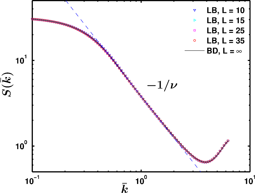
Figure 1 shows the static structure factor as a function of wave vector $k$ for the LB simulations with the presence of thermalization of all modes, and the BD simulations. It can be clearly seen that the values of the static structure factor obtained from the LB simulations are exactly the same as those obtained from the BD simulations, indicating that they have the same static conformations. From Eq. 16, the value of $\nu$ can be extracted from the linear region of the log-log plot of $S(k)$ vs $k$. As expected, the values for $\nu$ obtained via this method are the same for both the LB and the BD simulations, as reported in Table 1. However, they are approximately 5% higher than the asymptotically correct value, which is a consequence of the finite chain length. The results for the mean square radius of gyration and the mean square end-to-end distance in Table 1 further confirm this agreement with regard to static conformations between the two methods. However, at small box length ($L=10$), the results for these static properties for the LB method deviate from their asymptotic values. The discrepancy observed here always arises when the box length is too small compared to the chain size, where the chain is more likely to wrap over itself due to spatial restriction and hence alter its static conformations. We also found that the two versions of LB thermalization (“stresses–only” vs “full” thermalization) yield identical results for the chain conformational statistics. In general, we only quote values obtained for full thermalization, unless indicated otherwise.

The hydrodynamic radius for a single chain in an infinite medium is given by

$$\left<\frac{1}{R_{\text{H}}}\right>_{\infty}=\frac{1}{N^{2}}\sum_{i\neq j}\left<\frac{1}{r_{ij}}\right>.$$ (17)

For a chain in a finite box, as is the case here in the LB method, it has been shown that the hydrodynamic interactions of the chain with its periodic images effectively increases $R_{\text{H}}$ DuenwegKremer93 ; AhlrichsDuenweg99 . In order to account for this finite-size effect, a finite-size correction of order $L^{-1}$ for most dynamic properties, resulting from the slow $r^{-1}$ decay of hydrodynamic interactions, is required DuenwegKremer93 ; AhlrichsDuenweg99 . The results for the infinite-box value $\left<R^{-1}_{\text{H}}\right>_{\infty}$ agree excellently with each other for all simulations (see Table 1). Since the overwrapping effect is more sensitive to large inter-particle distances, it turns out that the deviation in the inverse hydrodynamic radius is too small, for the range of box lengths used, for it to be distinguishable. As can be seen in Table 1, the deviation is more pronounced for the radius of gyration, and even more for the end-to-end distance.

III.2 Dynamic properties

According to dynamic scaling, the longest relaxation time $\tau_{\text{Z}}$ of the chain is, by order of magnitude, identical to the time that the chain needs to move its own size, i. e. $D_{\text{CM}}\tau_{\text{Z}}\sim R^{2}_{\text{g}}$, where $D_{\text{CM}}$ is the diffusion constant of the chain’s center of mass. This leads to a dynamic scaling law $\tau_{\text{Z}}\propto R^{z}_{\text{g}}$, where $z$ is the dynamic scaling exponent. For a chain with hydrodynamic interactions, this relaxation time is known as the Zimm time $\tau_{\text{Z}}$. For this case, $D_{\text{CM}}\propto R^{-1}_{\text{g}}$ in the limit of long chains. This implies that $\tau_{\text{Z}}\propto R^{3}_{\text{g}}$, which gives a dynamic exponent of $z=3$ for models with HI. For the Rouse model (i. e. chains without hydrodynamic interactions), where $D_{\text{CM}}\propto N^{-1}$, one finds a dynamic exponent of $z=2+1/\nu$. These quantities will be referred to in the discussion below.

The mean-square displacement of the chain’s center of mass

$$g_{3}(t)=\left<\left(\mathbf{R}_{CM}(t_{0}+t)-\mathbf{R}_{CM}(t_{0})\right)^{2}\right>$$ (18)

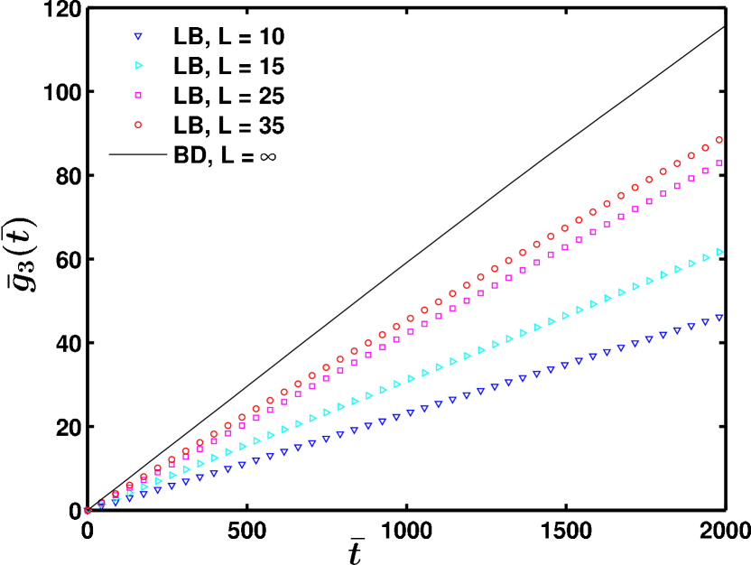
for both methods is depicted in Fig. 2. From the figure, it can be clearly seen that $g_{3}$ strongly depends on the box length $L$ for the LB simulations. Moreover, they seem to converge to the value predicted by the BD simulations ($L=\infty$) in the limit of large $L$. Effects of thermalization of the kinetic modes in LB simulations on this property will be discussed subsequently. The chain’s center of mass diffusion constant $D_{\text{CM}}$ can be determined by the slope of the $g_{3}$ vs $t$ curve, where the relationship $g_{3}(t)=6D_{\text{CM}}t$ holds. By fitting a power law to the simulation data, we obtain the exponents and the diffusion constants shown in Table 1. These exponents support the prediction of simple diffusive behavior ($t^{1}$). Theoretically, one would expect that two diffusive regimes exist: On the one hand, there should be a short-time diffusive regime, corresponding to time scales well below the Zimm time, $t\ll\tau_{\text{Z}}$, but also well above the ballistic regime, $t\gg\tau_{0}$; note that $\tau_{0}>0$ only in the LB case, since the BD equation of motion is overdamped. On the other hand, there should be free diffusion for times $t\gg\tau_{\text{Z}}$. Both these regimes exhibit $t^{1}$ behavior, but with different prefactors, with a smooth crossover around the Zimm time LiuDuenweg03 ; Fixman81 ; Fixman83 . In principle these two different diffusion constants can be obtained via fits to the corresponding regimes. In practice, however, it turns out that the values are very close to each other, and hence the crossover is very smooth LiuDuenweg03 ; Fixman81 ; Fixman83 . Therefore its unambiguous identification is very difficult, i. e. impossible within the resolution of our data.

The mean-square displacement of a single monomer $i$ is given by

$$g_{1}(t)=\left<\left(\mathbf{r}_{i}(t_{0}+t)-\mathbf{r}_{i}(t_{0})\right)^{2}\right>.$$ (19)

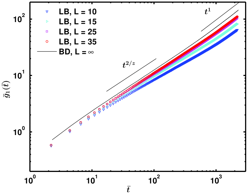
Here, only the two innermost monomers near the center of the chain are evaluated to eliminate end effects; the results are plotted in Fig. 3. The values of $g_{1}$ behave similarly to those of $g_{3}$. In the sub-diffusive time regime, corresponding to the short-time diffusive regime for $g_{3}$, here evaluated between $\bar{t}=20$ and $80$, the scaling behavior $g_{1}(t)\propto t^{2/z}$ is predicted DoiEdwards86 . The corresponding exponents obtained from a power-law fit are listed in Table 1 and indicate a value of $z=2.75$ as $L\rightarrow\infty$. Regardless of the finite-size corrections due to the box length and the effects of thermalization, these values clearly favor the Zimm model compared to the Rouse model, which predicts $g_{1}(t)\propto t^{0.54}$. The deviation from the asymptotic Zimm value $z=3$ (or $g_{1}\propto t^{2/3}$) is mainly a result of finite chain length.

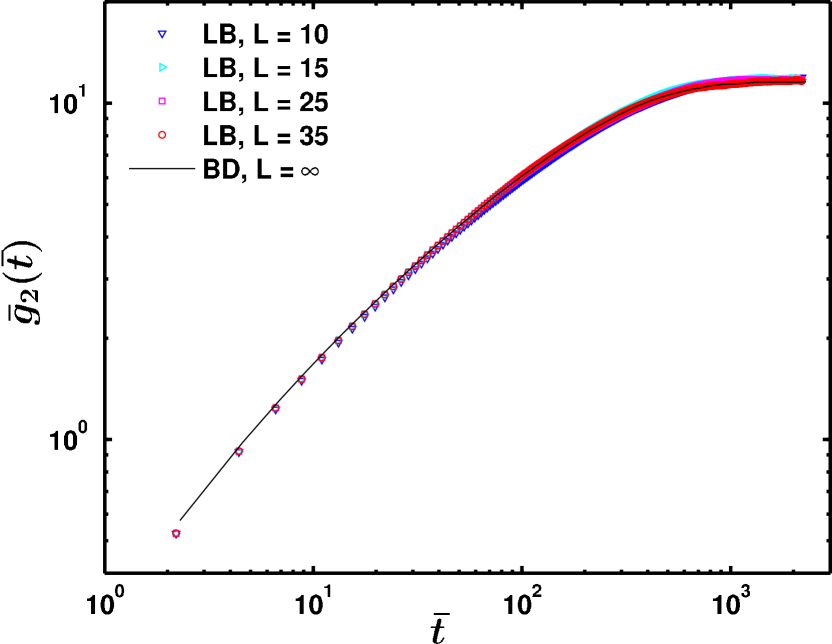
Figure 4 shows the mean-square displacement of a single monomer in the center of mass system (i. e. the two innermost monomers to eliminate end effects)

$$g_{2}(t) = \langle(\left[\mathbf{r}_{i}(t_{0}+t)-\mathbf{R}_{\text{CM}}(t_{0}+t)\right]$$

$$- \left[\mathbf{r}_{i}(t_{0})-\mathbf{R}_{\text{CM}}(t_{0})\right])^{2}\rangle.$$

Interestingly, when viewed within the center of mass system, all the results lie on top of each other, regardless of the box length $L$. This result also holds for LB simulations without full thermalization. This shows that the global center-of-mass motion of the chain is actually the primary contribution to the deviations between LB and BD results. In the data of Fig. 4 this contribution is suppressed: In terms of Rouse modes, only the internal modes remain. For these modes, however, it has been shown AhlrichsDuenweg99 that the HI with the periodic images is much weaker, while the leading-order $r^{-1}$ HI cancels out. Therefore, the corresponding finite-size effect scales as $L^{-3}$ instead of $L^{-1}$, and this is so small that it is invisible in Fig. 4.

Theoretically, these data can also be used for estimating the Zimm time as the time where the crossover to the long-time plateau occurs. However, the crossover is quite extended and smooth, making it difficult to extract. We therefore estimated the Zimm time via

$$\tau_{\text{tr}}=\frac{\left<R^{2}_{\text{g}}\right>}{6D_{\text{CM}}}.$$ (21)

Strictly speaking, this definition is only valid for a single chain in an infinite medium, where there is no finite box size effect. In the presence of finite box size, it becomes the definition for the translational time ($\tau_{\text{tr}}$) rather than the Zimm time: The former is subject to an $L^{-1}$ finite-size effect, due to the strong $L$-dependence of $D_{\text{CM}}$, while the latter, being defined via the relaxation of internal modes, is only subject to an $L^{-3}$ size effect, as discussed above. The translational times obtained from Eq. 21 (as shown in Table 1) are indeed different for different box lengths $L$, as expected. Conversely, the results displayed in Fig. 4 indicate that the systems with different box sizes have (essentially) all the same (internal-mode) Zimm time, since their data all lie on top of each other.

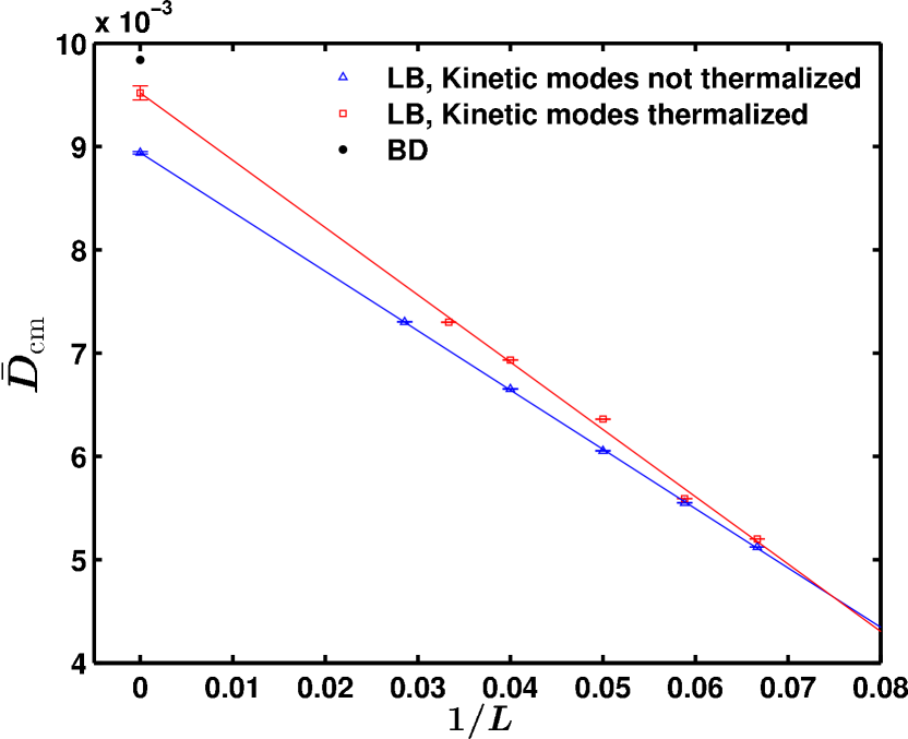
Next, we focus on the leading order $L^{-1}$ finite size correction for the long-time diffusion constant of the chain’s center of mass, $D_{\text{CM}}$. In principle, a plot of $D_{\text{CM}}$ vs $L^{-1}$ should give a straight line for large $L$, and an extrapolation to the limit $L\to\infty$ should yield the same value as predicted by the BD simulations. Figure 5 shows the values of $D_{\text{CM}}$ for the LB simulations with and without thermalization of the kinetic modes at various box lengths $L$ plotted together with the value obtained from the BD simulation at $L=\infty$. It is worth mentioning that the BD value of $D_{\text{CM}}$ can be obtained from the mean square displacement of the chain center of mass or via Fixman’s expression Fixman81 . The latter method has been shown to produce a much more reliable result and is easier to carry out LiuDuenweg03 . The value reported here has been cross checked by both methods and the results are almost the same within error bars. For the LB simulations without thermalization of the kinetic modes, the value of $D_{\text{CM}}$ at the asymptotic limit $L=\infty$ is different from that predicted by the BD simulations by about $9.5\%$. However, when all the kinetic modes in the LB simulations have been thermalized, the deviation in $D_{\text{CM}}$ reduces to $3\%$. This result clearly indicates that it is very important to thermalize all the kinetic modes in order to obtain correct values for dynamic properties.

The reason for the remaining small discrepancy between LB and BD is not completely clear, since there are numerous possible sources. Firstly, it should be noted that the underlying equations of motion are quite different: LB works with inertia, while BD employs overdamped dynamics. This results in different Schmidt numbers $Sc$ and different Mach numbers $Ma$, the latter being defined as the ratio of the flow velocity to the speed of sound: Both are finite in the LB method, while in the BD case they are strictly infinite ($Sc$) and zero ($Ma$), respectively. Furthermore, the shape of the HI function at small interparticle distances is somewhat different for the two methods: In the BD case, we employ the RPY tensor, while the nearest-neighbor interpolation for LB results in a short-range HI that differs somewhat from the RPY tensor (see also the discussion in Ref. DuenwegLadd09 ). Finally, it should be noted that the value of the constant $g$ in Eq. 7, which is crucial for the mapping between the LB friction parameter $\zeta_{\text{bare}}$ and the BD friction $\zeta_{\text{eff}}$, is only known with some numerical inaccuracy. For highly accurate mappings, it is also necessary to include a finite-size correction in the definition of $g$ DuenwegLadd09 ; this was not done in the present study.

In order to examine whether the thermalization of the LB kinetic modes is also important for the internal modes of chain motion, we have performed a Rouse mode analysis. The Rouse modes for a discrete chain are defined as Kopfetal97 ; AhlrichsDuenweg99

$$\mathbf{X}_{p}=\frac{1}{N}\sum_{n=1}^{N}\mathbf{r}_{n}\cos\left[\frac{p\pi}{N}\left(n-\frac{1}{2}\right)\right]$$ (22)

for $p=1,2,\ldots,N-1$.

Within the approximation of the Zimm model, the autocorrelation function of the modes should decay exponentially DoiEdwards86

$$\frac{\left<\mathbf{X}_{p}(t_{0}+t)\cdot\mathbf{X}_{p}(t)\right>}{\left<\mathbf{X}^{2}_{p}\right>}=\exp\left(-\frac{t}{\tau_{p}}\right),$$ (23)

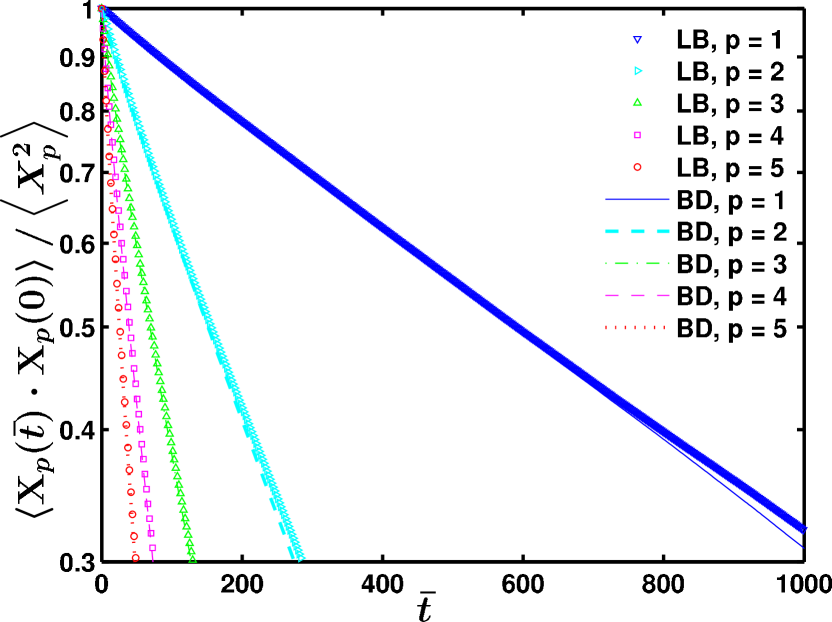
where $\tau_{p}$ is the relaxation of the $p$-th mode. To validate our Rouse mode analysis routine, we have carried out extensive simulations for a (Gaussian) Rouse chain of $N=8$ in the absence of HI and EV; the results for $\tau_{p}$ are in excellent agreement with the analytical predictions DoiEdwards86 . Figure 6 shows the normalized autocorrelation function for $p=1,2,\ldots,5$ for the LB model with box length $L=25$, and the BD model. For nonzero times, there is a small deviation between LB and BD, the latter exhibiting again a slightly faster dynamics. This deviation systematically becomes smaller upon increasing the mode index $p$. Since high mode index means essentially relaxation on a rather small length scale, it is tempting to attribute the deviation to the finite propagation of HI in the LB model, i. e. to retardation effects, or effects of finite Schmidt number, which are more important on large length scales than on small ones. Nevertheless, this hypothesis is not proven.

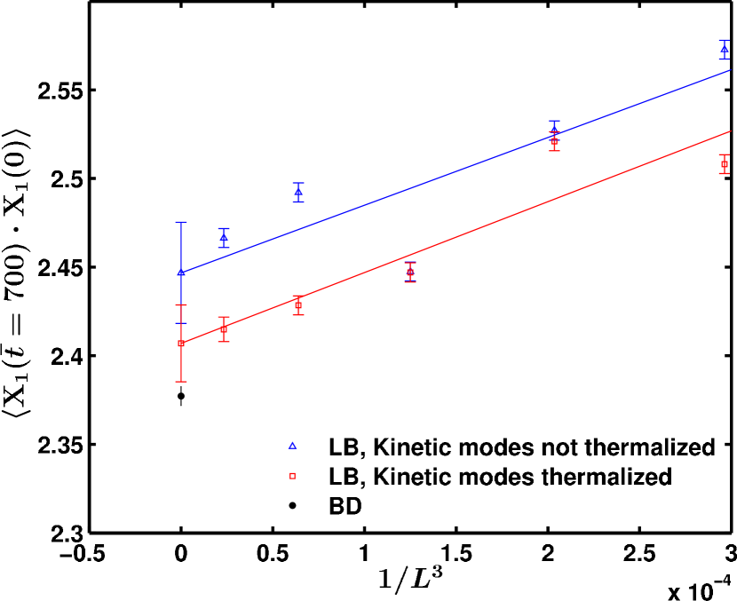
In Ref. AhlrichsDuenweg99 it was shown that the autocorrelation function is only subject to an $L^{-3}$ finite size effect, in contrast to the usual $L^{-1}$ behavior. Figure 7 shows the value of the autocorrelation function of the first Rouse mode $\mathbf{X}_{1}$ at a fixed finite time $\bar{t}=700$, for LB simulations at various box lengths $L$ and BD simulations at $L=\infty$. Within our numerical resolution, the data indeed confirm this $L^{-3}$ finite size effect, both with and without thermalization of the kinetic modes. Furthermore, they demonstrate again that thermalization of all the kinetic modes in LB simulations improves the accuracy of the dynamic properties and brings them closer to the BD prediction: The deviation in the extrapolated limit $L\to\infty$ is reduced from $3\%$ down to $2\%$. The reasons for the remaining discrepancies are probably of the same nature as in the case of $D_{\text{CM}}$.

We have also evaluated the dynamic structure factor, which is defined as

$$S(k,t)=\frac{1}{N}\sum_{ij}\left<\exp\left(i\mathbf{k}\cdot\left[\mathbf{r}_{i}(t)-\mathbf{r}_{j}(0)\right]\right)\right>.$$ (24)

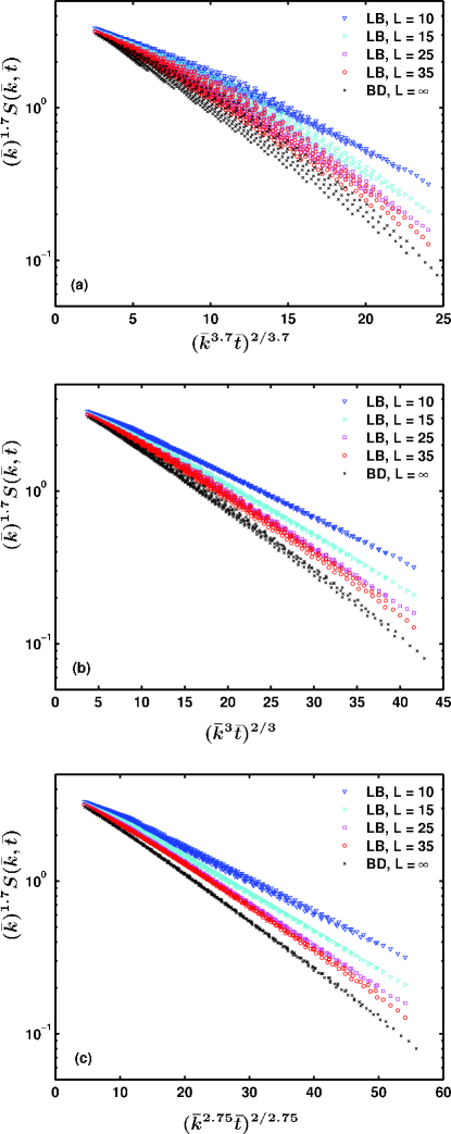
When both wave number and time are in the scaling regime (i. e. $R^{-1}_{\text{g}}\ll k\ll a^{-1}_{0}$ and $\tau_{0}\ll t\ll\tau_{\text{Z}}$), $S(k,t)$ is predicted DoiEdwards86 to exhibit the scaling behavior

$$S(k,t)=S(k,0)f(k^{z}t).$$ (25)

A plot of $S(k,t)k^{1/\nu}$ against $(k^{z}t)^{2/z}$ should collapse to a single curve AhlrichsDuenweg99 . The results for both methods are shown in Fig. 8. The data were restricted to the scaling regime $20<t<80$ and $0.7<k<1.5$. These ranges were obtained from the single monomer mean-square displacement, Fig. 4, and from the static structure factor, Fig. 1, respectively. Here, we particularly focus on adjusting the exponent $z$ such that it would produce the best total data collapse for a chain in an infinite medium (i. e. in the BD model). Obviously, the results from the simulations show Zimm-like rather than Rouse-like behavior. Even though we have suppressed the finite box size effect, a dynamic exponent of $z=2.75$ yields the best data collapse, which is somewhat smaller than the correct asymptotic one. This result is also consistent with the value of $z$ obtained earlier via the exponent of $g_{1}$ in the sub-diffusive scaling regime (i. e. $2/z=0.728$). The deviation from the asymptotic value is due to the finite chain size used here, and one can expect $z=3$ only in the long chain limit $N\rightarrow\infty$.

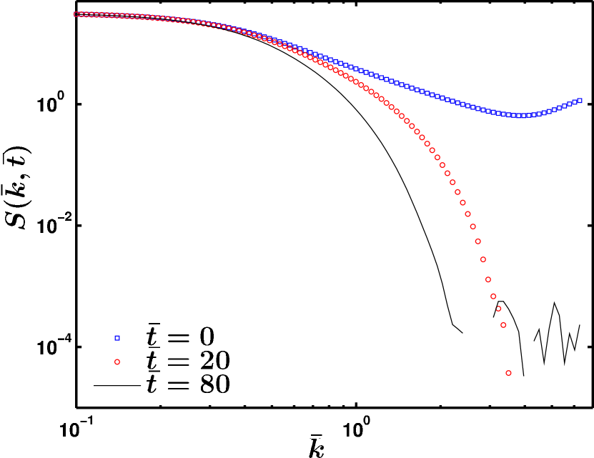
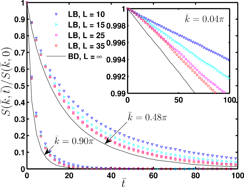
More detailed comparisons of the structure factor $S(\bar{k},\bar{t})$ are shown in Fig. 9 ($\bar{k}$ dependence at constant time) and Fig. 10 (time dependence for the normalized structure factor $S(\bar{k},\bar{t})/S(\bar{k},0)$ at constant $\bar{k}$).

Figure 9 shows the structure factor for BD simulations for a wide range of $\bar{k}$ at three different times and the data clearly indicate that the structure factor decays rapidly with time. The normalized structure factor $S(\bar{k},\bar{t})/S(\bar{k},0)$ for three different $\bar{k}$ values are shown in Fig. 10, and the data seem to indicate that the LB results approach the BD data as $L$ is increased, as expected.

III.3 Efficiency

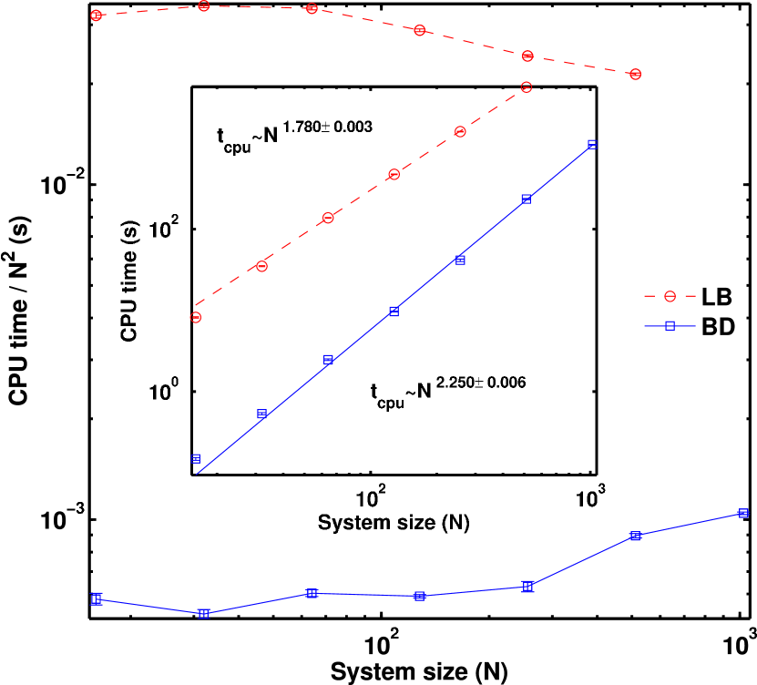
For the ultra-dilute system considered here, the lattice Boltzmann part of the hybrid LB method uses up most of the computational resources as the CPU cost for the MD part for the polymer chain is negligible. Since the dynamic properties predicted by the LB model are subject to a finite-size correction of order $L^{-1}$, extrapolation is required to obtain these properties in the asymptotic limit $L\rightarrow\infty$. To perform this extrapolation, together with checking that indeed the asymptotic $L^{-1}$ behavior has been reached, one needs the results of at least three different box lengths. Moreover, the box length should be large enough compared to the chain size such that it does not alter the static properties. The data displayed in Table 1 indicate that it is safe to choose $L$ such that $\sqrt{\left<R^{2}_{\text{e}}\right>}/L\leq 0.5$. The three different box lengths $L$ chosen here are $\sqrt{\left<R^{2}_{\text{e}}\right>}/L=0.5,0.4$, and $0.3$. In this work, we set the total CPU time required for the LB simulations to be the sum of all the CPU times required to run 1000 MD time steps for each of the chosen box lengths. For BD, we take the CPU time needed to observe the system for the same time span in physical units. Each of the simulations performed for the CPU time comparison was run on an Itanium 2 processor of a 1.6 GHz SGI Altix server 3700. All the parameters used to carry out this comparison are the optimal values for both methods. Several chain sizes ranging from $N=16$ to $1024$ have been used to obtain the CPU cost for comparison. The results are shown in Fig. 11. For the LB method, it is clear that the CPU cost scales linearly with the number of particles, i. e. the number of grid points that the solvent lives on, or $L^{3}$. Since the ratio $\sqrt{\left<R^{2}_{\text{e}}\right>}/L$ is kept constant, or $L\propto\sqrt{\left<R^{2}_{\text{e}}\right>}\propto N^{\nu}$, this leads to a CPU cost scaling as $N^{3\nu}$. This is indeed found in our benchmarks, see Fig. 11. Similarly, our data also confirm the predicted $N^{2.25}$ CPU cost scaling for BD. Though the LB exponent is lower than BD, the large prefactor ensures that the total CPU cost for LB is much more expensive compared to BD for the typical chain lengths used in the literature. It is only when the chain length is excessively large (i. e. $N$ of the order of $10^{6}$ or higher) that LB will become superior to BD for a single-chain system.

The situation completely changes if one studies a semi-dilute solution instead, as has been done in Ref. ahlrichs:01 . For such a system, we have not done a comparison between LB and BD in terms of actual simulations; however, by means of scaling considerations one can roughly estimate what the likely result of such a comparison would be. A semidilute solution comprises $M$ chains of $N$ monomers each, such that the total number of monomers is $MN$. Therefore the BD CPU cost scales as $(MN)^{2.25}$, while the LB CPU cost depends on the density. Within the blob picture of semidilute solutions, one views a chain as a sequence of “blobs”, each comprising $n$ monomers, and having size $\xi$, which can be viewed as the typical correlation length of density fluctuations, or the typical distance from which point on chain-chain interactions become important. Since the conformation statistics within the blob is that of a self-avoiding walk, one has $\xi\sim an^{\nu}$, where $a$ is the monomer size. The sequence of blobs forms a random walk, hence $R_{e}\sim\xi(N/n)^{1/2}$. This gives the minimum size of the simulation box, i. e. $L\sim\xi(N/n)^{1/2}\sim an^{\nu}(N/n)^{1/2}=aN^{\nu}(n/N)^{\nu-1/2}$, or $L^{3}\sim a^{3}N^{3\nu}(n/N)^{3\nu-3/2}$. We thus see that the CPU effort for the LB method is even slightly decreased by the factor $(n/N)^{3\nu-3/2}$ compared to the single-chain case at the same $N$, due to the shrinkage of the chains resulting from excluded-volume screening. In order to estimate the number of chains $M$, we note that the arrangement of blobs is space-filling, i. e. $L^{3}\sim\xi^{3}M(N/n)\sim a^{3}Mn^{3\nu}(N/n)$. Comparing this with the previous expression for $L^{3}$, one finds $M\sim(N/n)^{1/2}$. Therefore the BD effort, compared to the single-chain case, is increased by a factor of $M^{2.25}\sim(N/n)^{1.125}$. Taken together, this means that the ratio between LB effort and BD effort is changed by a factor of $\sim(N/n)^{3\nu+1.125-1.5}\approx(N/n)^{1.425}$ in favor of LB. For $N/n=30$, which is needed as a minimum to resolve the Gaussian statistics of the chains as a whole, one obtains a factor of $130$, which more or less compensates the two orders of magnitude seen in Fig. 11. Taking into account that for such a system the BD simulation would have to calculate the HI with the periodic images, e. g., via Ewald sums, which is much more complicated than the present single-chain simulation, one sees that for a semidilute solution clearly LB is more efficient, unless a “superfast” BD algorithm BanchioBrady03 ; Saintillanetal05 ; Hernandez-Ortizetal07 is used. For the latter case, the answer is not yet known. The results of Ref. Chenetal07 indicate that LB/MD may be favorable for a rather small number of monomers; however, this study was done (i) in a non-trivial geometry, which implies a more complicated BD method, and (ii) under complete neglect of thermal fluctuations in the LB simulations, resulting in a substantial reduction in CPU effort. Such a (partial or complete) neglect of thermal noise is sometimes justified in strong nonequilibrium situations such as studied in Ref. Chenetal07 ; in that particular case, the justification was checked by additional tests ChenPC . Another possible situation where LB noise is negligible is the case of strong coarse-graining, where a single lattice site can already be considered as a macroscopic thermodynamic system (for a detailed discussion, see Ref. DuenwegLadd09 ). However, in the general case, and certainly in thermal equilibrium or weak nonequilibrium, the proper inclusion of thermal noise is necessary, as demonstrated theoretically in detail in Ref. DuenwegLadd09 , and also corroborated by the present numerical results. For the general case, the estimate of the LB CPU effort given in Ref. Chenetal07 is therefore too optimistic.

IV Conclusions

The present study has shown that Brownian dynamics simulations are capable of reproducing various properties predicted by a hybrid LB/MD model (or vice versa). We have demonstrated how to obtain the input values for the BD simulations from the physical input parameters of the LB model such that both models would produce the same static and dynamic properties. For the LB model, most dynamic properties are subject to a finite-size correction of order $L^{-1}$. In addition to this, it is very important to thermalize all the kinetic modes in order to obtain the correct dynamic properties. Those results that are not affected by $L^{-1}$ finite size effects, such as the mean square displacement in the center of mass system, or the Rouse mode autocorrelation function, agree very favorably with each other. For highly dilute systems where the simulation of a single chain is sufficient, BD is usually the method of choice, as it is much more efficient than the coupled LB/MD approach, and finite box size effects are absent. The situation changes however in the semidilute case, where it is easy to estimate that BD will not be able to compete, unless “superfast” algorithms are used. Moreover, one should take into account that the hybrid LB/MD algorithm is rather easily adaptable to complicated boundary conditions, and can even be applied to flows at high Reynolds numbers, where the fluid degrees of freedom become intrinsically important, and cannot be handled in terms of a Green’s function.

	LB			BD
Box length $L$	10	15	25	$\infty$
Time step	0.02	0.02	0.02	0.005
exponent $\nu$	0.615 $\pm$   0.005	0.617 $\pm$ 0.005	0.619 $\pm$ 0.005	0.619 $\pm$ 0.004
$\left<\bar{R}^{2}_{\text{e}}\right>$	94.56 $\pm$ 1.20	100.05 $\pm$ 1.26	100.20 $\pm$ 1.28	99.22 $\pm$ 1.24
$\left<\bar{R}^{2}_{\text{g}}\right>$	14.83 $\pm$ 0.10	15.31 $\pm$ 0.11	15.36 $\pm$ 0.11	15.25 $\pm$ 0.11
$\left<\bar{R}_{\text{H}}^{-1}\right>_{\infty}$	0.291 $\pm$ 0.0005	0.290 $\pm$ 0.0005	0.289 $\pm$ 0.0005	0.290 $\pm$ 0.0005
$\bar{g}_{1}\text{-exp.}^{\text{a}}$	0.640 $\pm$ 0.0005	0.675 $\pm$ 0.0005	0.710 $\pm$ 0.0005	0.728 $\pm$ 0.0006
$\bar{g}_{1}\text{-exp.}^{\text{a,b}}$	0.645 $\pm$ 0.0006	0.684 $\pm$ 0.0006	0.714 $\pm$ 0.0006	0.728 $\pm$ 0.0006
$\bar{g}_{3}\text{-exp.}^{\text{a}}$	1.008 $\pm$ 0.0008	1.020 $\pm$ 0.0008	1.050 $\pm$ 0.0008	0.995 $\pm$ 0.0008
$\bar{D}_{\text{CM}}\times 10^{-3}$	3.914	5.162	6.959	9.843
	$\pm 1\times 10^{-3}$	$\pm 1\times 10^{-3}$	$\pm 2\times 10^{-3}$	$\pm 1\times 10^{-2}$
$\bar{\tau}_{\text{tr}}(\text{estimate})$	631.36 $\pm$ 4.43	492.01 $\pm$ 3.56	368.51 $\pm$ 2.67	258.28 $\pm$ 1.87

Table 1: Properties for a single chain of length $N=32$ obtained from lattice Boltzmann simulations at various finite box lengths and Brownian dynamics simulations in infinite medium. ${}^{\text{a}}$ Exponent obtained by fitting a power law in the sub-diffusive scaling regime of the chain in Lattice Boltzmann simulations, $\bar{t}\in\left[20:80\right]$. ${}^{\text{b}}$ Exponent obtained from Lattice Boltzmann simulations without thermalization of all the kinetic modes.

Figure 1: The static structure factor for the LB simulations (at various box lengths $L$) and the BD simulations ($L=\infty$) for a wide range of dimensionless wave vectors $\bar{k}$.

Figure 2: The dimensionless mean-square displacement $\bar{g}_{3}(\bar{t})$ of the chain’s center of mass, Eq. 18.

Figure 3: The dimensionless mean-square displacement $\bar{g}_{1}(\bar{t})$ of the central monomer, Eq. 19. Values of the exponent $z$ at various box length $L$ in the sub-diffusive scaling regime are also listed in Table 1.

Figure 4: The dimensionless mean-square displacement $\bar{g}_{2}(\bar{t})$ of the central monomer in the chain’s center of mass system, Eq. III.2.

Figure 5: The dimensionless long time diffusion constant for the center of mass at various box lengths $L$.

Figure 6: Normalized autocorrelation function of the first 5 Rouse modes $\mathbf{X}_{p}$ (Eq. 23) for LB simulations at $L=25$ and BD simulations at $L\rightarrow\infty$.

Figure 7: The autocorrelation function for the first Rouse mode $\mathbf{X}_{1}$ at a finite time value of $\bar{t}=700$ for LB simulations at various box lengths $L$ and BD simulations at $L\rightarrow\infty$.

Figure 8: Scaling plot of the dynamic structure factor for (a) Rouse scaling ($z=3.7$, top), (b) asymptotic Zimm scaling ($z=3$, center), and (c) $z=2.75$ (bottom), which produces the best collapse.

Figure 9: The dynamic structure factor $\bar{S}(\bar{k},\bar{t})$ for the BD simulations ($L=\infty$) at three different times.

Figure 10: Time evolution of the normalized dynamic structure factor at three different $\bar{k}$ values. Data for $\bar{k}=0.04\pi$ are displayed in the inset.

Figure 11: Comparison of the CPU time required by the LB and BD systems for the equivalent of 1000 time steps for a wide range of system sizes (chain lengths) $N$.