The $M$–$\sigma$ and $M$–$L$ Relations in Galactic Bulges, and Determinations of their Intrinsic Scatter

Abstract

We derive improved versions of the relations between supermassive black hole mass ($M_{\mathrm{BH}}$) and host-galaxy bulge velocity dispersion ($\sigma$) and luminosity ($L$) (the $M$–$\sigma$ and $M$–$L$ relations), based on 49 $M_{\mathrm{BH}}$ measurements and 19 upper limits. Particular attention is paid to recovery of the intrinsic scatter ($\epsilon_{0}$) in both relations. We find $\log(M_{\mathrm{BH}}/{\rm M}_{\scriptscriptstyle\odot})=\alpha+\beta\log(\sigma/200~{}~{}\mathrm{km~{}s^{-1}})$ with ($\alpha$, $\beta$, $\epsilon_{0}$) = ($8.12\pm 0.08$, $4.24\pm 0.41$, $0.44\pm 0.06$) for all galaxies and ($\alpha$, $\beta$, $\epsilon_{0}$) = ($8.23\pm 0.08$, $3.96\pm 0.42$, $0.31\pm 0.06$) for ellipticals. The results for ellipticals are consistent with previous studies, but the intrinsic scatter recovered for spirals is significantly larger. The scatter inferred reinforces the need for its consideration when calculating local black hole mass function based on the $M$–$\sigma$ relation, and further implies that there may be substantial selection bias in studies of the evolution of the $M$–$\sigma$ relation. We estimate the $M$–$L$ relationship as $\log(M_{\mathrm{BH}}/{\rm M}_{\scriptscriptstyle\odot})=\alpha+\beta\log(L_{V}/10^{11}{\rm L}_{{\scriptscriptstyle\odot},V})$ of ($\alpha$, $\beta$, $\epsilon_{0}$) = ($8.95\pm 0.11$, $1.11\pm 0.18$, $0.38\pm 0.09$); using only early-type galaxies. These results appear to be insensitive to a wide range of assumptions about the measurement errors and the distribution of intrinsic scatter. We show that culling the sample according to the resolution of the black hole’s sphere of influence biases the relations to larger mean masses, larger slopes, and incorrect intrinsic residuals.

1. Introduction to Black Hole Mass Relations

Studies of elliptical galaxies and spiral bulges (“hot” galaxies) have led to the discovery that most such galaxies contain massive dark objects at their centers, presumably black holes (BHs; Kormendy & Richstone, 1995; Richstone et al., 1998; Kormendy & Gebhardt, 2001). Moreover there is a remarkably tight correlation between the BH mass and the slit-averaged velocity dispersion of the hot component of the galaxy (Ferrarese & Merritt, 2000; Gebhardt et al., 2000a). This $M$–$\sigma$ relation suggests a strong link between BH formation, galaxy formation, and active galactic nuclei (AGNs).

The slope of the $M$–$\sigma$ relation has been estimated several times in the last ten years: originally $3.75\pm 0.3$ (Gebhardt et al., 2000b) and $4.8\pm 0.5$ (Ferrarese & Merritt, 2000), then $4.72\pm 0.36$ (Merritt & Ferrarese, 2001b) and $4.02\pm 0.32$ (Tremaine et al., 2002), and more recently $4.86\pm 0.43$ (Ferrarese & Ford, 2005) and $3.68\pm 0.42$ (for barless galaxies; Graham, 2008). The reasons for the differences among the different measures are discussed by Tremaine et al. (2002) and Ferrarese & Ford (2005).

There is also a relation between the BH mass and the bulge or spheroid luminosity of the galaxy (e.g., Dressler, 1989; Kormendy, 1993; Magorrian et al., 1998, and the ratio of BH mass to bulge mass was found to be $2.2^{+1.6}_{-0.9}\times 10^{-3}$ by Kormendy & Richstone 1995), but the scatter in the relation is larger than in $M$–$\sigma$. No other single parameter or combination of parameters of the host galaxy has been found to predict the BH mass with less scatter than stellar velocity dispersion (Gebhardt et al., 2003, but see also Marconi & Hunt 2003, who find a comparable scatter for the relation between BH mass and host bulge mass.).

Fundamental to the understanding of the $M$–$\sigma$ relation is the measurement of the relation’s intrinsic or cosmic scatter, as distinct from scatter due to measurement errors. Indeed, the fact that there is a relation between BH mass and stellar velocity dispersion is not surprising, but the scatter is remarkably small, estimated by Tremaine et al. (2002) to be no larger than 0.25–0.3 dex. Novak et al. (2006) carried out an extensive investigation of the residuals from proposed $M$–$\sigma$ relations and variants. Their work highlights the critical role of understanding measurement errors in assessing the scatter of the various relations.

The magnitude of the intrinsic scatter is extremely important for several reasons. First, the range of BH masses in galaxies of a given velocity dispersion or bulge luminosity constrains BH formation and evolution theories. For the past several years, many theories of BH formation and galaxy evolution have used the $M$–$\sigma$ relation either as a starting point for further work or as a prediction of the theory (e.g., Silk & Rees, 1998; Burkert & Silk, 2001; Adams et al., 2001, 2003); for a review, see Richstone (2004). A further test of such theories is whether they can reproduce the observed cosmic scatter in the relation. Some predictions that are testable in principle already exist; for example, Volonteri (2007) predicts that there should be an increased intrinsic scatter in low-mass galaxies because BHs are ejected by asymmetric gravitational wave emission and low-mass spheroids have lower escape velocities.

Understanding the scatter in the $M$–$\sigma$ relation is also essential for estimating the space density of the most massive BHs in the local universe. One of the most useful aspects of the $M$–$\sigma$ relation is that it allows one to estimate a galaxy’s central BH mass from the more easily measured velocity dispersion. Because of the steep decline in number density of galaxies having high velocity dispersion (Sheth et al., 2003; Bernardi et al., 2006; Lauer et al., 2007b), the majority of the extremely large BHs will reside in galaxies with moderate velocity dispersions that happen to contain BHs that are overmassive for the given velocity dispersion (Yu & Tremaine, 2002; Marconi et al., 2004; Lauer et al., 2007b). Knowing the magnitude of the intrinsic scatter is thus required to find the density of the most massive BHs. For example, the number density of BHs with $M>10^{10}~{}{\rm M}_{\scriptscriptstyle\odot}$ is $\sim 3~{}\mathrm{Gpc}^{-3}$ if the intrinsic scatter is 0.15 dex and $\sim 30~{}\mathrm{Gpc}^{-3}$ if the intrinsic scatter is 0.30 dex (Lauer et al., 2007b).

Both the magnitude of the intrinsic scatter and its distribution (e.g., normal or log-normal in mass) are also important to know for studies of the evolution of the $M$–$\sigma$ relation (e.g., Treu et al., 2004, 2007; Hopkins et al., 2006b; Peng et al., 2006; Shen et al., 2007, 2008; Vestergaard et al., 2008). Lauer et al. (2007a) showed that there is a bias when comparing BH masses derived from observations of inactive galaxies at low redshifts to BH masses from active galaxies at higher redshift. The bias arises because the sample of nearby galaxies measures the distribution of BH masses for a given host velocity dispersion or luminosity, whereas the sample from high-redshift galaxies tends to measure the distribution of the host luminosity or host velocity dispersion for a given BH mass. Lauer et al. (2007a) found that the bias in the inferred logarithmic mass scales as the square of the intrinsic scatter in logarithmic mass. In order to account for this bias correctly, not only the magnitude but also the distribution of the deviations from the $M$–$\sigma$ relation is needed.

Given the importance of the intrinsic scatter, we focus on a detailed examination of the scatter in the $M$–$\sigma$ and $M$–$L$ relations. This paper addresses the two most fundamental questions regarding the scatter: (1) What is the magnitude of the intrinsic scatter? and (2) What is the shape of the distribution of the intrinsic residuals? A central part of this paper is examination of the intrinsic scatter from galaxies lying in a narrow range of velocity dispersion. This sample of galaxies includes measurements from a companion paper (Gültekin et al., 2009) that presents BH mass measurements for five galaxies selected to fall within a narrow range of velocity dispersion ($180~{}~{}\mathrm{km~{}s^{-1}}<\sigma<220~{}~{}\mathrm{km~{}s^{-1}}$). By focusing on these galaxies and the others in this narrow range of velocity dispersion, we may study the distribution of BH masses at a given value of $\sigma$.

We also combine these new mass measurements with BH mass measurements and upper limits from the literature to provide new estimates of the parameters of the $M$–$\sigma$ and $M$–$L$ relations and their intrinsic scatter. We discuss our sample selection in § 2. Results of fits to $M$–$\sigma$ and $M$–$L$ as well as an analysis of their scatter are presented in § 3. We also demonstrate in § 4 that a bias is incurred by selecting a sample of BHs based on the resolution of the sphere of influence; this is our reason for including all reliable BH masses, regardless of resolution. The implications of our results are discussed in § 5 and summarized in § 6. The details of our likelihood method are described in Appendix A, and tests of various error distributions and subsample selections are provided in Appendix B.

2. Sample of Black Hole Masses

Our analysis of the $M$–$\sigma$ and $M$–$L$ relations uses a $M_{\mathrm{BH}}$ sample comprising the entire corpus of measurements published before 20 Nov 2008, augmented with the four new measurements (and one additional upper limit) presented by Gültekin et al. (2009). We surveyed the literature to make a list of dynamically detected central BHs, starting with the compilations of Tremaine et al. (2002), Marconi & Hunt (2003), Ferrarese & Ford (2005), and Graham (2008). We include only direct dynamical measurements, and since reverberation-mapping measurements (e.g., Peterson et al., 2004) are normalized to the $M$–$\sigma$ relation (Onken et al., 2004), they are not included here. Tables The $M$–$\sigma$ and $M$–$L$ Relations in Galactic Bulges, and Determinations of their Intrinsic Scatter, The $M$–$\sigma$ and $M$–$L$ Relations in Galactic Bulges, and Determinations of their Intrinsic Scatter, and The $M$–$\sigma$ and $M$–$L$ Relations in Galactic Bulges, and Determinations of their Intrinsic Scatter list all galaxies with dynamical BH measurements, with masses scaled from the original publications to our preferred distances (also listed) assuming $M_{\mathrm{BH}}\propto D$ and $H_{0}=70~{}\mathrm{km~{}s^{-1}Mpc^{-1}}$. We also include upper limits to BH masses, listed in Table The $M$–$\sigma$ and $M$–$L$ Relations in Galactic Bulges, and Determinations of their Intrinsic Scatter. Most upper limits are not restrictive, in the sense that they are consistent with a wide range of values for $M$–$\sigma$ intercept, slope and intrinsic scatter. Our fits only use BH masses from elliptical galaxies or from galaxies with classical bulges or pseudobulges (Kormendy & Kennicutt, 2004). Masses from some previous papers by our “Nuker team” (Gebhardt et al., 2000c, 2003) were 9% smaller than the correct values used here due to an error in units conversion. To correct this, the published values of $M_{\mathrm{BH}}$, $M_{\mathrm{low}}$, and $M_{\mathrm{high}}$ should be multiplied by 1.099. This correction is small compared to the measurement uncertainties, and it is indicated in Table The $M$–$\sigma$ and $M$–$L$ Relations in Galactic Bulges, and Determinations of their Intrinsic Scatter by a superscript beside the galaxies to which it has been applied.

It has been argued (e.g., Ferrarese & Ford, 2005) that BH mass determinations are unreliable if the kinematic observations do not resolve the sphere of influence of radius $R_{\mathrm{infl}}=GM_{\mathrm{BH}}\sigma^{-2}$. In particular the argument generally requires that the full width at half-maximum intensity (FWHM) spatial resolution of the kinematic observations, $d_{\mathrm{res}}$, satisfy $R_{\mathrm{infl}}/d_{\mathrm{res}}>1$ to avoid bias in the BH mass determination. We do not agree with this argument: our tests (Gebhardt et al., 2003; Kormendy, 2004) show that the smaller values of $R_{\mathrm{infl}}/d_{\mathrm{res}}$ lead to large error bars but not systematic bias. We expand on the misconception that under-resolved spheres of influence lead to biased BH mass determinations in § 4.1. On the other hand, we show in § 4 that excluding measurements on the basis of $R_{\mathrm{infl}}/d_{\mathrm{res}}$ leads to systematic bias, not in the individual BH masses, but in the estimates of the parameters of the $M$–$\sigma$ and $M$–$L$ relations. For these reasons we do not adopt any resolution-based cutoff in measurements included in our sample. We also investigate each BH mass detection individually and decide whether any systematic uncertainties suggest that it should be omitted from our sample. In Table The $M$–$\sigma$ and $M$–$L$ Relations in Galactic Bulges, and Determinations of their Intrinsic Scatter we list published BH masses that we omit from our fitting sample as well as the reasons. In general, galaxies are omitted because (1) the authors of the study, themselves, expressed doubts of their models’ ability to securely determine the mass, (2) there is no quantitative analysis of how well their model fits the data (e.g., the value of reduced $\chi^{2}$ for the best fit), or (3) the provided quantitative analysis of goodness of fit is poor. Note that one of the major conclusions of this paper is that the intrinsic scatter of the $M$–$\sigma$ relation is larger than most previous studies have been found. If we did not omit the galaxies in Table The $M$–$\sigma$ and $M$–$L$ Relations in Galactic Bulges, and Determinations of their Intrinsic Scatter, the scatter would increase further. After removing these BH masses, we are left with a sample including upper limits (SU, see Table 2 for abbreviations used to denote our samples) and a sample excluding upper limits (S).

In Appendix B we also consider an additional sample. Following the suggestion of Ferrarese & Ford (2005) and others, we create a “restricted sample” (RS) of only 20 galaxies in which we (1) require $R_{\mathrm{infl}}/d_{\mathrm{res}}\geq 1.0$, (2) use only detected BH masses (i.e., no upper limits), (3) exclude masses deemed suspicious by Ferrarese & Ford (2005) or by Tremaine et al. (2002) in their final “culled sample,” (4) exclude any galaxy in which multiple measurements are inconsistent, and (5) make a subjective judgment that the quality of the mass determination is adequate. Because of the bias introduced by restrictions based on resolution, we do not recommend this approach, but we present fits to Sample RS in Appendix B.

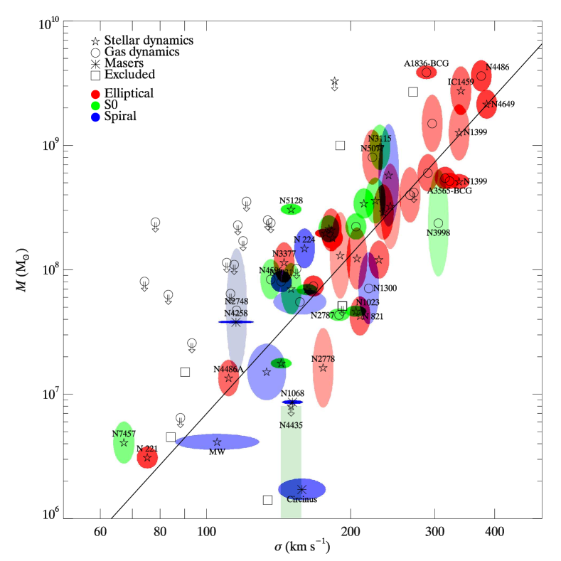
Membership in all samples (SU, S, RS) is given in Tables The $M$–$\sigma$ and $M$–$L$ Relations in Galactic Bulges, and Determinations of their Intrinsic Scatter and The $M$–$\sigma$ and $M$–$L$ Relations in Galactic Bulges, and Determinations of their Intrinsic Scatter. We plot the masses of the BHs as a function of velocity dispersion in Figure 1.

Figure 1.— The $M$–$\sigma$ relation for galaxies with dynamical measurements. The symbol indicates the method of BH mass measurement: stellar dynamical (pentagrams), gas dynamical (circles), masers (asterisks). Arrows indicate 3$\sigma_{68}$ upper limits to BH mass. If the 3$\sigma_{68}$ limit is not available, we plot it at 3 times the 1$\sigma_{68}$ or at 1.5 times the 2$\sigma_{68}$ limits. For clarity, we only plot error boxes for upper limits that are close to or below the best-fit relation. The color of the error ellipse indicates the Hubble type of the host galaxy: elliptical (red), S0 (green), and spiral (blue). The saturation of the colors in the error ellipses or boxes is inversely proportional to the area of the ellipse or box. Squares are galaxies that we do not include in our fit. The line is the best fit relation to the full sample: $M_{\mathrm{BH}}=10^{8.12}~{}{\rm M}_{\scriptscriptstyle\odot}(\sigma/200~{}~{}\mathrm{km~{}s^{-1}})^{4.24}$. The mass uncertainty for NGC 4258 has been plotted much larger than its actual value so that it will show on this plot. For clarity, we omit labels of some galaxies in crowded regions.

2.1. Velocity Dispersion

Whenever possible we use the effective velocity dispersion $\sigma_{e}$ as defined by

$$\sigma^{2}_{e}\equiv\frac{\int_{0}^{R_{e}}\left({\sigma^{2}+V^{2}}\right)I\left(r\right)dr}{{\int_{0}^{R_{e}}I\left(r\right)dr}},$$ (1)

where $R_{e}$ is the effective radius of the galaxy and $V$ is the rotational component of the spheroid. If this is not available, we use the central stellar velocity dispersion ($\sigma_{c}$) found in HyperLeda. In galaxies for which both are available, we compare $\sigma_{e}$ to $\sigma_{c}$ in Figure 2 and find no systematic bias to high or low values. Because of stellar template mismatches and possible errors in the determination of $R_{e}$, we impose a minimum error in $\sigma_{e}$ of 5%. The contribution to velocity dispersion arising from the relatively small rotational component of disks in spiral galaxies is unlikely to lead to large systematic errors in velocity dispersion. For this reason, we include spirals in our main sample.

Figure 2.— Central stellar velocity dispersion $\sigma_{c}$ from HyperLEDA as a function of effective stellar velocity dispersion $\sigma_{e}$ (eq. 1). There is no systematic bias to high or low values. The dotted line shows $\sigma_{c}=\sigma_{e}$. The solid line is the best-fit regression, $\sigma_{c}=(-2.7\pm 1.4~{}~{}\mathrm{km~{}s^{-1}})+(1.00\pm 0.02)\sigma_{e}$. The dashed line is a fit that includes uncertainties in both variables as well as an intrinsic scatter: $\sigma_{c}=(-0.9\pm 7.2~{}~{}\mathrm{km~{}s^{-1}})+(0.95\pm 0.09)\sigma_{e}$ with intrinsic scatter of $22\pm 5~{}~{}\mathrm{km~{}s^{-1}}$. Both fits are consistent with $\sigma_{c}=\sigma_{e}$ within their uncertainties.

2.2. Luminosities

We use extinction-corrected, bulge (which we obviously interpret as total luminosity for ellipticals), $V$-band luminosities–calculated from the extinction-corrected magnitudes, $M_{V,{\mathrm{bulge}}}^{0}$, using $\log(L_{V}/{\rm L}_{{\scriptscriptstyle\odot},V})=0.4(4.83-M_{V,{\mathrm{bulge}}}^{0})$. The choice of $V$ band is a compromise between more widely available luminosities in the $B$ and $V$ bands and less extinguished $K$-band luminosities. Because bulge-disk decomposition of spiral galaxies is fraught with difficulties and possible systematic errors, we do not include spirals in the $M_{\rm BH}$–$L$ fits. We do include bulge luminosities for S0 galaxies for which we are confident in the bulge-disk decomposition because the disk is faint and contains little dust and few young stars. Errors in bulge-disk decomposition were estimated by examining the range of values in the literature. Thus the galaxies included in $M$–$L$ fits are those which have a $M_{V,{\mathrm{bulge}}}^{0}$ value listed in Table The $M$–$\sigma$ and $M$–$L$ Relations in Galactic Bulges, and Determinations of their Intrinsic Scatter or The $M$–$\sigma$ and $M$–$L$ Relations in Galactic Bulges, and Determinations of their Intrinsic Scatter. Most of our $V$-band absolute magnitudes (total and bulge) come directly from de Vaucouleurs et al. (1991) as compiled by Lauer et al. (2005) and Lauer et al. (2007c).

3. Measurement of the $M$–$\sigma$ and $M$–$L$ Relations, and their Intrinsic Scatter

3.1. Best Fit $M$-$\sigma$ Relation

We are principally interested in predictors of the form

$$\log{(M/{\rm M}_{\scriptscriptstyle\odot})}=\alpha+\beta\log{\left(\sigma_{e}/200~{}\mathrm{km~{}s^{-1}}\right)},$$ (2)

with an intrinsic or cosmic scatter $\epsilon_{0}$ that is the root-mean square (rms) deviation in $\log(M_{\mathrm{BH}}/{\rm M}_{\scriptscriptstyle\odot})$ from this relation (for zero measurement error). We assume for simplicity that $\epsilon_{0}$ is independent of $\sigma_{e}$. The details of the fitting method are discussed in Appendix A. Based on tests in § 3.2, a log-normal distribution of intrinsic scatter $\epsilon_{0}$ is an adequate description of the scatter. Based on tests in Appendix B, a generalized maximum-likelihood method is appropriate to use here. Given these, the best-fit relation for the full sample (SU) is

$$\log{\left(\frac{M}{{\rm M}_{\scriptscriptstyle\odot}}\right)}=(8.12\pm 0.08)+(4.24\pm 0.41)\log{\left(\frac{\sigma_{e}}{200~{}\mathrm{km~{}s^{-1}}}\right)},$$ (3)

which has an intrinsic rms scatter $\epsilon_{0}=0.44\pm 0.06$. These values are very close to those obtained by Tremaine et al. (2002). We show in Appendix B that the choice of objects to include in the sample can have a significant impact on the slope, intercept, and residual scatter, but that the error distribution assumed (among those we considered) has little impact.

The full sample may be split into subsamples: early-type (elliptical and S0) and late-type (spiral) galaxies, ellipticals and non-ellipticals, BH mass measurements by gas dynamics and other methods, low $\sigma_{e}$ and high $\sigma_{e}$, and barred and non-barred galaxies. The fits are summarized in Table 1. In most cases the fits to different subsamples are consistent with each other. The intrinsic scatter for the ellipticals-only sample, however, is $\epsilon_{0}=0.31\pm 0.06$, which is $\sim$2$\sigma_{68}$ smaller than either the full sample ($\epsilon_{0}=0.44\pm 0.06$) or the sample of non-ellipticals ($\epsilon_{0}=0.53\pm 0.10$). This may reflect either greater unaccounted errors in BH mass and $\sigma_{e}$ measurements in later-type galaxies, or that ellipticals lie closer to the ridge line of the $M$–$\sigma$ relation than later-type galaxies.

Table 1$M$–$\sigma$ Relation for Subsamples

Subsample	$N_{m}$	$N_{u}$	$\alpha$	$\beta$	$\epsilon_{0}$	$P_{\emptyset}$
Full sample	49	18	$8.12\pm 0.08$	$4.24\pm 0.41$	$0.44\pm 0.06$	$0.0004\pm 0.018$
Early type	38	6	$8.22\pm 0.073$	$3.86\pm 0.380$	$0.35\pm 0.031$	$0.0145\pm 0.031$
Late type	11	12	$7.95\pm 0.286$	$4.58\pm 1.583$	$0.56\pm 0.141$	$0.0006\pm 0.040$
Ellipticals	25	2	$8.23\pm 0.084$	$3.96\pm 0.421$	$0.31\pm 0.063$	$0.0006\pm 0.018$
Non-ellipticals	24	16	$8.01\pm 0.156$	$4.05\pm 0.831$	$0.53\pm 0.097$	$0.0010\pm 0.031$
Stars and masers	32	2	$8.11\pm 0.107$	$4.05\pm 0.554$	$0.49\pm 0.075$	$0.0002\pm 0.021$
Gas dynamics	17	16	$8.16\pm 0.122$	$4.58\pm 0.652$	$0.35\pm 0.096$	$0.0036\pm 0.040$
$\sigma_{e}<200~{}~{}\mathrm{km~{}s^{-1}}$	25	16	$8.07\pm 0.172$	$3.97\pm 0.869$	$0.50\pm 0.091$	$0.0013\pm 0.031$
$\sigma_{e}>200~{}~{}\mathrm{km~{}s^{-1}}$	24	2	$8.12\pm 0.158$	$4.47\pm 0.921$	$0.35\pm 0.079$	$0.0026\pm 0.024$
Non-barred	41	7	$8.19\pm 0.087$	$4.21\pm 0.446$	$0.43\pm 0.064$	$0.0006\pm 0.017$
Barred	8	11	$7.67\pm 0.115$	$1.08\pm 0.751$	$0.17\pm 0.078$	$0.1809\pm 0.147$
Classical bulges	39	16	$8.17\pm 0.086$	$4.13\pm 0.434$	$0.45\pm 0.066$	$0.0009\pm 0.024$
Pseudobulges	10	2	$7.98\pm 0.156$	$4.49\pm 0.903$	$0.28\pm 0.096$	$0.0034\pm 0.037$

Note. — Results from fits to subsamples of our full sample, based on morphological type, BH mass-measurement method. $N_{m}$ and $N_{u}$ are the number of galaxies in each group with BH mass measurements and upper limits, respectively.

3.2. Examination of the Intrinsic Scatter in $M$–$\sigma$

The distribution of residuals from the $M$–$\sigma$ relation is of practical interest as discussed in § 1. Figure 3 is a histogram of the residuals in $\log{(M_{\mathrm{BH}})}$ in the best-fit $M$–$\sigma$ relation from sample S. The distribution of the residuals appears consistent with a normal or Gaussian distribution in logarithmic mass, although the distribution is noisy because of the small numbers. For a more direct test of normality we look at $\log(M_{\mathrm{BH}})$ in galaxies with $\sigma_{e}$ between $165$ and $235~{}\mathrm{km~{}s^{-1}}$, corresponding to a range in $\log(\sigma_{e}/200~{}\mathrm{km~{}s^{-1}})$ from approximately $-0.075$ to $0.075$. The predicted masses for the 19 galaxies in this narrow range differ by at most a factor of 4.3, given our best-fit relation. The power of having a large number of galaxies in a narrow range in velocity dispersion is evident here, as there is no need to assume a value for the slope of $M$–$\sigma$ or even that a power-law form is the right model. The only assumption required is that the ridge line of any $M$–$\sigma$ relation that may exist does not change substantially across the range of velocity dispersion. The mean of the logarithmic mass in solar units is 8.16, and the standard deviation is 0.45. The expected standard deviation in mass is 0.19, based on the rms dispersion of $\log(\sigma_{e}/200~{}\mathrm{km~{}s^{-1}})$ (0.046) in this range times the $M$–$\sigma$ slope $\beta$; thus the variation in the ridge line of the $M$–$\sigma$ relation in this sample is negligible compared to the intrinsic scatter. We perform an Anderson-Darling test for normality with unknown center and variance on this sample of logarithmic masses (Stephens, 1974; Press et al., 1986) and find that the distribution is consistent with normality at better than the 15% level. The same sample fails an Anderson-Darling test for normality in $M_{\mathrm{BH}}$ — as opposed to $\log(M_{\mathrm{BH}})$ — at the 1% level.

Figure 3.— Histogram of residuals from the best-fit $M$–$\sigma$ relation in sample S.

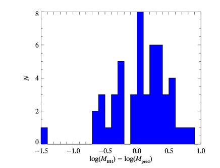
The Anderson-Darling tests show that log-normal (i.e., Gaussian in logarithmic mass) is an acceptable description of the distribution of the residuals. The residuals may also be well represented by other distributions, which may be compared to a log-normal description with an odds ratio (Eq. A18). The calculated odds ratio of Gaussian to Lorentzian in logarithmic mass is 14.49, of Gaussian to double-sided exponential in logarithmic mass is 1.78, of Gaussian to the sum of two Gaussians in logarithmic mass is 1.55, and of Gaussian to a Gaussian with different standard deviations above and below the mean is 2.30. In these cases considered, the odds ratio (${\mathcal{R}}_{ab}$) of the Gaussian distribution to the other distributions in logarithmic mass is greater than unity. Thus the Gaussian distribution is favored. While it should be noted that these tests convolve the intrinsic dispersion with variance from imprecise measurements, the residuals in the $M$–$\sigma$ relation are well described by a Gaussian distribution in logarithmic mass.

One component of the intrinsic scatter in both the $M$–$\sigma$ and $M$–$L$ relations is sure to be random errors in distance.

All BH mass measurements in our sample scale other than the Milky Way linearly with the distance. For these galaxies random errors in distance contribute directly to uncertainty in the mass and thus contributes to the intrinsic scatter. The Milky Way, which scales approximately as $D^{1.8}$ (Ghez et al., 2008), has the uncertainty in distance incorporated in its mass uncertainty in our tables. The contribution of random errors in distance to the intrinsic scatter, however, is sure to be a small as the random errors in distance are typically around 10% or 0.04 dex (e.g., Tonry et al., 2001) compared to the scatter of $0.44$ dex. Another source of intrinsic scatter may be unaccounted systematic errors in $M_{\mathrm{BH}}$ measurements. In this paper, we assume that the measurement errors accurately reflect the uncertainty, but we discuss some possible cuases in § 5.1. If systematics are large, then they may be an important contribution to the inferred intrinsic scatter.

3.3. Log-Quadratic Fits to $M$–$\sigma$

We may also fit a log-quadratic function to the data as suggested by Wyithe (2006a):

$$\log{\left(\frac{M_{\mathrm{BH}}}{{\rm M}_{\scriptscriptstyle\odot}}\right)}=\alpha + \beta\log{\left(\frac{\sigma_{e}}{200~{}\mathrm{km~{}s^{-1}}}\right)}$$ (4)

$$+ \gamma\left[\log{\left(\frac{\sigma_{e}}{200~{}\mathrm{km~{}s^{-1}}}\right)}\right]^{2}.$$

For the full sample, we find $\alpha=8.08\pm 0.10$, $\beta=4.47\pm 0.50$, $\gamma=1.72\pm 1.71$, and $\epsilon_{0}=0.44\pm 0.06$. The results are consistent with log-linear ($\gamma=0$) at the 1$\sigma_{68}$ level, and the intrinsic scatter is not significantly decreased from a log-linear model. The value and significance for $\gamma$ is similar to that found by Wyithe (2006b). The odds ratio (eq. A18) of a log-linear model to a log-quadratic model is ${\mathcal{R}}_{ab}=4.68$, indicating the log-linear model is favored.

3.4. Best-Fit $M$–$L$ Relation

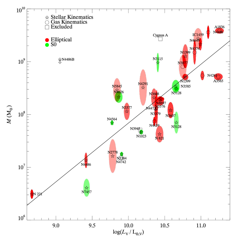
We also look at fits to the $M$–$L$ relation. Spiral galaxies, which present problems in determining the bulge luminosity because of the difficulty in getting a precise bulge-disk decomposition, are excluded. We therefore limit our fits to ellipticals and those S0 galaxies for which we have reliable bulge-disk decomposition. The sample of galaxies used may be discerned from Tables The $M$–$\sigma$ and $M$–$L$ Relations in Galactic Bulges, and Determinations of their Intrinsic Scatter and The $M$–$\sigma$ and $M$–$L$ Relations in Galactic Bulges, and Determinations of their Intrinsic Scatter by the presence of a value in the column for bulge magnitude ($M^{0}_{V,\mathrm{bulge}}$), which in the case of ellipticals is equal to the total magnitude.

Using the same fitting method as before on all galaxies meeting the above criteria, we find

$$\log{\left(\frac{M}{{\rm M}_{\scriptscriptstyle\odot}}\right)}=(8.95\pm 0.11)+(1.11\pm 0.18)\log{\left(\frac{L_{V}}{10^{11}{\rm L}_{{\scriptscriptstyle\odot},V}}\right)}$$ (5)

with an intrinsic scatter of $\epsilon_{0}=0.38\pm 0.09$.

Figure 4.— The $M$–$L$ relation for galaxies with dynamical measurements. The symbol indicates the method of BH mass measurement: stellar dynamical (pentagrams) and gas dynamical (circles). Arrows indicate upper limits for BH mass. Squares are galaxies that we omitted from the fit. The color of the error ellipse indicates the Hubble type of the host galaxy [elliptical (red) and S0 (green)] and the saturation of the color is inversely proportional to the area of the ellipse. The line is the best-fit relation for the sample without upper limits: $M_{\mathrm{BH}}=10^{8.95}~{}{\rm M}_{\scriptscriptstyle\odot}(L_{V}/10^{11}~{}{\rm L}_{{\scriptscriptstyle\odot},V})^{1.11}$.

3.5. Examination of the Intrinsic Scatter in $M$–$L$

The scatter determined here for the $M$–$L$ relation is notably smaller than other studies have found, and it is consistent with the intrinsic scatter in $M$–$\sigma$ in early-type galaxies. Other studies have found similar scatter between the $M$–$L$ and $M$–$\sigma$ relations (e.g., Marconi & Hunt, 2003). Figure 5 shows a histogram of the residuals from the fit. We test the distribution of 12 masses in a narrow range in luminosity ($10.2<\log{(L_{\mathrm{V}}/{\rm L}_{{\scriptscriptstyle\odot}\mathrm{,V}})<10.7}$) for normality and log-normality using an Anderson-Darling test with unknown mean and variance. The mean logarithmic BH mass in that range is 8.21 with standard deviation 0.36. The expected standard deviation in logarithmic mass is 0.16, if all the galaxies lie exactly on the ridge line of the $M$–$L$ relation, based on standard deviation in logarithmic luminosity of 0.14. Thus the variation in the ridge line of the $M$–$L$ relation in this sample is negligible compared to the intrinsic scatter. The distribution of masses is consistent with a log-normal distribution, but is inconsistent with a normal distribution at the 1% level.

Figure 5.— Histogram of residuals from best-fit $M$–$L$ relation.

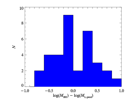
Again, we consider several possible functional forms of the intrinsic scatter in logarithmic mass at constant luminosity and calculate odds ratios of Gaussian to Lorentzian (3.37), to double-sided exponential (1.10), to double Gaussian (1.36), and to a Gaussian with different standard deviations above and below the mean (1.99). Thus, normal or double-sided exponential in logarithmic mass are equally acceptable descriptions of the intrinsic scatter. There are, however, relatively few mass measurements in this range, so this it is not as strong a test as it is for $M$–$\sigma$.

4. Biases Introduced When Culling the Sample by Black Hole Sphere-of-Influence Resolution

Our analysis has used all $M_{\mathrm{BH}}$ measurements in the sample without regard to how well the sphere of influence is resolved. In essence, we trust the uncertainties returned by the dynamical models to reflect the quality of the $M_{\mathrm{BH}}$ determination—given the assumptions—for whatever resolution was realized. This approach conflicts with the caveats advanced by, e.g., Ferrarese (2002), who concluded that $R_{\mathrm{infl}}/d_{\mathrm{res}}>1$ was a necessary (but not sufficient) condition to make a precise $M_{\mathrm{BH}}$ determination. Such concerns have motivated a number of groups studying the BH relations (e.g., Merritt & Ferrarese, 2001b; Ferrarese & Ford, 2005) to cull the more poorly resolved BHs from their samples. We show in this section that far from improving the accuracy of the estimated relations, this procedure will actually produce biased estimates of the intercept, slope, and intrinsic scatter of the relations.

4.1. What Resolution of the Sphere of Influence Does and Does Not Mean

We advocate use of the sphere-of-influence scale only as a rough guide to the needed spatial resolution of the observations. In the arguments that follow, we will show that $M_{\mathrm{BH}}$ determinations from datasets with $R_{\mathrm{infl}}/d_{\mathrm{res}}<1$ are unbiased when using three-integral models. This, however, contrasts with claims commonly made in other works: that strict resolution of the sphere of influence is required for credible $M_{\mathrm{BH}}$ determinations and more importantly, that $M_{\mathrm{BH}}$ determinations made from observations that do not resolve the sphere of influence will be biased. Given the strong prevalence of this viewpoint, and prompted by comments from the referee, we review its development and application in the literature. We find, in fact, that there is little or no support for the conclusion that $M_{\mathrm{BH}}$ determination become increasingly biased with decreasing resolution. It appears that the common but uncritical application of sphere-of-influence-resolution as a way to cull $M_{\mathrm{BH}}$ determinations cannot be justified by careful reading of the very works often cited in its support.

In their review article, Ferrarese & Ford (2005) write, “All studies which have addressed the issue [of BH mass determination and resolution level]…have concluded that resolving the sphere of influence is an important (although not sufficient) factor: not resolving [$R_{\mathrm{infl}}$] can lead to systematic errors on $M_{\mathrm{BH}}$ or even spurious detections,” and cite the following: Ferrarese & Merritt (2000); Merritt & Ferrarese (2001b, a); Graham et al. (2001); Ferrarese (2002); Marconi & Hunt (2003). We consider each of these in turn.

Ferrarese & Merritt (2000) found that the ground-based $M_{\mathrm{BH}}$ measurements by Magorrian et al. (1998) were higher for fixed velocity dispersion than the predictions of their empirical $M$–$\sigma$ relation and judged them to be therefore biased. The discrepancy with their $M$–$\sigma$ relation increased with increasing distance. While discrepancy with the $M$–$\sigma$ relation is not a justifiable reason for excluding $M_{\mathrm{BH}}$ measurements from the relation (the argument is circular), the masses from Magorrian et al. (1998) were, in fact, biased to high values by roughly a factor of 3. The reason for the bias, however, is that they came from two-integral, isotropic, axisymmetric models, not because they were more poorly resolved (Merritt & Ferrarese, 2001a; Gebhardt et al., 2003).

Merritt & Ferrarese (2001b) present similar arguments as do Merritt & Ferrarese (2001a) who also go on to describe the reason two-integral models yield masses that are biased somewhat high. Merritt & Ferrarese (2001a) do mention that three-integral models provide an increased space of orbits that can lead to an increased range in acceptable black hole masses but not that they are biased, resolved or not.

Graham et al. (2001) find decreased scatter in the relation between $M_{\mathrm{BH}}$ and concentration index when removing more poorly resolved galaxies in addition to another galaxy. Again, using a provisional relation to exclude potential data points from the relation is not the same as the identification of a bias.

Ferrarese (2002) does not present new arguments or studies but repeats the arguments just described.

Marconi & Hunt (2003) say nothing about a bias, only that they used $R_{\mathrm{infl}}/d_{\mathrm{res}}$ as a criterion for determining reliable masses and that they find a smaller scatter in the $K$-band $M$–$L$ relation when excluding lower resolution observations.

Valluri et al. (2004) are frequently cited as having shown that resolving the sphere of influence is necessary for accurate $M_{\mathrm{BH}}$ determination, but, in fact, they do not make such a claim. The most important result from their work was to show that when using too few orbits, spurious black hole mass determinations may appear. When enough orbits are used, Valluri et al. (2004) found that a wide range of values for $M_{\mathrm{BH}}$ are acceptable with their synthetic data set, but this turns out to be caused by the lack of real measurement noise in the data set (Magorrian, 2006). Even so, the input $M_{\mathrm{BH}}$ in their simulations was always within their range of acceptable values, i.e., not biased. The bias that Valluri et al. (2004) do identify is what results from over-regularizing (i.e., requiring smoothness in orbit solutions) not from under-resolving the sphere of influence.

The degree of resolution of the sphere of influence of the BH cannot tell the complete story of the reliability of the BH mass determination. In the quantity $R_{\mathrm{infl}}/d_{\mathrm{res}}$ there is encoded no information about, e.g., the spectroscopic resolution of the data. To illustrate this, we perform a simple experiment. We take surface brightness profiles, $I(r)$, from two galaxies with velocity dispersion $\sigma_{e}\approx 200~{}\mathrm{km~{}s^{-1}}$, one a core galaxy (NGC 3607) and one a power-law galaxy (NGC 4026), and deproject to get luminosity densities. We assume a constant mass-to-light ratio of $\Upsilon=4$ and calculate the projected velocity dispersion profile, $\sigma_{0}(r)$ from a spherical, isotropic model, assuming a seeing of 0$\farcs$1. We repeat this process but this time assuming there is a black hole with mass $M_{\mathrm{BH}}=10^{8}{\rm M}_{\scriptscriptstyle\odot}$ at the center to get $\sigma_{\mathrm{BH}}(r)$. We then calculate the difference in projected velocity dispersions from the two models. The ability to discriminate between these two models depends on the measurement error of velocity dispersion, $\delta_{\sigma}$. We calculate the significance of the difference between these models $[\sigma_{\mathrm{BH}}(r)-\sigma_{0}(r)]/\delta_{\sigma}$ for three values of the measurement error $\delta_{\sigma}=5$, $10$, and $20~{}\mathrm{km~{}s^{-1}}$, which roughly correspond to signal-to-noise ratios from HST STIS data of more than $50$, $40$ to $50$, and $35$, respectively, depending on the details of the observation. We plot these curves in Figure 6 as solid lines. Two conclusions are immediately obvious from these curves: (1) It is possible to discern a significant difference between the two profiles outside of $r/R_{\mathrm{infl}}=2$ (corresponding to $R_{\mathrm{infl}}/d_{\mathrm{res}}<1$), and (2) the significance of the difference depends on the measurement errors. An actual observation would amplify the difference because, rather than comparing the two velocity dispersion profiles at one location in radius, it would integrate the velocity dispersion within a resolution bin. To illustrate this we calculate $[\Sigma_{\mathrm{BH}}(r)-\Sigma_{0}(r)]/\delta_{\sigma}$, where

$$\Sigma^{2}_{\mathrm{BH}}(r)=\frac{\int_{0}^{r}\sigma^{2}_{\mathrm{BH}}(r)I(r)rdr}{\int_{0}^{r}I(r)rdr}$$ (6)

and similarly for $\Sigma_{0}$. We plot these as dashed lines in Figure 6 for each of the representative measurement errors. These curves show that it is possible to determine the presence of a BH when your data do not resolve the sphere of influence, depending on the quality of the data.

Figure 6.— Plots of significance of the difference between velocity dispersions of a galaxy with a BH and one without. The solid lines show $(\sigma_{\mathrm{BH}}-\sigma_{0})/\delta_{\sigma}$ as a function of radial distance in units of $R_{\mathrm{infl}}$ for three different values of measurement error in velocity dispersion. The dashed curves show the difference between light-weighted integrated velocity dispersion profiles. The left panel is derived from NGC 3607, a galaxy with a core surface brightness profile, and the right panel is derived from NGC 4026, a galaxy with a power-law surface brightness profile. It is clear that (1) it is possible to discern the presence of a BH outside of the sphere of influence and (2) the ability to discern the presence of a BH depends on the measurement error.

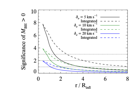
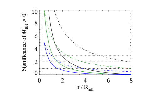
It is further evident from the figure that for a given measurement error in velocity dispersion, the ability to discriminate between different BH masses decreases further away from the center, i.e., errors in BH mass increase as $R_{\mathrm{infl}}/d_{\mathrm{res}}$ decreases. This fact has been seen several times before in the literature. Gebhardt et al. (2003) modeled 12 galaxies using (1) ground-based data only and (2) ground-based data combined with space-based data. In every case, the models recover larger uncertainties for the data sets with only ground-based data. A separate study, by Kormendy (2004), considered the many mass measurements of the BH in M32 using a variety of modeling techniques and data that range in level of resolution by over an order of magnitude. The study revealed that the error bars in the $M_{\mathrm{BH}}$ determination increased as $R_{\mathrm{infl}}/d_{\mathrm{res}}$ decreased but that the $M_{\mathrm{BH}}$ values were not biased at any resolution. In fact, the value for $M_{\mathrm{BH}}$ found from the highest resolution data was consistent with all of the lower resolution results. This held true despite the fact that the values considered were derived from widely varying modeling methods.

When looking at the data in Table The $M$–$\sigma$ and $M$–$L$ Relations in Galactic Bulges, and Determinations of their Intrinsic Scatter, it is tempting to look for a correlation between the size of the error in BH mass and $R_{\mathrm{infl}}/d_{\mathrm{res}}$, but the size of the error depends on many factors. Among the factors are differences in method of BH mass determination, differences in codes within similar methods, and varying quality data among the different galaxies. When considering only stellar dynamical mass determinations by the code described by Siopis et al. (2008), there is a weak yet significant trend, as seen in Figure 7, which plots $M_{\mathrm{high}}/M_{\mathrm{low}}$ as a function of $R_{\mathrm{infl}}/d_{\mathrm{res}}$. This trend is weak because of other factors that determine the precision of the measurement.

Figure 7.— Plot of size of errors in BH mass, calculated as $M_{\mathrm{high}}/M_{\mathrm{low}}$, as a function of $R_{\mathrm{infl}}/d_{\mathrm{res}}$ for stellar dynamical measurements using the code described in Siopis et al. (2008). There is a weak but significant trend indicating that lower resolution contributes to larger errors in BH mass, but it is not the only factor in determining the uncertainty.

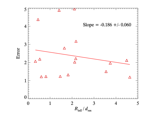
We stress again that larger error bars do not imply a bias in the value of BH mass recovered from observations with smaller $R_{\mathrm{infl}}/d_{\mathrm{res}}$. For example, Gebhardt et al. (2003) show that there is no significant bias in their figure 9, which plots BH masses obtaimed from ground-based data alone as a function of masses from the same ground-based data combined with space-based data. The line of equality in their figure goes through 10 of the 12 error bars. In 4 of the 12 galaxies, the difference between the best-fit values is less than 25%, and in 9 of the 12 it is less than 50%. While 9 of the 12 have smaller values of $M_{\mathrm{BH}}$ for ground-only datasets (actually the opposite bias to that seen in the Magorrian et al. (1998) models, which is additional evidence that the limited resolution does not produce a systematic bias), for 12 independent trials of an event with 50% chance of success, there will be 9 or more successes 7.3% of the time. This is entirely consistent with no bias. So while increased spatial resolution will always improve the precision of BH measurements, this trend appears to be correctly reflected in the larger error bars that emerge from the modeling procedure.

4.2. Simulated Sample of Galaxies

We demonstrate the effects of such a culled sample selection with a series of simple Monte Carlo experiments on a synthetic $M$–$\sigma$ data set. Each synthetic data set consists of a sample of 40 galaxies, uniformly distributed in volume out to a distance of 30 Mpc. Each galaxy is given a velocity dispersion from a normal distribution in $\log{(\sigma/200~{}~{}\mathrm{km~{}s^{-1}})}$ centered at 0 with standard deviation 0.2. Each galaxy is given a BH mass from an $M$–$\sigma$ relation with $\alpha=8$, $\beta=4.0$, and log-normal intrinsic scatter with $\epsilon_{0}=0.3$ dex. The BH’s logarithmic mass is measured with a normally distributed measurement error of 0.2 dex and the velocity dispersion has a 5% error. Since each galaxy has a distance, a BH mass, and a velocity dispersion, we calculate $R_{\mathrm{infl}}=GM_{\mathrm{BH}}\sigma^{-2}$ and assume the galaxy to be observed with an instrument with resolution of $d_{\mathrm{res}}=0\farcs 1$. This process is repeated for $10^{5}$ realizations for each of the choices in assembling the sample described below.

We first tried fitting for the parameters of the $M$–$\sigma$ relation using these simulated data sets and the same fitting procedures that we applied earlier to the actual data. We successfully recovered the input parameters with only a slight bias to low intrinsic scatter (recovering $\epsilon=0.27$ instead of the input value of $0.3~{}\mathrm{dex}$). The samples were then culled in two ways: (1) we removed galaxies that fell below a given cutoff in $R_{\mathrm{infl}}/d_{\mathrm{res}}$, where $R_{\mathrm{infl}}$ is computed from the measured BH mass and velocity dispersion; and (2) we removed galaxies that fell below a given cutoff in $R_{\mathrm{infl}}/d_{\mathrm{res}}$, where $R_{\mathrm{infl}}$ is computed from the BH mass predicted by the $M$–$\sigma$ relation. Since the Galaxy plays an important role in the observed sample (because of its position near the low end of the range of observed $\sigma_{e}$ and the small uncertainty in the measured mass), we also augmented some of the samples by adding one galaxy with the actual measured values of the Galaxy’s BH mass and velocity dispersion with their corresponding uncertainties.

4.3. Culling the Simulated Sample Based on Traditional Sphere of Influence

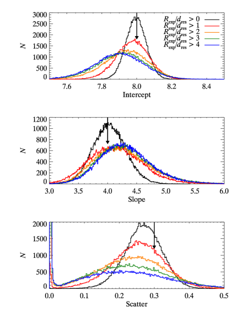
First, we use various cuts in $R_{\mathrm{infl}}/d_{\mathrm{res}}$ to eliminate galaxies from the simulated sample. The results from this simulation are shown in Figure 8. Without the Galaxy, the trends are simple and monotonic: increasing the $R_{\mathrm{infl}}/d_{\mathrm{res}}$ cutoff increases the value of the intercept and decreases the values of the slope and scatter. Because our sample RS (see Appendix B) omits the Galaxy, comparison of the orange curve to the black curve in Figure 8 approximates comparison of the fit values in our RS sample to our S sample. They show the same trends in intercept, slope, and scatter.

Figure 8.— Histograms of fit parameters from Monte Carlo simulations of $10^{5}$ realizations of 40 galaxies with BH masses derived from a model with $\alpha=8$, $\beta=4.0$, and $\epsilon_{0}=0.3$ with rms measurement errors in log mass of $0.2$. The right-hand panels differ from the left panels in that one of the 40 galaxies generated by the Monte Carlo procedure is replaced by a galaxy having the mass and velocity dispersion of the Milky Way. The black curves show results when all galaxies are included in the fits. These curves show that our fit method is able to recover the original parameters with a slight bias to lower intrinsic scatter. The remaining curves come from imposing a cutoff in $R_{\mathrm{infl}}/d_{\mathrm{res}}$ and fitting the remaining galaxies from the original 40. The colors correspond to a cutoff value of 1.0 (red), 2.0 (orange), 3.0 (green), and 4.0 (blue). The biases in the left panels can be summarized as follows: (1) the intercept $\alpha$ increases monotonically with increasing cutoff in $R_{\mathrm{infl}}/d_{\mathrm{res}}$; (2) the slope $\beta$ decreases monotonically with increasing cutoff; and (3) the intrinsic scatter $\epsilon_{0}$ decreases monotonically with increasing cutoff, with a large number of samples consistent with $\epsilon_{0}=0$. The orange curve ($R_{\mathrm{infl}}/d_{\mathrm{res}}>1$) may be compared with our fits to sample RS, which does not contain the Galaxy. If our Galaxy is included (right panels), the biases are (1) the intercept increases monotonically with increasing cutoff in $R_{\mathrm{infl}}/d_{\mathrm{res}}$, though the presence of the Galaxy mitigates this somewhat; (2) the slope is biased to slightly lower values for the first three cutoffs and to a slightly higher value for the highest cutoff; and (3) the inferred intrinsic scatter is biased to a lower value, with a significant number of runs consistent with $\epsilon_{0}=0$.

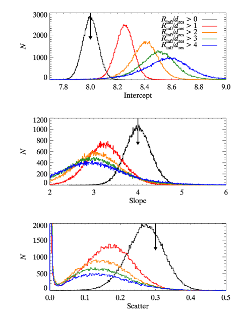
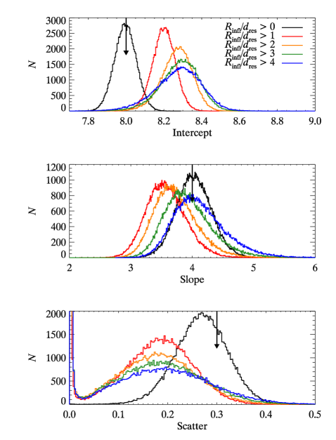
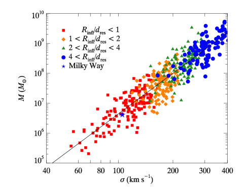
The reasons for these biases can be easily seen in Figure 9a, which illustrates the effects by plotting a sample of 500 galaxies randomly generated in the same way and plotting different ranges in $R_{\mathrm{infl}}/d_{\mathrm{res}}$ with different symbols. Because $R_{\mathrm{infl}}\approx M_{\mathrm{BH}}\sigma^{-2}$ and $M_{\mathrm{BH}}\approx\sigma^{\beta}$, lines in constant $R_{\mathrm{infl}}/d_{\mathrm{res}}$ tend to fall on lines of $M_{\mathrm{BH}}\approx\sigma^{\beta-2}$. (This argument neglects the different distances of the galaxies, but since the Monte Carlo simulation is uniformly distributed in volume, most galaxies are near the outer edge of the volume.) Since the synthesized data set uses $\beta=4.0$, each subsample has a decreased scatter because the cuts fall along lines with slope $\beta-2=2.0$ and take out the bottom portion of the scatter. The slopes are similarly biased to low values because the points have been removed from systematically smaller masses and systematically smaller velocity dispersions. The intercept increases as each subsample’s mean increases.

Figure 9.— Monte Carlo sample of 500 galaxies with BH mass generated from an $M$–$\sigma$ relation with $\alpha=8$ and $\beta=4.0$ and a log-normal scatter of 0.3 dex with measurement errors of 0.2 dex. The ridge line of the $M$–$\sigma$ relation is drawn as a black line. The Galaxy is plotted as a pentagram. Both panels use different colors and symbols for different resolution levels. The left panel defines $R_{\mathrm{infl}}=GM_{\mathrm{BH}}/\sigma^{2}$ with $M_{\mathrm{BH}}$ equal to the measured BH mass; and the right panel uses our alternate definition using the expected mass of the BH based on the $M$–$\sigma$ relation. For each definition, the symbols are $R_{\mathrm{infl}}/d_{\mathrm{res}}<1.0$ (red squares), $1.0<R_{\mathrm{infl}}/d_{\mathrm{res}}<2.0$ (orange diamonds), $2.0<R_{\mathrm{infl}}/d_{\mathrm{res}}<4.0$ (green triangles), and $R_{\mathrm{infl}}/d_{\mathrm{res}}>4.0$ (blue circles). In the left panel, fitting the combined subsamples with $R_{\mathrm{infl}}/d_{\mathrm{res}}$ exceeding a given value yields a shallower slope and a smaller intercept than the underlying $M$–$\sigma$ relation.. The reason for the bias in slope is that cuts in $R_{\mathrm{infl}}$ tend to fall along lines of $M_{\mathrm{BH}}\propto\sigma^{\beta-2}$ (since $R_{\mathrm{infl}}\propto M_{\mathrm{BH}}\sigma^{-2}$ and $M_{\mathrm{BH}}\propto\sigma^{\beta}$). This is illustrated by the dashed line of slope 2.0. Cuts using the expected $R_{\mathrm{infl}}$ (right panel) do not suffer from this bias because the cuts in $R_{\mathrm{infl}}/d_{\mathrm{res}}$ with this definition tend to run at constant $\sigma$. The bias they introduce is far less than with the traditional definition. The uncertainties in the parameters when fitting, however, are much larger due to the decreased dynamic range in $\sigma$.

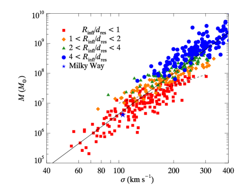
When the Galaxy is included (Fig. 8b), the magnitude of the biases decreases. The intercepts are still biased to high values. The slopes are biased to low values except those from the most restrictive cutoff, which are biased to a slightly higher value. The scatters are biased to a smaller value; a significant number are consistent with $\epsilon_{0}=0$. The bias when using older, lower values for our Galaxy’s BH mass (Ghez et al., 2005) would have produced more extreme changes in slopes.

4.4. Culling the Simulated Sample Based on Sphere of Influence from Expected Black Hole Mass

For the second culling strategy, we adopt a different definition of $R_{\mathrm{infl}}$ that does not lead to the extreme biases seen above. Because the traditional definition of $R_{\mathrm{infl}}$ depends on the measured BH mass, it is sensitive to whether the BH is overmassive or undermassive for a given velocity dispersion. Thus, using $R_{\mathrm{infl}}$ as a sample criterion necessarily biases any measurement in scatter. Instead, we offer an alternative definition based on the expected value of $M_{\mathrm{BH}}$ from the $M$–$\sigma$ relation. That is, we replace culling based on $R_{\mathrm{infl}}/d_{\mathrm{res}}$ by culling based on $R_{\mathrm{exp}}/d_{\mathrm{res}}$, where $R_{\mathrm{exp}}=GM_{\mathrm{pred}}\sigma^{-2}$ and $M_{\mathrm{pred}}=10^{\alpha}(\sigma/200~{}~{}\mathrm{km~{}s^{-1}})^{\beta}~{}{\rm M}_{\scriptscriptstyle\odot}$. Using this as a selection criterion for finding the $M$–$\sigma$ relation requires only a simple and rapidly convergent iterative procedure. It is possible that this procedure will not always converge to a unique answer, but this is unlikely to happen if the initial guess is chosen close to the actual relation. Adopting this strategy substantially decreases the bias in the fitting parameters (Fig. 10) but dramatically increases their uncertainties since the range of $\sigma$ used in the fit is reduced. The reason for this is seen in the right panel of Figure 9. Instead of falling along lines of slope 2.0, the cuts tend to fall on lines of constant $\sigma$.

Figure 10.— Histograms of fit parameters from Monte Carlo simulations as in Figure 8, except the cuts are based on $R_{\mathrm{exp}}/d_{\mathrm{res}}$ as defined in § 4.4. The colors correspond to a cutoff value of 1.0 (red), 2.0 (orange), 3.0 (green), and 4.0 (blue). The biases in the left panels are minimal, but the efficiency of recovering the original parameters is greatly reduced since the dynamic range in $\sigma$ is greatly reduced. In the right panels, the biases incurred from these cutoffs are small, and the efficiency of recovering the original parameters is greatly improved compared to the left panels since the dynamic range in $\sigma$ always includes the Galaxy. There is, however, still a tendency to infer an intrinsic scatter consistent with $\epsilon_{0}=0$ when making a large cut.

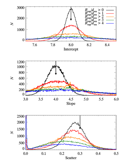
4.5. Culling Based on Traditional Sphere of Influence Using Observed Sample with Simulated Masses

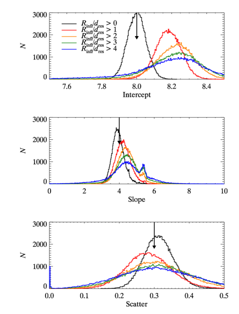
The above synthetic datasets represent an idealized scenario in which the galaxies come from a volume-limited sample. The real sample of BH mass measurements, however, is not uniformly distributed in volume. As a final experiment on a synthetic data set, we use the observed sample of velocity dispersions, errors in velocity dispersion, distances, errors in mass measurements, and instrumental resolution. The masses are synthesized from an $M$–$\sigma$ model as before and censored according to $R_{\mathrm{infl}}/d_{\mathrm{res}}$ as calculated from the synthesized BH mass. There is no need to artificially include the Galaxy in these simulations since it is used along with all of the other data. The resulting distributions of fit parameters are presented in Figure 11. Again, using the entire sample recovers the input parameters. Cuts in $R_{\mathrm{infl}}/d_{\mathrm{res}}$ show the same bias to high values of intercept as well as reducing the efficiency of the estimates. The slope is biased to high values. The intrinsic scatter is similarly biased to low values, with a noticeable number of realizations recovering zero intrinsic scatter. We plot 5 realizations and indicate their level of resolution in Figure 12. The same trends as seen in the idealized simulations are present. The trends in parameter estimation from culled samples seen here may explain why Ferrarese & Ford (2005) find a higher intercept ($\alpha=8.22\pm 0.06$), a much higher slope ($\beta=4.86\pm 0.43$), and a “negligible” scatter with their sample restricted to $R_{\mathrm{infl}}/d_{\mathrm{res}}>1$.

Figure 11.— Histograms of fit parameters from Monte Carlo simulations as in Figure 8, except that the velocity dispersions, distances, and errors in mass measurements are all derived from the actual observed sample of galaxies. The masses are synthesized from an $M$–$\sigma$ model.

Figure 12.— Same as Figure 9, except that the velocity dispersions, distances, and errors in mass measurements are all derived from the actual observed sample of galaxies. The masses are synthesized from an $M$–$\sigma$ model.

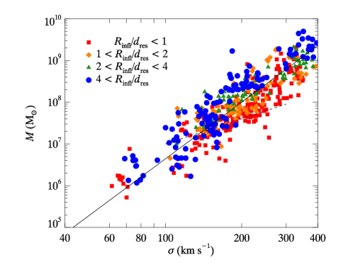
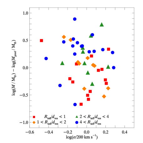
The systematic effects of $R_{\mathrm{infl}}/d_{\mathrm{res}}$ cutoffs can also be seen in Figure 13, which plots the residuals to our $M$–$\sigma$ fit as a function of $\sigma_{e}$. The lower resolution objects tend to be found toward the bottom and right of the plot, and the most highly resolved galaxies clearly show a residual trend in $\sigma_{e}$ even though the sample as a whole shows no such trend. Hence, eliminating reliable BH mass measurements (in the sense that the error bars accurately reflect the uncertainty in the measurement, even if they are large) by selecting on $R_{\mathrm{infl}}/d_{\mathrm{res}}$ will bias the resulting fits. This bias could be mitigated by using $R_{\mathrm{exp}}$ rather than $R_{\mathrm{infl}}$ in the culling criterion but then the uncertainties in the fit become much larger. Thus, our recommendation is to include BH masses without regard to the value of $R_{\mathrm{infl}}/d_{\mathrm{res}}$.

Figure 13.— Residuals in mass from our fit to $M$–$\sigma$ for the full sample. The colors and shapes of the subsamples correspond to how well resolved the BH’s sphere of influence is (from low to high $R_{\mathrm{infl}}/d_{\mathrm{res}}$: red squares, orange diamonds, green triangles, and blue circles). Removing the more poorly resolved objects from the sample leaves a residual trend, even though there is no such trend for the sample as a whole.

5. Discussion

5.1. Systematic Uncertainties in Measurements of BH Mass

Our measurements of the intrinsic scatter in the $M$–$\sigma$ and $M$–$L$ relations assume that the stated errors in $M_{\mathrm{BH}}$ accurately reflect the measurement uncertainties. If unaccounted systematic errors are large, however, they will significantly increase the inferred intrinsic scatter. We list some potential sources of systematic errors in $M_{\mathrm{BH}}$ measurements.

• Models in which the value of $\chi^{2}$ i smuch larger than the number of parameters are inadequate. We have removed $M_{\mathrm{BH}}$ measurements from our sample where this is a problem.

• For more massive galaxies, the derived stellar mass-to-light ratio ($\Upsilon_{*}$) may be wrong due to an un-modeled contribution of the dark matter halo to the stellar kinematics at the large radii used to constrain the stellar population. If the dark matter halo is less centrally concentrated than the stellar mass distribution, as is expected from cosmological simulations of adiabatic collapse (Gnedin et al., 2004), then the intrinsic $\Upsilon_{*}$ would be lower than inferred, implying larger than estimated $M_{\mathrm{BH}}$ values (Gebhardt & Thomas, 2009).

• If the BH mass is measured by gas kinematics, uncertainty in inclination and non-gravitational forces may cause systematic errors (Ho et al., 2002).

• Galaxies that have recently merged such as Cen A may not be in the equilibrium state that is assumed by stellar kinematic models.

• There are galaxies with AGN, whose central kinematics are hard to measure. This is systematic noise since it depends on how one handles the AGN subtraction.

• Uncertain deprojection of the gas density profiles may be a source of systematics.

5.2. The Value of the Slope in the $M$–$\sigma$ Relation

The slope we report here ($\beta=4.24\pm 0.41$) is noticeably, though not significantly, steeper than the slope obtained by Tremaine et al. (2002) ($\beta=4.00\pm 0.31$). For comparable assumptions, however, this difference disappears. The most direct comparison is to apply the symmetric least-squares fitting method of Tremaine et al. (2002, see Table 3) to our sample without upper limits, which yields $\beta=4.02\pm 0.37$, compared to $\beta=4.00\pm 0.31$ found by Tremaine et al. (2002). The two slopes are consistent with each other.

5.3. The Value of the Scatter in the $M$–$\sigma$ Relation

The value of the intrinsic scatter obtained here ($\epsilon_{0}=0.44\pm 0.06$) is significantly larger than the value estimated by Tremaine et al. (2002), which was no more than $\epsilon_{0}=0.25$ to $0.3$. Since the primary interest of the $M$–$\sigma$ relation derives from its tightness, a conclusion that the scatter is larger than previously believed warrants attention. Tremaine et al. (2002) used both a different fitting method and a different sample. We examine both of these, finding that the sample differences, rather than the fitting method or updated $M_{\mathrm{BH}}$ measurements for a given galaxy, are the cause of the different scatter measurements.

We fitted several different samples: (1) the original Tremaine et al. (2002) sample, (2) the Tremaine et al. (2002) sample updated to the values used in this paper, (3) sample S from this paper, and (4) galaxies in sample S that are not in Tremaine et al. (2002). Fits were done using both the maximum likelihood method developed for this paper and the symmetric least-squares method used by Tremaine et al. (2002). We use our sample without upper limits to make the most direct comparison between the methods. The intrinsic scatter that we find in sample S is almost identical to that in sample SU. When used on the same sample, there was never a significant difference between the two methods, which leads us to quote only the results from the maximum likelihood method of this paper. The original Tremaine et al. (2002) sample yields an intrinsic scatter of $\epsilon=0.31\pm 0.06$. Updating the values in the same sample increases the intrinsic scatter to $\epsilon=0.35\pm 0.06$. The intrinsic scatter in sample S is $\epsilon=0.43\pm 0.06$, and the intrinsic scatter from just the 19 galaxies in sample S not found in Tremaine et al. (2002) is $\epsilon=0.51\pm 0.11$. Since the two methods used do give consistent results, they cannot be the source of the difference.

Next we examine the difference between the original Tremaine et al. (2002) sample and the new galaxies. Kolmogorov-Smirnov tests on the distributions of mass, velocity dispersion, and error in logarithmic mass cannot rule out the null hypothesis that the two samples came from the same parent distribution at better than 50% confidence.

A chi-square test on the distribution of morphological types, however, reveals that the probability that the two samples in galaxy type come from the same parent distribution is only approximately 20%. This is far from conclusive, but it is noteworthy that the more recent $M_{\mathrm{BH}}$ measurements consist of a relatively larger number of spirals. In § 3.1, we find that the intrinsic scatter in the population of late-type galaxies may be larger than the scatter in early-type galaxies. This may be a result of unrecognized systematic effects in $M_{\mathrm{BH}}$ measurement of spirals or because the scatter is actually larger. In contrast, we find consistent intrinsic scatter estimates, at about 0.3, when fitting only early-type galaxies from the two samples.

In this context, Hu (2008) has noted that pseudobulges appear to host relatively smaller black holes than do “classical” bulges. We have included both bulge types in the analysis, and the differences in the relative contributions of the two types between various samples may enhance the intrinsic scatter.

One of the spiral galaxies that was not included in the Tremaine et al. (2002) samples is Circinus, the largest outlier in our sample. When we exclude Circinus from sample S, the scatter reduces to $\epsilon=0.36\pm 0.05$, in near agreement with Tremaine et al. (2002). While it is disturbing that a single galaxy can cause such a large change in our scatter estimates, Circinus is an extreme outlier, a factor of $\sim 30$ below the $M$–$\sigma$ ridge line. In order for any $M$–$\sigma$ model to explain such an outlier that does not have large measurement errors, a large intrinsic scatter is needed.

We summarize the reasons for the difference in intrinsic scatter measurements as follows.

• The difference in fitting methodology is not the source of the difference in intrinsic scatter estimates.

• The difference in samples is the source of the difference.

• Updating the $M_{\mathrm{BH}}$ measurements of galaxies in Tremaine et al. (2002) slightly increases the intrinsic scatter estimate.

• The galaxies in the Tremaine et al. (2002) sample and the new galaxies in this sample possibly have different distributions of Hubble types. If they do, the increased fraction of spirals in the newly added galaxies may be a source of the increased scatter. The underlying cause may be either because (1) spiral galaxies are susceptible to more systematic error or (2) there is a larger intrinsic scatter in $M_{\mathrm{BH}}$ in spiral galaxies, as might occur if there is a significant difference in the population of black holes hosted by pseudobulge versus classical bulges.

• When considering only early-type galaxies, the scatter values of the samples are consistent with each other and are close to the value quoted by Tremaine et al. (2002).

• The inclusion of Circinus makes a large difference in the scatter estimates.

5.4. The Role of Upper Limits

Upper limits provide information on the population of BH masses. Weak upper limits provide little information, but when the limit is comparable to detected BH masses at a similar velocity dispersion or luminosity, it can provide a valuable constraint on the fit. Thus, excluding upper limits from the fit excludes potentially useful information. Since restrictive upper limits will lie at lower masses, excluding them may also introduce a bias, especially in estimates of the intrinsic scatter and intercept. For these reasons, we view our fit including upper limits as the most complete answer. To avoid being biased by upper limits measured in galaxies with no BH, which do not belong in either the $M$–$\sigma$ or $M$–$L$ relations, we include the probability of a galaxy’s having no BH ($P_{\emptyset}$) in our fit. As the simplest possible form, we assume $P_{\emptyset}$ is constant for all galaxies. Given that smaller galaxies may be less likely to form central BHs and that their smaller escape velocities mean ejection of their BHs is more likely, this assumption may not hold. Tests using a simple linear dependence on velocity dispersion, $P_{\emptyset}=\zeta+\eta\log{(\sigma/200~{}\mathrm{km~{}s^{-1}})}$, found $\eta=0.001\pm 0.047$. So assuming a constant form is unlikely to introduce a strong bias, and in any event the data are not strong enough to support a more elaborate model. Excluding upper limits reduces the slope, although not by a statistically significant amount.

5.5. Implications for Space Density of Black Holes and Studies of $M$–$\sigma$ Evolution

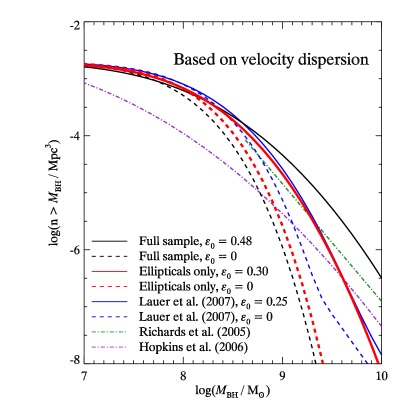
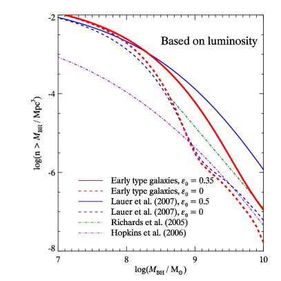
The intrinsic scatter in BH mass scaling relations affects estimates of the space density of BHs based on velocity dispersion or luminosity functions (Yu & Tremaine, 2002; Marconi et al., 2004; Lauer et al., 2007b). This is especially true for the largest BHs. The fundamental reason is that most of the largest BHs will come from lower dispersion or lower luminosity hosts with overmassive BHs. We reproduce the cumulative density functions based on our results in Figure 14. In order to calculate the density of BHs, a predictor for $M_{\mathrm{BH}}$ is needed, which requires a regression on $\sigma_{e}$ or $L_{V}$. Our maximum-likelihood method may be used to do a regression by simply setting the uncertainties in $\sigma_{e}$ and $L_{V}$ to zero. The resulting fits differ very little from those presented above.

Figure 14 shows that there is a marked difference in the space density of BHs when assuming no scatter or our best-fit scatter. Regressions for both the entire sample and for ellipticals-only are shown in the left panel of Figure 14. Because the largest BHs are found in elliptical galaxies, the ellipticals-only curve with scatter best reflects the velocity-dispersion-based calculation in this paper. Lauer et al. (2007b) argued that the more fundamental scaling relation for the largest BHs may be $M$–$L$. If this is the case, then the curve for early-type galaxies with scatter in the right-hand panel of Figure 14 is the appropriate function to use. The difference between the two curves at the high-mass end is considerable, and it is a reflection of the inconsistency of the $M$–$\sigma$ and $M$–$L$ relations in this regime. Studies of the evolution of $M$–$\sigma$ are also biased due to the high scatter.

Figure 14.— BH space density derived from velocity dispersion (left) and luminosity (right) of the host galaxy. The curves show logarithmic cumulative density for different assumptions. The curves are the BH mass functions based on (left) the SDSS velocity dispersion function (Sheth et al., 2003) and (right) a fit of SDSS data to the Schechter (1976) luminosity function fit (Blanton et al., 2003) augmented by the brightest cluster galaxies of Postman & Lauer (1995). Predictions of BH mass based on velocity dispersion (left) and luminosity function (right) are from fits to all galaxies in this paper (orange) and to elliptical galaxies in this paper (red). We also plot corresponding predictions from Lauer et al. (2007b) (blue). Dashed lines indicate mass functions assuming no intrinsic scatter, and solid lines show mass functions assuming the best-fit value of the intrinsic scatter. For reference, both panels show alternate density calculations. The magenta dot-dashed line is based on the Richards et al. (2005) luminosity function from SDSS at a redshift of $z=2.5$, assuming (1) a bolometric correction of 6.5 (Elvis et al., 1994; Sazonov et al., 2004), (2) that the AGN are accreting at their Eddington limit, and (3) that the AGN have a duty cycle of 0.03 (Steidel et al., 2002). The purple dot-dashed line is the quasar model due to Hopkins et al. (2006a). The differences between the solid and dashed curves of the same color show the large discrepancy between considering and omitting intrinsic scatter in estimating the density of the BHs. The red, solid curves in both panels show the best-fit results from this paper.

6. Conclusions

In this work we have presented the latest results relating the mass of a galaxy’s central BH with the stellar velocity dispersion and bulge luminosity of the galaxy.

(1) Most current $M$–$\sigma$ fit. We compiled 49 BH mass measurements and fit a new $M$–$\sigma$ relation using a maximum-likelihood method that includes an intrinsic scatter component. We also include 18 upper limits to BH masses. The best fit for the relation is

$$\log{\left(\frac{M_{\mathrm{BH}}}{{\rm M}_{\scriptscriptstyle\odot}}\right)}=(8.12\pm 0.08)+(4.24\pm 0.41)\log{\left(\frac{\sigma_{e}}{200~{}~{}\mathrm{km~{}s^{-1}}}\right)},$$ (7)

with an intrinsic rms Gaussian scatter of $\epsilon_{0}=0.44\pm 0.06$.

(2) Characterization of the intrinsic scatter in $M$–$\sigma$. Study of the distribution of BH masses in galaxies in a narrow range in velocity dispersion reveals that the intrinsic scatter in the $M$–$\sigma$ relation is consistent with log-normal in BH mass and inconsistent with normal in BH mass. Further, we find no evidence that adopting a log-quadratic, rather than a log-linear, relation between BH mass and velocity dispersion reduces the scatter.

(3) Smaller scatter in the population of ellipticals. When we limit our sample to include elliptical galaxies, we find that the scatter decreases to $\epsilon_{0}=0.31\pm 0.06$. This is $\sim 2\sigma_{68}$ smaller than the intrinsic scatter in non-elliptical galaxies, $\epsilon_{0}=0.53\pm 0.10$. If real, this difference could either be because of larger systematic errors in BH mass determinations of late-type galaxies or because elliptical galaxies lie closer to the $M$–$\sigma$ relation ridge line.

(4) Most current $M$–$L$ fit. We also fit a relation between the mass of the central BH and the $V$-band bulge luminosity of the host. The best-fit for the relation is

$$\log{\left(\frac{M}{{\rm M}_{\scriptscriptstyle\odot}}\right)}=(8.95\pm 0.11)+(1.11\pm 0.18)\log{\left(\frac{L_{V}}{10^{11}{\rm L}_{{\scriptscriptstyle\odot},V}}\right)}$$ (8)

with an intrinsic scatter of $\epsilon_{0}=0.38\pm 0.09$.

(5) Characterization of the scatter in $M$–$L$ fit. We also find through study of the distribution of BH masses in galaxies in a narrow range of bulge luminosity that the scatter is adequately described by a log-normal intrinsic scatter in BH mass and is inconsistent with a distribution normal in mass.

(6) Identification of bias in samples that use $R_{\mathrm{infl}}/d_{\mathrm{res}}$ as a selection criterion. Selecting a sample for fitting an $M$–$\sigma$ relation with a minimum value of $R_{\mathrm{infl}}/d_{\mathrm{res}}$ causes a bias that leads to an overestimate of the intercept, an overestimate estimate of the slope, and an incorrect estimate of the intrinsic scatter. The bias arises because $R_{\mathrm{infl}}\approx GM_{\mathrm{BH}}\sigma^{-2}$ and $M_{\mathrm{BH}}\approx\sigma^{4}$ so that $R_{\mathrm{infl}}\approx\sigma^{2}$. Thus, cuts in constant $R_{\mathrm{infl}}/d_{\mathrm{res}}$ systematically remove BH masses from the low-mass and low-velocity-dispersion portion of the $M$–$\sigma$ plane. For this reason, we exclude only those BH mass measurements that we believe to be unreliable.

(7) Implications for space density of BHs. Our findings that the intrinsic scatter in the $M$–$\sigma$ for ellipticals and $M$–$L$ relations for early-type galaxies are $\epsilon_{0}=0.31\pm 0.06$ and $\epsilon_{0}=0.38\pm 0.09$, respectively, have an important influence on the determination of the space density of the most massive BHs. We find that the density of BHs with $M_{\mathrm{BH}}>3\times 10^{9}~{}{\rm M}_{\scriptscriptstyle\odot}$ is $8\times 10^{-7}~{}\mathrm{Mpc^{-3}}$ (based on the $M$–$\sigma$ relation) and $\sim 3\times 10^{-6}~{}\mathrm{Mpc^{-3}}$ (based on the $M$–$L$ relation).

Appendix A Fitting Method

In this Appendix we describe our fitting method. Previous methods used for this problem include the Akritas & Bershady (1996) extension of the least-squares estimator (Ferrarese & Merritt, 2000) and a symmetric $\chi^{2}$ method (Tremaine et al., 2002). Neither of these methods, however, can incorporate upper limits naturally. We use two general methods for fitting the $M$–$\sigma$ relation in this paper: (1) the symmetric $\chi^{2}$ method of Tremaine et al. (2002), and (2) a generalized maximum-likelihood method developed for this work. We include the symmetric $\chi^{2}$ method for comparison to Tremaine et al. (2002), but the maximum likelihood method more naturally includes an intrinsic scatter component and more naturally incorporates upper limits.

We consider several functional forms for the measurement error distribution and for the intrinsic scatter, both because it is far from clear that the conventional log-normal distribution accurately describes either distribution, and because distributions with fatter tails than normal tend to handle outliers more robustly. In §§ A.2-A.6 we describe our various assumptions about the error distribution and scatter.

Ultimately, based on tests described in Appendix B below, we find that the choice of error distribution does not significantly change the fitted slope, intercept, or scatter; thus, we adopt the results from the fit with Gaussian distributions as the most straightforward.

We take the measurement error in logarithmic mass to be $0.5[\log{(M_{\mathrm{high}})}-\log{(M_{\mathrm{low}})}]$, where $M_{\mathrm{high}}$ and $M_{\mathrm{low}}$ are the published bounds to the 1$\sigma$ range in BH mass. Even though some of the galaxies in our sample have asymmetric errors (i.e., $M_{\mathrm{BH}}-M_{\mathrm{low}}\not=M_{\mathrm{high}}-M_{\mathrm{BH}}$), we interpret the errors to be symmetric in logarithmic mass. This is a shortcoming of our methods, which should be remedied in future work. For the sake of consistency, we interpret the errors to be the 68% confidence intervals regardless of the form of the error distribution, as described below. In our sample, IC 1459 and NGC 1399 each have two mass measurements that are marginally inconsistent yet reliable. To account for this we include both measurements and weight each half as much.

Similar to the measurement errors in BH mass, we take the magnitude of the intrinsic scatter to be the interval that contains 68% of the area under the curve, regardless of the shape of the intrinsic scatter. We further assume (1) that the shape of the intrinsic scatter is symmetric above and below the ridge line, and (2) that the magnitude of the intrinsic scatter is independent of velocity dispersion.

A.1. Maximum-Likelihood Method for Parameter Estimation

Let $P\left(\mu|s\right)$ be the probability that there is a BH of logarithmic mass $\mu\equiv\log{\left(M/{\rm M}_{\scriptscriptstyle\odot}\right)}$ given galaxy properties $s$. For our fits, $s$ is either the logarithm of the velocity dispersion $s=\log{(\sigma/200~{}~{}\mathrm{km~{}s^{-1}})}$ or the logarithm of the luminosity $s=\log{(L_{V}/10^{11}{\rm L}_{{\scriptscriptstyle\odot},V})}$. Thus, $P\left(\mu|s\right)$ is either the $M$–$\sigma$ or $M$–$L$ relation. Given a set of observations chosen on the basis of $s$ (or other properties not correlated with BH mass), the likelihood of a set of observed points $\left\{\mu_{i},s_{i}\right\}$ is the product of the likelihood of each pair of measurements $\ell_{i}=\ell\left(\mu_{i},s_{i}\right)$:

$${\mathcal{L}}=\prod_{i}\ell_{i}.$$ (A1)

In the absence of measurement errors

$$\ell_{i}=P\left(\mu_{i}|s_{i}\right).$$ (A2)

For a given observation, the probability of measuring a mass between $\mu_{\rm obs}$ and $\mu_{\rm obs}+d\mu_{\rm obs}$ in galaxy $i$, given that the actual BH mass in this galaxy is $\mu$, is $Q_{i}(\mu_{\rm obs}|\mu)d\mu_{\rm obs}$, normalized so that the integral over all $\mu_{\rm obs}$ is unity. Then equation (A2) becomes

$$\ell_{i}=\ell(\mu_{i},s_{i})=\int_{{\mathrm{all}\ }\mu}Q_{i}\left(\mu_{i}|\mu\right)P\left(\mu|s_{i}\right)d\mu.$$ (A3)

Note that equation (A3) reduces to equation (A2) if $Q_{i}(\mu_{i}|\mu)=\delta(\mu-\mu_{i})$. We also include observational upper limits to BH masses in our fits. In doing so, we must also allow for the possibility that some galaxies have no BH; otherwise, a single galaxy with no BH and a strong observational upper limit could strongly bias our parameter fits. To take this into account, we modify equation (A3) to be

$$\ell_{i}=P_{\emptyset}Q_{i}(\mu_{i}|-\infty)+(1-P_{\emptyset})\int_{\mathrm{all}\ \mu}Q_{i}\left(\mu_{i}|\mu\right)P(\mu|s_{i})d\mu,$$ (A4)

where $P_{\emptyset}$ is the probability of the galaxy having no BH. In all cases $P_{\emptyset}$ is consistent with zero, with typical estimates of $P_{\emptyset}=0.003\pm 0.03$.

In the following sections we consider specific forms for $Q_{i}(\mu_{i}|\mu)$ and $P(\mu|s_{i})$.

A.2. Gaussian Error Distribution with Gaussian Scatter

Let $G_{\epsilon}(x_{1}-x_{2})\equiv(1/\epsilon\sqrt{2\pi})\exp{[-(x_{1}-x_{2})^{2}/2\epsilon^{2}]}$ be a normalized Gaussian with dispersion $\epsilon$. Then suppose

$$P\left(\mu|s_{i}\right)=G_{\epsilon_{0}}\left(\mu-f(s_{i})\right),$$ (A5)

where $f$ is a ridge line through the joint distribution in $\mu$ and $s$. That is, $f$ is the $M$–$\sigma$ or the $M$–$L$ relation that we are considering. We refer to $\epsilon_{0}$ as the cosmic or intrinsic scatter in the relation, and we assume it to be independent of all galaxy properties. Then

$$\ell_{i}=\int Q_{i}\left(\mu_{i}|\mu\right)G_{\epsilon_{0}}\left(\mu-f(s_{i})\right)d\mu.$$ (A6)

If $Q_{i}$ is normally distributed about $\mu_{i}$ (i.e., the error in measured logarithmic BH mass is Gaussian) so that

$$Q_{i}=G_{\epsilon_{i}}\left(\mu_{i}-\mu\right),$$ (A7)

where $\epsilon_{i}$ is the measurement error, then

$$\ell_{i}=\int G_{\epsilon_{i}}\left(\mu_{i}-\mu\right)G_{\epsilon_{0}}\left(\mu-f(s_{i})\right)d\mu.$$ (A8)

Equation (A8) is a convolution of two Gaussians — itself a Gaussian with variance equal to the sum of the two variances:

$$\ell_{i}=G_{\sqrt{{\epsilon_{i}}^{2}+{\epsilon_{0}}^{2}}}\left(\mu_{i}-f(s_{i})\right).$$ (A9)

Equation (A9) is the justification for adding cosmic scatter to the measurement error in Tremaine et al. (2002). We refer to this model as Gaussian error distribution with Gaussian intrinsic scatter (GG; see Table 2 for a list of abbreviations for models and samples). This is the method we use for our final values of the parameters in the $M$–$\sigma$ and $M$–$L$ relations.

Table 2List of Abbreviations Used

Abbrev.	$Q_{i}(\mu)$	$P_{i}(\mu)$	Short Description
GG	A9	A5	Gaussian error distribution with Gaussian intrinsic scatter
CG	A12	A5	Constant probability errors with Gaussian intrinsic scatter
DG	A14	A5	Double-sided exponential errors with Gaussian intrinsic scatter
DD	A14	A15	Double-sided exponential errors
			with double-sided exponential intrinsic scatter
LG	A16	A5	Lorentzian errors with Gaussian intrinsic scatter
LL	A16	A17	Lorentzian errors with Lorentzian intrinsic scatter
SU			Full sample with upper limits
S			Sample without upper limits
RS			Restricted sample, no upper limits

Note. — List of abbreviations. Column 1 gives the abbreviation. For the maximum-likelihood method abbreviations, Columns 2 and 3 give the equation numbers that describe the measurement error distribution $Q_{i}(\mu)$, and the intrinsic scatter distribution $P_{i}(\mu)$, respectively, while Column 4 gives a short description.

A.3. Upper Limits

To include upper limits, we note that the probability that a galaxy with properties $s$ has a logarithmic BH mass greater than $\mu_{u}$ is

$$U(\mu_{u}|s)=(1-P_{\emptyset})\int_{\mu_{u}}^{\infty}P(\mu|s)d\mu.$$ (A10)

Suppose that an observation indicates the mass of the BH in a given galaxy is less than $\mu_{u}$ at the $n\sigma_{68}$ level. This means that the mass is greater than $\mu_{u}$ with probability $\delta_{n}$ and less than $\mu_{u}$ with probability $1-\delta_{n}$, where $\delta_{1}=0.159$, $\delta_{2}=0.0228$, $\delta_{3}=0.00135$, etc. To include the upper limits in the maximum-likelihood method, we must include the possibility that the observation has incorrectly concluded that the mass is less than $\mu_{u}$, which will happen a fraction $\delta_{n}$ of the time. Then the likelihood of observing an upper limit of mass $\mu_{u}$ at the $n\sigma_{68}$ level in a galaxy with property $s$ is

$$\ell_{i}=\delta_{n}U(\mu_{u}|s)+(1-\delta_{n})[1-U(\mu_{u}|s)].$$ (A11)

A.4. Constant Probability

We may also decide that a mass measurement means the mass is restricted between $\mu_{1}$ and $\mu_{2}$, but that there is no preferred mass in that range. We may assume this, for example, because we believe that the published error bars are a reasonable estimate of the uncertainty in BH mass, but the error distribution is unknown. In this case, $Q_{i}$ is a constant $C$, and

$$\ell_{i}=C\int_{\mu_{1}}^{\mu_{2}}G_{\epsilon_{0}}\left(\mu-f(s_{i})\right)d\mu$$ (A12)

with

$$C=\frac{1}{\mu_{2}-\mu_{1}},$$ (A13)

where the normalization arises since the integral of $Q_{i}$ over all $\mu_{i}$ should be unity. In order to maintain the consistency of having $\epsilon_{i}$ indicate the 68% confidence limit, we take $\mu_{1,~{}2}=\mu_{i}\mp\epsilon_{i}/0.68$. We refer to this method as CG.

A.5. Double-Sided Exponential

We also use robust methods to estimate the parameters of $f(s_{i})$ by dropping the assumption of a Gaussian distribution of measurement errors in $\mu$ and, optionally, the assumption of Gaussian intrinsic scatter in $\mu$. Robust methods are, in general, more tolerant of outliers in distributions. This may be especially appropriate for our sample since the measurements come from several different groups using several different measurement methods, and the systematic errors may be larger than the intrinsic scatter. There is no a priori reason to assume that the intrinsic scatter is correctly described by a Gaussian distribution. We use two robust methods. First, we use a double-sided exponential, a standard robust method (e.g., Press et al., 1986):

$$Q_{i}(\mu_{i}|\mu)=\left(2a_{i}\right)^{-1}\exp{\left(-\left|\mu-\mu_{i}\right|/a_{i}\right)},$$ (A14)

where we determine $a_{i}$ by assuming that the quoted 1$\sigma_{68}$ measurement errors contain the 68% confidence interval and thus correspond to $-\ln{\left(0.32\right)}a_{i}$. We use this form of measurement error with either equation (A5) (DG) or with a cosmic scatter that is also described by a double-sided exponential (DD):

$$P_{i}(\mu)=\left(2a_{0}\right)^{-1}\exp{\left(-\left|\mu_{i}-f(s_{i})\right|/a_{0}\right)},$$ (A15)

where $a_{0}=-\epsilon_{0}/\ln{0.32}$.

A.6. Lorentzian

For our second robust method we use a Lorentzian to describe the error distribution of the BH mass measurements. Lorentzian distributions have large tails and thus tend to be especially tolerant of outliers:

$$Q_{i}(\mu_{i}|\mu)=\left(\frac{\Gamma_{i}}{\pi}\right)\frac{1}{\left(\mu-\mu_{i}\right)^{2}+\Gamma^{2}_{i}},$$ (A16)

where we determine $\Gamma_{i}$ by assuming the 68% confidence intervals correspond to $\tan{(0.68\pi/2)}\Gamma_{i}$. We use this form with either equation (A5) (LG) or with a cosmic scatter that is also described by a Lorentzian (LL):

$$P_{i}(\mu)=\left(\frac{\Gamma_{0}}{\pi}\right)\frac{1}{\left(\mu-f(s)\right)^{2}+\Gamma^{2}_{0}},$$ (A17)

where $\Gamma_{0}=\epsilon_{0}/\tan{(0.68\pi/2)}$.

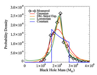
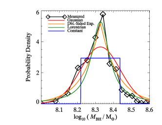
The error distributions described above are compared to the measured probability found for NGC 4026 by Gültekin et al. (2009) in Figure 15.

Figure 15.— Comparison of assumed error distributions with measured probability distribution of NGC 4026 as a function of $M_{\mathrm{BH}}$ (left) and $\log{(M_{\mathrm{BH}}/{\rm M}_{\scriptscriptstyle\odot})}$ (right). The measured probability distribution comes from the $chi^{2}$ values from Gültekin et al. (2009). The distributions are normalized so that the integral over $\log{(M_{\mathrm{BH}}/{\rm M}_{\scriptscriptstyle\odot})}$ is unity. This figure illustrates the differences among the assumed error distributions.

In practice, for all methods we minimize $-\ln{{\mathcal{L}}}$ by the downhill simplex method (e.g., Press et al., 1986). To calculate uncertainties in parameters, we change each parameter and refit (allowing the other parameters to vary to maximize $\ln{{\mathcal{L}}}$) until $\ln{{\mathcal{L}}}$ decreases by $0.5$. We also run a Monte Carlo bootstrap described in Appendix B.

A.7. Errors in the Independent Variable

Errors in the independent variables (velocity dispersion and bulge luminosity) are incorporated by Monte Carlo sampling of the independent variables. For example, for determining the $M$–$\sigma$ fit, we select values of $\sigma$ according to the measured values and uncertainties. For each fit $10^{3}$ realizations are done, and the small parameter uncertainties from this are added in quadrature.

A.8. Maximum-Likelihood Method: Model Comparison

To compare two models we calculate the odds ratio

$${\mathcal{R}_{ab}}=\frac{\int{\mathcal{L}_{a}}(a_{1},a_{2},...,a_{m})P_{a}(a_{1},a_{2},...,a_{m})da_{1}da_{2}...da_{m}}{\int{\mathcal{L}_{b}}(b_{1},b_{2},...,b_{n})P_{b}(b_{1},b_{2},...,b_{n})db_{1}db_{2}...db_{n}},$$ (A18)

where ${\mathcal{L}_{a}}$ is the likelihood of the data given model $a$ with $m$ parameters $a_{i}$, which have a prior probability distribution $P_{a}$, and similarly for model $b$. The models need not have the same number of parameters. We assume that the prior probability distributions are uniform within the ranges $[4,12]$ for intercepts [$\mu(\sigma_{e}=200~{}\mathrm{km~{}s^{-1}})$ or $\mu(L_{V}=10^{11}{\rm L}_{{\scriptscriptstyle\odot},V})$], $[-10,10]$ for slopes, and $[0,2]$ for cosmic scatter, though any reasonable set of ranges produces the same qualitative results. The integrals are calculated by the Vegas Monte Carlo method (Lepage, 1978).

Appendix B Results from Different Error Distributions, Scatter Forms, and Fit Samples

The results from $M$–$\sigma$ fits are summarized in Table 3 and plotted in Figure 16.

First, we analyze our dataset excluding upper limits (S) with the method of Tremaine et al. (2002), which consists of two distinct variants. (1) Measurement errors and intrinsic scatter are combined into a single number, the rms deviation of $\log(M_{\mathrm{BH}}/{\rm M}_{\scriptscriptstyle\odot})$ from the ridge line (denoted $\epsilon_{0}$, even though this is normally reserved for the intrinsic scatter), which is assumed to be the same for all galaxies and is determined by requiring that the reduced $\chi^{2}$ of the fit be unity. (2) The stated measurement errors and the intrinsic scatter $\epsilon_{0}$ are added in quadrature, as in Equation (A9). When using the first method, we find $\alpha=8.19\pm 0.06$ and $\beta=3.99\pm 0.37$ for $\epsilon_{0}=0.43$. When using the second method, we find $\alpha=8.19\pm 0.06$ and $\beta=4.06\pm 0.37$ for $\epsilon_{0}=0.40$. The slopes we obtain here are consistent with Tremaine et al. (2002), but the scatters are larger (see § 5.2).

Table 3Parameter Estimates for $M$–$\sigma$ Relation

Method	Sample	$\alpha$	$\beta$	$\epsilon_{0}$	$P_{\emptyset}$
T02eq	S	$8.19\pm 0.063$	$4.02\pm 0.369$	$0.41\phantom{\pm 0.000}$	…
T02eq	S	$8.19\pm 0.063$	$3.99\pm 0.369$	$0.43\phantom{\pm 0.000}$	…
T02ind	S	$8.19\pm 0.064$	$4.06\pm 0.370$	$0.40\phantom{\pm 0.000}$	…
GG	SU	$8.12\pm 0.080$	$4.24\pm 0.410$	$0.44\pm 0.059$	$0.0004\pm 0.018$
CG	SU	$8.13\pm 0.085$	$4.28\pm 0.437$	$0.45\pm 0.063$	$0.0006\pm 0.016$
DG	SU	$8.09\pm 0.088$	$4.37\pm 0.603$	$0.52\pm 0.064$	$0.0002\pm 0.015$
DD	SU	$8.18\pm 0.075$	$4.05\pm 0.382$	$0.40\pm 0.069$	$0.0001\pm 0.015$
LG	SU	$8.15\pm 0.079$	$4.16\pm 0.481$	$0.39\pm 0.068$	$0.0003\pm 0.021$
LL	SU	$8.23\pm 0.077$	$4.00\pm 0.496$	$0.35\pm 0.105$	$0.0002\pm 0.020$
GG	S	$8.18\pm 0.079$	$3.95\pm 0.423$	$0.43\pm 0.058$	…
CG	S	$8.18\pm 0.079$	$3.96\pm 0.426$	$0.43\pm 0.058$	…
DG	S	$8.15\pm 0.093$	$4.05\pm 0.507$	$0.51\pm 0.067$	…
DD	S	$8.23\pm 0.073$	$3.88\pm 0.760$	$0.39\pm 0.082$	…
LG	S	$8.21\pm 0.073$	$3.91\pm 0.676$	$0.37\pm 0.068$	…
LL	S	$8.27\pm 0.072$	$3.71\pm 0.402$	$0.32\pm 0.094$	…
GG	RS	$8.29\pm 0.078$	$3.74\pm 0.404$	$0.25\pm 0.059$	…
CG	RS	$8.30\pm 0.069$	$3.76\pm 0.369$	$0.25\pm 0.050$	…
DG	RS	$8.29\pm 0.073$	$3.71\pm 0.405$	$0.24\pm 0.059$	…
DD	RS	$8.33\pm 0.067$	$3.73\pm 0.342$	$0.20\pm 0.060$	…
LG	RS	$8.30\pm 0.083$	$3.72\pm 0.417$	$0.23\pm 0.070$	…
LL	RS	$8.38\pm 0.087$	$3.74\pm 0.708$	$0.15\pm 0.108$	…

Note. — Results from fits. The first three lines are the methods of Tremaine et al. (2002). The first line (T02) is the average of two symmetric $\chi^{2}$ variants in which intrinsic scatter is increased until $\chi^{2}$ per degree of freedom is unity, with each mass measurement either given equal weight (T02eq) or with individual errors (T02ind). Method and sample abbreviations are described in Table 2.

Figure 16.— Results of fits to the $M$–$\sigma$ relation showing best-fit intercepts ($\alpha$), best-fit slopes ($\beta$), and best-fit intrinsic scatters ($\epsilon_{0}$) against each other. The adopted fitting methods are plotted with the symbol from the legend, which uses abbreviations from Table 2. For clarity, we show representative error ellipses for method GG for each of the samples. The error ellipses are the 68% confidence limits in the joint distribution of the two parameters plotted. The sample used is indicated by the color of the parameter uncertainties: blue (sample without limits [S]), red (full sample including upper limits [SU]), and green (restricted sample [RS]). The parameter values for the various adopted methods do not significantly vary, as can be seen from the fact that most points from the same sample (same color) fall inside the uncertainty box implied by the error bars. The values from different samples, however, do vary. We discuss the reasons for the differences in sample RS (which has a cutoff in $R_{\mathrm{infl}}/d_{\mathrm{res}}$) in § 4 and for the differences when including upper limits in § 5.4.

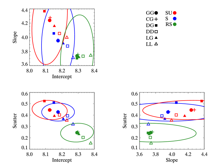
Then we use the maximum-likelihood method with the various assumed forms for measurement errors and the intrinsic scatter. Using the different error distributions for the sample that includes upper limits (SU), we find a range of intercepts from 8.09 to 8.23, which is consistent compared to the largest parameter uncertainty estimate of 0.09. Similarly, we find slopes in the range 4.00 to 4.37, a smaller range than the $\sim 0.4$ uncertainty. The estimates of the intrinsic scatter range from 0.35 to 0.52 with uncertainties of 0.06–0.11.

For the sample that does not include upper limits (S), we find a similar self-consistency among the different error and scatter distributions. The intercept is larger when excluding upper limits. The slope is shallower in the sample without limits, though not at a significant level, and the scatter is slightly (but not significantly) smaller. The consistency of the results among the different error distributions for a given sample indicates that the choice of distribution is not driving the values we obtain for parameters. The results for the restricted sample (RS) are similarly self-consistent, though compared to the full sample SU they have a larger intercept, shallower slope, and smaller intrinsic scatter, for reasons discussed in § 4. Thus, assuming a different error distribution does not have a strong effect on the results, but selecting a different sample does.

As a check on the uncertainty estimation, we calculate a bootstrap Monte Carlo of our sample. For each combination of measurement error and intrinsic scatter distributions, we randomly extract data points from the original sample with replacement for $10^{3}$ realizations and fit each sample. The bootstrap method provides a powerful way of examining whether any outlying measurements are driving the fit as well as a consistency check on uncertainty estimations. We show the distribution of best-fit parameters for two combinations of distributions: Gaussian measurement error with Gaussian intrinsic scatter (Fig. 17) and the Lorentzian measurement error with Lorentzian intrinsic scatter (Fig. 18), each with and without upper limits. Table 4 shows that in all cases the median fit parameters with 68% intervals of the distributions are very close to the values we found above. The distributions appear well approximated by a Gaussian.

Table 4Bootstrap Monte Carlo

Method	Sample	$\alpha$	$\beta$	$\epsilon_{0}$
GG	SU	$8.14\pm.07$	$4.31\pm.52$	$0.44\pm.07$
LL	SU	$8.23\pm.08$	$3.96\pm.48$	$0.33\pm.09$
GG	S	$8.17\pm.07$	$3.95\pm.36$	$0.42\pm.07$
LL	S	$8.27\pm.08$	$3.78\pm.52$	$0.31\pm.08$

Note. — Results from bootstrap fits expressed as median value. The uncertainties quoted encompass 68% of the values. Methods are as given in Table 3. The values are in very close agreement with the corresponding values given in Table 3. This indicates that the uncertainties derived from our fitting method are accurate and are not strongly influenced by outliers.

Figure 17.— Histograms of parameter estimates from the bootstrap samples assuming Gaussian measurement errors and Gaussian intrinsic scatter. Left panels are for the full sample, SU; right panels do not include upper limits (sample S). The distributions are unimodal, and the medians and 68% intervals are in good agreement with our best-fit values and uncertainties.

text

Figure 18.— Histograms of parameter estimates from the bootstrap samples assuming Lorentzian measurement errors and Lorentzian intrinsic scatter. Left panels are for the full sample, SU; right panels do not include upper limits (sample S). The distributions are unimodal, and the medians and 68% intervals are in good agreement with our best-fit values and uncertainties.

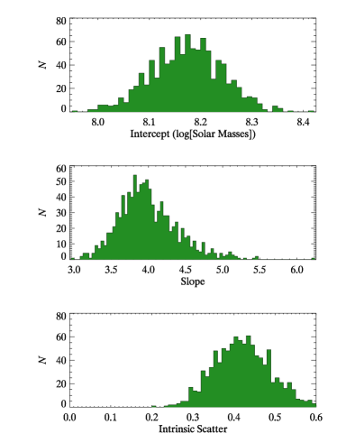
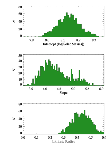
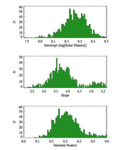
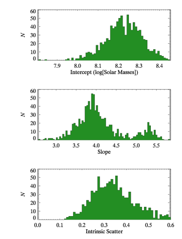
Given the consistency among the different assumptions and the consistency between the different uncertainty estimation methods, we conclude that the results are insensitive to the choice of distribution of measurement error and intrinsic scatter (so long as the “width” $\epsilon_{0}$ is consistently defined as the interval containing 68% of the distribution). The best-fit parameters of the $M$–$\sigma$ and $M$–$L$ relations, however, do depend on the sample choice. Thus, we adopt the simplest combination of measurement error and intrinsic scatter distributions, GG, for the estimates of the fit parameters and their uncertainties that we quote in the abstract.

Table 5Sample of Dynamically Detected Black Hole Masses

		Dist.	$M_{\mathrm{BH}}$	$M_{\mathrm{low}}$	$M_{\mathrm{high}}$	Method,	$\sigma_{e}$
Galaxy	Type	Mpc	${\rm M}_{\scriptscriptstyle\odot}$	${\rm M}_{\scriptscriptstyle\odot}$	${\rm M}_{\scriptscriptstyle\odot}$	Ref.	$\mathrm{km~{}s^{-1}}$		$M_{V,T}^{0}$	$M_{V,{\mathrm{bulge}}}^{0}$	${R_{\mathrm{infl}}/d_{\mathrm{res}}}$	Samp.
Circinus	Sb	4.0	$1.7\times 10^{6}$	$1.4\times 10^{6}$	$2.1\times 10^{6}$	maser,  1	$158$$\pm$	$18$	$-17.36$	. . .	6.06	S
IC1459	E4	30.9	$2.8\times 10^{9}$	$1.6\times 10^{9}$	$3.9\times 10^{9}$	stars,  2	$340$$\pm$	$17$	$-22.57$	$-22.57\pm 0.15$	0.56	S
MW	Sbc	0.008	$4.1\times 10^{6}$	$3.5\times 10^{6}$	$4.7\times 10^{6}$	stars,  3	$105$$\pm$	$20$	. . .	. . .	20622	S
N0221     M32	E2	0.86	$3.1\times 10^{6}$	$2.5\times 10^{6}$	$3.7\times 10^{6}$	stars,  4	$75$$\pm$	$3$	$-16.83$	$-16.83\pm 0.05$	12.2	RS
N0224     M31	Sb	0.80	$1.5\times 10^{8}$	$1.2\times 10^{8}$	$2.4\times 10^{8}$	stars,  5	$160$$\pm$	$8$	$-21.84$	. . .	113	S
N0821	E4	25.5	$4.2\times 10^{7}$	$3.4\times 10^{7}$	$7.0\times 10^{7}$	stars,  6	$209$$\pm$	$10$	$-21.24$	$-21.24\pm 0.13$	0.33	S
N1023	SB0	12.1	$4.6\times 10^{7}$	$4.1\times 10^{7}$	$5.1\times 10^{7}$	stars,  7	$205$$\pm$	$10$	$-21.26$	$-20.61\pm 0.28$	0.81	S
N1068     M77	Sb	15.4	$8.6\times 10^{6}$	$8.3\times 10^{6}$	$8.9\times 10^{6}$	maser,  8	$151$$\pm$	$7$	$-22.17$	. . .	22.5	S
N1300	SB(rs)bc	20.1	$7.1\times 10^{7}$	$3.6\times 10^{7}$	$1.4\times 10^{8}$	gas,  9	$218$$\pm$	$10$	$-21.34$	. . .	0.65	S
N1399	E1	21.1	$5.1\times 10^{8}$	$4.4\times 10^{8}$	$5.8\times 10^{8}$	stars, 10	$337$$\pm$	$16$	$-22.13$	$-22.13\pm 0.10$	1.82	S
N1399	E1	21.1	$1.3\times 10^{9}$	$6.4\times 10^{8}$	$1.8\times 10^{9}$	stars, 11	$337$$\pm$	$16$	$-22.13$	$-22.13\pm 0.10$	3.02	S
N2748	Sc	24.9	$4.7\times 10^{7}$	$8.6\times 10^{6}$	$8.5\times 10^{7}$	gas,  9	$115$$\pm$	$5$	$-20.97$	. . .	1.27	S
N2778	E2	24.2	$1.6\times 10^{7}$	$5.8\times 10^{6}$	$2.5\times 10^{7}$	stars,  6	$175$$\pm$	$8$	$-19.62$	$-19.62\pm 0.13$	0.45	S
N2787	SB0	7.9	$4.3\times 10^{7}$	$3.8\times 10^{7}$	$4.7\times 10^{7}$	gas, 12	$189$$\pm$	$9$	$-18.90$	. . .	1.09	RS
N3031     M81	Sb	4.1	$8.0\times 10^{7}$	$6.9\times 10^{7}$	$1.0\times 10^{8}$	gas, 13	$143$$\pm$	$7$	$-21.51$	. . .	6.61	S
N3115	S0	10.2	$9.6\times 10^{8}$	$6.7\times 10^{8}$	$1.5\times 10^{9}$	stars, 14	$230$$\pm$	$11$	$-21.25$	$-21.18\pm 0.05$	13.1	S
N3227	SBa	17.0	$1.5\times 10^{7}$	$7.0\times 10^{6}$	$2.0\times 10^{7}$	stars, 15	$133$$\pm$	$12$	$-20.73$	. . .	0.52	S
N3245	S0	22.1	$2.2\times 10^{8}$	$1.7\times 10^{8}$	$2.7\times 10^{8}$	gas, 15	$205$$\pm$	$10$	$-20.96$	. . .	1.01	RS
N3377	E6	11.7	$1.1\times 10^{8}$	$1.0\times 10^{8}$	$2.2\times 10^{8}$	stars,  6	$145$$\pm$	$7$	$-20.11$	$-20.11\pm 0.10$	4.49	RS
N3379	E0	11.7	$1.2\times 10^{8}$	$6.2\times 10^{7}$	$2.0\times 10^{8}$	stars, 16	$206$$\pm$	$10$	$-21.10$	$-21.10\pm 0.03$	2.18	S
N3384	SB0	11.7	$1.8\times 10^{7}$	$1.5\times 10^{7}$	$1.9\times 10^{7}$	stars,  6	$143$$\pm$	$7$	$-20.50$	$-19.93\pm 0.22$	0.60	S
N3585	S0	21.2	$3.4\times 10^{8}$	$2.8\times 10^{8}$	$4.9\times 10^{8}$	stars, 17	$213$$\pm$	$10$	$-21.88$	$-21.80\pm 0.20$	6.69	RS
N3607	E1	19.9	$1.2\times 10^{8}$	$7.9\times 10^{7}$	$1.6\times 10^{8}$	stars, 17	$229$$\pm$	$11$	$-21.62$	$-21.62\pm 0.10$	2.12	RS
N3608	E1	23.0	$2.1\times 10^{8}$	$1.4\times 10^{8}$	$3.2\times 10^{8}$	stars,  6	$182$$\pm$	$9$	$-21.05$	$-21.05\pm 0.10$	2.17	RS
N3998	S0	14.9	$2.4\times 10^{8}$	$6.2\times 10^{7}$	$4.5\times 10^{8}$	gas, 18	$305$$\pm$	$15$	$-20.32$	. . .	1.52	S
N4026	S0	15.6	$2.1\times 10^{8}$	$1.7\times 10^{8}$	$2.8\times 10^{8}$	stars, 17	$180$$\pm$	$9$	$-20.28$	$-19.83\pm 0.20$	7.72	RS
N4258	SABbc	7.2	$3.78\times 10^{7}$	$3.77\times 10^{7}$	$3.79\times 10^{7}$	maser, 19	$115$$\pm$	$10$	$-21.31$	. . .	64.5	RS
N4261	E2	33.4	$5.5\times 10^{8}$	$4.3\times 10^{8}$	$6.6\times 10^{8}$	gas, 20	$315$$\pm$	$15$	$-22.72$	$-22.72\pm 0.06$	0.76	RS
N4291	E2	25.0	$3.2\times 10^{8}$	$8.3\times 10^{7}$	$4.1\times 10^{8}$	stars,  6	$242$$\pm$	$12$	$-20.67$	$-20.67\pm 0.13$	1.41	RS
N4342	S0	18.0	$3.6\times 10^{8}$	$2.4\times 10^{8}$	$5.6\times 10^{8}$	stars, 21	$225$$\pm$	$11$	$-18.84$	. . .	0.35	RS
N4374     M84	E1	17.0	$1.5\times 10^{9}$	$9.0\times 10^{8}$	$2.6\times 10^{9}$	gas, 22	$296$$\pm$	$14$	$-22.45$	$-22.45\pm 0.05$	9.89	S
N4459	E2	17.0	$7.4\times 10^{7}$	$6.0\times 10^{7}$	$8.8\times 10^{7}$	gas, 12	$167$$\pm$	$8$	$-21.06$	$-21.06\pm 0.04$	1.34	S
N4473	E4	17.0	$1.3\times 10^{8}$	$3.6\times 10^{7}$	$1.8\times 10^{8}$	stars,  6	$190$$\pm$	$9$	$-21.14$	$-21.14\pm 0.04$	2.11	RS
N4486     M87	E1	17.0	$3.6\times 10^{9}$	$2.6\times 10^{9}$	$4.6\times 10^{9}$	gas, 23	$375$$\pm$	$18$	$-22.92$	$-22.92\pm 0.04$	6.43	RS
N4486A	E2	17.0	$1.3\times 10^{7}$	$9.0\times 10^{6}$	$1.8\times 10^{7}$	stars, 24	$111$$\pm$	$5$	$-18.70$	$-18.70\pm 0.05$	3.74	S
N4564	S0	17.0	$6.9\times 10^{7}$	$5.9\times 10^{7}$	$7.3\times 10^{7}$	stars,  6	$162$$\pm$	$8$	$-20.10$	$-19.60\pm 0.32$	1.46	RS
N4594	Sa	10.3	$5.7\times 10^{8}$	$1.7\times 10^{8}$	$1.1\times 10^{9}$	stars, 25	$240$$\pm$	$12$	$-22.52$	$-22.44\pm 0.15$	8.48	S
N4596	SB0	18.0	$8.4\times 10^{7}$	$5.9\times 10^{7}$	$1.2\times 10^{8}$	gas, 12	$136$$\pm$	$6$	$-20.70$	. . .	1.86	RS
N4649     M60	E2	16.5	$2.1\times 10^{9}$	$1.5\times 10^{9}$	$2.6\times 10^{9}$	stars,  6	$385$$\pm$	$19$	$-22.65$	$-22.65\pm 0.05$	10.2	RS
N4697	E6	12.4	$2.0\times 10^{8}$	$1.8\times 10^{8}$	$2.2\times 10^{8}$	stars,  6	$177$$\pm$	$8$	$-21.29$	$-21.29\pm 0.11$	4.63	RS
N5077	E3	44.9	$8.0\times 10^{8}$	$4.7\times 10^{8}$	$1.3\times 10^{9}$	gas, 26	$222$$\pm$	$11$	$-22.04$	$-22.04\pm 0.13$	2.45	RS
N5128	S0/E	4.4	$3.0\times 10^{8}$	$2.8\times 10^{8}$	$3.4\times 10^{8}$	stars, 27	$150$$\pm$	$7$	$-21.82$	$-21.82\pm 0.08$	42.4	S
N5128	S0/E	4.4	$7.0\times 10^{7}$	$3.2\times 10^{7}$	$8.3\times 10^{7}$	stars, 32	$150$$\pm$	$7$	$-21.82$	$-21.82\pm 0.08$	42.4	S
N5576	E3	27.1	$1.8\times 10^{8}$	$1.4\times 10^{8}$	$2.1\times 10^{8}$	stars, 17	$183$$\pm$	$9$	$-21.26$	$-21.26\pm 0.13$	3.55	S
N5845	E3	28.7	$2.9\times 10^{8}$	$1.2\times 10^{8}$	$3.4\times 10^{8}$	stars,  6	$234$$\pm$	$11$	$-19.77$	$-19.77\pm 0.13$	1.65	S
N6251	E1	106.0	$6.0\times 10^{8}$	$4.0\times 10^{8}$	$8.0\times 10^{8}$	gas, 28	$290$$\pm$	$14$	. . .	. . .	0.52	S
N7052	E3	70.9	$4.0\times 10^{8}$	$2.4\times 10^{8}$	$6.8\times 10^{8}$	gas, 29	$266$$\pm$	$13$	. . .	. . .	0.65	S
N7457	S0	14.0	$4.1\times 10^{6}$	$2.4\times 10^{6}$	$5.3\times 10^{6}$	stars,  6	$67$$\pm$	$3$	$-19.80$	$-18.72\pm 0.11$	0.53	S
N7582	SBab	22.3	$5.5\times 10^{7}$	$4.4\times 10^{7}$	$7.1\times 10^{7}$	gas, 30	$156$$\pm$	$19$	$-21.51$	. . .	0.22	S
A1836-BCG	E	157.5	$3.9\times 10^{9}$	$3.3\times 10^{9}$	$4.3\times 10^{9}$	gas, 31	$288$$\pm$	$14$	$-23.31$	$-23.31\pm 0.15$	2.63	S
A3565-BCG	E	54.4	$5.2\times 10^{8}$	$4.4\times 10^{8}$	$6.0\times 10^{8}$	gas, 31	$322$$\pm$	$16$	$-23.27$	$-23.27\pm 0.15$	0.81	S

Note. — $M_{\mathrm{low}}$ and $M_{\mathrm{hi}}$ are the lower and upper limits of the allowed ranges in the BH mass measurement at the 1$\sigma_{68}$ level. “Method” column indicates method of BH mass determination: stellar dynamics (“stars”), gas dynamics (“gas”), or maser dynamics (“maser”). Effective velocity dispersion $\sigma_{e}$ is given as defined by equation (1). Dereddened magnitudes are given for the entire galaxy ($M_{V,T}^{0}$) and the bulge ($M_{V,{\mathrm{bulge}}}^{0}$). The final column gives the most restricted sample of which each galaxy is a member. All members of the restricted sample (RS) are members of the sample without limits (S), which are all members of the full sample with upper limits (SU). Galaxies that contain pseudobulges are marked by the superscript “g”.

References. — (1) Greenhill et al. (2003), (2) Cappellari et al. (2002), (3) Ghez et al. (2008) and Gillessen et al. (2008), (4) Verolme et al. (2002), (5) Bender et al. (2005), (6) Gebhardt et al. (2003), (7) Bower et al. (2001), (8) Lodato & Bertin (2003), (9) Atkinson et al. (2005), (10) Gebhardt et al. (2007), (11) Houghton et al. (2006), (12) Sarzi et al. (2001), (13) Devereux et al. (2003), (14) Emsellem et al. (1999), (15) Barth et al. (2001), (16) Gebhardt et al. (2000c), (17) Gültekin et al. (2009), (18) de Francesco et al. (2006), (19) Herrnstein et al. (2005), (20) Ferrarese et al. (1996), (21) Cretton & van den Bosch (1999), (22) Bower et al. (1998), (23) Macchetto et al. (1997), (24) Nowak et al. (2007), (25) Kormendy (1988), (26) de Francesco et al. (2008), (27) Silge et al. (2005), (28) Ferrarese & Ford (1999), (29) van der Marel & van den Bosch (1998), (30) Wold et al. (2006), (31) Dalla Bontà et al. (2008), (32) Cappellari et al. (2008).

Table 6Upper limits to black hole masses

		Dist.	$M_{u}$		Method,	$\sigma_{e}$
Galaxy	Type	Mpc	${\rm M}_{\scriptscriptstyle\odot}$	Confidence	Ref.	$\mathrm{km~{}s^{-1}}$		$M_{V,T}^{0}$	$M_{V,{\mathrm{bulge}}}^{0}$	${R_{\mathrm{infl}}/d_{\mathrm{res}}}$	Sample
N3310	SB(r)bc	17.4	$4.2\times 10^{7}$	2$\sigma_{68}$	gas,  1	$83$$\pm$	$4$	$-20.56$	. . .	2.39	SU
N3351	SBb	8.7	$8.6\times 10^{6}$	1$\sigma_{68}$	gas,  2	$93$$\pm$	$4$	$-20.15$	. . .	0.90	SU
N3368	SBab	11.0	$3.7\times 10^{7}$	1$\sigma_{68}$	gas,  2	$114$$\pm$	$5$	$-21.19$	. . .	1.80	SU
N3982	SBb:	18.2	$8.0\times 10^{7}$	1$\sigma_{68}$	gas,  2	$78$$\pm$	$3$	. . .	. . .	8.75	SU
N3992	SBbc	18.2	$5.7\times 10^{7}$	1$\sigma_{68}$	gas,  2	$119$$\pm$	$5$	$-21.73$	. . .	1.95	SU
N4041	S(rs)bc	20.9	$6.4\times 10^{6}$	3$\sigma_{68}$	gas,  4	$88$$\pm$	$4$	$-20.40$	. . .	0.35	SU
N4143	SB0	16.8	$1.4\times 10^{8}$	1$\sigma_{68}$	gas,  2	$271$$\pm$	$13$	. . .	. . .	1.59	SU
N4203	SB0	16.0	$3.8\times 10^{7}$	1$\sigma_{68}$	gas,  2	$110$$\pm$	$5$	$-20.34$	. . .	0.80	SU
N4321	SBbc	18.0	$2.7\times 10^{7}$	1$\sigma_{68}$	gas,  2	$74$$\pm$	$3$	$-21.95$	. . .	1.79	SU
N4435	SB0	17.0	$8.0\times 10^{6}$	3$\sigma_{68}$	stars,  5	$150$$\pm$	$7$	$-20.45$	. . .	0.17	SU
N4450	Sab	18.0	$1.2\times 10^{8}$	1$\sigma_{68}$	gas,  2	$121$$\pm$	$6$	$-21.29$	. . .	3.46	SU
N4477	SB0:?	18.0	$8.4\times 10^{7}$	1$\sigma_{68}$	gas,  2	$134$$\pm$	$6$	$-20.92$	. . .	1.19	SU
N4486B	E1	17.0	$1.1\times 10^{9}$	1$\sigma_{68}$	stars,  6	$185$$\pm$	$9$	$-17.80$	$-17.80\pm 0.04$	10.1	SU
N4501	Sb	18.0	$7.9\times 10^{7}$	1$\sigma_{68}$	gas,  2	$136$$\pm$	$6$	$-22.02$	. . .	1.51	SU
N4548	SBb	20.3	$3.4\times 10^{7}$	1$\sigma_{68}$	gas,  2	$154$$\pm$	$7$	$-21.51$	. . .	0.71	SU
N4698	Sab	18.0	$7.6\times 10^{7}$	1$\sigma_{68}$	gas,  2	$116$$\pm$	$5$	$-20.87$	. . .	2.13	SU
N4800	Sb	16.3	$2.1\times 10^{7}$	1$\sigma_{68}$	gas,  2	$112$$\pm$	$5$	. . .	. . .	1.00	SU
A2052-BCG	E	151.1	$4.9\times 10^{9}$	1$\sigma_{68}$	gas,  7	$233$$\pm$	$11$	$-24.21$	$-24.21\pm 0.15$	5.33	SU

Note. — $M_{u}$ is the upper limit to the BH mass at confidence level given by the following column where 1$\sigma_{68}=84.2\%$, 2$\sigma_{68}=97.8\%$, and 3$\sigma_{68}=99.9\%$. “Method” column indicates method of BH mass determination: stellar dynamics (“stars”), gas dynamics (“gas”). All galaxies in this table are members of the full sample with upper limits (SU).

References. — (1) Pastorini et al. (2007), (2) Sarzi et al. (2002), (3) Gültekin et al. (2009), (4) Marconi et al. (2003), (5) Coccato et al. (2006), (6) Kormendy et al. (1997), (7) Dalla Bontà et al. (2008).

Table 7Black Hole Masses Omitted from Fits

Galaxy		Type	Dist.	$M_{\mathrm{BH}}$	$M_{\mathrm{low}}$	$M_{\mathrm{high}}$	Method,	$\sigma_{e}$	$M_{V,T}^{0}$	$M_{V,{\mathrm{bulge}}}^{0}$	${R_{\mathrm{infl}}/d_{\mathrm{res}}}$
			Mpc	${\rm M}_{\scriptscriptstyle\odot}$	${\rm M}_{\scriptscriptstyle\odot}$	${\rm M}_{\scriptscriptstyle\odot}$	Ref.	$\mathrm{km~{}s^{-1}}$
Cygnus A		E	257.1	$2.7\times 10^{9}$	$1.9\times 10^{9}$	$3.4\times 10^{9}$	gas,  1	270	$-$21.27	$-$21.27	1.27
N0205	M101	Sph	0.74	. . .	. . .	$3.8\times 10^{4}$	stars,  2	39	$-$16.38	$-$16.38	0.03
N0598	M33	Sc	0.80	. . .	. . .	$3.0\times 10^{3}$	stars,  3	24	$-$18.77	. . .	0.06
N3945		SB0+	19.9	…	…	$5.1\times 10^{7}$	stars,  4	$192$	$-21.06$	$-20.09$	1.50
N4151		SAB(rs)ab:	13.9	$4.5\times 10^{7}$	$4.0\times 10^{7}$	$5.0\times 10^{7}$	stars,  5	93	$-20.68$	. . .	0.44
N4303	M61	SABbc	17.9	$4.5\times 10^{6}$	$2.8\times 10^{6}$	$1.4\times 10^{7}$	gas,  6	84	$-$21.65	. . .	0.31
N4742		E4	16.4	$1.5\times 10^{7}$	$9.5\times 10^{6}$	$1.9\times 10^{7}$	stars,  7	90	$-$19.91	$-$19.91	0.99
N4945		Sc	3.7	$1.4\times 10^{6}$	$9.0\times 10^{5}$	$2.1\times 10^{6}$	masers,  8	134	. . .	. . .	4.67
N5252		S0	103.7	$1.0\times 10^{9}$	$5.4\times 10^{8}$	$2.6\times 10^{9}$	gas, 9	190	. . .	. . .	2.42

Note. — We list galaxies with dynamically determined BH masses that we do not include in our main fits. We also do not include (but do not list above) the 105 upper limits due to Beifiori et al. (2008). These upper limits come from HST spectroscopy of ionized gas at the center of the galaxies, assuming isotropic inclinations of gas disks. If we include all of the upper limits from Beifiori et al. (2008) with our full sample, we find a best fit of $\alpha=7.97\pm 0.08$, $\beta=4.41\pm 0.39$, $\epsilon_{0}=0.45\pm 0.06$. In the table footnote for each galaxy we list estimates for the parameters of the $M$–$\sigma$ relation (eq. 2) when that galaxy is included with the rest of our full sample. For almost all of the exclusions, there is no significant change.

References. — (1)   Tadhunter et al. (2003), (2) Valluri et al. (2005) (3) Gebhardt et al. (2001) and Merritt et al. (2001), (4) Gültekin et al. (2009), (5) Onken et al. (2007), (6) Pastorini et al. (2007), (7) listed as in preparation in Tremaine et al. (2002) but never published, (8) Greenhill et al. (1997), (9) Capetti et al. (2005).

helpme

References

- Adams et al. (2003) Adams, F. C., Graff, D. S., Mbonye, M., & Richstone, D. O. 2003, ApJ, 591, 125
- Adams et al. (2001) Adams, F. C., Graff, D. S., & Richstone, D. O. 2001, ApJ, 551, L31
- Akritas & Bershady (1996) Akritas, M. G., & Bershady, M. A. 1996, ApJ, 470, 706
- Atkinson et al. (2005) Atkinson, J. W., et al. 2005, MNRAS, 359, 504
- Barth et al. (2001) Barth, A. J., Sarzi, M., Rix, H.-W., Ho, L. C., Filippenko, A. V., & Sargent, W. L. W. 2001, ApJ, 555, 685
- Beifiori et al. (2008) Beifiori, A., Sarzi, M., Corsini, E. M., Dalla Bontà, E., Pizzella, A., Coccato, L., & Bertola, F. 2008, preprint (0809.5103)
- Bender et al. (2005) Bender, R., et al. 2005, ApJ, 631, 280
- Bentz et al. (2006) Bentz, M. C., et al. 2006, ApJ, 651, 775
- Bernardi et al. (2006) Bernardi, M., et al. 2006, AJ, 131, 2018
- Blanton et al. (2003) Blanton, M. R., et al. 2003, ApJ, 592, 819
- Bower et al. (1998) Bower, G. A., et al. 1998, ApJ, 492, L111
- Bower et al. (2001) ———. 2001, ApJ, 550, 75
- Burkert & Silk (2001) Burkert, A., & Silk, J. 2001, ApJ, 554, L151
- Burstein (1979) Burstein, D. 1979, ApJ, 234, 435
- Capaccioli et al. (1987) Capaccioli, M., Held, E. V., & Nieto, J.-L. 1987, AJ, 94, 1519
- Capetti et al. (2005) Capetti, A., Marconi, A., Macchetto, D., & Axon, D. 2005, A&A, 431, 465
- Cappellari et al. (2008) Cappellari, M., Neumayer, N., Reunanen, J., van der Werf, P. P., de Zeeuw, P. T., & Rix, H. . 2008, preprint (0812.1000)
- Cappellari et al. (2002) Cappellari, M., Verolme, E. K., van der Marel, R. P., Kleijn, G. A. V., Illingworth, G. D., Franx, M., Carollo, C. M., & de Zeeuw, P. T. 2002, ApJ, 578, 787
- Coccato et al. (2006) Coccato, L., Sarzi, M., Pizzella, A., Corsini, E. M., Dalla Bontà, E., & Bertola, F. 2006, MNRAS, 366, 1050
- Cretton & van den Bosch (1999) Cretton, N., & van den Bosch, F. C. 1999, ApJ, 514, 704
- Dalla Bontà et al. (2008) Dalla Bontà, E., Ferrarese, L., Corsini, E. M., Miralda-Escudé, J., Coccato, L., Sarzi, M., Pizzella, A., & Beifiori, A. 2008, preprint (0809.0766)
- de Francesco et al. (2006) de Francesco, G., Capetti, A., & Marconi, A. 2006, A&A, 460, 439
- de Francesco et al. (2008) ———. 2008, preprint (0801.0064)
- de Vaucouleurs et al. (1991) de Vaucouleurs, G., de Vaucouleurs, A., Corwin, H. G., Jr., Buta, R. J., Paturel, G., & Fouque, P. 1991, Third Reference Catalogue of Bright Galaxies (Springer-Verlag Berlin Heidelberg New York)
- Devereux et al. (2003) Devereux, N., Ford, H., Tsvetanov, Z., & Jacoby, G. 2003, AJ, 125, 1226
- Dressler (1989) Dressler, A. 1989, in IAU Symposium 134, Active Galactic Nuclei, ed. D. E. Osterbrock & J. S. Miller, 217
- Elvis et al. (1994) Elvis, M., et al. 1994, ApJS, 95, 1
- Emsellem et al. (1999) Emsellem, E., Dejonghe, H., & Bacon, R. 1999, MNRAS, 303, 495
- Erwin (2004) Erwin, P. 2004, A&A, 415, 941
- Ferrarese (2002) Ferrarese, L. 2002, in Current high-energy emission around black holes, ed. C.-H. Lee & H.-Y. Chang, 3
- Ferrarese & Ford (1999) Ferrarese, L., & Ford, H. C. 1999, ApJ, 515, 583
- Ferrarese et al. (1996) Ferrarese, L., Ford, H. C., & Jaffe, W. 1996, ApJ, 470, 444
- Ferrarese & Ford (2005) Ferrarese, L., & Ford, H. 2005, Space Science Reviews, 116, 523
- Ferrarese & Merritt (2000) Ferrarese, L., & Merritt, D. 2000, ApJ, 539, L9
- Gebhardt & Thomas (2009) Gebhardt, K., & Thomas, J. 2009, ApJ, submitted, 0
- Gebhardt et al. (2000a) Gebhardt, K., et al. 2000a, ApJ, 539, L13
- Gebhardt et al. (2000b) ———. 2000b, ApJ, 543, L5
- Gebhardt et al. (2000c) ———. 2000c, AJ, 119, 1157
- Gebhardt et al. (2001) ———. 2001, AJ, 122, 2469
- Gebhardt et al. (2003) ———. 2003, ApJ, 583, 92
- Gebhardt et al. (2007) ———. 2007, ApJ, 671, 1321
- Ghez et al. (2005) Ghez, A. M., Salim, S., Hornstein, S. D., Tanner, A., Lu, J. R., Morris, M., Becklin, E. E., & Duchêne, G. 2005, ApJ, 620, 744
- Ghez et al. (2008) Ghez, A. M., et al. 2008, ApJ, 689, 1044
- Gillessen et al. (2008) Gillessen, S., Eisenhauer, F., Trippe, S., Alexander, T., Genzel, R., Martins, F., & Ott, T. 2008, preprint (0810.4674)
- Gnedin et al. (2004) Gnedin, O. Y., Kravtsov, A. V., Klypin, A. A., & Nagai, D. 2004, ApJ, 616, 16
- Graham (2008) Graham, A. W. 2008, ApJ, 680, 143
- Graham et al. (2001) Graham, A. W., Erwin, P., Caon, N., & Trujillo, I. 2001, ApJ, 563, L11
- Greenhill & Gwinn (1997) Greenhill, L. J., & Gwinn, C. R. 1997, Ap&SS, 248, 261
- Greenhill et al. (1997) Greenhill, L. J., Moran, J. M., & Herrnstein, J. R. 1997, ApJ, 481, L23
- Greenhill et al. (2003) Greenhill, L. J., et al. 2003, ApJ, 590, 162
- Gültekin et al. (2009) Gültekin, K., et al. 2009, ApJ, accepted, 0
- Häring-Neumayer et al. (2006) Häring-Neumayer, N., Cappellari, M., Rix, H.-W., Hartung, M., Prieto, M. A., Meisenheimer, K., & Lenzen, R. 2006, ApJ, 643, 226
- Herrnstein et al. (2005) Herrnstein, J. R., Moran, J. M., Greenhill, L. J., & Trotter, A. S. 2005, ApJ, 629, 719
- Ho et al. (2002) Ho, L. C., Sarzi, M., Rix, H.-W., Shields, J. C., Rudnick, G., Filippenko, A. V., & Barth, A. J. 2002, PASP, 114, 137
- Hopkins et al. (2006a) Hopkins, P. F., Hernquist, L., Cox, T. J., Robertson, B., & Springel, V. 2006a, ApJS, 163, 50
- Hopkins et al. (2006b) Hopkins, P. F., Robertson, B., Krause, E., Hernquist, L., & Cox, T. J. 2006b, ApJ, 652, 107
- Houghton et al. (2006) Houghton, R. C. W., Magorrian, J., Sarzi, M., Thatte, N., Davies, R. L., & Krajnović, D. 2006, MNRAS, 367, 2
- Hu (2008) Hu, J. 2008, MNRAS, 386, 2242
- Knapen et al. (2006) Knapen, J. H., Mazzuca, L. M., Böker, T., Shlosman, I., Colina, L., Combes, F., & Axon, D. J. 2006, A&A, 448, 489
- Kormendy (1988) Kormendy, J. 1988, ApJ, 335, 40
- Kormendy (1993) ———. 1993, in The Nearest Active Galaxies, ed. J. Beckman, L. Colina, & H. Netzer (Madrid: Consejo Superior de Investicaciones Cientificas), 197
- Kormendy (2004) ———. 2004, in Coevolution of Black Holes and Galaxies, ed. L. C. Ho (Cambridge: Cambridge Univ. Press), 1
- Kormendy et al. (2008) Kormendy, J., Fisher, D. B., Cornell, M. E., & Bender, R. 2008, preprint (0810.1681)
- Kormendy & Gebhardt (2001) Kormendy, J., & Gebhardt, K. 2001, in American Institute of Physics Conference Series 586, 20th Texas Symposium on relativistic astrophysics, ed. J. C. Wheeler & H. Martel (Melville, NY: AIP), 363
- Kormendy & Illingworth (1982) Kormendy, J., & Illingworth, G. 1982, ApJ, 256, 460
- Kormendy & Illingworth (1983) ———. 1983, ApJ, 265, 632
- Kormendy & Kennicutt (2004) Kormendy, J., & Kennicutt, R. C., Jr. 2004, ARA&A, 42, 603
- Kormendy & Richstone (1995) Kormendy, J., & Richstone, D. 1995, ARA&A, 33, 581
- Kormendy et al. (1997) Kormendy, J., et al. 1997, ApJ, 482, L139
- Krajnović et al. (2007) Krajnović, D., Sharp, R., & Thatte, N. 2007, MNRAS, 374, 385
- Lauer et al. (2007a) Lauer, T. R., Tremaine, S., Richstone, D., & Faber, S. M. 2007a, ApJ, 670, 249
- Lauer et al. (1996) Lauer, T. R., et al. 1996, ApJ, 471, L79
- Lauer et al. (2005) ———. 2005, AJ, 129, 2138
- Lauer et al. (2007b) ———. 2007b, ApJ, 662, 808
- Lauer et al. (2007c) ———. 2007c, ApJ, 664, 226
- Lepage (1978) Lepage, G. P. 1978, Journal of Computational Physics, 27, 192
- Lodato & Bertin (2003) Lodato, G., & Bertin, G. 2003, A&A, 398, 517
- Macchetto et al. (1997) Macchetto, F., Marconi, A., Axon, D. J., Capetti, A., Sparks, W., & Crane, P. 1997, ApJ, 489, 579
- Maciejewski & Binney (2001) Maciejewski, W., & Binney, J. 2001, MNRAS, 323, 831
- Magorrian (2006) Magorrian, J. 2006, MNRAS, 373, 425
- Magorrian et al. (1998) Magorrian, J., et al. 1998, AJ, 115, 2285
- Marconi et al. (2001) Marconi, A., Capetti, A., Axon, D. J., Koekemoer, A., Macchetto, D., & Schreier, E. J. 2001, ApJ, 549, 915
- Marconi & Hunt (2003) Marconi, A., & Hunt, L. K. 2003, ApJ, 589, L21
- Marconi et al. (2006) Marconi, A., Pastorini, G., Pacini, F., Axon, D. J., Capetti, A., Macchetto, D., Koekemoer, A. M., & Schreier, E. J. 2006, A&A, 448, 921
- Marconi et al. (2004) Marconi, A., Risaliti, G., Gilli, R., Hunt, L. K., Maiolino, R., & Salvati, M. 2004, MNRAS, 351, 169
- Marconi et al. (2003) Marconi, A., et al. 2003, ApJ, 586, 868
- Martel et al. (2000) Martel, A. R., Turner, N. J., Sparks, W. B., & Baum, S. A. 2000, ApJS, 130, 267
- Merritt & Ferrarese (2001a) Merritt, D., & Ferrarese, L. 2001a, in Astronomical Society of the Pacific Conference Series 249, The Central Kiloparsec of Starbursts and AGN: The La Palma Connection, ed. J. H. Knapen, J. E. Beckman, I. Shlosman, & T. J. Mahoney, 335
- Merritt & Ferrarese (2001b) ———. 2001b, ApJ, 547, 140
- Merritt et al. (2001) Merritt, D., Ferrarese, L., & Joseph, C. L. 2001, Science, 293, 1116
- Miyoshi et al. (1995) Miyoshi, M., Moran, J., Herrnstein, J., Greenhill, L., Nakai, N., Diamond, P., & Inoue, M. 1995, Nature, 373, 127
- Neumayer et al. (2007) Neumayer, N., Cappellari, M., Reunanen, J., Rix, H.-W., van der Werf, P. P., de Zeeuw, P. T., & Davies, R. I. 2007, ApJ, 671, 1329
- Novak et al. (2006) Novak, G. S., Faber, S. M., & Dekel, A. 2006, ApJ, 637, 96
- Nowak et al. (2007) Nowak, N., Saglia, R. P., Thomas, J., Bender, R., Pannella, M., Gebhardt, K., & Davies, R. I. 2007, MNRAS, 379, 909
- Onken et al. (2004) Onken, C. A., Ferrarese, L., Merritt, D., Peterson, B. M., Pogge, R. W., Vestergaard, M., & Wandel, A. 2004, ApJ, 615, 645
- Onken et al. (2007) Onken, C. A., et al. 2007, ApJ, 670, 105
- Pastorini et al. (2007) Pastorini, G., et al. 2007, A&A, 469, 405
- Peng et al. (2006) Peng, C. Y., Impey, C. D., Rix, H.-W., Kochanek, C. S., Keeton, C. R., Falco, E. E., Lehár, J., & McLeod, B. A. 2006, ApJ, 649, 616
- Peterson et al. (2004) Peterson, B. M., et al. 2004, ApJ, 613, 682
- Postman & Lauer (1995) Postman, M., & Lauer, T. R. 1995, ApJ, 440, 28
- Press et al. (1986) Press, W. H., Flannery, B. P., & Teukolsky, S. A. 1986, Numerical Recipes. The Art of Scientific Computing (Cambridge: Cambridge University Press)
- Richards et al. (2005) Richards, G. T., et al. 2005, MNRAS, 360, 839
- Richstone (2004) Richstone, D. 2004, in Coevolution of Black Holes and Galaxies, ed. L. C. Ho (Cambridge: Univ. Chicago Press), 280
- Richstone et al. (1998) Richstone, D., et al. 1998, Nature, 395, A14
- Sarzi et al. (2001) Sarzi, M., Rix, H.-W., Shields, J. C., Rudnick, G., Ho, L. C., McIntosh, D. H., Filippenko, A. V., & Sargent, W. L. W. 2001, ApJ, 550, 65
- Sarzi et al. (2002) Sarzi, M., et al. 2002, ApJ, 567, 237
- Sazonov et al. (2004) Sazonov, S. Y., Ostriker, J. P., & Sunyaev, R. A. 2004, MNRAS, 347, 144
- Schechter (1976) Schechter, P. 1976, ApJ, 203, 297
- Shen et al. (2008) Shen, J., Vanden Berk, D. E., Schneider, D. P., & Hall, P. B. 2008, AJ, 135, 928
- Shen et al. (2007) Shen, Y., et al. 2007, AJ, 133, 2222
- Sheth et al. (2003) Sheth, R. K., et al. 2003, ApJ, 594, 225
- Silge et al. (2005) Silge, J. D., Gebhardt, K., Bergmann, M., & Richstone, D. 2005, AJ, 130, 406
- Silk & Rees (1998) Silk, J., & Rees, M. J. 1998, A&A, 331, L1
- Siopis et al. (2008) Siopis, C., et al. 2008, preprint (0808.4001)
- Steidel et al. (2002) Steidel, C. C., Hunt, M. P., Shapley, A. E., Adelberger, K. L., Pettini, M., Dickinson, M., & Giavalisco, M. 2002, ApJ, 576, 653
- Stephens (1974) Stephens, M. 1974, Journal of the American Statistical Association, 69, 730
- Tadhunter et al. (2003) Tadhunter, C., Marconi, A., Axon, D., Wills, K., Robinson, T. G., & Jackson, N. 2003, MNRAS, 342, 861
- Tonry et al. (2001) Tonry, J. L., Dressler, A., Blakeslee, J. P., Ajhar, E. A., Fletcher, A. B., Luppino, G. A., Metzger, M. R., & Moore, C. B. 2001, ApJ, 546, 681
- Tremaine (1995) Tremaine, S. 1995, AJ, 110, 628
- Tremaine et al. (2002) Tremaine, S., et al. 2002, ApJ, 574, 740
- Treu et al. (2004) Treu, T., Malkan, M. A., & Blandford, R. D. 2004, ApJ, 615, L97
- Treu et al. (2007) Treu, T., Woo, J.-H., Malkan, M. A., & Blandford, R. D. 2007, ApJ, 667, 117
- Valluri et al. (2005) Valluri, M., Ferrarese, L., Merritt, D., & Joseph, C. L. 2005, ApJ, 628, 137
- Valluri et al. (2004) Valluri, M., Merritt, D., & Emsellem, E. 2004, ApJ, 602, 66
- van den Bosch et al. (1998) van den Bosch, F. C., Jaffe, W., & van der Marel, R. P. 1998, MNRAS, 293, 343
- van der Marel & van den Bosch (1998) van der Marel, R. P., & van den Bosch, F. C. 1998, AJ, 116, 2220
- Verolme et al. (2002) Verolme, E. K., et al. 2002, MNRAS, 335, 517
- Vestergaard et al. (2008) Vestergaard, M., Fan, X., Tremonti, C. A., Osmer, P. S., & Richards, G. T. 2008, ApJ, 674, L1
- Volonteri (2007) Volonteri, M. 2007, ApJ, 663, L5
- Wold et al. (2006) Wold, M., Lacy, M., Käufl, H. U., & Siebenmorgen, R. 2006, A&A, 460, 449
- Wyithe (2006a) Wyithe, J. S. B. 2006a, MNRAS, 365, 1082
- Wyithe (2006b) ———. 2006b, MNRAS, 371, 1536
- Yu & Tremaine (2002) Yu, Q., & Tremaine, S. 2002, MNRAS, 335, 965