Methods for detection and characterization of signals in noisy data with the Hilbert-Huang Transform

Abstract

The Hilbert-Huang Transform is a novel, adaptive approach to time series analysis that does not make assumptions about the data form. Its adaptive, local character allows the decomposition of non-stationary signals with hightime-frequency resolution but also renders it susceptible to degradation from noise. We show that complementing the HHT with techniques such as zero-phase filtering, kernel density estimation and Fourier analysis allows it to be used effectively to detect and characterize signals with low signal to noise ratio.

I Introduction

The Hilbert-Huang Transform (HHT) Huang et al. (1998); Huang and Shen (2005) is a novel data analysis algorithm that adaptively decomposes time series data and derives the instantaneous amplitude (IA) and instantaneous frequency (IF) of oscillating signals. Because this transform operates locally on the data, and not as an integral in time over pre-selected basis functions, it can effectively decompose non-linear, non-stationary signals, and it is not limited by time-frequency uncertainty. Applications of the HHT include monitoring of heart ratesEcheverría et al. (2001), integrity of structures Loutridis (2004), and searching for gravitational waves Camp et al. (2007).

The HHT proceeds in two steps Huang and Shen (2005). The first part of the algorithm, the empirical mode decomposition (EMD), decomposes the data into intrinsic mode functions (IMF), each representing a locally monochromatic frequency scale of the data, with the original data recovered by summing over all IMFs. EMD involves forming an envelope about the data maxima and minima with the use of a cubic spline, then taking the average of the two envelopes, and subtracting that from the time series to obtain the residual. An iteration of this procedure converges to an IMF, after which it is subtracted from the time series, and the procedure begins again. The second part applies the Hilbert transform to each individual IMF to construct an analytical complex time series representation. The instantaneous frequency of the original IMF is obtained by taking the derivative of the argument of the complex time series, and the instantaneous amplitude by taking the magnitude.

Many applications of the HHT to date have involved the decomposition of complicated mixings of non-stationary features, which may also be frequency modulated, but these generally have not been limited by low signal strength relative to the noise background. A different class of problems involves signal detection and characterization at low signal to noise ratio (SNR). The SNR of a signal $h$, as recorded discretely according to a sampling frequency with the individual time instances denoted by the subscript $i$, in white noise with standard deviation $\sigma_{n}$ is defined as (matched filter definition):

$$SNR=\sqrt{\sum_{i}h_{i}^{2}}/\sigma_{n}$$ (1)

An interesting question is the effectiveness of the HHT decomposition for low SNR. This is influenced by what we describe as intrinsic and extrinsic effects. Intrinsic uncertainties are evident in the presence of noise within the bandwidth of the actual signal, so that the true waveform of the signal is never visible to the data analysis method. Extrinsic uncertainties are induced by the data analysis algorithm in the form of errors in the processing of the data stream due to noise either inside or outside the signal bandwidth, leading to envelope undershoot or overshoot, with the error possibly magnified by the EMD iterations. Additional extrinsic uncertainties can be introduced in the application of the Hilbert transform if the IMF is not perfectly locally monochromatic, or due to limitations described in Bedrosian and Nuttal theorems Huang et al. (2009); or in the determination of the IF, as the numerical derivative of the instantaneous phase may be subject to uncertainties and error propagation.

The length of the signal is also an important consideration in the accuracy of the HHT decomposition. The local character of the HHT implies a direct sensitivity of the decomposition to the local signal amplitude relative to the noise ($I\!A/\sigma_{n}$). For a given SNR, the signal amplitude relative to the noise increases as the signal becomes shorter in time (see Eq. 1). Thus shorter signals at a given SNR will be less subject to uncertainties, and more easily detected.

We consider in this paper methods for enhancing the HHT performance in detecting and characterizing signals at low SNR ($<$20), and with duration $<$100 msec. Our principal motivation for this is in analyzing data from the Laser Interferometer Gravitational-Wave Observatory (LIGO)Barish and Weiss (1999); Sigg (2006). Gravitational wave signals at the current sensitivity of LIGO are expected to show only low SNR with predicted event rates not exceeding a few per year Barish and Weiss (1999). The adaptive and high time-frequency resolution features of the HHT are well-suited to LIGO analysisCamp et al. (2007), but its low SNR performance remains a key issue of investigation. We focus in this paper on simulations with time series data composed of stationary white Gaussian noise and low SNR signals well separated in time. We note that results are easily transferable to the general field of low SNR analyses.

Below we present methods to limit extrinsic and intrinsic uncertainties. We introduce a two-stage use of the HHT for detection and characterization: detection strategies scan for excess signal power above the noise floor, and characterization strategies extract information about the signal frequency and power evolution in time using information from the detection stage. To enhance the effectiveness of the HHT at low SNR, we present the application of a number of techniques including least squares velocity filtersFrei et al. (1999), Bayesian blocks McNabb et al. (2004), zero-phase high order Finite Impulse Response (FIR) filtering techniques Smith (2009), the fast Fourier transform (FFT)Smith (2009) and weighted adaptive kernel density estimates Silverman (1986). We use the Ensemble EMD method Wu and Huang (2008) as a tool to minimize extrinsic noise from envelope over/undershoots, and also as a guide to an approach to estimate the uncertainty of the decomposed frequency evolution of the signal.

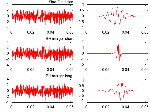
As the HHT is an empirical technique that is not yet supported by a fully independent theoretical basis, we test our approaches through numerical simulations. Throughout this paper we use three test signals to demonstrate our proposed methods (Fig. 1): a Sine-Gaussian at $f_{0}=200$ Hz with Q of 9 ($h_{S\!G}=A\sin(2\pi f_{0}t_{i})\exp(-(2\pi f_{0}(t_{i}-t_{o}))^{2}/2Q)$), spanning 55 msec with 9 oscillations; a numerical simulation of a black hole binary merger (total mass of 20 solar masses ($M_{\odot}$), (hereafter referred to as short BH merger)Baker et al. (2006), which shows strong non-linear frequency modulation from $\sim$300 Hz to $\sim$900 Hz over 5 msec and 3 oscillations; and a 60 $M_{\odot}$ BH merger (hereafter referred to as long BH merger), drifting in frequency from $\sim$100 to $\sim$300 Hz over 20 msec. We place these signals in a time window of 62.5 msec white Gaussian noise, bandpass limited to 1000 Hz at SNR=8, at a sampling frequency of 16384 Hz.

Figure 1: Three test signals at SNR=8 are used in this paper to illustrate our approaches - a Sine-Gaussian at 200 Hz with Q of 9 in the top panels and a numerical simulation of a black hole binary merger (referred to as BH merger, for details see text) in the middle (total mass low, short duration) and bottom (total mass high, long duration) panels. We show the signals (right side), and the signals injected in white Gaussian noise at SNR=8 (left side).

II Detection METHODS

II.1 Detection statistics and Bayesian blocks

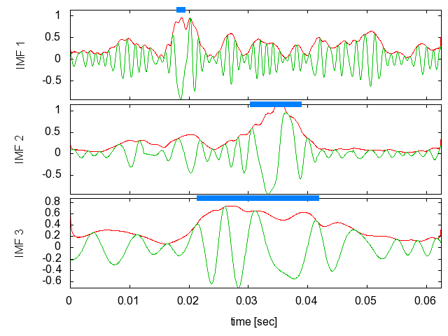
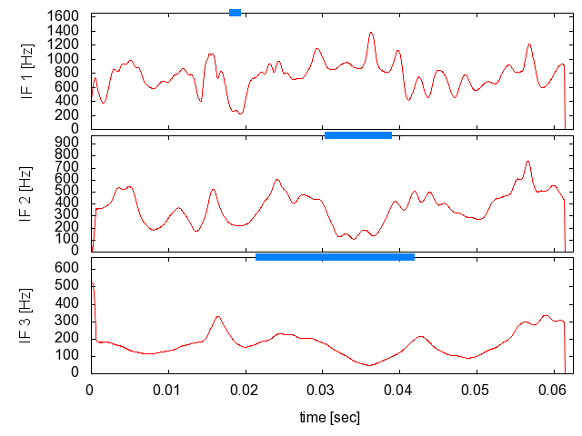
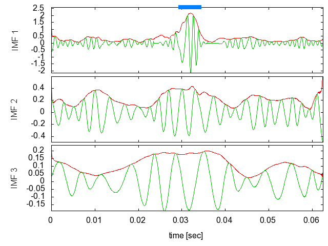
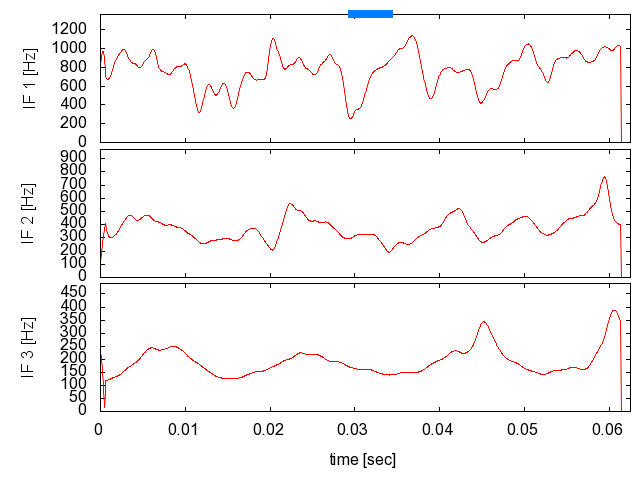
EMD decomposes stationary white noise data in the absence of signals according to a dyadic filter bank, where the mean frequency of the IFs in $n$th-IMF is $\propto f_{s}/2n+1$ where $f_{s}$ is the data sampling rate Flandrin et al. (2004); Huang and Shen (2005); Wu and Huang (2004). The HHT power spectrum, derived by plotting the instantaneous power IP ( = IA²) per frequency interval, shows a uniform distribution of power over frequencies Wu and Huang (2004), indicating that the decomposition preserves the flat frequency content of white noise. This allows us to formulate an HHT detection strategy for a signal in noise, by searching for a temporal region of excess power which is statistically distinguishable from the case of noise with no signal. We show in Fig. 2 the EMD decomposition of the three test signals, where the IA is seen as an upper envelope to the IMFs. Regions of excess power can clearly be seen.

Sine-Gaussian

BH merger short

BH merger long

Figure 2: The IMF, IA (upper envelope of the IMF) and IF of an EMD decomposition of our three test signals. The presence of a signal is indicated by an elevated power level. We observe Bayesian blocking to identify equi-statistical regions of the IP, with regions in which the mean and the standard deviation of the IP is significantly different compared to a noise-only test scenario indicated in blue at the top axis of each panel.

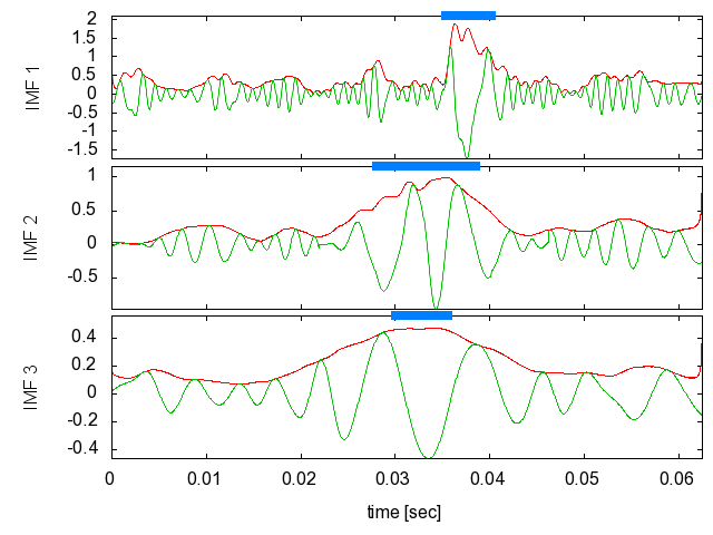
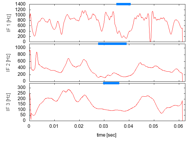
The excess power in a time series can be quantified in a number of different ways, each of which provides a statistic which may be compared to a threshold to indicate a detection. We tested several quantities for the exact formulation of the statistic: 1) the sum over all the IAs in every IMF (sumPow), 2) the maximum IA as seen across all IMFs (maxPow), 3) identifying temporal regions in IA which are significantly above noise levels in their mean value, and deriving the mean over these regions (stat1), 4) identifying temporal regions in IA which are significantly above noise levels in their mean value, and deriving the sum over these regions (stat2), 5) combining stat1 and stat2 by adding the normalized statistic values for each trial (stat1+2). We note that the latter three statistics are adaptive, and require the use of a technique known as Bayesian blocks Scargle (1998); McNabb et al. (2004).

Bayesian blocks determine temporal regions of excess power based on the Bayesian analysis of the relative probability of two different hypotheses. The first hypothesis ($M_{1}$) is that a data segment $X_{n}$ is drawn from a distribution characterized by a single mean $(\mu)$ and variance $(\sigma^{2})$ and the second, that the segment $X_{n}$ consists of two continuous and adjacent sub-segments each drawn from a distribution characterized by a different $\mu$ and/or $\sigma^{2}$, as separated by a discrete “change point” in the individual statistics. The probability that a given data set is drawn from a normal distribution with unknown $\mu$ and $\sigma^{2}$ is equal to:

$P(X_{n}|M_{1})=\int d\sigma\int d\mu(2\pi\sigma^{2})^{-\frac{N}{2}}P(\mu,\sigma)\Pi_{k=0}^{N-1}e^{-\frac{(x_{k}-\mu)}{2\sigma^{2}}}$,

where $P(\mu,\sigma)$ is the a priori probability that the mean and the variance takes on a specific value. Data blocks are defined by finding the temporal start and end point of a deviation in $\mu$ or $\sigma$ (in which several change points in one data stretch are found by iteratively applying the algorithm to each data stretch to the left and right of a just found change point). Temporal regions of excess power are defined by finding blocks with significantly elevated $\mu$ or $\sigma^{2}$. We refer to McNabb et al. (2004) for details. The identification of the Bayesian blocks that indicate regions of $4\sigma$-excess power in our test signals is shown in Fig. 2 as the blue bars at the top of the panels.

II.2 Efficiency Curves

Figure 3: We show the histograms of the detection statistic value stat1+2 and maxPow over $10^{6}$ trials (noise only) and $10^{4}$ trials (signal injections) for the short BH merger. As stat1+2 implements a threshhold in IA we find a significant fraction of the detection statistic equal to zero, as indicated at the left of the plot. The threshhold for a FAR $10^{-2}$ Hz and $10^{-3}$ Hz is indicated as black vertical line. Detection efficiency is defined as fraction of triggers above threshold for given FAR. (For details see text).

Figure 4: The efficiency curves for our three test signals. We show FAR of $10^{-2}$ Hz (red), $10^{-3}$ Hz (green) and $10^{-4}$ Hz (blue), and display detection efficiency vs SNR. Based on these plots, we choose stat1+2 as our detection statistic.

Figure 5: Estimation of the maximum frequency in our three test signals (SNR 8). The generation of a Fourier power spectrum over the boundaries of the triggered blocks within the lowest IMF allows an estimate of the signal maximum frequency. The estimate is inexact (high) due to time-frequency uncertainty of the Fourier analysis. By restricting the analyzed region to the detected blocks within IMFs we eliminate a significant fraction of the noise background, allowing a cleaner determination of the maximum frequency.

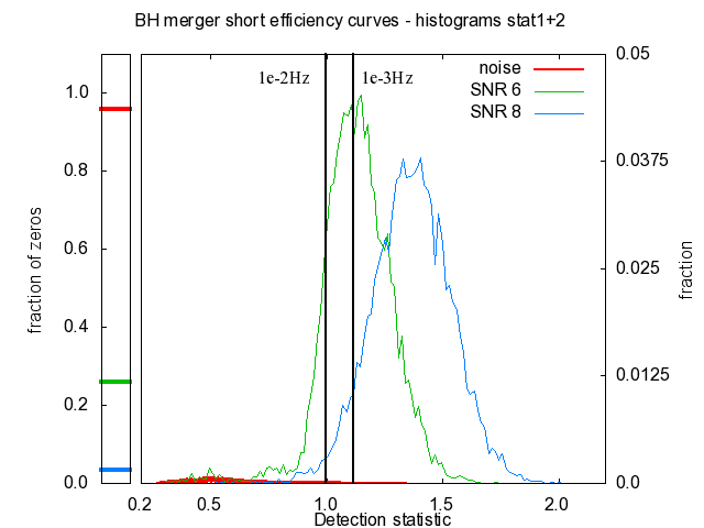
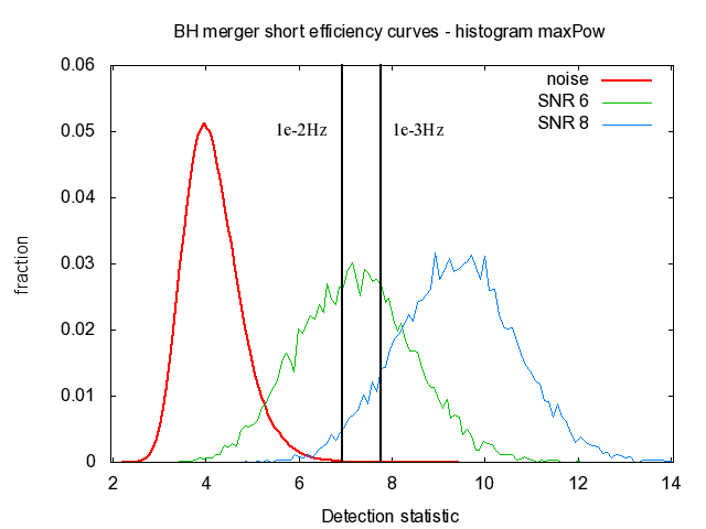
To judge the usefulness of the various statistics to identify signals in noise, we use a Monte Carlo approach to generate detection efficiency curves as followsHelstrom (1968); Metz (1978). After choosing the detection statistic, a set of trials are performed on noise without a signal to track the rate of noise detections, or false alarm rate (FAR), which may be caused by extrinsic uncertainties or statistical fluctuations of the noise power at any given instant. A threshold is set to yield the FAR at a low value, typically $10^{-2}$ Hz to $10^{-3}$ Hz (for our trial time window of 62.5 msec). Next a signal of given SNR is added to a white noise time series. The HHT decomposition is run and the extracted value of the detection statistic is compared to the threshold to determine whether a detection was made. This is repeated for a large number of trials to examine the efficiency of signal detection at a given SNR and FAR. We show in Fig. 3 examples of the histograms for stat1 and maxPow detection statistics with $10^{6}$ noise-only trials and $10^{4}$ signal injection trials per given SNR for the short BH merger. We additionally show the noise only distribution and display the specific FAR of $10^{-2}$ Hz and $10^{-3}$ Hz, corresponding to 625 and 63 false alarms per million trials respectively. We note that the adaptive detection statistics stat1, stat2 and stat1+2 use a $4\sigma$ IA threshold in each decomposed IMF to identify a block, which is also required to consist of at least 4 data points; these conditions limit noise fluctuations from exceeding the detection threshold. Thus for stat1+2 $96\%$ percent of noise detection statistic values are zero, as indicated in Fig. 3. In contrast, the added amplitude of signals results in an increased detection efficiency so that only $25\%$ of the detection statistic values are zero at SNR 6 and $3\%$ are zero at SNR 8. The detection statistic maxPow and sumPow do not use a threshold in IA, thus their histograms of the statistics of signal and noise do not show zeros and are Gaussian in shape.

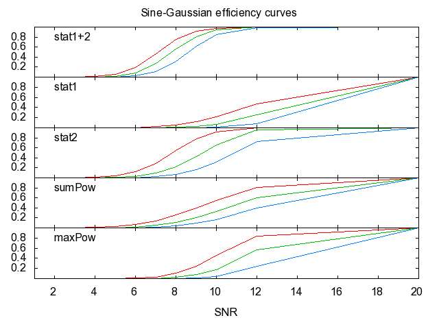
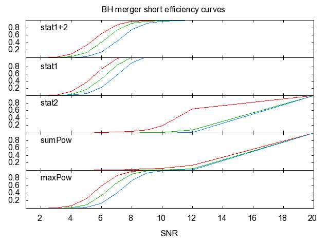
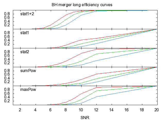
We display in Fig. 4 the efficiency curves for all five detection statistics as applied to the three test signals, where we plot detection efficiency for the three test signals vs. SNR, with FAR of $10^{-2}$ Hz, $10^{-3}$ Hz and $10^{-4}$ Hz. We draw a number of conclusions from these plots. In general we find that shorter signals at a fixed SNR show a higher detection efficiency, as they show larger $I\!A/\sigma_{n}$, as discussed earlier. We also find that the adaptive statistics stat1, stat2 and stat1+2 perform better than maxPow and sumPow in most cases, due to the efficiency of the Bayesian blocks in identifying signals. We find that stat1 tends to trigger on excess power in short regions, while stat2 is more efficient for excess power over longer intervals, assuming the same amount of total added power is placed in either short or long regions respectively; thus the combined statistic stat1+2 appears to be efficient for the range of our test signals. We identify outliers from extrinsic HHT uncertainties yielding a $4\sigma$ level IA increase over a given region to primarily contribute to false alarms in stat1, stat2, and stat1+2. Finally, we note that all three signals are best detected at the 50$\%$ efficiency level with stat1+2 for all false alarm rates. We therefore choose stat1+2 as detection statistic for the remainder of the paper.

II.3 Additional information from Bayesian blocks

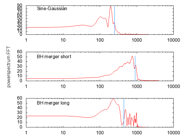
Additional information about the signal can be obtained by analyzing the detected blocks: the start and end times of the event can be derived by looking at the outermost edges of all the triggered blocks over the IMFs, and the SNR of the detected event may be estimated by summing over the amplitude of the triggered blocks and comparing to the standard deviation of the noise. Finally, the maximum frequency of the signal, a very important quantity in this analysis, may be obtained by examining the Fourier power spectrum of the shortest data stretch that includes all the triggered blocks of the lowest IMF. We show below that the signal can be greatly clarified in the characterization stage by applying a low-pass filter based on this maximum frequency, which removes noise in the time series that is outside the bandwidth of the signal evolution. We illustrate the derivation of the maximum frequencies in Fig. 5, where we have generated the power spectra of the detected blocks for each test signal. We find that an effective way to separate the upper edge of the power spectrum from the noise background is to identify the first inflection point after the spectrum peak and round up to the next highest multiple of 50 Hz in frequency. We note that restricting the analyzed region to the detected blocks eliminates a significant fraction of the noise background (roughly the ratio of length of the signal to the length of the time window), allowing a cleaner determination of the maximum frequency.

III Characterization methods

With the identification of a region of excess power that indicates a signal, we consider methods to accurately characterize the signal including its frequency evolution in time. With these methods we seek to reduce extrinsic and intrinsic uncertainties, and also to estimate the remaining uncertainty. We further look into the special case of very low SNR ($<$5) signal characterizations.

III.1 Reduction of extrinsic and intrinsic uncertainty

Figure 6: The use of a zero-phase filter specified in the detection stage is used to remove noise from the data above the maximum frequency of the event. Here we show the three test signals before (first panel of each plot) and after the filtering (second panel of each plot). The third panel shows the result of applying EEMD to the filtered waveform, which now yields the signal in the first IMF, as opposed to the multiple IMFs of 2. Comparison of this result with the signal waveform (in blue) shows the effectiveness of the filtering method. Finally, in the forth panel we show the IFs derived from IMF1, which are considerably more accurate than those of Fig. 2.

Figure 7: The IF of the first IMF of the test signals as derived either by a 3-point differentiation rule or the least squares velocity filter (LSVF), here using a 20-point averaging. The 3-point estimate experiences fluctuations that are non-physical, reaching values larger than 1000 Hz in noisy regions although the data bandwidth is 1000 Hz. The LSVF reduces the largest fluctuations and singularities.

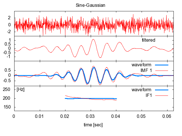
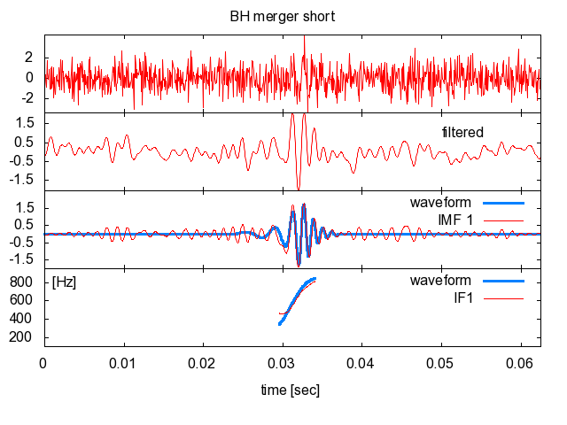
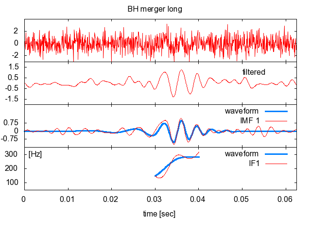
The most effective method to suppress extrinsic uncertainties in the decomposition of the time series into its IMFs was the implementation of an aggressive zero-phase FIR low-pass filter techniqueSmith (2009), removing noise with frequency content above the maximum frequency of the signal. We illustrate this procedure in Fig. 6 using the test signals. The application of a filter with low-pass frequency close to the maximum frequency of the waveform removes the need for decomposition of the data into multiple IMFs before the signal is encountered, and reduces the associated extrinsic uncertainties caused by numerous envelope generations, and their possible over-/undershoot. Using the filtering, the very first EMD decomposition directly targets the frequency scales of the signal. Furthermore, the filter suppresses fluctuating noise which can cause different parts of the signal to appear in different IMFs. The filter needs to satisfy several requirements: a) it must be zero-phase so that the slope of the signal is not altered by phase dispersion; b) it should have a very sharp transition from the pass band (below the filter frequency) to the stop band (above the filter frequency) to allow it to remove frequency content close to the signal; c) it should suppress ringing in the pass band and stop band; d) the filter frequency should be as close as possible to the maximum frequency of the signal to be most effective in filtering noise (we estimate that the filter cut off frequency should not be closer than 50 Hz to the intrinsic maximum frequency of the signal to avoid distorting the signal waveform.) The filter cut-off frequency can be found adaptively, as mentioned above, by generating a Fourier spectrum of the signal region of the lowest IMF identified by the Bayesian blocks. This estimate yields 250 Hz, 900 Hz and 450 Hz as filter frequency for the Sine-Gaussian, the short BH merger and the long BH merger respectively, as shown in Fig. 5.

After application of the zero-phase filtering, envelope over/undershoot in the remaining EMD decomposition can be reduced with ensemble EMD (EEMD,Wu and Huang (2008)) methods. In this technique ensembles of data are produced by injecting small, random distributions of Gaussian white noise into the original data stream. EMD is then performed on each ensemble member, with the result that each member suffers a perturbation of the position of local maxima and minima and thus a slightly different envelope fitting. The error propagation related to any member of the ensemble tends to be attenuated once the ensembles are averaged, yielding a better measure of the signal compared to one EMD run alone. We average over 20 ensemble members, and inject white Gaussian noise at 10 percent of the original time series noise standard deviation.

To demonstrate the effectiveness of the zero-phase filtering, we compare in Fig. 6 the true IF evolution of the test signals with the decomposed IFs version. The panels of the plots, from top to bottom, show: 1) the time series of the signal in noise with SNR=8; 2) the time series obtained from the application of the zero-phase filter with filter frequency found as described above; 3) the first IMF obtained from the application of EEMD to the filtered time series; 4) the IF obtained from the first IMF. In panels 3 and 4, the blue trace shows the first IMF and IF of the actual signal without noise. We find the decomposed IF to closely approximate the true IF in all three test cases: where the filtered signal amplitude is largest the agreement is $\Delta f/f\leq 0.1$, while the error becomes larger at the signal boundaries where the amplitude becomes comparable to the noise. These errors represent the combination of remaining intrinsic and extrinsic uncertainties, and are quantified in the next section. The improvement of the IF evolution as found in the final characterization stage relative to the detection stage (Fig. 2) is apparent: the Sine-Gaussian now appears well resolved in its (flat) IF evolution, and the long BH merger shows significantly less oscillatory behaviour in the IF after filtering. The short BH merger IF did not change significantly as the signal showed sufficient $I\!A/\sigma$ contrast to provide an accurate derivation of the IF in the detection stage, and the data cut off frequency of 1000 Hz is close to the estimated signal maximum frequency of 900 Hz.

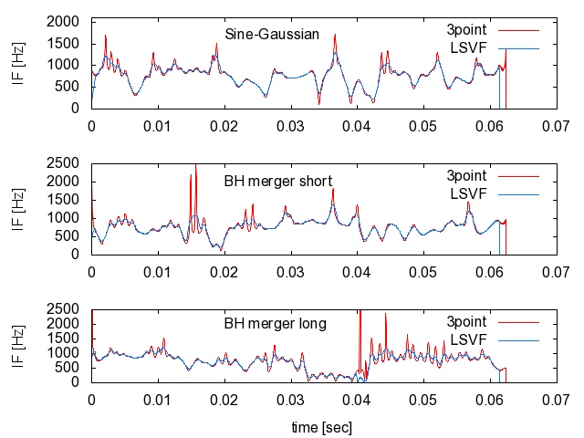
Remaining uncertainties in the IF determination can take the form of singularities and/or oscillations outside the physical IF range which are caused by noise-induced spurious oscillations in the phase. These oscillations may be controlled by implementing a least squares velocity filter (LSVF), which provides a 2nd order polynomial fit to a specified number of points of the IFs, thereby averaging over sharp IF fluctuations. Frequencies in IMFn that are much greater or much less than the range implied in the dyadic structure $\propto f\!s/2n+1$ will be attenuated with this technique. In our examples we use a filter of order 20 to derive the frequency from the phase, which smooths the shape of 20 consecutive data points to derive one IF value. This is illustrated in Fig. 7.

III.2 Estimation of uncertainties

Figure 8: Estimation of the time-frequency-uncertainty for the test signals with the Sine-Gaussian in the upper panel and the short and long black hole mergers in the lower two panels. The uncertainty is indicated by an envelope (white lines) about the time-frequency trace of the signal (colored trace)

An analytical estimate of the uncertainty of the IMF, IA or IF of a decomposed signal at low SNR is difficult to establish, due to the empirical nature of the HHT decomposition. But it is possible to define the relative uncertainty of the individual decomposition by looking at its variance with respect to a perturbation of the time series. As described above, we use the EEMD averaging process to obtain an accurate measure of the IFs by averaging and smoothing out extrinsic uncertainties. We can also use the EEMD as a tool to determine the uncertainty of the decomposition. Since EEMD injects noise at all frequencies into the data stream, it will alter both the envelope fitting and the signal waveform itself. Thus to quantify the total uncertainty we apply EEMD with an injection of an additional amount of noise equal to the noise level of the data.

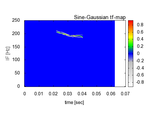
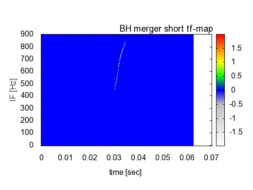
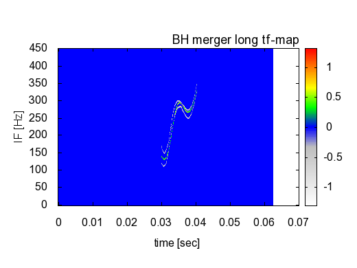
In detail, we create an ensemble consisting of 40 members by summing the time series with different realizations of white Gaussian noise with the same standard deviation of noise found in the data (the noise standard deviation is estimated outside the block boundary which marks the signal region.) We then apply a zero-phase low-pass filter at the maximum frequency of the signal to each member of the ensemble, perform an EMD decomposition and finally derive the IF distribution. This new decomposition is subject to large intrinsic uncertainties as the additional injected noise significantly changes the slope of the waveform, and large extrinsic uncertainties as the EMD envelope fitting is distorted by the altered local maxima which propagates through the iterative process. The 40 members of the ensemble then carry a different IF value at each time; the spread is used to derive a 2$\sigma$ uncertainty envelope. The IF trace derived from the original data lies within the uncertainty envelope, with the width of the envelope displaying the confidence of the IF derivation. In Fig. 8 we show two dimensional time-frequency (tf) maps that plot IF and IA of the three test signals vs. time, with power as color. We find the time-frequency traces to fit inside the uncertainty envelopes, with the uncertainties becoming relatively large where the amplitude to noise ratio becomes small.

III.3 Kernel density estimates and very low SNR signal characterization

Figure 9: The tf-map and the KD-tf map of the Sine-Gaussian at SNR=4 (top panels) and the short BH merger at SNR=3.

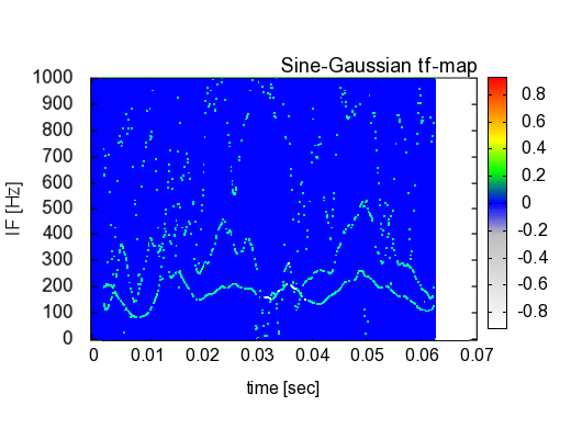
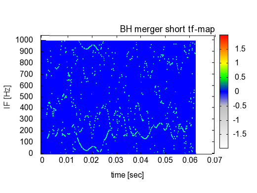
We now consider the case of data analysis on signals at SNR $<$5, in the case of our test signals $I\!A/\sigma$ ratios of less than 0.6. In order to detect these signals the threshold of the detection statistic stat1+2 as described in Sec. II has to be lowered (see Fig. 4). This results in the unavoidable generation of errors: noise bursts can trigger blocks, resulting in poorer overall detection sensitivity as noise enters the detection statistic; the number of false alarms increases; and within the event blocks we find poorer timing estimates and upper frequency estimates for the signal. These errors lead to poor tf map evaluations as the noise may be comparable or stronger in power than the signal, and also noise is not effectively removed from the tf map by considering only triggered blocks.

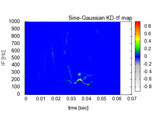
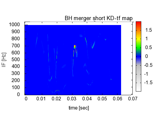
A method to regain signal contrast in SNR$<$5 tf maps is the following. We seek to take advantage of the fact that signal remnants show coherent structure and follow the underlying trend of the true signal in the tf-plane by clustering around its idealized true positions (in absence of noise) with elevated power levels. Noise in comparison is incoherent and scatters over the tf plane with random power levels. Thus signal regions can be identified by locating clustered tf traces with elevated power levels.

We find weighted kernel density estimates on the tf-plane (KD-tf) best suited to highlight signal regions Silverman (1986). The KD-tf starts with the assumption that a signal structure is evident in the data, and that it would, in absence of noise, place a coherent and continuous trace in the tf-plane. We posit this idealistic trace as a probability density distribution, effectively showing no density outside the signal trace and a sharp, peaked probability density within the signal trace where a coherent structure can be found.

We implement an adaptive weighted kernel density estimate to recover this signal probability density. The kernel, $K(t,f)$, is a bi-variate Normal distribution, with dimensions of time and frequency

$$K(t_{i}-t_{j},f_{i}-f_{j})=\frac{1}{2\pi\sigma_{t_{j}}\sigma_{f_{j}}\sqrt{1-\eta_{j}^{2}}}\exp\left[-\frac{z}{2(1-\eta_{j}^{2})}\right]$$ (2)

with

$$z=\frac{\left(t_{i}-t_{j}\right)^{2}}{\sigma_{t_{j}}^{2}}+\frac{\left(f_{i}-f_{j}\right)^{2}}{\sigma_{f_{j}}^{2}}-\frac{2\eta_{j}\left(t_{i}-t_{j}\right)\left(f_{i}-f_{j}\right)}{\sigma_{t_{j}}\sigma_{f_{j}}}$$ (3)

and

$$\eta_{j}=\frac{\sigma_{t_{j},f_{j}}}{\sigma_{t_{j}}\sigma_{f_{j}}}$$ (4)

In the density estimate every point $[t_{j},f_{j}]$ in the tf-plane carries its own kernel, whose standard deviation in both dimensions $\sigma_{t_{j}},\sigma_{f_{j}}$, and correlation $\sigma_{t_{j},f_{j}}$, is estimated adaptively on the basis of the tf-plane population. Intuitively, a point within a sparse population (e.g. incoherent noise scattering) should carry a wide and flat kernel, while points within a coherent clustering of signal remnants should carry a peaked and sharp kernel. This contrast allows the signal to be emphasized relative to the noise. The contrast can be seen most clearly at frequencies near the data sampling rate, and is found by applying EMD to each IF and retaining only the first IMF, which removes all but the highest frequency content in each IF. Scanning each high frequency IF distribution for changes in the standard deviation, and using the Bayesian blocking technique to find the kernel specifics at each point, we find signal remnants and noise sources blocked separately and associated with different mean, correlation and standard deviation. Each point within a block uses the statistics of the block to establish its individual kernel. The final estimate is built according to

$$KD\!-\!tf_{i}=\sum_{j}I\!P_{j}^{2}K(t_{i}-t_{j},f_{i}-f_{j})$$ (5)

where we weigh the power of the signal trace in quadratic terms to balance contributions from clustering (as contained in the Kernel) with power.

We demonstrate the advantages of the KD-tf for low SNR in Fig. 9. We show two examples, the Sine-Gaussian at SNR=4 and the short BH merger at SNR=3. In both cases the estimation of the upper frequency of the signal was not possible because of the low SNR, and thus filtering was not used, leading to relatively large extrinsic uncertainties. We see that the KD-tf maps help to better define the signal remnants and improve the signal to noise contrast ratio. We find the Sine-Gaussian to oscillate around its center frequency, and the short BH merger to only reveal the very peaked part of its waveform, the merger/ring-down transition at $\sim$870 Hz. We estimate that KD-tf techniques are applicable only if the maximum $I\!A/\sigma$ ratio is larger than 0.3.

IV Discussion

We presented in this paper methods to enable the HHT to efficiently detect and accurately characterize signals in the low SNR ($<$20) regime. Since the overall power contained in the data is roughly preserved by the HHT decomposition, we were able to construct strategies to search for excess power to find a signal in comparison to a noise only decomposition. The concept of Bayesian blocking was introduced to adaptively locate regions of excess power, and therefore to localize and analyze the signal while also gaining sensitivity by limiting noise contributions to the detection statistic. We derived efficiency curves which showed that our black hole merger and Sine-Gaussian test signals could be detected with better than 50% efficiency at SNR $<$8 with FAR = $10^{-3}$ Hz. We then considered measures to accurately derive the IF at low SNR. We proposed zero-phase FIR low-pass filters and LSVF filters to reduce the amount of extrinsic IF uncertainties, and KD-tf mappings to limit intrinsic IF uncertainties. A measure of the uncertainty or reliability of the decomposition was obtained by testing the dependence of the extracted signal waveform on increased extrinsic and intrinsic IF uncertainties.

One direction for future research is the estimation of the upper frequency of the event. We found FFT methods to overestimate an upper limit to the signal frequency because of inherent FFT time-frequency uncertainty. Also, if the signal maximum frequency shows a strong gradient the FFT estimate becomes even more spread out, resulting in ineffective subsequent FIR filtering. A possible approach to obtain a more accurate measure is to assess the maximum frequency with the IF and the IA, but this is more noise sensitive than the FFT, especially if the signal shows its largest frequency at low amplitude. A combination of both approaches might be optimal.

Finally, we have investigated other adaptive decomposition methods to compare their extrinsic error generation with those of EMD. (ITDFrei and Osorio (2007), sawtooth transformLu (2007), fastEMDLu (2008)). We find that the EMD has a significant advantage due to the way it handles waveform inflections, which can either be caused by multiple oscillations needing further decomposition, or by a frequency modulation that is a true physical property of the underlying waveform. EMD is able to effectively differentiate between these, while the ITD and the sawtooth transform methods do not, and the fastEMD incorrectly decomposes all inflections into multiple oscillations in distinct modes. We note that only with a proper decomposition can our proposed additional filters help significantly in the process of detecting and characterizing the signal.