Nuclear quantum effects in solids using a colored-noise thermostat

Abstract

We present a method, based on a non-Markovian Langevin equation, to include quantum corrections to the classical dynamics of ions in a quasi-harmonic system. By properly fitting the correlation function of the noise, one can vary the fluctuations in positions and momenta as a function of the vibrational frequency, and fit them so as to reproduce the quantum-mechanical behavior, with minimal a priori knowledge of the details of the system. We discuss the application of the thermostat to diamond and to ice Ih. We find that results in agreement with path-integral molecular dynamics can be obtained using only a fraction of the computational effort.

Nuclear quantum effects are extremely important in many condensed-phase systems. For instance, zero-point fluctuations affect static correlations, and energy quantization causes deviations from the classical value of the specific heat at low temperatures. A quantum treatment of the ionic degrees of freedom is mandatory to capture such effects, which are particularly important when light atoms or stiff vibrational modes are present. However, including quantum effects is computationally demanding, even if one is interested only in equilibrium properties, as is the case here. For this reason, the nuclei in molecular simulations are often treated classically, even when the electronic degrees of freedom are accounted for quantum-mechanically Marx and Hutter (2000).

When exchange-symmetry effects are not relevant, the method of choice for studying equilibrium expectation values is path-integrals molecular dynamics (PIMD) Ceperley (1995); Marx et al. (1999). However, this comes at a high computational cost, since many replicas of the system need to be simulated in parallel. Approximate but less expensive methods such as Feynman-Hibbs effective potentials Feynman-Hibbs have also been used, as well as semiclassical approaches to treat zero-point energy (ZPE) Semiclassic . Their range of validity is limited to weak quantum behavior, and to cases where the Hessian of the potential is available and cheap to compute. The interest in methods to introduce quantum effects in classical trajectories is thus still very high, see e.g. Ref. recent for recent applications.

In a recent work Ceriotti et al. (2009) we have demonstrated that a generalized, linear Langevin equation with colored noise can be used to obtain a highly tunable thermostat for constant-temperature molecular dynamics. In this Letter we will show that, by suitably extending this idea, it is possible to modify Hamilton’s equations so as to introduce the quantum-mechanical effects. Furthermore, this comes with only a negligible increase in computational effort with respect to traditional classical simulations, and requires a minimal prior knowledge of the properties of the system. The idea can be traced back to the semiclassical approximation to the quantum Langevin equation gle , which has been used to model quantum systems in contact with a quantum harmonic bath. A similar idea has been recently used by Buyukdagli et. al Buyukdagli et al. (2008), in order to compute quantum specific heat in harmonic systems. However, Buyukdagli’s scheme is only qualitatively correct even for a harmonic oscillator, and neglects ZPE completely. In this Letter we propose a more general approach, which allows one to obtain high accuracy in reproducing quantum specific heats, and also tackles the more challenging task of introducing zero-point motion effects. This is achieved by effectively and automatically enforcing the quantum position and momentum distributions. Our method gives excellent results in systems with limited anharmonic coupling, and is ideal for treating quantum effects in solids.

Let us first consider a harmonic oscillator which is evolved in time according to a generalized Langevin equation. This equation can be written in a Markovian form by suitably extending the state vector Marchesoni and Grigolini (1983); Gardiner (2003); Ceriotti et al. (2009). For each degree of freedom, a set of $n$ additional momenta $s_{i}$ are introduced, which complement the position $q$ and the physical momentum $p$. The value of $n$ depends on the structure of the memory kernel for the generalized Langevin equation and, in our experience, a choice between $4$ and $12$ allows sufficient flexibility. For simplicity, we assume mass-scaled coordinates, $q\leftarrow q\sqrt{m}$ and $p\leftarrow p/\sqrt{m}$. We introduce a compact convention to represent matrices acting on the state vector $\left(q,p,\mathbf{s}\right)^{T}$:

$$\begin{array}[]{ccccc}&q&p&\mathbf{s}&\rule{0.0pt}{12.0pt}\\ \cline{2-4}\cr\lx@intercol\hfil q\hfil\lx@intercol\vrule\lx@intercol&a_{qq}&a_{qp}&\lx@intercol\hfil\mathbf{a}_{q}^{T}\hfil\lx@intercol\vrule\lx@intercol&\rule{0.0pt}{12.0pt}\\ \cline{3-4}\cr\lx@intercol\hfil p\hfil\lx@intercol\vrule\lx@intercol&\lx@intercol\hfil\bar{a}_{qp}\hfil\lx@intercol\vrule\lx@intercol&a_{pp}&\lx@intercol\hfil\mathbf{a}_{p}^{T}\hfil\lx@intercol\vrule\lx@intercol&\rule{0.0pt}{12.0pt}\\ \cline{4-4}\cr\lx@intercol\hfil\mathbf{s}\hfil\lx@intercol\vrule\lx@intercol&\lx@intercol\hfil\bar{\mathbf{a}}_{q}\hfil\lx@intercol\vrule\lx@intercol&\lx@intercol\hfil\bar{\mathbf{a}}_{p}\hfil\lx@intercol\vrule\lx@intercol&\lx@intercol\hfil\mathbf{A}\hfil\lx@intercol\vrule\lx@intercol&\rule{0.0pt}{12.0pt}\\ \cline{2-4}\cr\end{array}\begin{array}[]{cc}\rule{0.0pt}{12.0pt}\\ \rule{0.0pt}{12.0pt}\\ \left.\rule{0.0pt}{12.0pt}\right\}\!\mathbf{A}_{p}\\ \end{array}\begin{array}[]{cc}\rule{0.0pt}{12.0pt}\\ \left.\rule{0.0pt}{20.0pt}\right\}\!\mathbf{A}_{qp}\end{array}$$ (1)

Thus, a matrix without subscript acts on the subspace of additional momenta only. The $p$ and $qp$ subscripts denote matrices which also act on the $p$ and on the $(q,p)$ respectively. The Markovian form for the generalized Langevin equation reads

$$\left(\begin{array}[]{c}\dot{q}\\ \dot{p}\\ \dot{\mathbf{s}}\end{array}\right)=-\left(\begin{array}[]{ccc}0&-1&\mathbf{0}\\ \omega^{2}&a_{pp}&\mathbf{a}_{p}^{T}\\ \mathbf{0}&\bar{\mathbf{a}}_{p}&\mathbf{A}\end{array}\right)\left(\begin{array}[]{c}q\\ p\\ \mathbf{s}\end{array}\right)+\left(\begin{array}[]{ccc}0&0&\mathbf{0}\\ 0&\lx@intercol\hfil\hbox{\multirowsetup$\mathbf{B}_{p}$}\hfil\lx@intercol\\ \mathbf{0}&&\\ \end{array}\right)\left(\begin{array}[]{c}0\\ \hbox{\multirowsetup$\boldsymbol{\xi}$}\\ \\ \end{array}\right)$$ (2)

where $\boldsymbol{\xi}$ is a vector of $n+1$ uncorrelated gaussian random numbers. Equation (2) has been chosen as the most general linear stochastic equation where the position $q$ is not coupled with the noise nor with the $s_{i}$. This form allows for an easier generalization to the anharmonic case. The static covariance matrix $\mathbf{C}_{qp}$ can be obtained by solving the matrix equation Zwanzig (2001); Gardiner (2003)

$$\mathbf{A}_{qp}\mathbf{C}_{qp}+\mathbf{C}_{qp}\mathbf{A}_{qp}^{T}=\mathbf{B}_{qp}\mathbf{B}_{qp}^{T}$$ (3)

In Ref. Ceriotti et al. (2009) we have chosen $\mathbf{B}_{p}$ so as to obtain $\mathbf{C}_{p}=k_{B}T$ ($c_{qq}=k_{B}T/\omega^{2}$, in our units), which corresponds to enforcing detailed balance. In a quantum oscillator at finite temperature the distribution of position and momentum is still Gaussian, but its variance has a nontrivial dependence on $\omega$, i.e. $\left<p^{2}\right>=\omega^{2}\left<q^{2}\right>=\frac{\hbar\omega}{2}\coth\frac{\hbar\omega}{2k_{B}T}$. We can therefore perform a fitting procedure, tuning $\mathbf{B}_{p}$ and $\mathbf{A}_{p}$ so that the $\omega$-dependence of $c_{qq}=\left<q^{2}\right>/\omega^{2}$ and $c_{pp}=\left<p^{2}\right>$ reproduces closely the exact quantum fluctuations. The fitting procedure is not trivial, and will be discussed elsewhere. Once a set of parameters has been found which guarantees a good fit over a certain frequency range $\left(\omega_{\text{min}},\omega_{\text{max}}\right)$, the thermostat automatically enforces the correct quantum fluctuations for any system whose typical vibrations fall within this range. Tipically, an error below a few percents can be obtained over a frequency range spanning several orders of magnitude. In the harmonic limit, the momentum and position distributions computed using our thermostat sample the quantum distributions within the accuracy of the fit. Furthermore, it is easy to show that the averages of any local operator which depends separately on positions or momenta are also correctly computed.

In the general, anharmonic case, the coupling between position and momentum is nonlinear. Therefore, one needs to use a finite time step; in particular, one proceeds by first integrating the $\left(p,\mathbf{s}\right)$ variables, which can be evolved using the exact finite-time propagator built from $\mathbf{A}_{p}$ and $\mathbf{B}_{p}$, and then updating $q$ and $p$ by integrating Hamilton’s equations Bussi and Parrinello (2007).

Figure 1: (color online) Mean total ($\left<E\right>$), potential ($\left<V\right>$) and kinetic ($\left<K\right>$) energy for a proton in the external potential of Eq. (4) as a function of $\omega$, for $k=1$ Å^-1 and $T=100$ K. In the inset, the Fourier transform of the momentum distribution is reported for the fully quantum, classical and colored-noise thermostat simulations at $\omega=200$ cm^-1. Dashed black lines correspond to the exact quantum solution, the dark (red) series are results from present work, using a set of parameters fitted over a frequency range from $2$ to $2000$ cm^-1. Light (blue) lines correspond to the classical expectation values.

As a first example, we apply this method to a one-dimensional, anharmonic potential of the form

$$V\left(x\right)=\frac{\omega^{2}}{2m}x^{2}\frac{1-e^{-kx}}{kx}$$ (4)

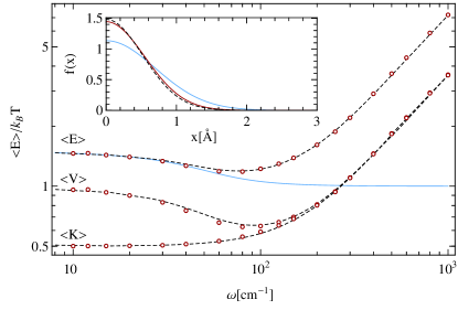
For a fixed value of $k$ and temperature $T$, this potential allows one to explore a range of behaviors that goes from the highly anharmonic, classical limit at $\omega\rightarrow 0$ to a quantum, harmonic regime at high $\omega$. In Figure 1 we compare the exact, quantum solution with the averages obtained using our colored-noise thermostat. There is a remarkably good quantitative agreement not only in the asymptotic $\omega\rightarrow 0$ and $\omega\rightarrow\infty$ limits, but also in the intermediate region, where quantum-mechanical and anharmonic effects are significant, suggesting that both can be captured, albeit not fully. Also the momentum distribution (shown in the inset) is in good agreement with its quantum-mechanical counterpart. This is particularly appealing, since conventional PIMD can only sample positions, and one must introduce special procedures to sample momenta as well Ceperley and Pollock (1986); Morrone et al. (2007); Morrone and Car (2008).

We now move on to more complex and realistic applications. As we have already discussed Ceriotti et al. (2009), if one applies a separate thermostat to each degree of freedom, the multidimensional harmonic problem can still be solved analytically, by projecting the dynamics onto the normal modes. One would then expect independent phonons to thermalize at different effective classical temperatures according to the target $c_{qq}\left(\omega\right)$ and $c_{pp}\left(\omega\right)$ relations, provided that the response to the thermostat is faster than the anharmonic coupling between different phonons. Heuristically, one would expect that the error on the energy of a phonon of frequency $\omega_{i}$ would grow with the coupling time $\tau_{H}(\omega_{i})$, as defined in Ref. Ceriotti et al. (2009), and with the largest difference in target energy, $\Delta E=c_{pp}(\omega_{\text{max}})-c_{pp}(\omega_{\text{min}})$. Any such error should instead decrease with the classical lifetime of the phonon $\tau_{L}(\omega_{i})$, which gauges the internal energy transfer to other vibrational modes. This effect can be reduced to a great extent by modifying the fit such that not only are the quantum distributions reproduced, but also the correlation time $\tau_{H}$ is made as small as possible.

Figure 2: (color online) Lattice parameter of diamond as a function of temperature, computed by isothermal-isobaric runs at atmospheric pressure Hoover (1985). Black dashed lines correspond to PIMD results from Ref. Herrero and Ramírez (2000), and red circles to averages computed from runs using our properly fitted colored-noise thermostat. In inset (a) the average kinetic temperature $T^{\star}$, projected on a few selected normal modes, is plotted for three target temperatures (from top to bottom, $1000$ K, $500$ K and $200$ K) as a function of the mode frequency. The continuous lines are the expected quantum $T^{\star}\left(\omega\right)$ curves. In the inset (b) we compare the total internal energy (kinetic plus potential) as computed with PIMD (black dashed line, Ref. Herrero and Ramírez (2000)) and with colored-noise thermostat fitted to the quantum $E\left(\omega\right)$, with (red circles) and without (gray lozenges) ZPE. The latter (gray) points have been aligned to the PIMD results at $T\rightarrow 0$.

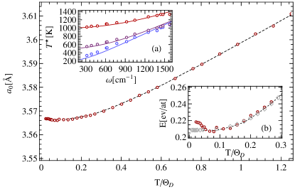
In order to assess the accuracy of this approach, we first study diamond, an archetypical quasi-harmonic system. We used the Tersoff classical potential Smith et al. (2006); Tersoff (1989), for which accurate PIMD results have been reported Herrero and Ramírez (2000). In Figure 2 we compare observables computed with PIMD and with our colored-noise thermostat. The correlated Langevin dynamics is able to reproduce quantitatively the quantum effects on the thermal expansion and on specific heat down to $T\approx 0.1\Theta_{D}$. Only at lower temperatures do we start observing significant discrepancies.

To understand the reason for this breakdown, it is instructive to look at the kinetic temperature $T^{\star}$ of the different phonons [inset (a)]. This is a powerful probe of the accuracy of the method, which can be performed whenever a normal-modes analysis is meaningful. In this case, the normal-modes analysis shows that, in the extremely quantum regime for $T<0.1\Theta_{D}$, the thermostat fails to counterbalance the phonon-phonon coupling due to anharmonicities. Because of this internal coupling, energy flows from the stiff modes (which thermalize at a lower temperature than expected) to the slow ones (which turn out to be hotter than desired). A large energy difference $\Delta E\approx\hbar\left(\omega_{\text{max}}-\omega_{\text{min}}\right)/2$ must be maintained between fast and slow modes. Moreover, because of ZPE, the motion of the ions is not limited to the harmonic region of the potential energy surface. This leads to higher anharmonic coupling and eventually to shorter phonon lifetimes. This explanation is supported by the results shown in inset (b). Here we performed the fit by considering an energy-versus-frequency relation which excludes the zero-point contribution, as done in Ref. Buyukdagli et al. (2008). The agreement with PIMD energies is now virtually perfect, since high-frequency modes are basically frozen and normal modes are almost perfectly decoupled, so that internal energy transfer becomes negligible. However, if one is interested in quasi-harmonic effects, or simply in observables which are functions of the atomic coordinates or velocities, neglecting ZPE would mean sampling an unphysically cold system, where stiff modes are completely frozen. Some examples of such observables are the Debye-Waller factor, radial distribution functions and momentum distributions.

Figure 3: (color online) Radial distribution functions for ice at $T=220$ K. Black, dashed line corresponds to the PIMD results of Hernandez et al. de la Peña et al. (2005), dark (red) and light (blue) series to colored-noise and purely classical runs, respectively. Runs have been performed in isothermal ensemble for a box of 360 water molecules at experimental density Hayward and Reimers (1997), and are $125$ ps-long. In inset (a), we show the experimental proton momentum distribution for ice at $269$ K (black dashed line) Reiter et al. (2004), and corresponding distribution as computed from a classical (blue line) and colored-noise (red line) simulation using a flexible TIP4P-like potential Habershon et al. at the rescaled temperature ($247$ K, i.e. 4K below the quantum melting point of the potential).

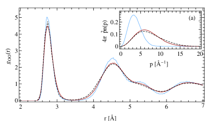
To demonstrate the ability of our method to compute structural properties, we have performed simulations on a TIP4P Jorgensen et al. (1983) model of ice Ih at $220$ K, which poses the additional challenge of showing larger anharmonicity than diamond. In Figure 3 we show the radial distribution function $g_{OO}$ obtained using a classical simulation and our scheme, taking as a reference literature PIMD results de la Peña et al. (2005). The agreement is very good, and the peak broadening is correctly and quantitatively predicted. Fitting the thermostat removing ZPE as in Buyukdagli et al. (2008) leads to an unphysical reduction of the width of the peaks, which are much narrower than for the classical simulation.

We also performed similar calculations using a related flexible water forcefield Habershon et al. , in order to asses the accuracy in a system with an extreme spread of vibrational frequencies. Results are in good qualitative agreement with rigid-water ones, but we cannot perform a quantitative comparison in the lack of PIMD results for flexible water. This agreement demonstrates that a large $\Delta E$ is not a problem, provided that phonon-phonon coupling is weak. For this model we also computed the proton-momentum distribution (see inset of Figure 3). A quantitative comparison with experiment is difficult because of the limitations of the model potential, which makes it difficult to discuss the origins of the discrepancies. For example, the simulation has to be performed $~{}20$ K below the experimental temperature, because of the dicrepancy in the melting temperature. That said, the improvement over the purely classical results is impressive, especially considering that it has been obtained at negligible computational cost.

In conclusion, we have presented a thermostatting strategy which can be applied to a vast class of solid-state structural problems, including disordered systems and glasses. The approach is appealing for several reasons: no detailed information on the system is required (for instance, the same parameters could be used for different polymorphs of ice), and the correct position and momentum distributions are automatically enforced. In a semiclassical sense, it can be seen as a method to automatically equilibrate different normal modes at the appropriate, frequency-dependent temperature. The implementation is straightforward, as one only needs to act on the velocities, just as with a traditional stochastic thermostat. Most importantly, the additional computational cost is only noticeable for simulations employing simple, short-range, two-body potentials. We are considering strategies to extend the range of applicability to extremely anharmonic systems such as liquids. Among the possible approaches, the connections between the quantum Langevin equation and path-integrals formalism suggest the possibility to combine our method with PIMD. Finally, we also notice that virtually any energy-versus-frequency curve can be reproduced, so the method can be used in other applications beside the simulation of quantum effects.

We gratefully acknowledge David Manolopoulos for having shared with us a preprint of his work on a flexible water potential fitted for PIMD simulations, and Gareth Tribello for carefully reading the manuscript.

References

- Marx and Hutter (2000) D. Marx and J. Hutter, Modern Methods and Algorithms of Quantum Chemistry 1, 301 (2000).
- Ceperley (1995) D. M. Ceperley, Rev. Mod. Phys. 67, 279 (1995).
- Marx et al. (1999) D. Marx, M. E. Tuckerman, J. Hutter, and M. Parrinello, Nature 397, 601 (1999).
- (4) R. P. Feynman and A. R. Hibbs, Quantum Mechanics and Path Integrals (McGraw-Hill, New York, 1964); G. A. Voth, Phys. Rev. A 44, 5302 (1991).
- (5) R. Alimi, A. García-Vela, and R. B. Gerber, J. Chem. Phys. 96, 2034 (1992); Y. Guo, D. L. Thompson, and T. D. Sewell, J. Chem. Phys. 104, 576 (1996); J. S. Bader and B. J. Berne, J. Chem. Phys. 100, 8359 (1994).
- (6) J.-S. Wang, Phys. Rev. Lett. 99, 160601 (2007); G. Stock, Phys. Rev. Lett. 102, 118301 (2009).
- Ceriotti et al. (2009) M. Ceriotti, G. Bussi, and M. Parrinello, Phys. Rev. Lett. 102, 020601 (2009).
- (8) A. Schmid, J. Low Temp. Phys. 49, 609 (1982); G. W. Ford, J. T. Lewis, and R. F. O’Connell, Phys. Rev. A 37, 4419 (1988); C. W. Gardiner, IBM J. Res. Dev 32, 127 (1988).
- Buyukdagli et al. (2008) S. Buyukdagli, A. V. Savin, and B. Hu, Phys. Rev. E 78, 066702 (2008).
- Marchesoni and Grigolini (1983) F. Marchesoni and P. Grigolini, J. Chem. Phys. 78, 6287 (1983).
- Gardiner (2003) C. W. Gardiner, Handbook of Stochastic Methods (Springer, Berlin, 2003), 3rd ed.
- Zwanzig (2001) R. Zwanzig, Nonequilibrium statistical mechanics (Oxford University Press, New York, 2001).
- Bussi and Parrinello (2007) G. Bussi and M. Parrinello, Phys. Rev. E 75, 056707 (2007).
- Ceperley and Pollock (1986) D. M. Ceperley and E. L. Pollock, Phys. Rev. Lett. 56, 351 (1986).
- Morrone et al. (2007) J. A. Morrone, V. Srinivasan, D. Sebastiani, and R. Car, J. Chem. Phys. 126, 234504 (2007).
- Morrone and Car (2008) J. A. Morrone and R. Car, Phys. Rev. Lett. 101, 017801 (2008).
- Hoover (1985) W. G. Hoover, Phys. Rev. A 31, 1695 (1985).
- Herrero and Ramírez (2000) C. P. Herrero and R. Ramírez, Phys. Rev. B 63, 024103 (2000).
- Smith et al. (2006) W. Smith, T. R. Forester, I. T. Todorov, and M. Leslie, CCLRC Daresbury Laboratory, Daresbury, Warrington, UK (2006).
- Tersoff (1989) J. Tersoff, Phys. Rev. B 39, 5566 (1989).
- de la Peña et al. (2005) L. H. de la Peña, M. S. G. Razul, and P. G. Kusalik, J. Chem. Phys. 123, 144506 (2005).
- Hayward and Reimers (1997) J. A. Hayward and J. R. Reimers, J. Chem. Phys. 106, 1518 (1997).
- Reiter et al. (2004) G. Reiter, J. C. Li, J. Mayers, T. Abdul-Redah, and P. Platzman, Braz. J. Phys. 34, 142 (2004).
- (24) S. Habershon, T. E. Markland, and D. E. Manolopoulos, q-TIP4P/F Water Model (preprint).
- Jorgensen et al. (1983) W. L. Jorgensen, J. Chandrasekhar, J. D. Madura, R. W. Impey, and M. L. Klein, J. Chem. Phys. 79, 926 (1983).