A New Local Distance-Based Outlier Detection Approach for Scattered Real-World Data
Abstract
Detecting outliers which are grossly different from or inconsistent with the remaining dataset is a major challenge in real-world KDD applications. Existing outlier detection methods are ineffective on scattered real-world datasets due to implicit data patterns and parameter setting issues. We define a novel Local Distance-based Outlier Factor (LDOF) to measure the outlier-ness of objects in scattered datasets which addresses these issues. LDOF uses the relative location of an object to its neighbours to determine the degree to which the object deviates from its neighbourhood. Properties of LDOF are theoretically analysed including LDOF’s lower bound and its false-detection probability, as well as parameter settings. In order to facilitate parameter settings in real-world applications, we employ a top- technique in our outlier detection approach, where only the objects with the highest LDOF values are regarded as outliers. Compared to conventional approaches (such as top- KNN and top- LOF), our method top- LDOF is more effective at detecting outliers in scattered data. It is also easier to set parameters, since its performance is relatively stable over a large range of parameter values, as illustrated by experimental results on both real-world and synthetic datasets.
Keywords
local outlier; scattered data; k-distance; KNN; LOF; LDOF.
1 Introduction
Of all the data mining techniques that are in vogue, outlier detection comes closest to the metaphor of mining for nuggets of information in real-world data. It is concerned with discovering the exceptional behavior of certain objects [TCFC02]. Outlier detection techniques have widely been applied in medicine (e.g. adverse reactions analysis), finance (e.g. financial fraud detection), security (e.g. counter-terrorism), information security (e.g. intrusions detection) and so on. In the recent decades, many outlier detection approaches have been proposed, which can be broadly classified into several categories: distribution-based [Bar94], depth-based [Tuk77], distance-based (e.g. KNN) [KN98], cluster-based (e.g. DBSCAN) [EKSX96] and density-based (e.g. LOF) [BKNS00] methods.
However, these methods are often unsuitable in real-world applications due to a number of reasons. Firstly, real-world data usually have a scattered distribution, where objects are loosely distributed in the domain feature space. That is, from a ‘local’ point of view, these objects cannot represent explicit patterns (e.g. clusters) to indicate normal data ‘behavior’. However, from a ‘global’ point of view, scattered objects constitute several mini-clusters, which represent the pattern of a subset of objects. Only the objects which do not belong to any other object groups are genuine outliers. Unfortunately, existing outlier definitions depend on the assumption that most objects are crowded in a few main clusters. They are incapable of dealing with scattered datasets, because mini-clusters in the dataset evoke a high false-detection rate (or low precision).
Secondly, it is difficult in current outlier detection approaches to set accurate parameters for real-world datasets . Most outlier algorithms must be tuned through trial-and-error [FZFW06]. This is impractical, because real-world data usually do not contain labels for anomalous objects. In addition, it is hard to evaluate detection performance without the confirmation of domain experts. Therefore, the detection result will be uncontrollable if parameters are not properly chosen.
To alleviate the parameter setting problem, researchers proposed top- style outlier detection methods. Instead of a binary outlier indicator, top- outlier methods provide a ranked list of objects to represent the degree of ‘outlier-ness’ for each object. The users (domain experts) can re-examine the selected top- (where is typically far smaller than the cardinality of dataset) anomalous objects to locate real outliers. Since this detection procedure can provide a good interaction between data mining experts and users, top- outlier detection methods become popular in real-world applications.
Distance-based, top- -Nearest Neighbour distance [RRS00] is a typical top- style outlier detection approach. In order to distinguish from the original distance-based outlier detection method in [KN98], we denote -Nearest Neighbour distance outlier as top- KNN in this paper. In top- KNN outlier, the distance from an object to its nearest neighbour (denoted as -distance for short) indicates outlier-ness of the object. Intuitively, the larger the -distance is, the higher outlier-ness the object has. Top- KNN outlier regards the objects with the highest values of -distance as outliers [RRS00].
A density-based outlier, Local Outlier Factor (LOF) [BKNS00], was proposed in the same year as top- KNN. In LOF, an outlier factor is assigned for each object w.r.t its surrounding neighbourhood. The outlier factor depends on how the data object is closely packed in its locally reachable neighbourhood [FZFW06]. Since LOF uses a threshold to differentiate outliers from normal objects [BKNS00], the same problem of parameter setting arises. A lower outlier-ness threshold will produce high false-detection rate, while a high threshold value will result in missing genuine outliers. In recent real-world applications, researchers have found it more reliable to use LOF in a top- manner [TCFC02], i.e. only objects with the highest LOF values will be considered outliers. Hereafter, we call it top- LOF.
Besides top- KNN and top- LOF, researchers have proposed other methods to deal with real-world data, such as the connectivity-based (COF) [TCFC02], and Resolution cluster-based (RB-outlier) [FZFW06]. Although the existing top- style outlier detection techniques alleviate the difficulty of parameter setting, the detection precision of these methods (in this paper, we take top- KNN and top- LOF as typical examples) is low on scattered data. In Section 2, we will discuss further problems of top- KNN and top- LOF.
In this paper we propose a new outlier detection definition, named Local Distance-based Outlier Factor (LDOF), which is sensitive to outliers in scattered datasets. LDOF uses the relative distance from an object to its neighbours to measure how much objects deviate from their scattered neighbourhood. The higher the violation degree an object has, the more likely the object is an outlier. In addition, we theoretically analyse the properties of LDOF, including its lower bound and false-detection probability, and provide guidelines for choosing a suitable neighbourhood size. In order to simplify parameter setting in real-world applications, the top- technique is employed in our approach. To validate LDOF, we perform various experiments on both synthetic and real-world datasets, and compare our outlier detection performance with top- KNN and top- LOF. The experimental results illustrate that our proposed top- LDOF represents a significant improvement on outlier detection capability for scattered datasets.
The paper is organised as follows: In Section 2, we illustrate and discuss the problems of top- KNN and top- LOF on a real-world data. In Section 3, we formally introduce the outlier definition of our approach, and mathematically analyse properties of our outlier-ness factor in Section 4. In Section 5, the top- LDOF outlier detection algorithm is described, together with an analysis of its complexity. Experiments are reported in Section 6, which show the superiority of our method to previous approaches, at least on the considered datasets. Finally, conclusions are presented in Section 7.
2 Problem Formulation
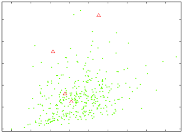
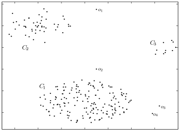
In real-world datasets, high dimensionality (e.g. 30 features) and sparse feature value range usually cause objects to be scattered in the feature space. The scattered data is similar to the distribution of stars in the universe. Locally, they seem to be randomly allocated in the night sky (i.e. stars observed from the Earth), whereas globally the stars constitute innumerable galaxies. Figure 1(a) illustrates a 2-D projection of a real-world dataset, Wisconsin Diagnostic Breast Cancer (WDBC)111WDBC dataset is from UCI ML Repository: http://archive.ics.uci.edu/ml., which is typically 30-D. The green points are the benign diagnosis records (regarded as normal objects), and the red triangles are malignant diagnosis records (i.e. outliers we want to capture). Obviously, we cannot detect these outliers in 2-D space, whereas in high dimension (e.g. 30-D), these scattered normal objects constitute a certain number of loosely bounded mini-clusters, and we are able to isolate genuine outliers. Unlike galaxies, which always contain billions of stars, these mini-clusters in scattered datasets usually have a relatively small number of objects. Figure 1(b) is a simple demonstration of this situation, where is a well-shaped cluster as we usually define in other outlier detection methods. and are comprised of scattered objects with loose boundary, called mini-clusters. These small clusters should be recognised as ‘normal’, even if they contain a small number of objects. The objects of our interest are the points lying far away from other mini-clusters. Intuitively, , , , are outliers in this sample. We recall a well accepted informal outlier definition proposed by Hawkins [Haw80]: “An outlier is an observation that deviates so much from other observations as to arouse suspicion that it was generated by a different mechanism”. In scattered datasets, an outlier should be an object deviating from any other group of objects.
The only way in which our outlier definition differs from others (e.g. in [KN98] and [BKNS00]) is that the normal pattern of data is represented by scattered objects, rather than crowded main clusters. The neighbourhood in scattered real-world datasets has two characteristics: (1) objects in mini-clusters are loosely distributed; (2) when neighbourhood size is large, two or more mini-clusters are taken into consideration. The neighbourhood becomes sparse as more and more objects which belong to different mini-clusters should be taken into account.
As discussed above, top- KNN and top- LOF are ineffective for scattered datasets. Take a typical example, in Figure 1(b), when is greater than the cardinality of (10 in this case), some objects in become neighbours of the objects in . Hence, for top- KNN, the -distance of the object can be larger than genuine outliers. For top- LOF, since the density of is smaller than that of , it also fails for ranking , , and in the highest outlier-ness positions. In Section 6, we will demonstrate that the two methods fail to detect genuine outliers when grows greater than 10.
Intuitively, it is more reasonable to measure how an object deviates from its neighbourhood system as an outlier-ness factor rather than global distance (top- KNN) or local density (top- LOF). Thereby, we propose LDOF to measure the degree of neighbourhood violation. The formal definition of LDOF is introduced in the following section.
3 Formal Definition of Local Distance-based Outliers
In this section, we develop a formal definition of the Local Distance-based Outlier Factor, which avoids the shortcomings presented above.
Definition 1 (KNN distance of )
Let be the set of the -nearest neighbours of object (excluding ). The -nearest neighbours distance of equals the average distance from to all objects in . More formally, let be a distance measure between objects and . The -nearest neighbours distance of object is defined as
Definition 2 (KNN inner distance of )
Given the -nearest neighbours set of object , the -nearest neighbours inner distance of is defined as the average distance among objects in :
Definition 3 (LDOF of )
The local distance-based outlier factor of is defined as:
If we regard the -nearest neighbours as a neighbourhood system, captures the degree to which object deviates from its neighbourhood system. It has the clear intuitive meaning that is the distance ratio indicating how far the object lies outside its neighbourhood system. When , it means that is surrounded by a data ‘cloud’. On the contrary, when , is outside the whole ‘cloud’. It is easy to see that the higher is, the farther is away from its neighbourhood system.
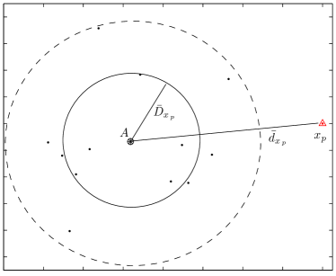
To further explain our definition, we exemplify it in Euclidian space. Hereinafter, let , and . For the squared Euclidian distance , the outlier definition can be written as:
| (1) | |||||
| (2) |
Thus, , i.e. lies outside its neighbourhood system, iff
| (3) |
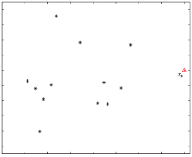
The same expression holds for the more general Mahalanobis distance [MKB79]. In Equation 3, the lefthand-side is the square distance of to its neighbourhood centroid , and the righthand-side becomes the distance variance in when . Therefore, Equation 6 can be understood as follows: The -nearest neighbours of object form a “reformed” neighbourhood region, represented as a hyperball with radius , centered at . As illustrated in Figure 2(a), since the neighbours of are scattered, it is unclear whether (indicated by ) belongs to its neighbourhood system or not. Our definition, as shown in Figure 2(b), it clearly regards as lying outside its reformed neighbourhood region. The of is obviously greater than 1, which indicates that is an outlier. Through this example we can see that can effectively capture the outlier-ness of an object among a scattered neighbourhood. In addition, as grows, takes more objects into consideration, and the view of becomes increasingly global. If an object is far from its large neighbourhood system (extremely the whole dataset) it is definitely a genuine outlier. Hence, the detection precision of our method might be stable over a large range of . In the following section, we will theoretically analyse properties of , and propose a heuristic for selecting the neighbourhood size .
4 Properties of LDOF
Lower bound of . Ideally, we prefer a universal threshold of to unambiguously distinguish abnormal from normal objects (e.g. in any datasets, an object is outlier if ). However, the threshold is problem dependent due to the complex structure of real-world datasets. Under some continuity assumption, we can calculate an asymptotic lower bound on , denoted as . indicates that an object is an inlier (or normal) if its is smaller than .
Theorem 4 ( lower-bound of outliers)
Let data be sampled from a density that is continuous at . For we have with high probability. More formally, for such that the neighbourhood size we have
The theorem shows that when , the point is squarely lying in a uniform cloud of objects, i.e. it is not an outlier. The lower-bound of provides a potential pruning rule of algorithm complexity. In practice, objects can be directly ignored if their s are smaller than . Remarkably, does not depend on the dimension of . This is very convenient: data often lie on lower-dimensional manifolds. Since locally, a manifold is close to an Euclidian space (of lower dimension), the result still holds in this case. Therefore, we do not need to know the effective dimension of our data.
Proof sketch. Consider data sampled from a continuous density (e.g. Gaussian or other standard distributions). For fixed , as sample size goes to infinity, the size of the -nearest neighbours region tends to zero. Locally any continuous distribution is approximately uniform. In the following we assume a uniform density around . The achieved result then generalizes to arbitrary distributions continuous at by taking the limit .
Without loss of generality, let . Fix some sufficiently small radius and let be the ball of radius around . By assumption, data is locally uniformly distributed, which induces a uniform distribution in , i.e. all are uniformly distributed random variables in . Hence their expected value . This implies
In the first equality we simply expanded the square in the definition of , where is the scalar product. In the second equality we used for . The last equality is just the definition of for . Taking the ratio we get
Note that the only property of the sampling distribution we used was , i.e. the result holds for more general distributions (e.g. any symmetric distribution around ).
Using the central limit theorem or explicit calculation, one can show that for large and , the distributions of and concentrate around their means and , respectively, which implies that with high probability.
This also shows that for any sampling density continuous at
(since they are locally approximately uniform), holds, provided . We
skip the formal proof.
False-detection probability. As discussed in Section 1, in real-world datasets, it is hard to set parameters properly by trial-and-error. Instead of requiring prior knowledge from datasets (e.g. outlier labels), we theoretically determine the false-detection probability, given neighbourhood size .
Theorem 5 (False-detection probability of LDOF)
Let data be uniformly distributed in a neighbourhood of containing objects . For threshold , the probability of false detecting as an outlier is exponentially small in . More precisely,
The bound still holds for non-uniform densities continuous in , provided .
In particular, for in high-dimensional spaces () we get . So for the false-detection probability is very small. Note that because the bound is quite crude, we can expect good performance in practice for much smaller . On the other hand, choosing degenerates the bound (i.e. ), consistent with Theorem 4.
Proof sketch. We follow the notation used in the proof of Theorem 4. We consider a uniform data distribution first. For and dropping , we can write the distances as
For uniformly distributed in ball , one can compute the mean square length explicitly:
| (5) |
where is the dimensionality of . The first equality is just the definition of a uniform expectation over . The second equality exploits rotational symmetry and reduces the -dimensional integral to a one-dimensional radial integral. The last equality is elementary. The expected values of and , respectively, are
| (6) | |||||
| (7) |
where we have exploited for . By rearranging terms, we see that
Thus we need (bounds on) the probabilities that and deviate (significantly) from their expectation. For any (vector-valued) i.i.d. random variables and any function symmetric under permutation of its arguments, McDiarmid’s inequality can be written as follows:
For an elementary calculation using gives . For we get straightforwardly. Now consider the real quantity of interest: . Combining the ranges, we can bound . The expectation of is . Let . Then using McDiarmid’s inequality we get
The last inequality follows from
where we have inserted , , and , and used and from the theorem. This proves the theorem for uniform distribution.
An analogous argument as in the proof of Theorem 4 shows
that the result still holds for non-uniform distributions if
, since a continuous density is locally
approximately uniform.
5 LDOF Outlier Detection Algorithm and Its Complexity
Top- LDOF. Even with the theoretical analysis of the previous section, it is still hard to determine a threshold for to identify outliers in an arbitrary dataset. Therefore we employ top- style outlier detection, which ranks the objects with the highest s. The algorithm that obtains the top- outliers for all the objects in a given dataset is outlined in Algorithm 1.
How to choose . Based on Theorem 5, it is beneficial to use a large neighbourhood size . However, too large will lead to a global method with the same problems as top- KNN outlier. For the best use of our algorithm, the lower bound of potentially suitable is given as follows: If the effective dimension of the manifold on which lies is , then at least points are needed to ‘surround’ another object. That is to say a is needed. In Section 6, we will see that, when increases to the dimension of the dataset, the detection performance of our method rises, and remains stable for a wide range of values. Therefore, the parameter in LDOF is easier to choose than in other outlier detection approaches.
Input: A given dataset , natural numbers and .
-
1.
For each object in , retrieve ’s -nearest neighbours;
-
2.
Calculate the for each object .
The objects with are directly discarded; -
3.
Sort the objects according to their values;
-
4.
Output: the first objects with the highest values.
Algorithm complexity. In Step 1, querying the -nearest neighbours, takes the majority of the computational load. Naively, the runtime of this step is . If a tree-based spatial index such as -tree or -tree is used [BKNS00, BKNS99], the complexity is reduced to . Step 2 is straightforward and calculates values according to Definition 3. As the - query is materialised, this step is linear in . Step 3 sorts the objects according to their values, which can be done in . Since the objects with are flushed (i.e. they are definitely non-outliers), the number of objects needed to sort in this step is smaller than in practice. Finally, the overall computation complexity of Algorithm 1 is with appropriate index support.
6 Experiments
In this section, we compare the outlier detection performance of top- LDOF with two typical top- outlier detection methods, top- KNN and top- LOF. Experiments start with a synthetic 2-D dataset which contains outliers that are meaningful but are difficult for top- KNN and top- LOF. In Experiments 2 and 3, we identify outliers in two real-world datasets to illustrate the effectiveness of our method in real-world situations. For consistency, we only use the parameter to represent the neighbourhood size in the investigation of the three methods. In particular, in top- LOF, the parameter MinPts is set to neighbourhood size as chosen in the other two methods.
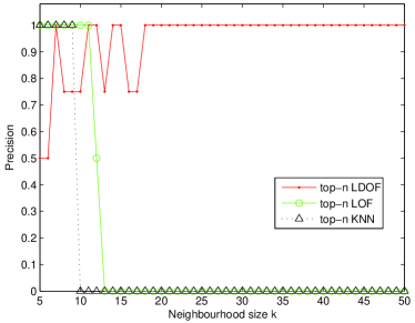
Synthetic Data. In Figure 1(b), there are 150 objects in cluster , 50 objects in cluster , 10 objects in cluster , and 4 additional objects which are genuine outliers. We ran the three outlier detection methods over a large range of . We use detection precision222Precision. We set as the number of real outliers if possible. to evaluate the performance of each method. In this experiment, we set (the number of real outliers). The experimental result is shown in Figure 3(a). The precision of top- KNN becomes 0 when the is larger than 10 due to the effect of the mini-cluster as we discussed in Section 2. For the same reason, the precision of top- LOF dramatically descends when is larger than 11. When the reaches 13, top- LOF misses all genuine outliers in the top-4 ranking (they even drop out of top-10). On the contrary, our method is not suffering from the effect of the mini-cluster. As shown in the Figure 3(a), the precision of our approach keeps stable at accuracy over a large neighbourhood size range (i.e. 20-50).
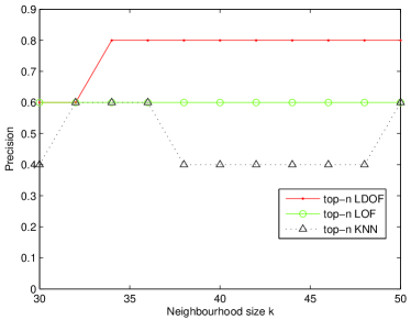
Medical Diagnosis Data. In real-world data repositories, it is hard to find a dataset for evaluating outlier detection algorithms, because only for very few real-world datasets it is exactly known which objects are really behaving differently [KSZ08]. In this experiment, we use a medical dataset, WDBC (Diagnosis)11footnotemark: 1, which has been used for nuclear feature extraction for breast tumor diagnosis. The dataset contains 569 medical diagnosis records (objects), each with 32 attributes (ID, diagnosis, 30 real-valued input features). The diagnosis is binary: ‘Benign’ and ‘Malignant’. We regard the objects labeled ‘Benign’ as normal data. In the experiment we use all 357 ‘Benign’ diagnosis records as normal objects and add a certain number of ‘Malignant’ diagnosis records into normal objects as outliers. Figure 3(b) shows the experimental result for adding the first 10 ‘Malignant’ records from the original dataset. Based on the rule for selecting neighbourhood size, , suggested in Section 4, we set in regards to the data dimension. We measure the percentage of real outliers detected in top-10 potential outliers as detection precision22footnotemark: 2. In the experiments, we progressively increase the value of and calculate the detection precision for each method. As shown in Figure 3(b), the precision of our method begins to ascend at , and keeps stable when is greater than 34 with detection accuracy of . In comparison, the precision of the other two techniques are towed over the whole value range.
To further validate our approach, we repeat the experiment 5 times with a different number of outliers (randomly extracted from ‘Malignant’ objects). Each time, we perform 30 independent runs, and calculate the average detection precision and standard deviation over the range from 30 to 50. The experimental results are listed in Table 1. The bold numbers indicate that the detection precision vector over the range of is statistically significantly improved compared to the other two methods (paired T-test at the 0.1 level).
| Number of outliers | Precision (mean std.) | ||
|---|---|---|---|
| LDOF | LOF | KNN | |
| 1 | 0.290.077 | 0.120.061 | 0.050.042 |
| 2 | 0.330.040 | 0.130.028 | 0.110.037 |
| 3 | 0.310.033 | 0.220.051 | 0.220.040 |
| 4 | 0.350.022 | 0.270.040 | 0.260.035 |
| 5 | 0.380.026 | 0.280.032 | 0.280.027 |
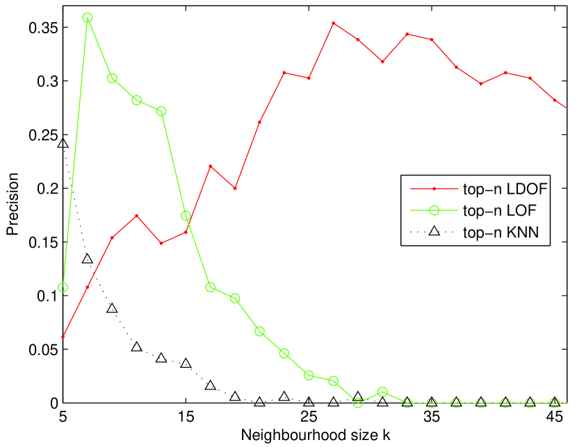
Space Shuttle Data. In this experiment, we use a dataset originally used for classification, named Shuttle333The Shuttle dataset can also be downloaded from UCI ML Repository.. We use the testing dataset which contains 14500 objects, and each object has 9 real-valued features and an integer label (1-7). We regard the (only 13) objects with label 2 as outliers, and regard the rest of the six classes as normal data. We run the experiment 15 times and each time we randomly pick a sample of normal objects (i.e. 1,000 objects) to mix with the 13 outliers. The mean values of detection precision of the three methods are presented in Figure 4. As illustrated in Figure 4, top- KNN has the worst performance (rapidly drops to 0). Top- LOF is better, which has a narrow precision peak ( from 5 to 15), and then declines dramatically. Top- LDOF has the best performance, as it ascends steadily and keeps a relative high precision over the range from 25 to 45. Table 4 shows the average precisions for the three methods over 15 runs. The bold numbers indicate that the precision vector is statistically significantly improved compared to the other two methods (paired T-test at the 0.1 level).
| Precision (mean std.) | ||
|---|---|---|
| LDOF | LOF | KNN |
| 0.250.081 | 0.030.057 | 0.080.114 |
7 Conclusion
In this paper, we have proposed a new outlier detection definition, LDOF. Our definition uses a local distance-based outlier factor to measure the degree to which an object deviates from its scattered neighbourhood. We have analysed the properties of LDOF, including its lower bound and false-detection probability. Furthermore, a method for selecting has been suggested. In order to ease the parameter setting in real-world applications, the top- technique has been used in this approach. Experimental results have demonstrated the ability of our new approach to better discover outliers with high precision, and to remain stable over a large range of neighbourhood sizes, compared to top- KNN and top- LOF. As future work, we are looking to extend the proposed approach to further enhance the outlier detection accuracy for scattered real-world datasets.
References
- [Bar94] V. Barnett. Outliers in Statistical Data. John Wiley, 1994.
- [BKNS99] Markus M. Breunig, Hans-Peter Kriegel, Raymond T. Ng, and Jörg Sander. OPTICS-OF: Identifying local outliers. In PKDD, pages 262–270, 1999.
- [BKNS00] Markus M. Breunig, Hans-Peter Kriegel, Raymond T. Ng, and Jörg Sander. LOF: Identifying density-based local outliers. In SIGMOD Conference, pages 93–104, 2000.
- [EKSX96] Martin Ester, Hans-Peter Kriegel, Jörg Sander, and Xiaowei Xu. A density-based algorithm for discovering clusters in large spatial databases with noise. In KDD, pages 226–231, 1996.
- [FZFW06] Hongqin Fan, Osmar R. Zaïane, Andrew Foss, and Junfeng Wu. A nonparametric outlier detection for effectively discovering top-n outliers from engineering data. In PAKDD, pages 557–566, 2006.
- [Haw80] D. Hawkins. Identification of Outliers. Chapman and Hall; London, 1980.
- [KN98] Edwin M. Knorr and Raymond T. Ng. Algorithms for mining distance-based outliers in large datasets. In VLDB, pages 392–403, 1998.
- [KSZ08] Hans-Peter Kriegel, Matthias Schubert, and Arthur Zimek. Angle-based outlier detection in high-dimensional data. In KDD, pages 444–452, 2008.
- [MKB79] K.V. Mardia, J.T. Kent, and J.M. Bibby. Multivariate analysis. Academic Press; New York, 1979.
- [RRS00] Sridhar Ramaswamy, Rajeev Rastogi, and Kyuseok Shim. Efficient algorithms for mining outliers from large data sets. In SIGMOD Conference, pages 427–438, 2000.
- [TCFC02] Jian Tang, Zhixiang Chen, Ada Wai-Chee Fu, and David Wai-Lok Cheung. Enhancing effectiveness of outlier detections for low density patterns. In PAKDD, pages 535–548, 2002.
- [Tuk77] J.W. Tukey. Exploratory Data Analysis. Addison-Wiley, 1977.