Spectral statistics of a pseudo-integrable map: the general case

Abstract

It is well established numerically that spectral statistics of pseudo-integrable models differs considerably from the reference statistics of integrable and chaotic systems. In [PRL 93 (2004) 254102] statistical properties of a certain quantized pseudo-integrable map had been calculated analytically but only for a special sequence of matrix dimensions. The purpose of this paper is to obtain the spectral statistics of the same quantum map for all matrix dimensions.

1 Introduction

The relation between spectral statistics of a quantum system and its classical counterpart is one of the main achievements of quantum chaos. It is established that at the scale of the mean level density the spectral statistics of classically integrable systems are described by the Poisson distribution [1] and the spectral statistics of classically chaotic systems are close to the statistics of eigenvalues of standard random matrix ensembles depending only on the underlying symmetry [2]. Though these statements had not mathematically been proved in the full generality and there exist noticeable exceptions (e.g. chaotic systems on constant negative curvature surfaces generated by arithmetic groups [3]), these conjectures are widely accepted for ’generic’ quantum systems.

Much less is known when a system is not classically integrable or completely chaotic. An important example which we have in mind is the case of pseudo-integrable systems (see e.g. [4]) represented by 2-dimensional polygonal billiards whose each angle is a rational multiple of $\pi$. A typical classical trajectory in such models covers a 2-dimensional surface of a finite genus $\geq 2$ [5]. For comparison, a trajectory of a 2-dimensional integrable model belongs to a 2-dimensional torus of genus 1 and a typical trajectory of a 2-dimensional chaotic system covers ergodically the whole 3-dimensional surface of constant energy.

Numerical calculations [6] clearly demonstrated that the spectral statistics of pseudo-integrable billiards is not universal and depends on billiard angles. It appears that spectral statistics of such models has two characteristic features: a level repulsion at small distances and an exponential decrease of the nearest-neighbour distribution at large separations. This type of statistics (called intermediate statistics) has been observed for the first time in the numerical simulations of the Anderson model at the point of metal-insulator transition [7] and later in this context has been profoundly investigated (see e.g. a recent review [8] and references therein). Unfortunately analytical progress in the investigation of intermediate statistics in pseudo-integrable systems is limited. In [9] the level compressibility of certain pseudo-integrable billiards was computed analytically, thus confirming the intermediate character of their spectral statistics. The main difficulty in analytical treatment of 2-dimensional pseudo-integrable billiards is the strong diffraction on billiard corners with angles $\neq\pi/n$ with integer $n$. Though there exists the exact Sommerfeld’s solution for the scattering on such angles [10], the diffraction coefficient is formally infinite along the optical boundaries so it is impossible to treat the multiple corner diffraction in perturbation series. A certain progress has been made in [11] where it was found that the multiple diffraction along periodic orbit channels in pseudo-integrable systems forces the wave functions to tend to zero on the channel boundaries thus forming superscarring states observed recently in micro-wave experiments [12].

The difficulties in analytical solution of pseudo-integrable billiards lead to the necessity of investigation of simpler models with similar features. A promising example is the quantization of interval exchange maps which are known to be the correct description of classical dynamics in pseudo-integrable systems [4], [5].

In [13] the following classical parabolic map had been quantized

$$\Phi_{\alpha}:\left(\begin{array}[]{c}p\\ q\end{array}\right)\Longrightarrow\left(\begin{array}[]{c}p+\alpha\\ q+f(p+\alpha)\end{array}\right)\;\mbox{ mod }1\ .$$ (1)

Here $\alpha$ is a constant and $f(p)$ is a certain function (taken equal $2p$ in [13]). For rational $\alpha=m/q$ this map corresponds to the simplest interval exchange map of 2 intervals.

After a straightforward generalization of the results of [13] the $N\times N$ unitary matrix associated with the above map has the form of the diagonal matrix $\mathrm{e}^{{\rm i}\Phi_{k}}$ with real $\Phi_{k}$ multiplied by a constant unitary matrix $\mu_{kp}$ ($k,p=0,1,\ldots,N-1$)

$$M_{kp}={\rm e}^{{\rm i}\Phi_{k}}\mu_{kp}\;,$$ (2)

where

$$\mu_{kp}=\frac{1}{N}\sum_{r=0}^{N-1}\exp\left[\frac{2\pi{\rm i}}{N}r(k-p+\alpha N)\right]=\frac{1-{\rm e}^{2\pi{\rm i}\alpha N}}{N(1-{\rm e}^{2\pi{\rm i}(k-p+\alpha N)/N})}\;.$$ (3)

The matrix $\mu_{kp}$ depends on a parameter $\alpha$ and the last equality are valid when $\alpha N$ is not an integer. (In the latter case the spectrum of (2) can be obtained analytically [14] and we always assume below that for rational $\alpha=m/q$, $mN\not\equiv 0$ mod $q$.)

Two main cases are of interest. The first corresponds to the ensemble of random matrices (2) where all $N$ phases $\Phi_{k}$ are considered as independent random variables distributed uniformly between $0$ and $2\pi$. We call such matrices non-symmetric ensemble.

In the second case only a half of the phases are independent random variables uniformly distributed between $0$ and $2\pi$. The other half is related to the first one by the symmetry

$$\Phi_{N-k}=\Phi_{k}\;,\;\;\;k=1,\ldots,\left[\frac{N}{2}\right].$$ (4)

This case will be called symmetric ensemble as in the dynamical interpretation the transformation $k\to-k$ is the time-inversion symmetry.

The eigenvalues $\Lambda_{n}$ and the eigenvectors $u_{k}(n)$, $n=1,2,\ldots,N$, are defined as usual

$$\Lambda_{n}u_{k}(n)=\sum_{p=0}^{N-1}M_{kp}u_{p}(n)\;.$$ (5)

Because matrix $M_{kp}$ is unitary ($M\,M^{{\dagger}}=1$), its eigenvalues lie on the unit circle

$$\Lambda_{n}={\rm e}^{{\rm i}\theta_{n}}$$ (6)

and its eigenvectors can be chosen orthogonal

$$\sum_{k=0}^{N-1}\bar{u}_{k}(m)u_{k}(n)=\delta_{mn}$$ (7)

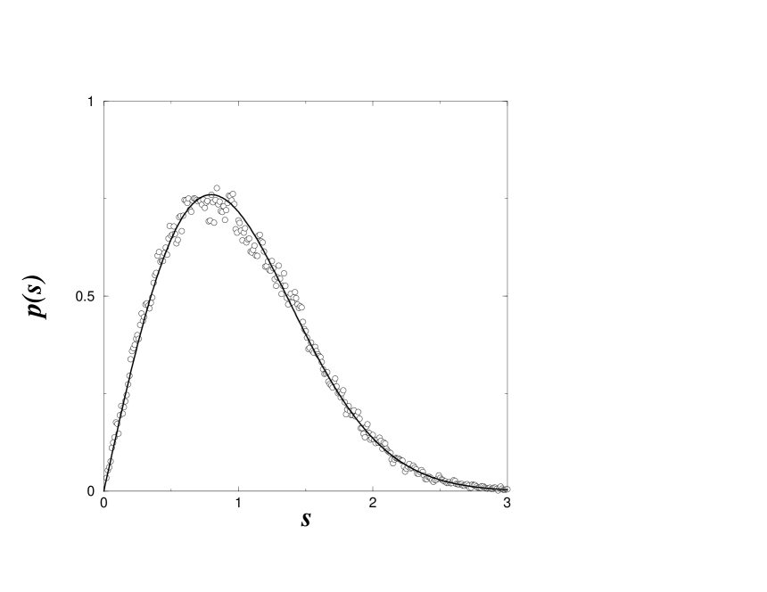
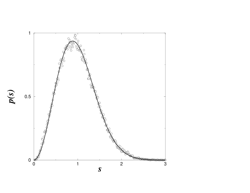
The statistical properties of matrix (2) depend crucially on the arithmetic of the parameter $\alpha$. For irrational $\alpha$ the map (1) is only a parabolic map and methods developed in [15] and in the present paper can not be directly applied. Numerical calculations suggest that for Diophantine $\alpha$ the spectral statistics of the matrix (2) is very close to the standard statistics of the Gaussian ensembles of random matrices [16]. Namely, non-symmetric matrices are described by the GUE statistics and symmetric matrices by the GOE statistics. For illustration in Fig. 1 we plot the nearest-neighbour distribution for matrices (2) with $\alpha=\sqrt{5}/4$ and $N=801$. The solid lines indicates the Wigner surmise (8) which is known (see e.g. [16]) to be a good approximation for the GUE and the GOE distributions.

a)

b)

Figure 1: Open circles are nearest-neighbour distribution with $\alpha=\sqrt{5}/4$ and $N=801$ for non-symmetric matrices (a) and symmetric matrices (b). Solid lines indicate the Wigner surmise (8).

$$p_{\mathrm{GUE}}(s)=\frac{32}{\pi^{2}}s^{2}\mathrm{e}^{-4s^{2}/\pi}\;,\;\;p_{\mathrm{GOE}}(s)=\frac{\pi}{2}s\mathrm{e}^{-\pi s^{2}/4}\ .$$ (8)

Rational $\alpha=m/q$ with co-prime integers $m$ and $q$ correspond to an interval exchange map [13] and we shall consider only such values of $\alpha$ throughout the paper.

This paper investigates the following question: What are the statistical properties of eigenvalues of the matrix (2) for fixed rational $\alpha=m/q$ and large $N$? It appears that to get a well defined limit in this case it is necessary to consider increasing sequences of matrix dimensions, $N$, such that the product of the numerator of $\alpha$ times $N$ has a fixed residue modulo the denominator of $\alpha$

$$mN\equiv k\;\;\mathrm{mod}\;\;q\ .$$ (9)

In [15] it was demonstrated that for a special sequence of matrix dimensions with

$$mN\equiv\pm 1\;\;\mathrm{mod}\;\;q$$ (10)

eigenvalues of the matrix (2), (3) are described by the so-called semi-Poisson statistics which has been proposed in [17] as the simplest model of intermediate statistics.

Let $x_{1}\leq x_{2}\leq\ldots\leq x_{K}$ be an ordered sequence of real numbers (eigenvalues). The joint distribution for the semi-Poisson statistics is proportional to the product of the nearest distances between these level times a confining potential $V(x)$

$$P(x_{1},x_{2},\ldots,x_{K})\sim\prod_{i}|x_{i+1}-x_{i}|^{\beta}\prod_{i}\mathrm{e}^{-V(x_{i})}$$ (11)

In the limit $K\to\infty$ all correlation functions of the semi-Poisson statistics at the scale of the mean level density do not depend on $V(x)$ and can be obtained analytically [17]. In particular, the probability that between 2 levels there exist exactly $n-1$ levels has the form

$$p_{n}(\beta;s)=\frac{(\beta+1)^{n\beta+n}}{\Gamma(n\beta+n)}s^{n\beta+n-1}\mathrm{e}^{-(\beta+1)s}\ .$$ (12)

The semi-Poisson statistics depends only on one parameter $\beta$ which fixes the level repulsion at small distances so the nearest-neighbour distribution (i.e. $p_{n}(\beta;s)$ for $n=1$) tends to zero as $s^{\beta}$

$$p(\beta;s)=A_{\beta}s^{\beta}\mathrm{e}^{-(\beta+1)s}$$ (13)

with $A_{\beta}=(\beta+1)^{\beta+1}/\Gamma(\beta+1)$.

From a mathematical point of view the semi-Poisson statistics can be considered as a stochastic process with independent increments (with gamma-distribution) forming a convolution semigroup

$$(p_{n}*p_{m})(\beta;s)\equiv\int_{0}^{s}p_{n}(\beta;y)p_{m}(\beta;s-y)\mathrm{d}y=p_{n+m}(\beta;s)\ .$$ (14)

According to [15] when the condition (10) is satisfied the spectral statistics of the matrix (2) tends for large $N$ to the semi-Poisson distribution with the following integer and half integer values of $\beta$ depending on the denominator of $\alpha=m/q$ and the symmetry of the map

$$\beta=\left\{\begin{array}[]{cl}q-1&\mbox{ for non-symmetric ensemble}\\ \frac{1}{2}q-1&\mbox{ for symmetric ensemble}\end{array}\right..$$ (15)

To compare numerical calculations with theoretical predictions it is often more precise to consider instead of the nearest-neighbour distribution, $p(s)$, (as in Fig. 1) its integral

$$N(s)\equiv\int_{0}^{s}p(s^{\prime})\mathrm{d}s^{\prime}$$ (16)

which gives the relative number of levels when the distance between the nearest-neighbour eigenvalues is less than $s$. This quantity is one of the main spectral correlation functions and throughout the paper we focus exclusively on it though other correlation functions can also be calculated and are of interest.

To illustrate the convergence of the spectral statistics of the above matrices to the predicted values let us consider e.g. $\alpha=1/2$ with odd $N$. From (15) and (13) it follows that the limiting integrated nearest-neighbour distribution in the non-symmetric case is here the simplest semi-Poisson distribution with $\beta=1$

$$N_{\mathrm{sp}}=1-(2s+1)\mathrm{e}^{-2s}\ .$$ (17)

In Fig. 2 the difference between the integrated nearest-neighbour distribution computed numerically and its theoretical prediction (17) is plotted for different odd matrix dimensions. For this and other similar figures in the paper the number of realizations is chosen to be the minimum between $100$ and $50000/N$. The figure shows that the agreement is quite good (less than $0.02$) even for $N$ of the order of a few hundreds.

Figure 2: Differences between the integrated nearest-neighbour distributions for the non-symmetric ensemble of matrices (2) with $\alpha=1/2$ for different odd $N$ and the theoretical prediction for this case (17). The different lines from bottom to top at small $s$ correspond, respectively, to $N=101$, $201$, $401$, $801$, and $1601$.

The purpose of this paper is to calculate the spectral statistics of the above quantized pseudo-integrable map in the general case (9) with $k\neq 0,\pm 1$ mod $q$. The plan of the paper is the following. Sections 2 and 3 give extended details of the construction briefly discussed in [15]. The peculiarity of the problem under consideration is the existence of 2 rank-one deformations of the original matrix (2) with known eigenvalues and eigenvectors. These deformations are discussed in Section 2. In Section 3 it is demonstrated that these rank-one deformations lead to long-range correlations between the eigenvalues of the initial matrix (2). To obtain a clear picture of these correlations it is convenient to use a special form of eigenvalue ordering (an analog of the unfolding) which is discussed in Section 4. In Section 5 it is shown that these long-range correlations can effectively be taken into account by the construction of a kind of transfer operator. This operator is a finite dimensional matrix whose largest eigenvalue and corresponding eigenvectors permit to calculate all correlation functions. This is done explicitly for a few main examples in Section 6. Obtained analytical formulas agree well with numerical calculations. The summary of the results is present in Section 7. Certain technical details are given in A.

2 Rank-one deformations

As was shown in [15] the important property of the matrix (2), (3) is the possibility to rewrite it in the following form

$$M_{kp}\equiv\mathrm{e}^{{\mathrm{i}}\Phi_{k}}\frac{(1-{\rm e}^{2\pi{\rm i}\alpha N})}{N(1-{\rm e}^{2\pi{\rm i}(k-p+\alpha N)/N})}=N_{kp}+\frac{1-{\rm e}^{2\pi{\rm i}\alpha N}}{N}{\rm e}^{{\rm i}\Phi_{k}}$$ (18)

where a new matrix $N_{kp}$ is

$$N_{kp}=M_{kp}{\rm e}^{2\pi{\rm i}(k-p+\alpha N)/N}\ .$$ (19)

Eigenvalues $\Lambda_{n}^{\prime}$ and eigenvectors $\psi_{k}(n)$ of the matrix $N_{kp}$

$$\Lambda_{n}^{\prime}\psi_{k}(n)=\sum_{p=0}^{N-1}N_{kp}\psi_{p}(n)$$ (20)

can easily be expressed through the eigenvalues and the eigenvectors of the original matrix $M_{kp}$

$$\psi_{k}(n)={\rm e}^{2\pi{\rm i}k/N}u_{k}(n)\;,\;\;\;\Lambda_{n}^{\prime}={\rm e}^{2\pi{\rm i}\alpha}\Lambda_{n}\;.$$ (21)

But from (18) it follows that matrix $N_{kp}$ is a rank-one deformation of matrix $M_{kp}$ so it is possible to construct its eigenvalues and corresponding eigenvectors in a different way (see e.g. [18]).

Write a formal expansion of an eigenvector of matrix $N_{kp}$ as a series of the complete set of eigenvectors of the matrix $M_{kp}$

$$\psi_{k}(n)\equiv{\rm e}^{2\pi{\rm i}k/N}u_{k}(n)=\sum_{m=1}^{N}c_{m}(n)u_{k}(m)\ .$$ (22)

From (18) one gets

$$\Lambda_{n}^{\prime}\sum_{m=1}^{N}c_{m}(n)u_{k}(m)=\sum_{m=1}^{N}c_{m}(n)\Lambda_{m}u_{k}(m)-\frac{1-{\rm e}^{2\pi{\rm i}\alpha N}}{N}{\rm e}^{{\rm i}\Phi_{k}}\sum_{m=1}^{N}c_{m}(n)\sum_{p=0}^{N-1}u_{p}(m)\ .$$ (23)

Introducing the notations

$$A_{m}=\sum_{k=0}^{N-1}u_{k}(m)\ ,\;\;\;g(n)=\sum_{m=1}^{N}c_{m}(n)A_{m}$$ (24)

and using the orthogonality of eigenvectors $u_{k}(n)$ (7) one obtains

$$c_{m}(n)=\frac{1-{\rm e}^{2\pi{\rm i}\alpha N}}{N}g(n)\frac{B_{m}}{\Lambda_{m}-\Lambda^{\prime}_{n}}\;$$ (25)

where

$$B_{m}=\sum_{k=0}^{N-1}{\rm e}^{{\rm i}\Phi_{k}}\bar{u}_{k}(m)\;.$$ (26)

Multiplying the both sides of (25) by $A_{m}$ and summing from 1 to $N$ one concludes that every eigenvalues $\Lambda^{\prime}_{m}$ of the matrix $N_{kp}$ obey the equation

$$1=\frac{1-{\rm e}^{2\pi{\rm i}\alpha N}}{N}\sum_{m=1}^{N}\frac{A_{m}B_{m}}{\Lambda_{m}-\Lambda^{\prime}_{n}}\ .$$ (27)

From (5) and (3) it follows that

$$\Lambda_{m}B_{m}^{*}=A_{m}$$ (28)

and Eq. (27) takes the final form

$$1=\frac{1-{\rm e}^{2\pi{\rm i}\alpha N}}{N}\sum_{m}\frac{\Lambda_{m}|B_{m}|^{2}}{\Lambda_{m}-\Lambda^{\prime}_{n}}\ .$$ (29)

For rank-one deformations of a real symmetric matrix all terms in the corresponding equation would be real and one easily comes to the well known conclusion that eigenvalues of a rank-one deformation of a real symmetric matrix are in-between eigenvalues of the unperturbed ones (cf. [18]). In our case the both matrices, $M_{kp}$ and $N_{kp}$ are unitary and their eigenvalues lie on the unit circle: $\Lambda_{m}={\rm e}^{{\rm i}\theta_{m}}$, $\Lambda^{\prime}_{n}={\rm e}^{{\rm i}\theta^{\prime}_{n}}$. So arguments require straightforward modifications.

From (29) one gets

$$\frac{N}{1-{\rm e}^{2\pi{\rm i}\alpha N}}=\sum_{m}\frac{|B_{m}|^{2}}{1-{\rm e}^{{\rm i}(\theta^{\prime}_{n}-\theta_{m})}}$$ (30)

which can be rewritten as follows

$$N(\cot\pi\alpha N-{\rm i})=\sum_{m}|B_{m}|^{2}\left(\cot\frac{\theta^{\prime}_{n}-\theta_{m}}{2}-{\rm i}\right)\ .$$ (31)

Due to the completeness of $u_{k}(m)$ one has

$$\sum_{n=1}^{N}\bar{u}_{p}(n)u_{k}(n)=\delta_{pk}\;.$$ (32)

and, consequently,

$$\sum_{m=1}^{N}|B_{m}|^{2}=N\ .$$ (33)

Therefore, the imaginary part of (31) is identically zero and new phases $\theta^{\prime}_{n}$ have to be determined from a real equation

$$F(\theta^{\prime}_{n})=N\cot\pi\alpha N$$ (34)

where $F(\theta)$ is defined by:

$$F(\theta)=\sum_{m=1}^{N}|B_{m}|^{2}\cot\frac{\theta-\theta_{m}}{2}\;.$$ (35)

In the interval $[0,2\pi)$ $F(\theta)$ has poles at $\theta=\theta_{m}$ (assuming that all $B_{m}\neq 0$) and it is monotone between them (cf. Fig. 3). Let the eigenphases $\theta_{m}$ be ordered on the unit circle $0\leq\theta_{1}\leq\theta_{2}\leq\ldots\leq\theta_{N}<2\pi$. Then between two near-by eigenvalues $\theta_{m}$ and $\theta_{m+1}$ (mod $2\pi$) there exists one and only one new eigenvalue $\theta^{\prime}_{n}$. Here the new eigenvalues are not necessarily ordered.

Figure 3: Schematic plot of Eq. (34) (solid black line). $F(\theta)$ is defined by (35). Vertical dashed lines represent the pole positions. Horizontal straight line indicates the value of the right-hand sine of Eq. (34). The abscissa of its intersections with $F(\theta)$ (indicated by black circles) give the solutions of that equation.

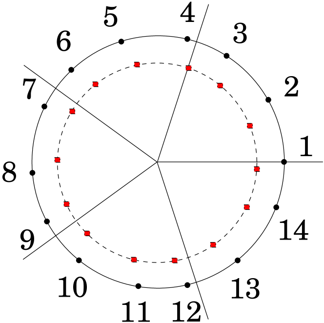
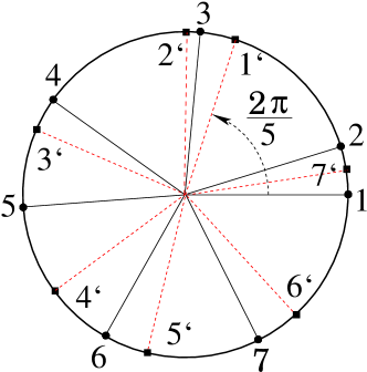
But according to (21) all eigenphases of the matrix $N_{kp}$ have the form $\theta^{\prime}_{m}=\theta_{m}+2\pi\alpha$ (mod $2\pi$). Therefore we prove the following lemma (cf. Fig. 4).Lemma 1. The eigenvalues of the unitary matrix $M_{kp}$ defined in (2) and (3) are such that after the rotation by $2\pi\alpha$ in-between of any pairs of nearest eigenvalues there exist one and only one rotated eigenvalue.

Figure 4: Illustration of Lemma 1. Black circles denote the position of 7 eigenphases for $\alpha=1/5$ and black lines are their radius-vectors. Black squares indicate the position of eigenphases after the rotation by angle $2\pi/5$ and dashed red lines are radius-vectors of the rotated eigenphases. The rotated points are indicated by the same number but with sign ^′.

Multiplying (18) by $\exp(-2\pi{\rm i}(k-p+\alpha N)/N)$ one gets another relation

$$M_{kp}=\tilde{N}_{kp}-\frac{1-{\rm e}^{2\pi{\rm i}\alpha N}}{N}{\rm e}^{{\rm i}\Phi_{k}-2\pi{\rm i}(k-p+\alpha N)/N}$$ (36)

with a new matrix $\tilde{N}_{kp}$

$$\tilde{N}_{kp}=M_{kp}{\rm e}^{-2\pi{\rm i}(k-p+\alpha N)/N}$$ (37)

whose eigenvalues and eigenvectors are

$$\tilde{\psi}_{k}(n)={\rm e}^{-2\pi{\rm i}k/N}u_{k}(n)\;,\;\;\;\tilde{\Lambda}_{n}^{\prime}={\rm e}^{-2\pi{\rm i}\alpha}\Lambda_{n}\;.$$ (38)

Repeating the above calculations but for the matrix $\tilde{N}_{kp}$ one finds that its eigenvalues $\tilde{\Lambda}^{\prime}_{m}$ have to be determined from the equation

$$1=\frac{1-{\rm e}^{2\pi{\rm i}\alpha N}}{N}\sum_{m=1}^{N}\frac{\Lambda_{m}|\tilde{B}_{m}|^{2}}{\Lambda_{m}-\tilde{\Lambda}^{\prime}_{n}}$$ (39)

where

$$\tilde{B}_{m}=\sum_{k=0}^{N-1}\bar{u}_{k}(m){\rm e}^{{\rm i}\Phi_{k}-2\pi{\rm i}k/N}$$ (40)

As it has exactly the same form as (29) and $\tilde{\Lambda}_{n}^{\prime}={\rm e}^{-2\pi{\rm i}\alpha}\Lambda_{n}$ one comes to the lemma.Lemma $1^{\prime}$. The eigenvalues of $M_{kp}$ are such that after the rotation by $-2\pi\alpha$ between two nearest eigenvalues of $M_{kp}$ there exists one and only one rotated eigenvalue. These lemmas prove the existence of long-range correlations between eigenvalues of the matrix $M_{kp}$ which are merely a consequence of the fact that rank-one deformations (18) and (36) of the original matrix (2) have eigenvalues easily expressible through eigenvalues of the original matrix.

A few other consequences of this property is worth to mention. As all $N$ solutions of (29) have the form $\Lambda^{\prime}_{n}=\Lambda_{n}{\rm e}^{2\pi{\rm i}\alpha}$ with $n=1,\ldots,N$ the numerators of this equation can be found explicitly. From A it follows that

$$\frac{1-{\rm e}^{2\pi{\rm i}\alpha N}}{N}\Lambda_{m}|B_{m}|^{2}=\frac{\displaystyle\prod_{n=1}^{N}(\Lambda_{m}-\Lambda_{n}{\rm e}^{2\pi{\rm i}\alpha})}{\displaystyle\prod_{s\neq m}(\Lambda_{m}-\Lambda_{s})}$$ (41)

which can be rewritten in the real form as follows

$$|B_{m}|^{2}\frac{\sin\pi\alpha N}{N\sin\pi\alpha}=\prod_{n\neq m}\frac{\sin(\frac{1}{2}(\theta_{m}-\theta_{n}-2\pi\alpha))}{\sin(\frac{1}{2}(\theta_{m}-\theta_{n}))}\ .$$ (42)

Similarly, from (39) one concludes that

$$\frac{1-{\rm e}^{-2\pi{\rm i}\alpha N}}{N}\Lambda_{m}|\tilde{B}_{m}|^{2}=\frac{\displaystyle\prod_{n=1}^{N}(\Lambda_{m}-\Lambda_{n}{\rm e}^{-2\pi{\rm i}\alpha})}{\displaystyle\prod_{s\neq m}(\Lambda_{m}-\Lambda_{s})}\ .$$ (43)

So

$$|\tilde{B}_{m}|^{2}\frac{\sin\pi\alpha N}{N\sin\pi\alpha}=\prod_{n\neq m}\frac{\sin(\frac{1}{2}(\theta_{m}-\theta_{n}+2\pi\alpha))}{\sin(\frac{1}{2}(\theta_{m}-\theta_{n}))}\ .$$ (44)

3 Long-range correlations

In the preceding Sections it has been proved that eigenphases of matrix (5) have a special type of long-range correlations. Namely, when one rotates all eigenvalues of this matrix by $\pm 2\pi\alpha$ and superimposes the rotated eigenphases with non-rotated ones then in-between two nearest eigenvalues of the original matrix there will be one and only one rotated eigenphase. In this Section we investigate certain consequences of such correlations in more details.

Let us put all eigenvalues of unitary matrix (2) on the unit circle and consider a sector of angle $2\pi\alpha$ which contains $n$ eigenvalues (see Fig. 5a).

a)

b)

Figure 5: (a) Eigenphases close to the boundaries of a $2\pi\alpha$ sector. (b) Division of the unit circle into sectors of angle $2\pi m/q$. Black circles indicate the position of eigenphases in two near-by sectors. Dashed lines show the positions which will occupy eigenvalues from one sector after the rotation by $2\pi m/q$.

The sector boundaries divide the unit circle in-between certain eigenphases. Denote the angular distance from the sector boundaries to the nearest eigenphases in the clockwise and counterclockwise directions by $y_{k}$, $y_{k+1}$ and $x_{k}$, $x_{k+1}$ respectively (cf. Fig. 5a). After the rotation by $2\pi\alpha$ only 2 possibilities are possible: either the point $x_{k}$ or the point $y_{k}$ will fall inside the points $x_{k+1}$ and $y_{k+1}$. In the first case one has $x_{k}<x_{k+1}$ and $y_{k+1}<y_{k}$. In the second case the inequalities are reversed: $x_{k}>x_{k+1}$ and $y_{k+1}>y_{k}$. Therefore in the all cases the following inequality is fulfilled

$$(y_{k+1}-y_{k})(x_{k+1}-x_{k})<0\ .$$ (45)

This inequality is valid for all $\alpha$ and $N$. From now on we shall consider only rational $\alpha$

$$\alpha=\frac{m}{q}$$ (46)

with co-prime integers $m$ and $q$.

As above divide the unit circle into $q$ radial sectors of angle $2\pi m/q$. When $m=1$ these sectors are disjoint but for $m>1$ they will overlap. Denote the number of eigenphases in the $k^{\mbox{th}}$ sector by $n_{k}$ (see Fig. 5b).

After the rotation by $2\pi m/q$ the eigenphases from the $k^{\mbox{th}}$ sector will move into the $(k+1)^{\mbox{th}}$ sector. These rotated points will divide this sector into $n_{k}+1$ intervals. According to the lemma $1$ the eigenphases in the $(k+1)^{\mbox{th}}$ sector have to be intertwined with the rotated eigenvalues. Therefore, all intervals except the first and the last have to be occupied. The first will be occupied if $x_{k}>x_{k+1}$ and the last will be occupied if $y_{k+1}>y_{k+2}$. All these requirements can be rewritten as the following recurrence relation

$$n_{k+1}=n_{k}-1+\Theta(x_{k}-x_{k+1})+\Theta(y_{k+1}-y_{k+2})\ .$$ (47)

Here as in Fig. 5a $x_{k}$ and $y_{k}$ are distances from the boundary of the $k^{\mbox{th}}$ sector to the two closest eigenphases to it and $\Theta(x)$ is the Heaviside function: $\Theta(x)=1$ if $x>0$ and $\Theta(x)=0$ if $x<0$. From (45) it follows that the difference $y_{k+1}-y_{k+2}$ is of the opposite sign than the the difference $x_{k+1}-x_{k+2}$ and the last relation takes the form

$$n_{k+1}=n_{k}-1+\Theta(x_{k}-x_{k+1})+\Theta(x_{k+2}-x_{k+1})\ .$$ (48)

Now choose the beginning of the first sector at the position of an eigenphase (i.e. impose $y_{1}=0$). Then from (45) it follows that $x_{2}<x_{1}$ and $x_{q}<x_{1}$. Direct applications of (48) give

$$n_{2}=n_{1}-1+\Theta(x_{1}-x_{2})+\Theta(x_{3}-x_{2})=n_{1}+\Theta(x_{3}-x_{2})$$ (49)

because $x_{1}>x_{2}$,

$$n_{3} = n_{2}-1+\Theta(x_{2}-x_{3})+\Theta(x_{4}-x_{3})$$ (50)

$$= n_{1}+\Theta(x_{3}-x_{2})-1+\Theta(x_{2}-x_{3})+\Theta(x_{4}-x_{3})=n_{1}+\Theta(x_{4}-x_{3})$$

because $\Theta(x)+\Theta(-x)=1$ and so on. In this manner one concludes that for $j=2,\ldots,q-1$

$$n_{j}=n_{1}+\Theta(x_{j+1}-x_{j})$$ (51)

and $n_{q}=n_{1}+1$ because, as was noted above, $x_{q}<x_{1}$.

As the sum over all $q$ sectors cover the unit circle $m$ times, the sum over all $n_{k}$ equals $mN$: $\displaystyle\sum_{k=1}^{q}n_{k}=mN$. Therefore

$$mN=qn_{1}+1+\sum_{j=2}^{q-1}\Theta(x_{j+1}-x_{j})\ .$$ (52)

When $mN\equiv 1$ mod $q$, all $\Theta$-functions in the right-hand side of this expression are forced to be zero which leads to the conclusion that in this case

$$x_{q}<x_{q-1}<\ldots<x_{2}<x_{1}\ .$$ (53)

When $mN\equiv-1$ mod $q$, all $\Theta$-functions have to be equal to 1 and the inequalities are reversed

$$x_{2}<x_{3}<\ldots<x_{q-1}<x_{q}<x_{1}\ .$$ (54)

Inequalities (53) and (54) manifest the existence of an exceptionally strong long-range correlations when $mN\equiv\pm 1$ mod $q$. For usual matrix ensembles correlations between eigenvalues separated by a large distance tend to zero. But in our case eigenphases at distances $2\pi mk/q$ with $k=1,\ldots,(q-1)$ are not independent but restricted by the above inequalities. In [15] only these special cases had been considered.

4 Geometrical unfolding

To visualize better the restrictions implied by inequalities (45) and recurrence relations (48) let us split the unit circle into $q$ angular sectors of angle $2\pi m/q$ as above and denote the positions of eigenvalues inside each sector on $q$ parallel lines (see Fig. 6).

a)

b)

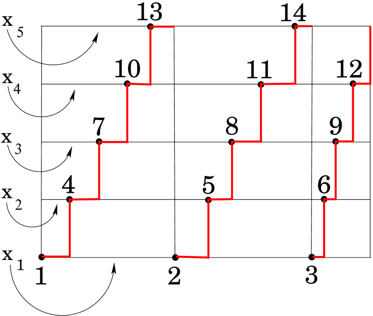
Figure 6: (a) Small black circles: schematic view of eigenvalues of matrix (2) for $\alpha=1/5$ and $N=14$ ($N\equiv-1$ mod $5$). Numbers from 1 to 14 indicate the consecutive eigenphases. Eigenphases rotated by $2\pi/5$ are denoted by red squares. For clarity they are situated on a smaller dashed circle. (b) The same configuration of eigenvalues but unfolded on 5 horizontal lines representing 5 sectors. $x_{1},\ldots,x_{5}$ are the distances from the beginning of the sectors to the closest eigenphase as in Fig. 5a. Thick red lines demonstrate relative eigenvalue positions.

According to Lemmas 1 and $1^{\prime}$, between two closest eigenphases of the matrix (2) there is one and only one eigenphase rotated by $2\pi\alpha=2\pi m/q$. In the unfolded description it is manifested by the condition that points at each line have to be in-between two close-by points on the lower line. The relative positions of eigenvalues strongly depend on distances $x_{k}$ from the beginning of each sector to the eigenphase closest to it (see (52)). In the unfolded representation (as in Fig. 6a) $x_{k}$ are the distances along the horizontal lines to points closest to a vertical line which represents the boundary of a sector with angle $2\pi m/q$.

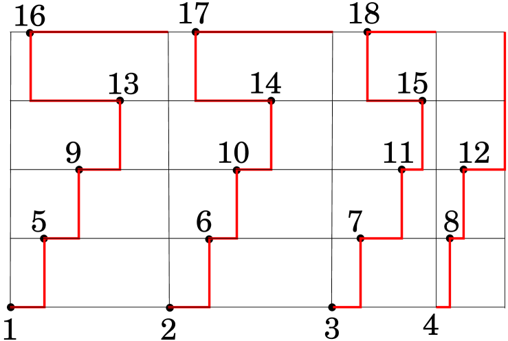
Let start from the lower left point and draw a horizontal line till there is at the vertical a point situated at the first line above it. Then draw the vertical line till it touches that point. Now continue drawing an horizontal line till there is at the vertical a point at the upper line closest to the boundary of the given sector and so on. This line will go right if $x_{k+1}>x_{k}$ and left if $x_{k+1}<x_{k}$. Finally, points will be connected by step-wise lines as in Fig. 6b. Notice that according to our convention point 1 does not belong to the first line but to the last one. The shape of these lines are determined by the inequalities between all $x_{k}$. In Fig. 6 the case of $N\equiv-1$ mod $5$ is indicated. According to (54) $x_{k+1}>x_{k}$ for $k=1,\ldots,4$ which explains the staircase form of these lines. They all start at points along the first horizontal line, go up and to the right, and finally finish at the last horizontal line but with the shift by 1 unit. It is clear that such lines cannot cross each other.

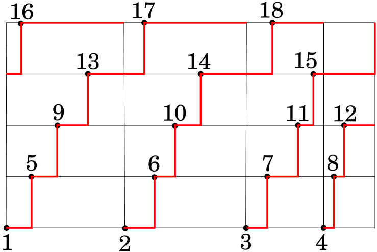
For other matrix dimensions these lines will have a different shape. Consider first as an example the case $\alpha=1/5$ and $N\equiv 3$ mod $5$. From (52) it follows that in this case only 2 of 3 $\Theta$-functions have to be equal to 1. Every time one of the $\Theta$-function is zero, the above lines turns to the left (see Fig. 7) so the shape of the step-wise curve differs from the one of Fig. 6b. Consider the horizontal line when it first turns left. Instead of the left turn let us continue to the right till we touch an other point on this line. As between these two points there exists only one point at the lower and higher lines there is no contradiction with our line construction (cf. Fig. 7). Finally we come to the conclusion that for these values of $\alpha$ and $N$ the eigenphases have to be connected by non-intersecting lines which go only up and to the right and whose initial and final points are shifted by 2 units.

a)

b)

Figure 7: (a) Small black circles: schematic view of eigenvalues of matrix (2) for $\alpha=1/5$ and $N=18$ (i.e. $N\equiv-2$ mod $5$). Thick red lines connect eigenphases as indicated in the text. (b) The same configuration of eigenvalues but connected by non-decreasing staircase lines.

These arguments can be generalized for all values of matrix dimensions and we get the following lemma.
Lemma 3: For $\alpha=m/q$ and $mN\equiv k$ mod $q$ with $k=1,\ldots,q-1$ mutual positions of eigenphases of matrix (2) can be described as follows. Fix $q$ horizontal lines, put arbitrary points at the lowest line, and notice the vertical images of these points along the last line. Draw staircase non-intersecting lines going only up and to the right with the condition that they start at the lower line and end at last line but with the shift by $k$ units. Points at horizontal lines are situated at the corners of the constructed lines.

When $k>q/2$ one may simplify the construction by using non-intersecting step-wise lines going up and to the left with the shift by $q-k$. It implies that properties of the cases $mN\equiv k$ mod $q$ and $mN\equiv-k$ mod $q$ are the same.

5 Transfer operator

The above unfolding gives not only a clear picture of mutual positions of eigenphases but also serves as the basis of the explicit calculation of the spectral statistics for the problem under consideration. The calculations are based on the following conjecture proposed in [15].

Conjecture: For $\alpha=m/q$ the eigenvalues of the $q^{\mathrm{th}}$ power of the original matrix (2) for all $N\not\equiv 0$ mod $q$ have universal spectral statistics independent on $q$ and $N$ but different for different symmetry classes of random phases $\Phi_{k}$. For non-symmetric ensemble the statistics of $M^{q}$ coincides with the Poisson statistics and for symmetric ensemble (4) it is described by the semi-Poisson statistics with $\beta=-1/2$ called in [15] the super-Poisson statistics.

The main physical argument in favor of this conjecture in [15] was the fact that for rational $\alpha=m/q$ the $q^{\mathrm{th}}$ power of the classical map (1) corresponds to a classically integrable map, and according to the usual wisdom [1] integrable models have to be described by the Poisson statistics. Extensive numerical calculations agree very well with this conjecture. But it seems that to prove it rigorously one has to develop new methods which are at present under investigation [19].

After unfolding, when the points from all the sectors separated by $2\pi m/q$ are taken together, they can be considered as the eigenphases of the $q^{\mathrm{th}}$ power of the original matrix (with evident rescaling). Assuming the validity of the conjecture it follows that for all $N\not\equiv 0$ mod $q$ these points constitute the semi-Poisson ensemble with $\beta=0$ for non-symmetric matrices and $\beta=-1/2$ for symmetric ones.

In particular, the probability that between two eigenvalues of $M^{q}$ separated by $x$ there exist exactly $r$ eigenvalues is the following

$$p_{r}(x)=\left\{\begin{array}[]{cl}\displaystyle\frac{x^{r}}{r!}\mathrm{e}^{-x}&\mathrm{for\;non-symmetric\;ensemble}\\ \displaystyle\frac{1}{2^{(r+1)/2}\Gamma((r+1)/2)}x^{(r-1)/2}\mathrm{e}^{-x/2}&\mathrm{for\;symmetric\;ensemble}\end{array}\right..$$ (55)

The results of the preceding Section can be reformulated such that the joint probability of the close-by levels integrated over all the possible positions of other levels is the same as the probability of non-intersecting staircase lines which start from the initial levels and which finish after $q$ steps (where $q$ is the denominator of $\alpha$) with the shift of $k$ units (where $k$ is the residue of $mN$ modulo $q$). According to the conjecture the distribution of unfolded points are known which permits the calculation of spectral statistics of the original matrix (2).

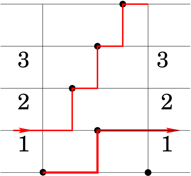
The usual method of computing the probability of non-intersecting paths in a Markoff process is the determinantal representation [20]. We found that for practical reasons it is more convenient to use the transfer operator method. In this method one first unfolds the spectrum as indicated in Fig. 7. Then one considers a vertical strip bounded by vertical lines emanating from any two near-by levels of original matrix, say $x_{2}$ and $x_{3}$ in Fig. 7 separated by the distance $x=x_{3}-x_{2}$. Now different horizontal lines can enter and can leave the strip. When all in-coming and out-coming horizontal lines are fixed, it is obvious that the configuration inside the strip is not affected by outside points. Therefore, it is possible to integrate over all configurations of points inside the strip with prescribed ordering. Denoting the initial and final lines by indexes $i$ and $j$ the result of integration constitutes the matrix element $T_{ji}(x)$ of the transfer matrix $T(x)$.

For rational $\alpha=m/q$ and $mN\equiv k$ mod $q$ with $1\leq k\leq q-1$ each initial (and final) state is determined by fixing $l=q-k-1$ horizontal lines

$$1\leq i_{1}<i_{2}<\ldots<i_{l}\leq q-2$$ (56)

from the total number of lines equal $q-2$. It means that the dimension of the transfer operator is

$$t=C_{q-2}^{l}$$ (57)

and it is convenient to label the set of $l$ integers obeying (56) in e.g. lexicographical order.

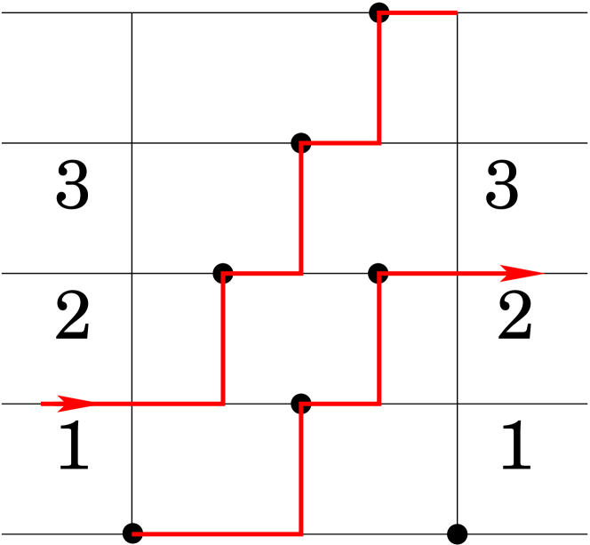
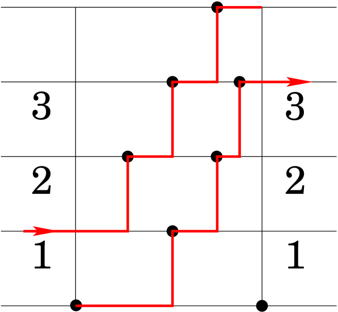
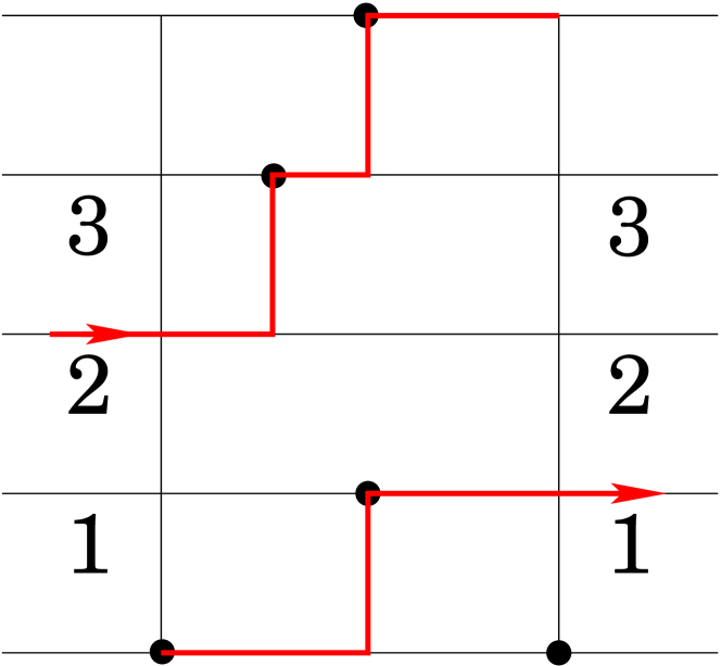
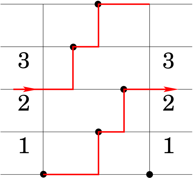
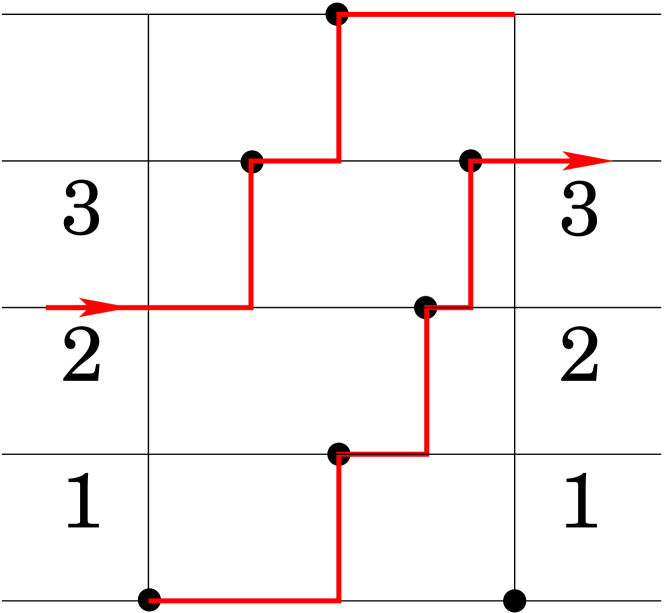
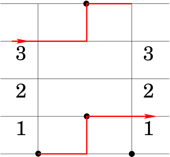
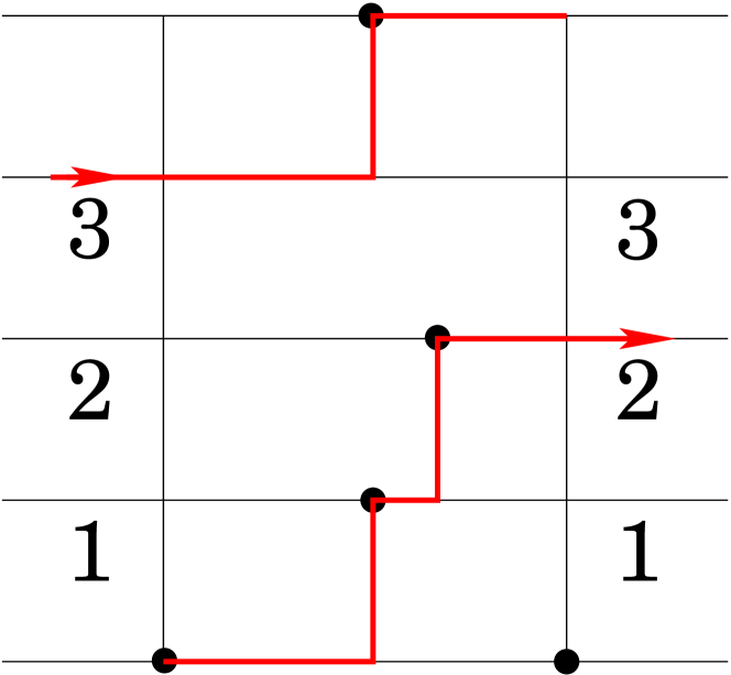
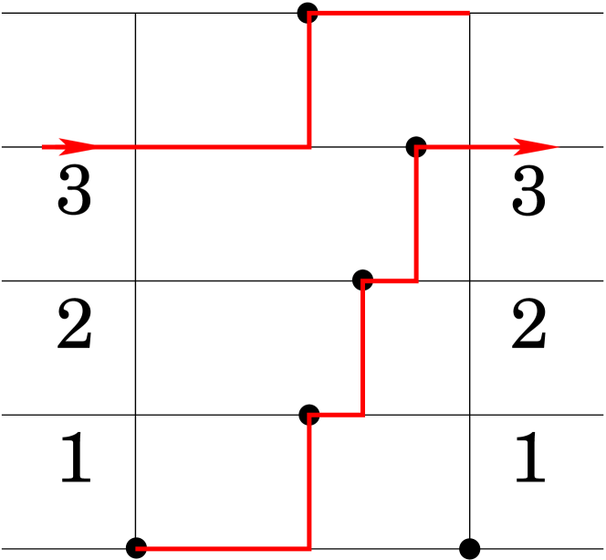
For clarity, let us consider the case $\alpha=1/5$ and $N\equiv 3$ mod $5$ in detail ($l=1$). As $q=5$ there is one possible horizontal line which may go through the vertical strip (cf. Fig. 7). Therefore the transfer matrix is $3\times 3$ matrix labeled by the number of these lines. In Fig. 8 all possible configurations for this case are presented.

$T_{11}$

$T_{12}$

$T_{13}$

$T_{21}$

$T_{22}$

$T_{23}$

$T_{31}$

$T_{32}$

$T_{33}$

Figure 8: Structure of the transfer operator for $\alpha=1/5$ and $N\equiv-2$ mod $5$.

In general, if $i\equiv(i_{1},i_{2},\ldots,i_{l})$ and $j\equiv(j_{1},j_{2},\ldots,j_{l})$ are multi-indexes of an initial and a final states, the total number of points, $r$, inside the considered vertical strip is determined by the expression

$$r=j_{1}+\sum_{s=1}^{l-1}[j_{s+1}-i_{s}]+q-1-i_{l}=|j|-|i|+q-1$$ (58)

where $|j|\equiv j_{1}+\ldots+j_{l}$ and $|i|\equiv i_{1}+\ldots+i_{l}$. In general, $r_{\mathrm{min}}\leq r\leq r_{\mathrm{max}}$ with

$$r_{\mathrm{min}}=2\ ,\;\;r_{\mathrm{max}}=k(q-k)\ .$$ (59)

If at least one term in the square brackets in (58) is negative, the configuration is impossible and the corresponding matrix element equals zero. Otherwise, the integration over all intermediate configurations compatible with the imposed inequalities gives the value of the transfer matrix elements.

The calculation of this probability is straightforward. According to the above conjecture, the probability that between 2 eigenvalues of $M^{q}$ separated by $x$ there exist $r$ ordered eigenvalues $y_{s}$ such that

$$0\leq y_{1}\leq y_{2}\leq\ldots\leq y_{r}\leq x$$ (60)

is given by (55). Therefore, the transfer matrix element $T_{ji}(x)$ is the product of 2 factors

$$T_{ji}(x)=n_{ji}p_{r}(x)$$ (61)

where $r$ is the integer determined by (58), $p_{r}(x)$ is the same as in (55), and $n_{ji}$ is the number of configurations of $r$ points which fulfilled all inequalities comparable with the fixed initial and final states. Interchanging the initial and final states and counting horizontal lines from the top one gets that the transfer operator matrix elements obey the following symmetry

$$T_{ji}(x)=T_{i^{T}j^{T}}(x)$$ (62)

where if $i=(i_{1},\ldots,i_{l})$, $i^{T}=(q-1-i_{l},\ldots,q-1-i_{1})$.

For example, for $\alpha=1/5$ and $N\equiv-2$ mod $5$ the $T_{12}$ element includes 5 points (cf. Fig. 8), 3 points, $a$, $b$, $c$ belong to the upper curve, and 2 points, $A$ and $B$, belong to the lower curve. From the mutual positions of these points it follows that the $T_{12}(x)$ matrix element equals the probability that the following inequalities are fulfilled

$$0\leq a\leq b\leq c\leq x,\;\;0\leq A\leq B\leq x,\;\;a\leq A,\;\;b\leq B.$$ (63)

By inspection one finds that there exist exactly 5 possible ordered sequences compatible with inequalities (63), namely

$$a\ b\ c\ A\ B,\;\;\;a\ b\ A\ B\ c,\;\;\;a\ A\ b\ B\ c,\;\;\;a\ b\ A\ c\ B,\;\;\;a\ A\ b\ c\ B.\;\;\;$$

Therefore $T_{12}(x)=5p_{5}(x)$. Following the symmetry (62) we also have $T_{23}(x)=~{}T_{12}(x)=~{}5p_{5}(x)$.

By construction the joint probability of the eigenvalues is equal to the product of the transfer matrices over all near-by points. As we are interested in the limit of large number of eigenvalues, the exact behavior near the boundaries are not important and one can take simply the trace of the whole product. Finally the joint probability of near-by levels of the original matrix $0<x_{1}<x_{2}<\ldots<x_{K}<L$ integrated over all possible configuration of levels on other sectors takes the form

$$P_{L}(x_{1},\ldots,x_{K})\sim\mathrm{Tr}\left[T(x_{K}-x_{K-1})\cdot\ldots\cdot T(x_{2}-x_{1}))\right]\delta(x_{1}+x_{2}+\ldots+x_{K}-L)\ .$$ (64)

The further steps are standard (see e.g. [17]). One has first to calculate the Laplace transform of the transfer matrix

$$\hat{T}(k)\equiv\int_{0}^{\infty}T(x)\mathrm{e}^{-kx}\mathrm{d}\,x\ .$$ (65)

Let $\lambda(k)$ be the largest eigenvalue of $\hat{T}(k)$, and $w(k)$, $v(k)$ be respectively the right and left eigenvectors of this matrix corresponding to $\lambda(k)$

$$\hat{T}(k)w(k)=\lambda(k)w(k)\;,\;\;^{t}v(k)^{t}\hat{T}(k)=\lambda(k)^{t}v(k)\ .$$ (66)

In the limit $K\to\infty$ the dominant contribution comes [17] from a vicinity of the saddle point, $k_{\mathrm{sp}}=h$, defined from the condition of the fixed mean level density $L/K$ which we normalize to 1

$$\frac{\lambda^{\prime}(h)}{\lambda(h)}+1=0\ .$$ (67)

Then the nearest-neighbour distribution is determined by the formula

$$p(s)=\frac{\mathrm{e}^{-hs}}{\lambda(h)}\frac{{}^{t}v(h)T(s)w(h)}{{}^{t}w(h)v(h)}\ .$$ (68)

Condition (67) is equivalent to the standard normalization of $p(s)$

$$\int_{0}^{\infty}p(s)\mathrm{d}s=1,\;\;\int_{0}^{\infty}sp(s)\mathrm{d}s=1.$$ (69)

From (55) it follows that

$$\hat{T}_{ji}(k)=n_{ji}\left\{\begin{array}[]{ll}(k+1)^{-(r+1)},&\mathrm{for\;non-symmetric\;ensemble}\\ (2k+1)^{-(r+1)/2},&\mathrm{for\;symmetric\;ensemble}\end{array}\right..$$ (70)

As $r$ is determined by (58), the dependence of eigenvalues and eigenvectors (66) on $k$ is easy to find

$$w_{i}=\tilde{w}_{i}(k+1)^{-|i|}\ ,\;\;v_{i}=\tilde{v}_{i}(k+1)^{|i|}\ ,\;\;\lambda(k)=\tilde{\lambda}(k+1)^{-q}$$ (71)

for non-symmetric matrices, and

$$w_{i}(k)=\tilde{w}_{i}(2k+1)^{-|i|/2}\ ,\;\;v_{i}(k)=\tilde{v}_{i}(2k+1)^{|i|/2}\ ,\;\;\lambda(k)=\tilde{\lambda}(2k+1)^{-q/2}$$ (72)

for symmetric matrices. Here $i$ denotes the multi-index $(i_{1},\ldots,i_{l})$, $|i|=i_{1}+\ldots+i_{l}$, and all tilded quantities are independent on $k$.

From these relations one finds that the saddle point $h$ obeying (67) is

$$h=\left\{\begin{array}[]{ll}q-1&\mathrm{for\;non-symmetric\;ensemble}\\ (q-1)/2&\mathrm{for\;symmetric\;ensemble}\end{array}\right..$$ (73)

Using (59) we conclude that the nearest-neighbour distribution (68) for $\alpha=m/q$ and $mN\equiv k$ mod $q$ equals the following finite sums

$$p(s)=\sum_{n=2}^{k(q-k)}a_{n}s^{n}\mathrm{e}^{-qs}$$ (74)

for non-symmetric matrices and

$$p(s)=\sum_{n=1}^{(k(q-k)-1)}a_{n/2}s^{n/2}\mathrm{e}^{-qs/2}$$ (75)

for symmetric ones.

The nearest-neighbour distribution for all considered cases (with $k\neq 0,\pm 1$ mod $q$) manifests level repulsion at small $s$

$$p(s)\sim\left\{\begin{array}[]{ll}s^{2}&\mathrm{for\;non-symmetric\;ensemble}\\ s^{1/2}&\mathrm{for\;symmetric\;ensemble}\end{array}\right.$$ (76)

and has the exponential decrease at large $s$ as it should be for intermediate statistics.

Other correlation functions can also be written explicitly through the same quantities [17]. In particular, the two-point correlation form factor has the following form

$$K(\tau)=1+2\mathrm{Re}\,g(2\pi{\rm i}\tau)$$ (77)

where

$$g(t)=\displaystyle\frac{{}^{t}w(h)L(t+h)(1-L(t+h))^{-1}v(h)}{{}^{t}w(h)v(h)}$$ (78)

and the matrix $L(s)=\hat{T}(s)/\lambda(h)$.

One can check that for all $N$ the level compressibility $K(0)=1/q$ for non-symmetric matrices and $K(0)=2/q$ for symmetric ones.

Numerically it was established [21] but not yet proved analytically that eigenvectors of the considered ensembles of random matrices have fractal properties independent on the residue $k\neq 0$ mod $q$.

6 Explicit calculations

The simplest new case corresponds to $\alpha=1/5$ and $N\equiv\pm 2$ mod $5$. Considering all configurations in Fig. 8, one gets that in this case the transfer matrix has the following form

$$T(x)=\left(\begin{array}[]{ccc}3p_{4}(x)&5p_{5}(x)&5p_{6}(x)\\ 3p_{3}(x)&5p_{4}(x)&5p_{5}(x)\\ 2p_{2}(x)&3p_{3}(x)&3p_{4}(x)\end{array}\right)\ .$$ (79)

Performing the calculations discussed in the precedent Section we find that when $\alpha=1/5$ and $N\equiv\pm 2$ mod $5$ the nearest-neighbour distribution for non-symmetric matrices is

$$p(s)=(a_{2}s^{2}+a_{3}s^{3}+a_{4}s^{4}+a_{5}s^{5}+a_{6}s^{6})e^{-5s}$$ (80)

where coefficients $a_{n}$ are the following: $a_{2}=625/2-275\sqrt{5}/2\approx 5.041,$ $a_{3}=3125/2-1375\sqrt{5}/2\approx 25.203,$ $a_{4}=71875/48+33125\sqrt{5}/48\approx 45.724,$ $a_{5}=-15625/3+9375\sqrt{5}/4\approx 32.451,$ $a_{6}=1015625/288-453125\sqrt{5}/288\approx 8.357.$

In a similar manner one finds that for symmetric matrices under the same conditions $p(s)$ is given by the following expression

$$p(s)=(a_{1/2}s^{1/2}+a_{1}s+a_{3/2}s^{3/2}+a_{2}s^{2}+a_{5/2}s^{5/2})e^{-5s}$$ (81)

with $a_{1/2}\approx.3597,\;a_{1}\approx 1.5122,\;a_{3/2}\approx 2.6105,\;a_{2}\approx 1.9471,\;a_{5/2}\approx.5725$.

For $\alpha=1/7$ and $N\equiv\pm 2$ mod $7$ the transfer operator is represented by the $5\times 5$ matrix:

$$T(x)=\left(\begin{array}[]{ccccc}5p_{6}(x)&14p_{7}(x)&28p_{8}(x)&42p_{9}(x)&42p_{10}(x)\\ 5p_{5}(x)&14p_{6}(x)&28p_{7}(x)&42p_{8}(x)&42p_{9}(x)\\ 4p_{4}(x)&10p_{5}(x)&19p_{6}(x)&28p_{7}(x)&28p_{8}(x)\\ 3p_{3}(x)&6p_{4}(x)&10p_{5}(x)&14p_{6}(x)&14p_{7}(x)\\ 2p_{2}(x)&3p_{3}(x)&4p_{4}(x)&5p_{5}(x)&5p_{6}(x)\\ \end{array}\right)\ .$$ (82)

Computing its largest eigenvalue and using (68) one finds that the nearest-neighbour distribution in this case for non-symmetric matrices has the form

$$p(s) = (a_{2}s^{2}+a_{3}s^{3}+a_{4}s^{4}+a_{5}s^{5}+a_{6}s^{6}$$ (83)

$$+ a_{7}s^{7}+a_{8}s^{8}+a_{9}s^{9}+a_{10}s^{10})\mathrm{e}^{-7s}$$

where coefficients $a_{n}$ are: $a_{2}\simeq 3.4998,\;a_{3}\simeq 24.4986,\;a_{4}\simeq 82.4309,\;a_{5}\simeq 176.8723,\;a_{6}\simeq 251.6396,\;a_{7}\simeq 229.5488,\;a_{8}\simeq 130.8981,\;a_{9}\simeq 43.7932,\;a_{10}\simeq 6.8214.$

For symmetric matrices for the same $\alpha$ and $N$

$$p(s) = (a_{1/2}\sqrt{s}+a_{1}s+a_{3/2}s^{3/2}+a_{2}s^{2}+a_{5/2}s^{5/2}$$ (84)

$$+ a_{3}s^{3}+a_{7/2}s^{7/2}+a_{4}s^{4}+a_{9/2}s^{9/2}){\rm e}^{-7s/2}$$

with $a_{1/2}\simeq.1508,\;a_{1}\simeq.7500,\;a_{3/2}\simeq 2.0293,\;a_{2}\simeq 3.8675,\;a_{5/2}\simeq 5.3099,\;a_{3}\simeq 5.0193,\;a_{7/2}\simeq 3.1567,\;a_{4}\simeq 1.2312,\;a_{9/2}\simeq 0.2350.$

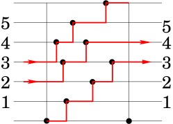
For $\alpha=1/7$ and $N\equiv\pm 3$ mod $7$ there exist two possible entering lines and two leaving lines (cf. Fig. 9)

Figure 9: One of transfer matrix elements for $\alpha=1/7$ and $N\equiv-3$ mod $7$.

The dimension of the transfer matrix in this case is $C_{5}^{2}=10$. Its explicit form is the following

$${\small T(x)=\left(\begin{array}[]{cccccccccc}10p_{6}&35p_{7}&70p_{8}&84p_{9}&56p_{8}&168p_{9}&252p_{10}&210p_{10}&462p_{11}&462p_{12}\\ 10p_{5}&35p_{6}&70p_{7}&84p_{8}&56p_{7}&168p_{8}&252p_{9}&210p_{9}&462p_{10}&462p_{11}\\ 6p_{4}&20p_{5}&40p_{6}&49p_{7}&30p_{6}&91p_{7}&140p_{8}&112p_{8}&252p_{9}&252p_{10}\\ 3p_{3}&8p_{4}&15p_{5}&19p_{6}&10p_{5}&30p_{6}&49p_{7}&35p_{7}&84p_{8}&84p_{9}\\ 4p_{4}&15p_{5}&30p_{6}&35p_{7}&26p_{6}&77p_{7}&112p_{8}&98p_{8}&210p_{9}&210p_{10}\\ 3p_{3}&12p_{4}&25p_{5}&30p_{6}&20p_{5}&61p_{6}&91p_{7}&77p_{7}&168p_{8}&168p_{9}\\ 2p_{2}&6p_{3}&12p_{4}&15p_{5}&8p_{4}&25p_{5}&40p_{6}&30p_{6}&70p_{7}&70p_{8}\\ 0&3p_{3}&8p_{4}&10p_{5}&6p_{4}&20p_{5}&30p_{6}&26p_{6}&56p_{7}&56p_{8}\\ 0&2p_{2}&6p_{3}&8p_{4}&3p_{3}&12p_{4}&20p_{5}&15p_{5}&35p_{6}&35p_{7}\\ 0&0&2p_{2}&3p_{3}&0&3p_{3}&6p_{4}&4p_{4}&10p_{5}&10p_{6}\end{array}\right)\ .}$$ (85)

Finally one obtains that for $\alpha=1/7$ and $N\equiv\pm 3$ mod $7$ the nearest-neighbour distribution for non-symmetric ensemble is

$$p(s) = (a_{2}s^{2}+a_{3}s^{3}+a_{4}s^{4}+a_{5}s^{5}+a_{6}s^{6}+a_{7}s^{7}$$ (86)

$$+a_{8}s^{8}+a_{9}s^{9}+a_{10}s^{10}+a_{11}s^{11}+a_{12}s^{12})\mathrm{e}^{-7s}$$

where $a_{2}\simeq 4.056,\;a_{3}\simeq 28.3898,\;a_{4}\simeq 91.6591,\;a_{5}\simeq 177.9134,\;a_{6}\simeq 227.8782,\;a_{7}\simeq 200.0096,\;a_{8}\simeq 121.6091,\;a_{9}\simeq 50.5880,\;a_{10}\simeq 13.778,\;a_{11}\simeq 2.2159,\;a_{12}\simeq.1596.$

For symmetric matrices under the same conditions

$$p(s) = (a_{1/2}\sqrt{s}+a_{1}s+a_{3/2}s^{3/2}+a_{2}s^{2}+a_{5/2}s^{5/2}+a_{3}s^{3}$$ (87)

$$+ a_{7/2}s^{7/2}+a_{4}s^{4}+a_{9/2}s^{9/2}+a_{5}s^{5}+a_{11/2}s^{11/2})\mathrm{e}^{-7s/2}$$

with $a_{1/2}\simeq.1747,\;a_{1}\simeq.8691,\;a_{3/2}\simeq 2.2565,\;a_{2}\simeq 3.8902,\;$ $a_{5/2}\simeq 4.8085,\;a_{3}\simeq 4.3734,\;a_{7/2}\simeq 2.9327,\;a_{4}\simeq 1.4222,\;$ $a_{9/2}\simeq.4747,\;a_{5}\simeq.0979,\;a_{11/2}\simeq.0094.$

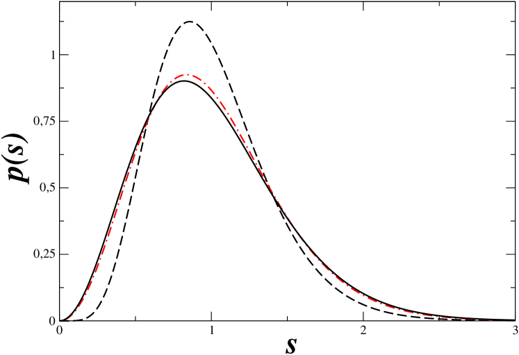
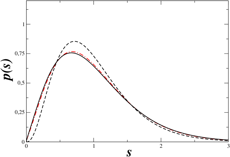
In Fig. 10 and 11 the calculated nearest neighbour distributions are plotted for $\alpha=1/5$ and $\alpha=1/7$ with all possible residues of $N\not\equiv 0$ modulo $1/\alpha$. As expected, the case $N\equiv\pm 1$ mod $1/\alpha$ differs considerably from other cases. When the residue, $k$, increases the nearest-neighbour distribution more and more resembles to the nearest-neighbour distribution of the standard Gaussian ensembles of random matrices. For example, for $\alpha=1/7$ the results with $N\equiv\pm 2$ and $N\equiv\pm 3$ are difficult to distinguish from the Wigner surmise (8) for GUE (for non-symmetric matrices) and for GOE (for symmetric ones)

a)

b)

Figure 10: Nearest-neighbour distribution for $\alpha=1/5$ for (a) the non-symmetric ensemble and (b) the symmetric one. Dashed lines correspond to $N\equiv\pm 1$ mod $5$ given by (13) with $\beta=4$ in (a) and $\beta=3/2$ in (b). Solid lines indicate the results for $N\equiv\pm 2$ mod $5$ given by (80) in (a) and by (81) in (b).

a)

b)

Figure 11: The same as in Fig. 10 but for $\alpha=1/7$. Dashed black lines correspond to $N\equiv\pm 1$ mod $7$ given by (13) with $\beta=6$ in non-symmetric matrices and $\beta=3/2$ for symmetric matrices. The red dotted dashed lines indicate the results for $N\equiv\pm 2$ mod $7$ given by (83) in (a) and by (84) in (b). Solid black lines represent the results for $N\equiv\pm 3$ mod $7$ determined by (86) in (a) and by (87) in (b).

To compare these formulas with the results of numerical simulations it is more precise to use the integrated nearest-neighbour distribution (16). In Figs. 12 and 13 such comparison is performed for all cases considered. The agreement is quite good and the differences are of the same order as in Fig. 2.

a)

b)

Figure 12: Difference between the integrated nearest-neighbour distribution and the corresponding theoretical prediction for $\alpha=1/5$. (a) For non-symmetric ensembles. (b) For symmetric matrices. In each graph pictures differ by the matrix dimensions. From bottom to top $N=801$ ($N\equiv 1$ mod $5$) and $802$ ($N\equiv 2$ mod $5$).

a)

b)

Figure 13: The same as in Fig. 12 but for $\alpha=1/7$. From bottom to top $N=799$ ($N\equiv 1$ mod $7$), $800$ ($N\equiv 2$ mod $7$) , and $801$ ($N\equiv 3$ mod $7$).

7 Summary

A unitary random matrix ensemble

$$M_{kp}=\mathrm{e}^{{\mathrm{i}}\Phi_{k}}\frac{(1-{\rm e}^{2\pi{\rm i}\alpha N})}{N(1-{\rm e}^{2\pi{\rm i}(k-p+\alpha N)/N})}$$ (88)

corresponding to a quantization of a simple pseudo-integrable map (1) is considered in detail. These matrices are characterized by a rational parameter $\alpha=m/q$, the matrix dimension $N$, and symmetry properties of random phases $\Phi_{k}$ (4). To get a well defined limit of the spectral statistics of these ensembles for large $N$ it is necessary to consider increasing sequences of $N$ such that $mN$ has a fixed residue modulo the denominator of $\alpha$

$$mN\equiv k\;\mathrm{mod}\;q$$ (89)

with the residue $k=0,1,\ldots,q-1$. For $k=0$ all eigenvalues of the main matrix can be found analytically as in [14]. For all other residues the spectral statistics of the considered ensembles is non-trivial and differs considerably from standard random matrix ensembles. The cases $k=1$ and $k=q-1$ have been investigated in [15] where it was shown that for these $k$ the nearest-neighbour distribution has the following form

$$p(s)\sim\left\{\begin{array}[]{ll}s^{q-1}\mathrm{e}^{-qs}&\mathrm{for\;non-symmetric\;ensemble}\\ s^{q/2-1}\mathrm{e}^{-qs/2}&\mathrm{for\;symmetric\;ensemble}\end{array}\right..$$ (90)

In the present paper a kind of transfer operator method is developed to calculate the spectral statistics of the same matrix for all values of $k$. It is demonstrated that the nearest-neighbour distribution equals the product of a finite polynomial in $s$ for non-symmetric matrices and in $\sqrt{s}$ for symmetric matrices times the same exponential factor as in (90)

$$p(s)=\left\{\begin{array}[]{ll}\displaystyle\sum_{n=2}^{k(q-k)}a_{n}s^{n}\mathrm{e}^{-qs}&\mathrm{for\;non-symmetric\;ensemble}\\ \displaystyle\sum_{n=1}^{(k(q-k)-1)}a_{n/2}s^{n/2}\mathrm{e}^{-qs/2}&\mathrm{for\;symmetric\;ensemble}\end{array}\right..$$ (91)

Statistical properties of sequences with residue $k$ and $q-k$ are the same. The values of coefficients $a_{n}$ can be calculated by finding the largest eigenvalue and corresponding left and right eigenvectors of the transfer matrix.

For $\alpha=1/5$ and $\alpha=1/7$ and all possible residues the explicit form of these coefficients have been calculated. Numerical simulations in these cases are in a good agreement with obtained formulas. Other correlation functions can also be expressed from the same quantities.

It appears that the considered ensembles of random matrices permit different generalizations which will be discussed elsewhere [19].

Appendix A

The purpose of the Appendix is to give the proofs of certain formulas used in the text.

Let for all $n=1,\ldots,N$

$$\sum_{m=1}^{N}\frac{b_{m}}{x_{m}-y_{n}}=1\;.$$ (92)

Solutions $b_{m}$ of these equations can be expressed in terms of Cauchy determinants and

$$b_{m}=\frac{\displaystyle\prod_{n}(x_{m}-y_{n})}{\displaystyle\prod_{s\neq m}(x_{m}-x_{s})}\;.$$ (93)

A simple way to check it is to consider the function

$$f_{n}(x)=\frac{\displaystyle\prod_{r\neq n}(x-y_{r})}{\displaystyle\prod_{s}(x-x_{s})}=\frac{\displaystyle\prod_{r}(x-y_{r})}{(x-y_{n})\displaystyle\prod_{s}(x-x_{s})}\;.$$ (94)

Asymptotically $f_{n}(x)\to 1/x$ so the integral over a big contour encircling all poles equals 1. Rewriting this integral as the sum poles gives

$$1=\sum_{m}\frac{\displaystyle\prod_{r}(x_{m}-y_{r})}{(x_{m}-y_{n})\displaystyle\prod_{s\neq m}(x_{m}-x_{s})}$$ (95)

which proves (93).

Denote

$$g(x)=\frac{\displaystyle\prod_{n}(x-\Lambda_{n}{\rm e}^{2\pi{\rm i}\alpha})}{x\displaystyle\prod_{k}(x-\Lambda_{k})}\;.$$ (96)

This function decreases as $1/x$ for large $x$ and has poles at $x=0$ and $x=\Lambda_{k}$. Integrating it over a contour encircling all poles one gets

$$1={\rm e}^{2\pi{\rm i}\alpha}+\sum_{m=1}^{N}\frac{\displaystyle\prod_{n}(\Lambda_{m}-\Lambda_{n}{\rm e}^{2\pi{\rm i}\alpha})}{\Lambda_{m}\displaystyle\prod_{k\neq m}(\Lambda_{m}-\Lambda_{k})}$$ (97)

from which it follows that $|B_{m}|^{2}$ defined by (41) obey automatically the normalization condition (33).

References

• [1] M. Berry and M. Tabor, Level clustering in the regular spectrum, Proc. R. Soc. Lond. A 356, 375 (1977)
• [2] O. Bohigas, M.-J. Giannoni, and C. Schmit, Characterization of chaotic quantum spectra and universality of level fluctuation laws, Phys. Rev. Lett. 52, 1 (1984)
• [3] E. Bogomolny, B. Georgeot, M.-J. Giannoni, and C. Schmit, Arithmetical chaos, Phys. Rep. 291, 220 (1997)
• [4] P.J. Richens and M.V. Berry, Pseudointegrable systems in classical and quantum mechanics, Physica D: Nonlinear Phenomena 2, 495 (1981)
• [5] A.N. Zemlyakov and A.B. Katok, Topological transitivity in billiards in polygons, Math. Notes 18, 760 (1975)
• [6] E. Bogomolny, U. Gerland, and C. Schmit, Models of intermediate spectral statistics, Phys. Rev. E 59, R1315 (1999)
• [7] B.I. Shklovskii, B. Shapiro, B.R. Sears, P. Lambrianides, and H.B. Shore, Statistics of spectra of disordered systems near the metal-insulator transition, Phys. Rev. B 47, 11487 (1993)
• [8] F. Evers and A.D. Mirlin, Anderson transitions, Rev. Mod. Phys. 80, 1355 (2008)
• [9] E. Bogomolny, O. Giraud, and C. Schmit, Periodic orbits contribution to the 2-point correlation form factor for pseudo-integrable systems, Commun. Math. Phys. 222, 327 (2001)
• [10] A. Sommerfeld, Optics, Academic Press (1954)
• [11] E. Bogomolny and C. Schmit, Structure of wave functions of pseudointegrable billiards, Phys. Rev. Lett. 92, 244102 (2004)
• [12] E. Bogomolny, B. Dietz, T. Friedrich, M. Miski-Oglu, and A. Richter, Phys. Rev. Lett. 97, 254102 (2006)
• [13] O. Giraud, J. Marklof, and S. O’Keefe, Intermediate statistics in quantum maps, J. Phys. A: Math. Gen. 37, L303 (2004)
• [14] J. Marklof and Z. Rudnick, Quantum unique ergodicity for parabolic map, Geom. Funct. Anal. 10, 1554 (2000)
• [15] E. Bogomolny and C. Schmit, Spectral statistics of a quantum interval-exchange map, Phys. Rev. Lett. 93, 254102 (2004)
• [16] M.L. Mehta, Random Matrices, Academic Press, 2004.
• [17] E. Bogomolny, U. Gerland, and C. Schmit, Short range plasma models for intermediate spectral statistics, Europ. Phys. J. B 19, 121 (2001)
• [18] S. Albeverio, F. Gesztesy, R. Hoegh-Krohn, and H. Holgen, Solvable Models in Quantum Mechanics Springer, New York (1988).
• [19] E. Bogomolny, O. Giraud and C. Schmit, Integrable random matrices, in preparation (2009).
• [20] S. Karlin and J. McGregor, Coincidence probabilities, Pacific J. Math. 9, 1141 (1959)
• [21] M. Martin, O. Giraud, and B. Georgeot, Multifractality and intermediate statistics in quantum maps, Phys. Rev. E. 77, 035201(2008)