Confidence Regions for Means of Random Sets using Oriented Distance Functions

Abstract

Image analysis frequently deals with shape estimation and image reconstruction. The objects of interest in these problems may be thought of as random sets, and one is interested in finding a representative, or expected, set. We consider a definition of set expectation using oriented distance functions and study the properties of the associated empirical set. Conditions are given such that the empirical average is consistent, and a method to calculate a confidence region for the expected set is introduced. The proposed method is applied to both real and simulated data examples.

Keywords: Random Closed Set, Simultaneous Confidence Interval, Image Reconstruction, Shape Estimation.

1 Introduction

Image analysis frequently deals with the problem of shape estimation. Many instances of this may be found, for example, in medical imaging, where shape analysis of brain structures is often used to differentiate between different populations of subjects. Examples include the study of the hippocampus for schizophrenic patients and corpus callosum for adults with fetal alcohol exposure, as well as other neuroanatomical structures (Styner et al., 2004; Bookstein et al., 2002b, a; Styner et al., 2003; Levitt et al., 2009).

To analyze the observed shapes, it is natural to think of them as realizations of random sets. The problem of shape inference then translates into finding the average set and describing its variability.

As the space of closed sets is nonlinear, there is no natural way to define the mean of a set. Indeed, many different definitions of the expected set exist, and therefore one must first select a definition of the mean to work with. Quoting Molchanov (2005), “the definition of the expectation depends on what the objective is, which features of random sets are important to average, and which are possible to neglect”. Here, we focus on the definition of set expectation given in Jankowski and Stanberry (2010), which is based on the oriented distance function (ODF) . The definition is akin to those considered in Baddeley and Molchanov (1998); Lewis et al. (1999), which also rely on the distance function. The ODF definition, however, has several desirable theoretical properties and was found to outperform other definitions in image applications; for a detailed comparison see Jankowski and Stanberry (2010). A thorough review of other existing definitions appears in Molchanov (2005).

In this paper, we study the empirical estimators of the expected set and expected boundary using the ODF definition. We give conditions for consistency of these estimators. We also study their variability using the concept of confidence regions.

Seri and Choirat (2004) present two methods for the calculation of the confidence region of the Aumann expectation. To our best knowledge, this is the only other time confidence regions were studied in the context of random sets. The methodology was developed for convex sets, and therefore the Aumann expectation is a natural choice, as it always yields a convex answer.

Molchanov (1998, Theorem 3.1) gives a central limit theorem for the Hausdorff distance of sublevel sets. Baddeley and Molchanov (1998) use this result to obtain a central limit theorem for their expectation, and this may also be done for the ODF definition. Such central limit theorems could potentially be used to calculate confidence regions. The regions may be found as a dilation of the empirical set estimator. However, this approach requires the estimation of a complex functional of the derivative of the expected distance transform, which renders the method impractical. Furthermore, a dilation approach would provide a uniform confidence region: the distance between the boundary of the mean set and the boundary of the confidence set would be equivalent at all points. Thus, the dilation method would mask important information about the local variability of the estimators.

In this paper, we propose a new and simple approach to calculate confidence regions for both the mean set and its boundary. The method works for both convex and non-convex sets. The resulting confidence regions are conservative in that they cover the expected set with at least $100(1-\alpha)\%$ probability. We show that the confidence regions satisfy certain natural equivariance properties, which are analogous to those of confidence intervals for real–valued parameters. Moreover, the confidence regions provide a simple visual representation of the variability of the estimators and are able to detect local changes in variability. The method can also be used in Bayesian inference to study the behaviour of the posterior sample.

Our definition of the confidence region is based on the quantiles of the supremum of a Gaussian random field. We consider several examples where this quantile is calculated easily. When these quantiles are not available analytically, we propose a bootstrap method to provide approximate confidence regions. The bootstrap approach also avoids making an assumption of an underlying distribution of the observed sets, which could be quite difficult for practitioners.

The outline of this paper is as follows. In Section 2, we review the definitions of set and boundary expectations given in Jankowski and Stanberry (2010). Consistency is studied in Section 3 and the confidence regions are described in Section 4. Section 5 gives several examples of our approach, including a simulation study. We consider the toy image reconstruction example discussed by Baddeley and Molchanov (1998), and analyse the sand grains data first discussed in Stoyan and Molchanov (1997). Lastly, we consider a medical imaging example, and apply our methods to a boundary reconstruction problem in a mammogram image. Proofs and technical details appear in the Appendix, which is available online as supplementary material.

1.1 Notation and Assumptions

Throughout, we let $\mathcal{D}$ denote the domain on which the sets are observed. Unless otherwise stated, we assume that $\mathcal{D}$ is the working domain and write, for example, $A=\{x:x\in A\}$ without stating that $x\in\mathcal{D}$ explicitly. We also assume that $\mathcal{D}$ is a subset of $\mathbb{R}^{d}$, and denote the Euclidean norm of $x$ as $|x|$.

We write $B_{r}(x_{0})=\{x:|x-x_{0}|\leq r\}$ for the closed ball of radius $r$ centered at $x_{0}$. For a set $A$, we write $A^{o},\overline{A},A^{c}$ and $\partial A$ to denote its interior, closure, complement and boundary. Unless noted otherwise, set operations are calculated relative to the domain $\mathcal{D}$. That is, $A^{c}=A^{c}\cap\mathcal{D},$ and so forth. Deterministic sets are denoted using capital letters $A,B\ldots$, while bold upper-case lettering, $\bm{A},\bm{B},\ldots$, is used for random sets.

The notation $C(\mathcal{D})$ is used to denote the space of continuous functions $C(\mathcal{D})=\{f:\mathcal{D}\mapsto\mathbb{R},\ f\mbox{ continuous}\}$ endowed with the uniform topology. That is, $f_{n}\rightarrow f$ in $C(\mathcal{D})$ if $\sup_{x\in K}|f_{n}(x)-f(x)|\rightarrow 0$, for all compact subsets $K\subset\mathcal{D}.$ We write $X_{n}\Rightarrow X$ to say that $X_{n}$ converges weakly to $X$. Throughout the paper, when handling weak convergence of stochastic processes or random fields, we assume that these take values in $C(\mathcal{D})$.

2 Random Closed Set and Its Expectation

Let $\mathcal{F}$ be the family of closed sets of $\mathbb{R}^{d}$ and let $\mathcal{K}$ denote the family of all compact subsets of $\mathbb{R}^{d}$. For a probability triple $(\Omega,\mathcal{A},P)$, a random closed set (RCS) is the mapping $\bm{A}:\Omega\mapsto\mathcal{F}$ such that for every compact set $K\in\mathcal{K}$

$$\{\omega:\bm{A}(\omega)\cap K\neq\emptyset\}\in\mathcal{A}.$$

For more background on random closed sets, we refer to Matheron (1975); Ayala et al. (1991).

2.1 Definition of Expectation

For a nonempty set $A\subset\mathcal{D},$ the distance function is defined as $d_{A}(x)=\inf_{y\in A}|x-y|$ for all $x\in\mathcal{D}.$ Given the distance function of a closed set $A$, the original set may be recovered via $A=\{x:d_{A}(x)=0\}$. Also, the Hausdorff distance may be calculated using the distance function as

$$\rho(A,B) = \max\left\{\sup_{x\in A}d(x,B),\sup_{x\in B}d(x,A)\right\}$$

$$= \sup_{x\in\mathcal{D}}|d_{A}(x)-d_{B}(x)|,$$

for any sets $A,B\subset\mathcal{D}$. We refer to Delfour and Zolésio (2001) for more mathematical properties of the distance function. The distance function has also been used in the context of image thresholding, see for example Friel and Molchanov (1999); Molchanov and Terán (2003).

The oriented distance function (ODF) of any set $A\subset\mathcal{D}$ such that $\partial A\neq 0$ is defined as $b_{A}(x)=d_{A}(x)-d_{A^{c}}(x)$ for all $x\in\mathcal{D}.$ For a closed set, the set and its boundary may now be recovered by $A=\{x:b_{A}(x)\leq 0\}$ and $\partial A=\{x:b_{A}(x)=0\}$. Note that, given only the information at a fixed point $x_{0},$ the ODF is more informative than the distance function. Given the value of $b_{A}(x_{0})$ we know the value of $d_{A}(x_{0}),$ but the converse statement is not true.

For an RCS $\bm{A}$ with a.s. non-empty boundary we define the random function $b_{\bm{A}}(x)$, and denote its pointwise mean as $E[b_{\bm{A}}(x)]$. The mean set and mean boundary are then defined as follows.

Definition 2.1.

Suppose that $\bm{A}$ is a random closed set such that $\partial\bm{A}\neq\emptyset$ almost surely and assume that $E[|b_{\bm{A}}(x_{0})|]<~{}\infty$ for some $x_{0}\in\mathcal{D}$. Then

$$E[\bm{A}] = \{x:E[b_{\bm{A}}(x)]\leq 0\},\hskip 14.22636pt$$

$$\Gamma[\bm{A}] = \{x:E[b_{\bm{A}}(x)]=0\}.$$

Furthermore, we define the expectation of the complement as $E[\bm{A}^{c}]=\{x:E[b_{\bm{A}}(x)]\geq 0\}.$

Remark 2.2.

If $A$ is closed and $\partial A\neq\emptyset$ then $A^{c}$ is open, however, the oriented distance function of $A^{c}$ continues to be well–defined, and indeed we have that $b_{A^{c}}(x)=~{}-~{}b_{A}(x)$. Thus, $E[\bm{A}^{c}]=E\left[\overline{\bm{A}^{c}}\right]=\{x:E[b_{{\bm{A}}}(x)]\geq 0\}$.

Example 1 (disc with random radius).

Suppose that $\bm{A}=\{x:|x|\leq R\}\subset\mathbb{R}^{d}$, for some non–negative, integrable, real-valued random variable $R$. Then $b_{\bm{A}}(x)=|x|-R$ and hence $E[\bm{A}]=\{x:|x|\leq E[R]\}$ and $\Gamma[\bm{A}]=\{x:|x|=E[R]\}$. That is, the expected set is a disc with radius $E[R]$, with boundary equal to the expected boundary.

Example 2 (random singleton).

Suppose that $\bm{A}=\{X\}$ for some $\mathbb{R}^{d}$-valued random variable $X$, then $E[\bm{A}]=\Gamma[\bm{A}]=\emptyset.$

In Example 1, Definition 2.1 yields a natural answer, while the result of Example 2 seems counterintuitive. As mentioned previously, the choice of expectation depends on the problem at hand. The ODF definition was motivated by problems in imaging, where random singletons are regarded as noise. Example 2 illustrates a natural de-noising property of the expectation; see also the discussion in Jankowski and Stanberry (2010).

The function $E[b_{\bm{A}}(x)]$ provides additional information about the mean and its boundary. Recall that $b_{\bm{A}}(x)$ is Lipschitz with constant one almost surely (Delfour and Zolésio, 1994). Therefore, $E[b_{\bm{A}}]$ is also Lipschitz, which also implies that $E[\bm{A}]$ and $\Gamma[\bm{A}]$ are closed sets. Furthermore, if the function $E[b_{\bm{A}}(x)]$ is smooth in a neighbourhood of $x_{0}$, then $\Gamma[\bm{A}]$ is also smooth near $x_{0}.$

Proposition 2.3.

Suppose that $d\geq 2,$ and fix $k\geq 1$, and suppose that the function $E[b_{\bm{A}}(x)]$ is $C^{k}$ in a neighbourhood of $x_{0}$, and that $|\nabla E[b_{\bm{A}}(x_{0})]|\neq 0.$ Then, there exists a (possibly different) neighbourhood of $x_{0}$ such that $\Gamma[\bm{A}]$ is $C^{k}$.

We next consider the estimation of $E[\bm{A}]$ and $\Gamma[\bm{A}].$

Definition 2.4.

Suppose that we observe $\bm{A}_{1},\ldots,\bm{A}_{n}$ random sets, and let

$$\bar{b}_{n}(x)=\frac{1}{n}\sum_{i=1}^{n}b_{\bm{A}_{i}}(x).$$

Then the empirical mean set and the empirical mean boundary are defined as

$$\bar{\bm{A}}_{n}=\{x:\bar{b}_{n}(x)\leq 0\}\ \mbox{ and }\ \overline{\bm{\Gamma}}_{n}=\{x:\bar{b}_{n}(x)=0\}.$$

Similarly to the mean ODF, the function $\bar{b}_{n}$ is Lipschitz, and therefore the empirical sets $\bar{\bm{A}}$ and $\overline{\bm{\Gamma}}_{n}$ are both closed.

2.2 Consistency and Fluctuations of the Empirical ODF

Suppose that we have $n$ independent and identically distributed (IID) RCSs $\bm{A}_{1},\ldots,\bm{A}_{n}$. Then the following results are valid for the average ODF.

Theorem 2.5.

Suppose that $\bm{A}_{1},\ldots,\bm{A}_{n}$ are IID, and that for some $x_{0}\in\mathcal{D}$, $E[b_{\bm{A}}(x_{0})]<\infty.$ Then for all compact subsets $K\subset\mathcal{D}$

$$\lim_{n}\sup_{x\in K}|\bar{b}_{n}(x)-E[b_{\bm{A}}(x)]|=0,$$

almost surely.

Theorem 2.6.

Suppose that $\bm{A}_{1},\ldots,\bm{A}_{n}$ are IID, and that $E[b_{\bm{A}}^{2}(x_{0})]<\infty$ for some $x_{0}\in\mathcal{D}$. Then

$$\mathbb{Z}_{n}(x)\equiv\sqrt{n}(\bar{b}_{n}(x)-E[b_{\bm{A}}(x)])\Rightarrow\mathbb{Z}(x),$$

where $\mathbb{Z}$ is a mean zero Gaussian random field with covariance

$$cov(\mathbb{Z}(x),\mathbb{Z}(y))=E[b_{\bm{A}}(x)b_{\bm{A}}(y)]-E[b_{\bm{A}}(x)]E[b_{\bm{A}}(y)]$$

for $x,y\in\mathcal{D}.$

The next result shows that $\mathbb{Z}$ has very smooth sample paths. Recall that a function $f:\mathbb{R}^{d}\mapsto\mathbb{R}$ is Hölder of order $\alpha$ if it satisfies $|f(x)-f(y)|\leq K|x-y|^{\alpha},$ for some positive finite constant $K$ and $\alpha>0$, for all $x,y$ in the domain of $f$.

Proposition 2.7.

For any $x,y,x^{\prime},y^{\prime}\in\mathcal{D}$

$$\mbox{var}(\mathbb{Z}(x)-\mathbb{Z}(y)) \leq |x-y|^{2},$$ (2.1)

$$|\mbox{cov}(\mathbb{Z}(y)-\mathbb{Z}(x),\mathbb{Z}(y^{\prime})-\mathbb{Z}(x^{\prime}))| \leq 2|y-x||y^{\prime}-x^{\prime}|.$$ (2.2)

Moreover, the sample paths of $\mathbb{Z}$ are Hölder of order $\alpha$, for any $\alpha<1$.

3 Consistency

Here, we study consistency of the estimators $\bar{\bm{A}}_{n}$ and $\overline{\bm{\Gamma}}_{n}$, assuming that $\bar{b}_{n}\rightarrow E[b_{\bm{A}}]$ almost surely in $C(\mathcal{D}).$ By Theorem 2.5, these results apply to IID random closed sets. Following Molchanov (1998), we say that ${\bm{A}}_{n}$ converges strongly to $A$, if the Hausdorff distance $\rho(\bm{A}_{n}\cap K,A\cap K)\rightarrow 0$ almost surely, for any compact set $K$. The following theorem follows from Molchanov (1998, Theorem 2.1) and Cuevas et al. (2006, Theorem 1).

Theorem 3.1.

Suppose that

$$\lim_{n}\sup_{x\in\mathcal{D}}|\bar{b}_{n}(x)-E[b_{\bm{A}}(x)]|=0$$

almost surely, and that $E[\bm{A}]$ is well-defined. Suppose also that the expected ODF, $E[b_{\bm{A}}(x)]$, satisfies

$$\{x:E[b_{\bm{A}}(x)]\leq 0\} = \overline{\{x:E[b_{\bm{A}}(x)]<0\}}.$$ (3.1)

Then $\bar{\bm{A}}_{m}$ converges strongly to $E[{\bm{A}}]$. If $E[b_{\bm{A}}(x)]$ also satisfies

$$\{x:E[b_{\bm{A}}(x)]\geq 0\} = \overline{\{x:E[b_{\bm{A}}(x)]>0\}},$$ (3.2)

then $\overline{\bm{\Gamma}}_{n}$ converges strongly to $\Gamma[{\bm{A}}]$.

Condition (3.1) says that the expected ODF is not allowed to have a local minimum on $\Gamma[\bm{A}]=\{x:E[b_{\bm{A}}(x)]=0\}$, while (3.2) excludes mean ODFs which have a local maximum on $\Gamma[\bm{A}]$ (again, this need not be unique). Alternatively, since $E[b_{\bm{A}}(x)]$ is a continuous, condition (3.1) says that $E[\bm{A}]$ is a topologically regular closed set, while condition (3.2) says that $E[\bm{A}^{c}]$ is a topologically regular open set.

Remark 3.2.

It is possible that $E[b_{\bm{A}}(x)]$ violates the conditions (3.1) and/or (3.2) and consistency still holds. For example, consider the RCS ${\bm{A}}=\{x_{0}\}\subset\mathbb{R}^{d}$ almost surely. Then IID sampling trivially produces a consistent estimate, but $E[b_{\bm{A}}(x)]$ fails to satisfy (3.1).

Example 3 (half plane).

For $\mathcal{D}\subset\mathbb{R}^{d}$, consider the RCS ${\bm{A}}=\{x\in\mathcal{D}:x_{1}\leq\Theta\}$, where $\Theta$ is a real-valued random variable with finite mean $E[\Theta].$ Then $b_{\bm{A}}(x)=x_{1}-\Theta$, and $E[b_{\bm{A}}(x)]=x_{1}-E[\Theta].$ The mean ODF satisfies both conditions (3.1) and (3.2), and therefore $\bar{\bm{A}}_{n}=\{x:x_{1}\leq\bar{\Theta}_{n}\}$ and $\overline{\bm{\Gamma}}_{n}=\{x:x_{1}=\bar{\Theta}_{n}\}$ are consistent estimators of $E[{\bm{A}}]=\{x:x_{1}\leq E[\Theta]\}$ and $\Gamma[{\bm{A}}]=\{x:x_{1}=E[\Theta]\}$. Indeed, we may easily check that $\rho(E[{\bm{A}}],\bar{\bm{A}}_{n})=\rho(\Gamma[{\bm{A}}],\overline{\bm{\Gamma}}_{n})=|\bar{\Theta}_{n}-E[\Theta]|$ which converges to zero almost surely.

The following result provides some further insight into the consistency conditions.

Proposition 3.3.

Conditions (3.1) and (3.2) may be re–written in terms of mean set properties.

1. Condition (3.1) holds iff $\partial E[\bm{A}^{c}]=\Gamma[\bm{A}],$ and iff $E[{\bm{A}}]=\overline{(E[{\bm{A}}^{c}])^{c}}.$

2. Condition (3.2) holds iff $\partial E[\bm{A}]=\Gamma[\bm{A}]$, and iff $E[{\bm{A}}^{c}]=\overline{(E[{\bm{A}}])^{c}}.$

Example 4 (set and its boundary).

Suppose that ${\bm{A}}\subset\mathbb{R}$ is either $[0,1]$ or $\{0,1\}$ with equal probability. Then $E[{\bm{A}}]=\Gamma[{\bm{A}}]=[0,1]$, while $E[\bm{A}^{c}]=\mathbb{R}$. On the other hand, if $[0,1]$ is seen with probability $p$, then if $p<0.5$, we have that $E[{\bm{A}}]=\Gamma[{\bm{A}}]=\{0,1\}$; If $p>0.5$, then $E[{\bm{A}}]=[0,1]$ and $\Gamma[{\bm{A}}]=\{0,1\}.$ The case $p=0.5$ provides a setting where neither (3.1) nor (3.2) are satisfied.

We observe $n$ independent sets ${\bm{A}}_{1},{\bm{A}}_{2},\ldots,{\bm{A}}_{n}$, where each $\bm{A}_{i}$ is either $[0,1]$ or $\{0,1\}$ with equal probability. Let $\widehat{p}_{n}$ denote the proportion of the random sets equal to $[0,1]$. Then

$$\bar{b}_{n}(x)=\widehat{p}_{n}b_{[0,1]}(x)+(1-\widehat{p}_{n})b_{\{0,1\}}(x),$$

and it follows that whenever $\widehat{p}_{n}<0.5$, $\bar{\bm{A}}_{n}=\overline{\bm{\Gamma}}_{n}=\{0,1\}$, and for $\widehat{p}_{n}>0.5$, $\bar{\bm{A}}_{n}=[0,1]$ while $\overline{\bm{\Gamma}}_{n}=\{0,1\}$. Clearly, convergence to the expected set or the expected boundary can never be achieved.

Example 5 (missing centre).

Suppose that $\bm{A}$ is either a disc or an annulus in $\mathbb{R}^{2}$; that is,

$$\bm{A} = \left\{\begin{array}[]{ll}\{x:|x|\leq 1\}&\mbox{with probability $p$},\\ \{x:0.5\leq|x|\leq 1\}&\mbox{otherwise.}\end{array}\right.$$

Then the expected set $E[{\bm{A}}]$ is an annulus for $p<1/3$, and a disc for $p\geq 1/3$. For $p\neq 1/3$, the expected ODF satisfies both (3.1) and (3.2). For $p=1/3,$ we have

$$E[b_{A}(x)] = \left\{\begin{array}[]{ll}|x|-1&\mbox{for }|x|\geq 0.75,\\ -|x|/3&\mbox{otherwise,}\end{array}\right.$$

and hence $E[\bm{A}]=\{x:|x|\leq 1\}$ while $\Gamma[\bm{A}]=\{x:|x|=0,1\}\neq\partial E[\bm{A}]$. Since $E[b_{\bm{A}}(x)]$ has a local maximum at $x=0$, it fails to satisfy (3.2), and therefore this point may be omitted by the estimators $\overline{\bm{\Gamma}}_{n}$.

Figure 1: The expected boundary (white) for Example 6 is superimposed on a grey scale image of the expected ODF.

Example 6 (blinking square).

Suppose that the RCS ${\bm{A}}$ is either a rectangle or a union of two squares with equal probability. Specifically, define

$$A_{1} = \{x:0\leq x_{1}\leq 3,0\leq x_{2}\leq 1\},$$

$$A_{2} = \{x:0\leq x_{1}\leq 1,0\leq x_{2}\leq 1\}\cup\{x:2\leq x_{1}\leq 3,0\leq x_{2}\leq 1\}.$$

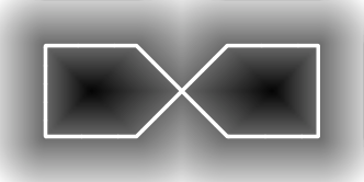
Then $\bm{A}=A_{1}$ with probability 0.5, and otherwise $\bm{A}=A_{2}.$ Thus, half of the time the $\bm{A}$ has its “middle” removed. The resulting mean set and mean boundary are shown in Figure 1. Here, the expected ODF has no local maxima, or minima, along the boundary, and therefore both (3.1) and (3.2) are satisfied.

4 Confidence Regions

We now construct confidence regions, or confidence supersets, for both $E[{\bm{A}}]$ and $\Gamma[{\bm{A}}].$ To do this, we assume that the sets are observed on a compact window $\mathcal{W}\subseteq\mathcal{D}$. We also assume that $\mathbb{Z}_{n}\Rightarrow\mathbb{Z}$ in $C(\mathcal{W}),$ which holds, for example, under IID sampling by Theorem 2.6.

Definition 4.1.

Let $q_{1}$ and $q_{2}$ be numbers such that $\mbox{pr}(\sup_{x\in\mathcal{W}}\mathbb{Z}(x)\leq q_{1})=1-\alpha$, and $\mbox{pr}(\sup_{x\in\mathcal{W}}|\mathbb{Z}(x)|\leq q_{2})=1-\alpha$. Then, a $100(1-\alpha)\%$ confidence region for $E[{\bm{A}}]\cap\mathcal{W}$ is

$$\left\{x\in\mathcal{W}:\bar{b}_{n}(x)\leq q_{1}/\sqrt{n}\right\}$$ (4.1)

and a $100(1-\alpha)\%$ confidence region for $\Gamma[{\bm{A}}]\cap\mathcal{W}$ is

$$\left\{x\in\mathcal{W}:|\bar{b}_{n}(x)|\leq q_{2}/{\sqrt{n}}\right\}.$$ (4.2)

By Proposition 2.7, the limiting field $\mathbb{Z}$ is continuous, and therefore both $\sup_{x\in\mathcal{W}}\mathbb{Z}(x)$ and $\sup_{x\in\mathcal{W}}|\mathbb{Z}(x)|$ are well-defined. Further, Proposition 2.7 gives a uniform upper bound on the variability of the increments of the random field. Understanding the path properties of the process $\mathbb{Z}$, such as smoothness, provides information about the variability of the quantiles $q_{1}$ and $q_{2}$ and therefore also on the tightness of the confidence sets. We also make the following comments about the new definition.

• The confidence region is conservative, in that it covers the set $E[{\bm{A}}]\cap\mathcal{W}$ or $\Gamma[{\bm{A}}]\cap\mathcal{W}$ with a probability of at least $100(1-\alpha)\%.$ One reason why the method is conservative is our use of the supremum of the fluctuation field to find the cut–off quantile values. However, the field $\mathbb{Z}$ is very smooth and highly correlated by Proposition 2.7. Therefore, we expect that the proposed method, although conservative, yields reasonable answers, especially for sets that have been co–registered apriori. We explore the question of over–coverage via simulations in Section 5.2.

• The confidence region is “immune” to the consistency conditions (3.1) and (3.2); see Example 8.

• If the exact distribution of $\mathbb{Z}$ is unknown (as is often the case in practice), the quantiles may be approximated using a bootstrap approach. For computational reasons, it is often easier to calculate asymmetric quantiles in (4.2).

• The confidence region gives no information as to the geometry of the random sets. That is, the shape of the confidence region may be similar for observed random sets which are stars, as well as for those which are squares.

Figure 2: Confidence regions for Example 7: (left) the mean boundary $\Gamma[{\bm{A}}]$ in black and the empirical boundary $\overline{\bm{\Gamma}}_{n}$ in grey; (centre) a 95% bootstrap confidence set for $E[\bm{A}]$; (right) a 95% bootstrap confidence set for $\Gamma[\bm{A}]$. The expected boundary $\Gamma[\bm{A}]$ is shown in black for comparison.

Example 7 (disc in $\mathbb{R}^{2}$ with random centre).

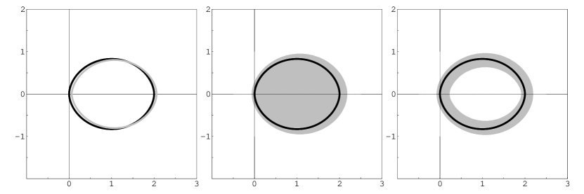
The random set is a disc with radius one centred at $(\Theta,0)$ where $\Theta$ is Uniform$[0,2]$, and suppose that we observe 100 IID random sets from this model. The expected set $E[\bm{A}]$ is shown in Figure 2. Moreover, since $E[b_{\bm{A}}(x)]\geq|x-x_{0}|-1$ where $x_{0}=(E[\Theta],0)$, it follows that $E[\bm{A}]$ is contained inside the disc of radius one centered at $(1,0)$. Confidence regions were formed for both $\Gamma[{\bm{A}}]$ and $E[{\bm{A}}]$ using re-sampling techniques to estimate the quantiles of $\sup_{x\in\mathcal{W}}\mathbb{Z}(x)$ and $\sup_{x\in\mathcal{W}}|\mathbb{Z}(x)|$ where the window $\mathcal{W}=[-2,2]\times[-1,3].$ These are illustrated in Figure 2.

Example 8 (confidence regions for the set and its boundary).

Let $[0,1]\subset\mathbb{R}$ and suppose that $\bm{A}$ is either $\{0,1\}$ or $[0,1]$ with equal probability. Suppose also that we observe a simple random sample of size $n$ from this model. Recall that $E[{\bm{A}}]=\Gamma[{\bm{A}}]=[0,1]$, and $E[b_{\bm{A}}(x)]$ satisfies neither (3.1) nor (3.2). As before, let $\widehat{p}_{n}$ denote the proportion of times that the set $[0,1]$ is observed. If $\widehat{p}_{n}>0.5$, then $\bar{\bm{A}}_{n}=\overline{\bm{\Gamma}}_{n}=\{0,1\}\neq[0,1]$. If $\widehat{p}_{n}<0.5$, then $\bar{\bm{A}}_{n}=[0,1]$ with $\overline{\bm{\Gamma}}_{n}=\{0,1\}\neq\Gamma[{\bm{A}}].$

The fluctuation field is given by

$$\mathbb{Z}_{n}(x) = \sqrt{n}(\widehat{p}_{n}-0.5)\left(b_{[0,1]}(x)-b_{\{0,1\}}(x)\right)$$

$$\Rightarrow Z\left(b_{[0,1]}(x)-b_{\{0,1\}}(x)\right),$$

where $Z$ is a univariate normal random variable with mean zero and variance $0.25$. The largest difference for $b_{[0,1]}(x)-b_{\{0,1\}}(x)$ occurs at $x=0.5$, and hence, for any window such that $[0,1]\subset\mathcal{W}$, we have

$$\sup_{x\in\mathcal{W}}\mathbb{Z}(x)=\max\{-Z,0\},\ \ \ \mbox{and }\ \sup_{x\in\mathcal{W}}|\mathbb{Z}(x)|=|Z|.$$

Therefore, the exact quantiles are $q_{1}=1.645/2$ and $q_{2}=1.96/2$, and the confidence region for $\Gamma[{\bm{A}}]$ is given by $\{x:|\bar{b}_{n}(x)|\leq 1.96/2\sqrt{n}\}.$ Now, for any $n$, $\max_{x\in[0,1]}|\bar{b}_{n}(x)|=|\bar{b}_{n}(0.5)|=|0.5-\widehat{p}_{n}|$. Therefore the confidence region misses a part of $\Gamma[{\bm{A}}]$ if and only if $|0.5-\widehat{p}_{n}|>1.96/2\sqrt{n}$. For large $n$, this happens with a probability of roughly $0.95$. On the other hand, the Hausdorff distance $\rho(\Gamma[\bm{A}],\overline{\bm{\Gamma}}_{n})=0.5$ whenever $\widehat{p}_{n}\neq 0.5.$ This example illustrates that the confidence regions are not affected by the violation of the consistency conditions.

Example 9 (confidence set for disc with random radius).

Suppose that $\bm{A}$ is a disc with random radius $R$ with $\mu=E[R]$ and $\sigma^{2}=\mbox{var}(R)$. Then the expected set is a circle with radius $\mu$. Also, the 95% confidence interval for $E[{\bm{A}}]$ is a circle with radius $\mu+1.645\sigma/\sqrt{n}$, while the 95% confidence set for $\Gamma[{\bm{A}}]$ is the band $\{x:\mu-1.96\sigma/\sqrt{n}\leq|x|\leq\mu+1.96\sigma/\sqrt{n}\}$.

Figure 3: Left: the expected boundary $\Gamma[{\bm{A}}]$ (black), its estimate based on 25 samples (grey) and the boundary of a pacman with radius 0.5 (dashed); centre and right: 95% bootstrapped confidence regions for $E[\bm{A}]$ and $\Gamma[\bm{A}]$, respectively. The confidence sets are denoted by the shaded area, while the black line shows $\Gamma[\bm{A}]$.

Example 10 (pacman in $\mathbb{R}^{2}$).

Define the pacman with radius $r$, $A(r)$, to be a disc with radius $r$ centred at the origin with its upper left quadrant removed. That is,

$$A(r)=\{x:|x|\leq r\}\cap\left\{\{x:x_{1}\leq 0\}\cup\{x:x_{2}\leq 0\}\right\}.$$

Figure 3 (right, dashed) shows the contour of $A(r)$ for $r=0.5$. Suppose that $\bm{A}=\bm{A}(R),$ where $R$ is a uniform random variable on $[0,1].$

The expected set $E[\bm{A}]$ is a smoothed version of $A(0.5)$, as seen in Figure 3 (left). Recall that the smoothness of the boundary depends on the smoothness of $E[b_{\bm{A}}(x)]$. As the latter is an integral, which tends to have more smoothness than the original function, we expect that in general the expectation is as or more smooth than the original realizations of the boundary. This is exactly what one sees in Figure 3: the mean boundary is smoothed out in the regions where there is movement; however, since the origin is a fixed point of the random boundary, no additional smoothness is introduced here by the average.

Figure 3 also shows bootstrapped $95\%$ confidence sets for both $E[{\bm{A}}]$ and $\Gamma[{\bm{A}}].$ The accuracy of the estimate and the apparent centering of the confidence intervals around the mean set may be explained upon closer inspection of the sample. The ODF of the pacman is similar to that of the circle; indeed, they are identical in the lower left quadrant. Therefore, the behaviour of the estimators and of the confidence regions is not unlike that of estimators and confidence intervals for the real-valued $E[R]=0.5$. For our sample of $n=25$, we observed $\bar{R}_{n}=0.496,$ which explains the accuracy of the estimator $\overline{\bm{\Gamma}}_{n}$. On the other hand, the confidence region still shows the large variability of $\overline{\bm{\Gamma}}_{n}$.

RCS with simplified ODF structure.

Consider an RCS $\bm{A}$ and suppose that there exist functions $h_{j}$ $j=1,\ldots,k$ and random variables $\eta_{j}$ $j=1,\ldots,k$ such that

$$b_{\bm{A}}(x)=\sum_{j=1}^{k}h_{j}(x)\,\eta_{j}$$

for all $x\in\mathcal{D}$ (see also Section 3 in Jankowski and Stanberry (2010)). For example, the ball centered at $x_{0}$ with random radius $R$ takes this form. Here, $b_{\bm{A}}(x)=|x-x_{0}|-R$, and hence $h_{1}(x)=|x-x_{0}|,h_{2}(x)=-1$ and $\eta_{1}=1,\eta_{2}=R.$

For such sets, both the empirical and ODF average have a similar simplified form. That is, $\bar{b}_{n}=\sum_{j=1}^{k}h_{j}(x)\,\bar{\eta}_{n,j}$ and $E[b_{\bm{A}}(x)]=\sum_{j=1}^{k}h_{j}(x)\,E[\eta_{j}].$ Furthermore, the fluctuation field for these sets is particularly straightforward. Suppose that we observe IID samples of the random vector $(\eta_{1},\ldots,\eta_{k})$, and assume that $E[\eta_{j}^{2}]<\infty$ for all $j=1,\ldots,k$. Then

$$\mathbb{Z}_{n}(x)\Rightarrow\sum_{j=1}^{k}Z_{j}h_{j}(x),$$

where $Z=\{Z_{1},\ldots,Z_{k}\}$ is a multivariate normal random variable with mean zero and variance matrix given by $\mbox{cov}(Z_{j},Z_{m})=\mbox{cov}(\eta_{j},\eta_{m}).$

Example 11 (Random half-plane).

Suppose that $\Theta\sim$Uniform$[a,b]$ and let $\bm{A}=\{x:x_{2}\geq x_{1}\tan\Theta\}.$ That is, $\bm{A}$ is the plane above the line which goes through the origin and has angle $\Theta$ with the $x_{1}$-axis. Here, $b_{\bm{A}}(x)=x_{1}\sin\Theta-x_{2}\cos\Theta,$ and hence $h_{1}(x)=x_{1},h_{2}(x)=x_{2}$ and $\eta_{1}=\sin\Theta,\eta_{2}=\cos\Theta.$ Some calculations also reveal that $E[\bm{A}]=\{x:x_{2}\geq x_{1}\tan((a+b)/2)\}$ and $\Gamma[\bm{A}]=\{x:x_{2}=x_{1}\tan((a+b)/2)\}.$

The confidence region for $\Gamma[\bm{A}]$ is a strip centred on the line $x_{2}=x_{1}\bar{\eta}_{1}/\bar{\eta}_{2}$ of width $q_{2}/\sqrt{n}\,\bar{\eta}_{2},$ where $q_{2}$ is the $1-\alpha$ quantile of $\sup_{x\in D}|Z_{1}x_{1}+Z_{2}x_{2}|.$

4.1 Equivariance Properties

The following proposition gives equivariance properties of the confidence regions under dilation and rigid motion. The result corresponds to the classical scaling results for the mean and standard deviation of univariate data.

Proposition 4.2.

Consider a random closed set $\bm{A}\subset\mathcal{D}.$ Let $\bm{C}$ and $\bm{C}_{\Gamma}$ denote the confidence regions for $E[\bm{A}]\cap\mathcal{W}$ and $\Gamma[\bm{A}]\cap\mathcal{W},$ respectively.

1. Fix $\alpha>0$, and let $\bm{A}_{1}=\alpha\bm{A}$ with $\mathcal{W}_{1}=\alpha\mathcal{W}.$ Then the confidence regions for $E[\bm{A}_{1}]\cap\mathcal{W}_{1}$ and $\Gamma[\bm{A}_{1}]\cap\mathcal{W}_{1}$ are $\alpha\bm{C}$ and $\alpha\bm{C}_{\Gamma},$ respectively.

2. Fix a rigid motion $g\in E(d)$, and let $\bm{A}_{2}=g(\bm{A})$ with $\mathcal{W}_{2}=g(\mathcal{W}).$ Then the confidence regions for $E[\bm{A}_{2}]\cap\mathcal{W}_{2}$ and $\Gamma[\bm{A}_{2}]\cap\mathcal{W}_{2}$ are $g(\bm{C})$ and $g(\bm{C}_{\Gamma}),$ respectively.

4.2 A Modified Approach

It is not hard to see that the variability of $\bar{\bm{A}}_{n}$ and $\overline{\bm{\Gamma}}_{n}$ depends on the local fluctuations of the field $\mathbb{Z}$ around $\Gamma[\bm{A}]$ (see also Molchanov (1998, Theorem 3.1)). One natural way to incorporate this idea into calculation of the confidence region is described below.

1. Calculate the $100(1-\alpha)\%$ confidence regions for $\Gamma[\bm{A}]$ as described in the previous section. Let $C$ denote this region.

2. Find the $100(1-\alpha/2)\%$ upper quantile of $\sup_{x\in C}|\mathbb{Z}(x)|$, and call this $\tilde{q}_{2}$.

3. The $100(1-\alpha)\%$ confidence region for $\Gamma[\bm{A}]$ is then calculated as $\left\{x:|\bar{b}_{n}(x)|\leq\tilde{q}_{2}/\sqrt{n}\right\}.$

The modification is designed to decrease the size of the quantile $q_{1}$ in (4.1). In the first step we reduce the size of the domain of the supremum to a set which is likely to contain the boundary. Note also that the set $C$, and therefore also $\tilde{q}_{2},$ depend on the sample size $n$. Thus, the larger the sample size, the more effective the modification. A similar approach yields a modified confidence region for $E[\bm{A}].$ We find that this modification yields a slight improvement in the coverage probabilities for some settings, although visually the confidence regions remain quite similar. Notably, iterating (i)–(iii) does not improve the size of the region or the coverage probabilities.

5 Examples

5.1 Implementation

There exist several efficient algorithms to calculate the distance function of any set, which allows for easy implementation of our methods (Breu et al., 1995; Freidman et al., 1977; Rosenfeld and Pfaltz, 1966). For many of the examples presented here, the oriented distance function may be calculated exactly. When this was not possible, our calculations were implemented in MATLAB (MathWorks), where the bwdist command was used to compute the oriented distance function of a set. Here, the examples need to be discretized to pixels (in $\mathbb{R}^{2}$) or voxels (in $\mathbb{R}^{3}$). This discretization introduces an additional source of error; see Serra (1984) for a thorough treatment of the induced difficulties.

To minimize the effect of discretization, in the simulations described below, we selected a fine gird, which was calibrated to give accurate results. Suppose that $\mathcal{D}\subset\mathbb{R}^{2}$, and that we observe $n$ discs centered at the origin with random radius $U\sim$Uniform[0,1]. Here, the confidence regions for the mean boundary are exact (modulo the sample size approximations). Setting $n=1000$, we obtained empirical coverage probabilities of 95.10, 95.02, 95.30, 95.30, and 94.96 for the 95% confidence regions, for grids with side length $m=200,400,600,800,1000$, respectively (the standard error due to bootstrap sampling was 0.0031). Finally, we selected $m=400$ for our simulations.

5.2 Simulation Study

Table 1: Empirical coverage probabilities for the expected set / expected boundary.

	$n=25$		$n=100$
$100(1-\alpha)\%$	$90\%$	95%	90%	95%
(A)	88.40/89.65	94.76/95.60	90.40/91.23	95.68/94.12
(B)	90.24/89.85	94.63/95.05	90.16/90.35	95.14/95.04
(C1)	90.07/91.15	94.36/95.10	91.64/91.05	95.28/95.29
(C2)	91.39/93.49	96.45/97.37	92.14/93.31	96.85/97.13
(D1)	91.99/90.98	96.32/95.73	91.81/91.70	96.20/95.74
(D2)	90.67/88.56	94.48/94.66	90.95/88.89	94.86/94.97

We next simulate coverage probabilities for several examples of random closed set models. The particular examples we consider are given below.

1. The set and its boundary when $p=0.5$, considered in Example 4. Recall that in this example netiher the set estimator nor the boundary estimator is consistent. Here $\mathcal{W}=[-1,2].$

2. The pacman with random radius $R\sim$Uniform[0,2] (see Example 10). Here $\mathcal{W}=[-2,2]^{2}.$ Although the pacman RCS is not decomposable, it still exhibits similar behaviour.

3. The random set $\bm{A}=\bm{A}_{1}\cup\bm{A}_{2},$ where $\bm{A}_{1}$ and $\bm{A}_{2}$ are both random discs. The two cases we consider are as follows.

   1. $\bm{A}_{1}$ is centered at the origin and has radius $R_{1}\sim$Uniform[0,2]. $\bm{A}_{2}$ is centered at the point $(3,0)$ and has radius $R_{2}\sim$Uniform[0,1]. Here $\mathcal{W}=[-2,4]\times[-2,2].$

   2. $\bm{A}_{1}$ is centered at the origin and has radius $R_{1}\sim$Uniform[0,1]. $\bm{A}_{2}$ is centered at the point $(1,0)$ and has radius $R_{2}\sim$Uniform[0,1]. Here $\mathcal{W}=[-1,2]\times[-1,1].$ The mean set and some sample sets are shown in Figure 4.

4. A random ellipse with boundary parameterized as $(x_{1}/R_{1})^{2}+(x_{2}/R_{2})^{2}=1$. Let $U_{1},U_{2}$ be two independent random variables with distribution Uniform$[0,1].$ The two cases we consider are as follows. Throughout, we assume that $\mathcal{W}=[-1.5,1.5]\times[-1,1].$

   1. $R_{1}=1,R_{2}=0.5+U_{2}/2$.

   2. $R_{1}=1+U_{1}/5,R_{2}=0.5+U_{2}/2$.

In the above examples, the image was discretized and the quantiles were estimated using Monte Carlo methods (with $B=2000$ repetitions and $n=100$), except for example (A), where the quantile is known exactly. The empirical coverage was estimated using $10,000$ Monte Carlo simulations in each case. It is important to note that there are four sources of error: sample size, discretization, the bootstrap estimation of the quantile, and the Monte Carlo simulations themselves. The maximal standard error due to Monte Carlo of the empirical coverage probabilities is $0.30\%$, but it is not easy to quantify the standard error due to the other three sources. In particular, we note that the quantile was estimated once per example, and the same quantile was used in each Monte Carlo simulation (otherwise, the simulations would have been prohibitive), which increases the bias of our results.

Figure 4: The mean set in Example (C2) in white on a gray background. The boundaries of several sample sets are also shown.

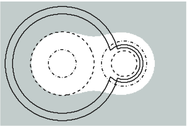
The results of the simulation study show that our methods, though conservative, achieve good coverage probabilities. The greatest over-coverage is seen in Example (C2), which is the most difficult of the examples because the observed sets have not been co-registered; see Figure 4 for some sample sets. In this example, it is possible that a slight improvement of the coverage probability could be seen by a modification to the confidence region discussed in Section 4.2. In general, to minimise over-coverage, we recommend choosing $\mathcal{W}$ as small as possible in practice.

5.3 A Toy Image Reconstruction Example

Figure 5: A sample reconstructed image (left) and ODF average based on 15 IID samples from the posterior (right).

Image averaging arises in various situations, for example, when multiple images of the same scene are observed or when the acquired images represent objects of the same class and the goal is to determine the average object (shape) that can be described as typical. Here we consider an example of image averaging studied in Baddeley and Molchanov (1998). The data set consists of 15 independent samples of a reconstructed newspaper image (Figure 5, left), and is available from http://school.maths.uwa.edu.au/homepages/adrian. For details on how the data was generated we refer to Baddeley and Molchanov (1998).

Figure 6: 95% confidence regions for $E[\bm{A}]$ (left) and $\Gamma[\bm{A}]$ (right). The boundary of the original newspaper image is shown in black.

The empirical average of the 15 observed images, $\bar{\bm{A}}_{n}$ is shown in Figure 5 (right). The average $\bar{\bm{A}}_{n}$ describes the “typical” image reconstruction, and as such, may be thought of as an estimator of the true text image. Next, we compute 95% confidence regions for the ODF-average reconstruction based on 5K bootstrap samples. We may think of these regions as a measure of the variability of $\bar{\bm{A}}_{n}$, and $\overline{\bm{\Gamma}}_{n}$. Figure 6 (top) shows the confidence region for $E[\bm{A}]$ with the boundary of the true image overlayed in black. The confidence set contains all of the true text image and appears tight, although there are a number of spurious bounds induced by noise. The confidence set for $\Gamma[\bm{A}]$ is also shown in Figure 6 (right). The boundary of the lower confidence set consists of only a few closed contours scattered throughout the text. The lack of tightness in the confidence set is explained by the small sample size and a relatively thin font width. Hypothetically increasing the sample size would produce tighter confidence sets for both the expected set and its boundary. For example, the bootstrap confidence set for the boundary based on 50 and 100 samples is tighter as compared to the one based on 15 samples (see Figure 7). We expect that actual confidence regions for $n=50$ and $n=100$ would exhibit even less noise than the hypothetical regions shown in Figure 7. It should be noted that the confidence regions in Figure 7 were created using the original window $\mathcal{D}$, and the picture is a close-up of the result.

Figure 7: Confidence regions for the expected boundary with the boundary of the true image (black) using the true sample size (left) and hypothetical sample sizes of $n=50,100$ (middle and right, respectively). The pictures shown are insets of the full image.

Note that these images were generated under a Bayesian framework, where the goal is to reconstruct the original image by selecting an appropriate parameter from the posterior distribution. Here, this parameter is not computable directly, and is instead estimated by $\bar{\bm{A}}_{n}$ and $\overline{\bm{\Gamma}}_{n}$. Although a frequentist concept, the confidence regions allow us to determine the variability of these estimators. As Figure 7 shows, this variability depends on the sample size.

5.4 Analysis of Sand Grains

         

         

Figure 8: Confidence regions (grey) for the average grain (top row) and the average boundary (bottom row) from the Zelenchuk river (left column) and the Baltic Sea (right column), based on realignment with scaling.

Next, we apply the proposed methods to the sand grains data previously described in Stoyan and Molchanov (1997) and Kent et al. (2000). The sand particles were collected from the shores of the Baltic Sea and banks of the Zelenchuk River in Ossetia. The grains were photographed on the same scale and the data resembles two dimensional projections represented by binary images. Both images may be found online at www.math.yorku.ca
/$\sim$hkj/Research/SandGrains (please note that the online images are not to scale). The observed sand grains generally have a smooth rounded shape, but are not necessarily covex.

The grains from the two regions appear to differ both in shape and size with sea grains being more spherical and larger as compared to river grains that are more oblong and smaller in diameter. To summarize the data, we find the average grains and their average boundaries for each group. We also construct confidence regions to describe the variability of the grain shapes.

         

         

Figure 9: Confidence regions (grey) for the average grain (top row) and the average boundary (bottom row) from the Zelenchuk river (left column) and the Baltic Sea (right column), based on realignment without scaling.

To begin with, the particles were realigned using the generalised Procrustes analysis as implemented in the shapes package in R (R Development Core Team, 2009). To apply the Procrustes analysis, we use the digitized data as described by Kent et al. (2000). The data was digitized so that each sand grain was represented by 50 vertices approximately equally spaced on the boundary. After digitization, the arc-length between the vertices is around 10-20 pixels with grain particles represented by high-resolution images of size $500\times 350$. The realignment was done with and without scaling. Using the scaling, we essentially remove the size effect and can examine differences in average shapes. Alternatively, average particles based on Procrustes analysis without scaling reflect differences both in size and shapes of the particles. The median (IQR) centroid sizes are 1481 (1396, 1665) and 2076 (1867, 2376) for the river and sea grains, respectively, indicating the sea particles to be bigger as compared to the river ones.

Figure 8 shows the confidence regions for the average particle (top row) and the expected boundary (bottom row) for the river (left column) and the sea (right column) sands using scaled realignment. White contours show the empirical mean boundary. The confidence regions are based on 5K bootstrap samples. The average river grain is more oblong as compared to the sea grain. The variability within the two groups appears to be rather similar. Figure 9 shows the confidence regions for the average particle (top row) and the expected boundary (bottom row) for the river (left column) and the sea (right column) sands, based on realignment without scaling. White contours show the empirical mean boundary. The confidence regions are based on 5K bootstrap samples. The average sea grain is more spherical in shape as compared to the river average. It is also considerably larger in size. The variability within the two groups again appears to be rather similar, however, the unscaled images appear more variable than the scaled ones. Overall, the discrepancies in shape and size between the two averages reflect the differences between the raw data sets. Note that the boundaries of the average sets in both figures are rather smooth.

There is also a marked difference between the scaled and unscaled river sand grain averages. Image results from the Procrustes analysis re–alignment with and without re–scaling are quite different. This is to be expected, as the scaling, location, and centering re–alignments in Procrustes analysis are highly interdependent. It would be of interest to compare other re–alignment methods, such as those proposed by Stoyan and Molchanov (1997), but this is beyond the scope of this work.

Whether or not scaled Procrustes realignment is applied, the averages of the particles show a clear difference between the two groups. However, this difference is at this time only visual. An interesting and important problem is to develop quantifiable methodology to test for presence and locations of differences between the mean shapes.

5.5 Application to Medical Imaging

Figure 10: Confidence sets for the reconstructed skin-air boundary in a mammogram: the original image (left), and the digitally enhanced image (centre) with the reconstructed boundary (solid line) and confidence region (dashed line). Three insets are also shown (right).

We next consider an example of boundary reconstruction in mammography, where the skin-air contour is used to determine the radiographic density of the tissue and to estimate breast asymmetry. Both measures are known to be associated with the risk of developing breast cancer (Scutt et al., 1997; Ding et al., 2008). In Stanberry and Besag (2009), B-spline curves were used to reconstruct a smooth connected boundary of an object in a noisy image, and a Bayesian approach was applied to estimate the tissue boundary in mammograms.

The boundary reconstruction was performed on a binary image which was obtained after filtering and thresholding the original greyscale mammogram. Let $\mathcal{D}$ be the compact domain of the mammogram image, and let $\bm{T}$ denote the random set describing the breast tissue, or foreground, of the image under the prior belief distribution. Next, let $M$ denote the noisy binary mammogram image observed. The skin-air boundary estimate is reconstructed as $\Gamma[\bm{T}|M]$, the expected boundary of $\bm{T}$ from the posterior distribution given the observed data $M$. The posterior distribution of the random set $\bm{T}|M$ is too difficult to compute, and was approximated via Markov chain Monte Carlo. Hence, the skin-air boundary estimate $\Gamma[\bm{T}|M]$ was also approximated as $\overline{\Gamma}_{n}$ from a sub-sample of observed random sets $T_{i},T_{i+1},\ldots$ generated from the MCMC simulation. Further details can be found in Stanberry and Besag (2009). Here, we apply the proposed method to construct a confidence region for the posterior mean boundary. We emphasize that the confidence region is not a credible set, but rather it describes the variability of $\overline{\Gamma}_{n}$ as an estimator of $\Gamma[\bm{T}|M].$

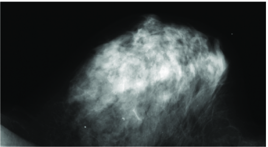
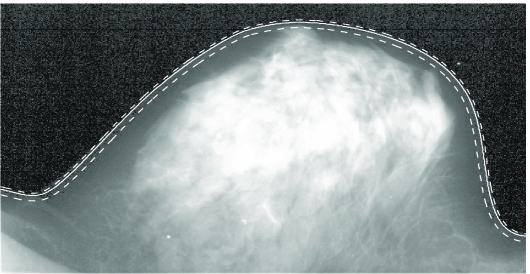
Figure 10 (left) shows a typical digitized mammogram image, characterised by a low contrast-to-noise ratio. A probability integral transform improves the contrast by increasing the dynamic range of image intensities (Figure 10, centre). The solid white line in Figure 10 (centre and insets on right) shows the reconstructed boundary $\overline{\Gamma}_{n}.$ Note that what appears to be a nipple is, in fact, a duct system leading to the nipple, so that the estimators correctly follow the skin line.

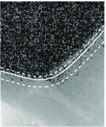
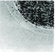
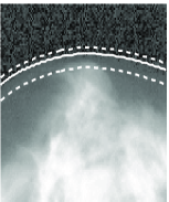
The 95% confidence set (dashed) for the true boundary in Figure 10 is obtained using a bootstrap resampling of size 1000. The confidence set is tight and fits the image well. It also shows that the reconstructed boundary is more variable toward the inside of the breast tissue. The background of the black and white mammogram image has considerably more noise than the foreground. Consequently, the posterior boundary samples show more variability toward the inside of the tissue. More details can be seen in insets in Figure 10 (right).

Note also that to apply our methods, we have assumed that the observed ODFs $b_{T_{i}}(x)$ are independent and identically distributed, whilst the boundary reconstruction is based on Markov chain Monte Carlo sampling from the posterior. To ensure the independence of the curve samples, we construct the confidence set for the boundary using 100 samples from the posterior, which were acquired every 250th sweep after a burn-in period of 1000 sweeps.

6 Discussion

In this paper, we studied consistency of set and boundary averages under random sampling. We also presented a method for the construction of confidence regions for the mean set and mean boundary. The confidence regions, though conservative, have appealing equivariance properties and are straightforward to implement. Simulations indicate that they achieve good coverage probabilities. Unlike previous developments, our methods are applicable to both convex and non-convex sets and allow for differences in local variability.

As there exists no notion of the standard deviation of a random set, one can also use the confidence regions as an informal assessment of the variability of the mean set estimator. This relationship is strengthened by the aforementioned equivariance properties, which mimic the scaling properties of the standard deviation and confidence region in the univariate setting.

In Section 5 we considered several empirical examples. The observed sets in these cases are non-convex, and therefore methods based on the Aumann expectation would not work well, although they may yield reasonable approximations for the sand grains example. In Section 5.5 we applied the proposed methods to a boundary reconstruction problem in a mammogram image. There, the confidence region technique was used to assess the variability of the MCMC estimation of the posterior mean. The proposed method was able to detect an increase in the variability of the sampling toward the inside of the breast tissue. A dilation method, such as one based on the results of Molchanov (1998), would not be able to detect this difference.

Appendix

Recall that the boundary of a set $A\subset\mathbb{R}^{d}$ is $C_{k}$ in a neighbourhood $N(x_{0})$ if there exists a bijective map $m:N(x_{0})\mapsto B_{1}(0)$, which is $C^{k}$ and whose inverse is also $C^{k}$, which maps the boundary into the set $\{x\in B_{1}(0):x_{d}=0\}.$ That is, the boundary is $C^{k}$ at $x_{0}$ if locally it is a $C^{k}$ manifold.

Proof of Proposition 2.3.

We first note that the condition $|\nabla E[b_{\bm{A}}(x_{0})]|\neq 0$ is necessary. For example, if $E[b_{\bm{A}}(x)]$ has a local minimum at $x_{0}$ then the boundary of $E[\bm{A}]$ contains the isolated point $\{x_{0}\}$, and no smoothness properties may be carried from the expected oriented distance function to the expected boundary.

Write $x=(x_{1},\ldots,x_{d})\in\mathbb{R}^{d}$ with $x_{0}=(x_{0,1},\ldots,x_{0,d}).$ Since $|\nabla E[b_{\bm{A}}(x_{0})]|\neq 0$, there exists a $j$ such that $\partial_{j}E[b_{\bm{A}}(x_{0})]\neq 0.$ Let $x_{(j)}=(x_{1},\ldots,x_{j-1},x_{j+1},\ldots,x_{d})\in\mathbb{R}^{d-1},$ and define $H:\mathbb{R}^{d-1}\times\mathbb{R}\mapsto\mathbb{R}$ by $H(x_{(j)},x_{j})=E[b_{\bm{A}}(x)].$ The boundary is now described via the set $H(x_{(j)},x_{j})=0$ and we may apply the implicit function theorem (Theorem 1-12, page 41 of Spivak (1965) and Theorem 31 p. 299 of Schwartz (1981)). The differentiability condition on the Jacobian in the implicit function theorem holds since

$$\partial_{x_{j}}H(x_{(j)},x_{j})=\partial_{j}E[b_{\bm{A}}(x_{0})]\neq 0.$$

It follows that there exists a function $g(x_{(j)})$, a neighbourhood of $(x_{1,0},\ldots,x_{j-1,0},x_{j+1,0},\ldots,x_{d})$, $N_{1}\subset\mathbb{R}^{d-1}$, and a neighbourhood of $x_{j,0}$, $N_{2}\subset\mathbb{R}$ such that $g:N_{1}\mapsto N_{2}$ is $C^{k}$ and describes the boundary, $\Gamma[\bm{A}]$, near $x_{0}$. ∎

Proof of Theorem 2.5.

Pointwise convergence follows immediately by the law of large numbers. Since both $\bar{b}_{n}(x)$ and $E[b_{\bm{A}}(x)]$ are Lipschitz functions (Jankowski and Stanberry, 2010), we also obtain uniform convergence over compact sets. ∎

The next result may be found, for example, in Kunita (1990, Theorem 1.4.7). We repeat it here for convenience.

Theorem 6.1 (Kolmogorov’s tightness criterion.).

For a compact set $\mathcal{D}\subset\mathbb{R}^{d}$, let $\{Y_{n}(x):x\in\mathcal{D}\}$ be a sequence of continuous random fields with values in $\mathbb{R}$. Assume that there exist positive constants $\gamma,C$ and $\alpha_{1},\ldots,\alpha_{d}$ with $\sum_{i=1}^{d}\alpha_{i}^{-1}<1$ such that

$$E[|Y_{n}(x)-Y_{n}(y)|^{\gamma}] \leq C\left(\sum_{i=1}^{d}|x_{i}-y_{i}|^{\alpha_{i}}\right)\ \ \mbox{ for all }x,y\in\mathcal{D},$$

$$E[|Y_{n}(x)|^{\gamma}] \leq C,\ \ \ \mbox{ for all }x\in\mathcal{D},$$

holds for any $n$. Then $\{Y_{n}\}$ is tight in $C(\mathcal{D})$.

Lemma 6.2.

There exists a constant $C(d)$, depending only on $d$, such that

$$E\left[|\mathbb{Z}_{n}(x)-\mathbb{Z}_{n}(y)|^{2d}\right] \leq C(d)|x-y|^{2d},$$

for any $n$ and $x,y\in\mathcal{D}.$

Proof.

The case $d=1$ is immediate. Next, consider $d=2$,

$$E\left[|\mathbb{Z}_{n}(x)-\mathbb{Z}_{n}(y)|^{4}\right] = n^{-2}\sum_{i,j,k,l=1}^{n}E\left[b^{*}_{i}b^{*}_{j}b^{*}_{k}b^{*}_{l}\right],$$

where $b^{*}_{i}=b_{i}(x)-b_{i}(y)-E[b_{\bm{A}}(x)]+E[b_{\bm{A}}(y)],$ and $|b^{*}_{i}|\leq 2|x-y|$ almost surely, since both $b_{i}$ and $E[b_{\bm{A}}]$ are Lipschitz (cf. Jankowski and Stanberry (2010)). Since the sampling is IID, and the $b^{*}_{i}$ are centred, it follows that the right-hand side of the above display is equal to

$$n^{-2}\left\{nE[(b_{1}^{*})^{4}]+3n(n-1)E[(b_{1}^{*})^{2}]^{2}\right\}\leq 64|x-y|^{4}.$$

Similarly, for $d=3,$

$$E\left[|\mathbb{Z}_{n}(x)-\mathbb{Z}_{n}(y)|^{6}\right]$$

$$= n^{-3}\sum_{i,j,k,l,p,t=1}^{n}E\left[b^{*}_{i}b^{*}_{j}b^{*}_{k}b^{*}_{l}b^{*}_{p}b^{*}_{t}\right]$$

$$= n^{-3}\left\{nE[(b_{1}^{*})^{6}]\right.$$

$$\hskip 28.45274pt+3n(n-1)\left(E[(b_{1}^{*})^{3}]^{2}+E[(b_{1}^{*})^{2}]E[(b_{1}^{*})^{4}]\right)$$

$$\left.\ \ \ \ \ \hskip 28.45274pt+\ 90n(n-1)(n-2)E[(b_{1}^{*})^{2}]^{3}\right\}$$

$$\leq 97\cdot 2^{6}\cdot|x-y|^{6}.$$

In general, the expansion becomes

$$n^{-d}\left\{nE[(b_{1}^{*})^{2d}]+\ldots\right.$$

$$\left.\hskip 14.22636pt+{2d\choose 2\ 2\ \ldots\ 2}n(n-1)\ldots(n-d+1)E[(b_{1}^{*})^{2}]^{d}\right\},$$

which is bounded above by $C(d)|x-y|^{2d}$, for some constant $C(d).$ ∎

Proof of Theorem 2.6.

Recall that $b_{\bm{A}}(x)$ is almost surely Lipschitz. Then $E[b_{\bm{A}}(x_{0})^{2}]<\infty$ for some $x_{0}\in\mathcal{D},$ implies that $E[b_{\bm{A}}(x)^{2}]<\infty$ for all $x\in\mathcal{D}$. Therefore, convergence in finite dimensional distributions is immediate by the multidimensional central limit theorem, and it remains to prove that the process $\mathbb{Z}_{n}$ is tight in the space of continuous functions on $\mathcal{D}$. However, this is straightforward if we use Theorem 6.1.

The first condition with $\gamma=2d$ and $\alpha_{i}=2d$ for all $i$, follows immediately from Lemma 6.2 by Jensen’s inequality. For the second condition we need to bound $E[\mathbb{Z}_{n}(x)^{2d}]$ uniformly. This follows easily since, for some fixed $x_{0}\in\mathcal{D}$,

$$E\left[\mathbb{Z}_{n}(x)^{2d}\right]\leq C^{\prime}\left(E\left[\mathbb{Z}_{n}(x_{0})^{2d}\right]+E\left[|\mathbb{Z}_{n}(x)-\mathbb{Z}_{n}(y)|^{2d}\right]\right)$$

for come constant $C^{\prime}$ (depending on $d$), again applying Jensen’s inequality. We have already placed a bound on the second term of the right-hand side of the above equation, and a bound on the first term follows from the central limit theorem. ∎

Let $\mathcal{D}$ be a compact subset of $\mathbb{R}^{d}.$ We recall a theorem of Winkler (1964). Proposition 2.7 follows immediately.

Theorem 6.3 (SATZ 6 on page 837 of Winkler (1964)).

Let $\{Y(x),x\in\mathcal{D}\subset\mathbb{R}^{d}\}$ be a Gaussian random field such that for $\tau\rightarrow 0$ the inequality

$$E\left[\left|Y(x+\tau)-Y(x)\right|^{2}\right]\leq C|\tau|^{\varepsilon}$$

holds for some $\varepsilon>0$ and $0<C<\infty$. Then for almost all realizations there exists a random number $\delta(\omega)$ so that for any $x_{1},x_{2}\in\mathcal{D}$ with $|x_{1}-x_{2}|<\delta(\omega)$ and $0<\eta<\varepsilon/2$ the inequality

$$|Y(x_{1})-Y(x_{2})|\leq C_{0}|x_{1}-x_{2}|^{\eta}$$

holds. In particular, it follows that $\{Y(x),x\in\mathcal{D}\}$ is continuous with probability one.

Proof of Proposition 2.7.

To prove this result we again recall that both $|b_{\bm{A}}(x)-b_{\bm{A}}(y)|\leq|x-y|$ almost surely. Therefore,

$$\mbox{var}(\mathbb{Z}(x)-\mathbb{Z}(y)) = \mbox{var}(b_{\bm{A}}(x)-b_{\bm{A}}(y))$$

$$\leq E[(b_{\bm{A}}(x)-b_{\bm{A}}(y))^{2}]\leq|x-y|^{2}.$$

A similar approach shows the bound for the covariance. We may now use this result, along with Theorem 6.3 to prove that the sample paths of $\mathbb{Z}$ are continuous almost surely. ∎

Proof of Theorem 3.1.

The first part of the theorem follows directly from Molchanov (1998, Theorem 2.1). The second part follows from Cuevas et al. (2006, Theorem 1), but some further explanations are necessary. Without loss of generality, we may assume that $\mathcal{D}$ is compact. Therefore, note that (M1) and (f2) of Cuevas et al. (2006, Theorem 1, page 9) are satisfied, and that the remaining condition (f1) holds under (3.1) and (3.2). Fix $\varepsilon>0$. To prove their result, they show that there exists an $n_{0}$ such that for all $n\geq n_{0}$

$$\partial\{x:E[b_{\bm{A}}(x)]\geq 0\} = \{x:E[b_{\bm{A}}(x)]=0\}$$

$$\subset \left(\partial\{x:\bar{b}_{n}\geq 0\}\right)^{\varepsilon}$$

$$\subset \{x:\bar{b}_{n}=0\}^{\varepsilon},$$

since $\bar{b}_{n}$ is continuous. We use the notation $A^{\varepsilon}=\cup_{x\in A}B_{\varepsilon}(x)$ here. Thus it remains to prove that for sufficiently large $n$,

$$\{x:\bar{b}_{n}=0\} \subset \{x:E[b_{\bm{A}}(x)]=0\}^{\varepsilon}.$$

This follows almost exactly as in Cuevas et al. (2006, Theorem 1).

By contradiction, suppose that there exists a sequence $x_{n}\in\{x:\bar{b}_{n}=0\}$ such that $d(\{x_{n}\},\{x:E[b_{\bm{A}}(x)]=0\})>~{}\varepsilon$ for all $n$. By compactness, there exists an $x_{0}$ such that $x_{n}\rightarrow x_{0}$, and by continuity, we have that $E[b_{\bm{A}}(x_{0})]=0$, almost surely. Therefore, $d(\{x_{n}\},\{x:E[b_{\bm{A}}(x)]=0\})\leq|x_{n}-x_{0}|\rightarrow 0,$ which is a contradiction. ∎

Proof of Proposition 3.3.

The statements are immediate from definitions and continuity of $E[b_{\bm{A}}(x)]$. ∎

Proof of Proposition 4.2.

Let $\bar{b}_{n}$ denote the average ODF for the observed sets $A_{i},$ and $\bar{b}_{n}^{1}$ denote the average ODF for the observed sets $\alpha A_{i}.$ For any $\alpha>0$, we have $b_{\alpha A}(x)=\alpha b_{A}(x/\alpha)$. It follows that $\bar{b}_{n}^{1}(x)=\alpha\bar{b}_{n}(x/\alpha)$ and $E[b_{\bm{A}_{1}}(x)]=\alpha E[b_{\bm{A}}(x/\alpha)]$. Next,

$$\mathbb{Z}_{n}^{1}(x) = \sqrt{n}(\bar{b}_{n}^{1}(x)-E[b_{\bm{A}_{1}}(x)])$$

$$= \alpha\sqrt{n}(\bar{b}_{n}-E[b_{\bm{A}}])(x/\alpha).$$

Therefore, $\mathbb{Z}_{n}^{1}(x)\Rightarrow\mathbb{Z}^{1}(x)\stackrel{{\scriptstyle d}}{{=}}\alpha\mathbb{Z}(x/\alpha).$ Lastly, note that

$$\sup_{x\in\mathcal{W}_{1}}\mathbb{Z}^{1}(x)\stackrel{{\scriptstyle d}}{{=}}\sup_{x\in\alpha\mathcal{W}}\alpha\mathbb{Z}(x/\alpha)=\alpha\sup_{x\in\mathcal{W}}\mathbb{Z}(x).$$

Therefore, a confidence region for $E[\bm{A}_{1}]\cap\mathcal{W}_{1}$ is

$$\{x\in\mathcal{W}_{1}:\bar{b}_{n}^{1}(x)\leq\alpha q_{1}/\sqrt{n}\}$$

$$= \{x\in\alpha\mathcal{W}:\alpha\bar{b}_{n}(x/\alpha)\leq\alpha q_{1}/\sqrt{n}\}$$

$$= \{x\in\alpha\mathcal{W}:\bar{b}_{n}(x/\alpha)\leq q_{1}/\sqrt{n}\}$$

$$= \alpha\{x\in\mathcal{W}:\bar{b}_{n}(x)\leq q_{1}/\sqrt{n}\},$$

and similarly for $\Gamma[\bm{A}_{1}]\cap\mathcal{W}_{1}.$

The same argument works for a rigid motion $g$, since $b_{g(A)}(x)=b_{A}(g^{-1}(x))$. ∎

References

- Ayala et al. (1991) Ayala, G., Ferrandiz, J. and Montes, F. (1991). Random set and coverage measure. Adv. Appl. Prob. 23 972–974.
- Baddeley and Molchanov (1998) Baddeley, A. and Molchanov, I. (1998). Averaging of random sets based on their distance functions. J. Math. Imaging Vision 8 79–92.
- Bookstein et al. (2002a) Bookstein, F. L., Sampson, P. D., Connor, P. D. and Streissguth, A. P. (2002a). Midline corpus callosum is a neuroanatomical focus of fetal alcohol damage. The Anatomical record 269 162–174.
- Bookstein et al. (2002b) Bookstein, F. L., Streissguth, A. P., Sampson, P. D., Connor, P. D. and Barr, H. M. (2002b). Corpus callosum shape and neuropsychological deficits in adult males with heavy fetal alcohol exposure. NeuroImage 15 233–251.
- Breu et al. (1995) Breu, H., Gil, J., Kirkpatrick, D. and Werman, M. (1995). Linear time euclidean distance transform algorithms. IEEE Trans. Pattern Anal. Mach. Intell. 17 529–533.
- Cuevas et al. (2006) Cuevas, A., González-Manteiga, W. and Rodríguez-Casal, A. (2006). Plug-in estimation of general level sets. Aust. N. Z. J. Stat. 48 7–19.
- Delfour and Zolésio (1994) Delfour, M. C. and Zolésio, J.-P. (1994). Shape analysis via oriented distance functions. J. Funct. Anal. 123 129–201.
- Delfour and Zolésio (2001) Delfour, M. C. and Zolésio, J.-P. (2001). Shapes and geometries, vol. 4 of Advances in Design and Control. Society for Industrial and Applied Mathematics (SIAM), Philadelphia, PA. Analysis, differential calculus, and optimization.
- Ding et al. (2008) Ding, J., Warren, R., Warsi, I., Day, N., Thompson, D., Brady, M., Tromans, C., Highnam, R. and Easton, D. (2008). Evaluating the effectiveness of using standard mammogram form to predict breast cancer risk: Case-control study. Cancer Epidemiology Biomarkers and Prevention 17 1074–1081.
- Freidman et al. (1977) Freidman, J., Bentley, J. and Finkel, R. (1977). An algorithm for finding best matches in logrithmic expected time. ACM Trans. Pattern Anal. Softw. 3 209–226.
- Friel and Molchanov (1999) Friel, N. and Molchanov, I. (1999). A new thresholding technique based on random sets. Pattern Recognition 32 1507–1517.
- Jankowski and Stanberry (2010) Jankowski, H. and Stanberry, L. (2010). Expectations of random sets and their boundaries using oriented distance functions. J. Math. Imaging Vision 36 291–303.
- Kent et al. (2000) Kent, J. T., Dryden, I. L. and Anderson, C. R. (2000). Using circulant symmetry to model featureless objects. Biometrika 87 527–544.
- Kunita (1990) Kunita, H. (1990). Stochastic flows and stochastic differential equations, vol. 24 of Cambridge Studies in Advanced Mathematics. Cambridge University Press, Cambridge.
- Levitt et al. (2009) Levitt, J., Styner, M., M., N., S., B., Koo, M., Voglmaier, M., Dickey, C., Niznikiewicz, M., Kikinis, R., McCarley, R. and Shenton, M. (2009). Shape abnormalities of caudate nucleus in schizotypal personality disorder. Schizophr Res 110 127–139.
- Lewis et al. (1999) Lewis, T., Owens, R. and Baddeley, A. (1999). Averaging feature maps. Pattern Recognition 32 1615–1630.
- Matheron (1975) Matheron, G. (1975). Random sets and integral geometry. John Wiley & Sons, New York-London-Sydney. With a foreword by Geoffrey S. Watson, Wiley Series in Probability and Mathematical Statistics.
- Molchanov (2005) Molchanov, I. (2005). Theory of random sets. Probability and its Applications (New York), Springer-Verlag London Ltd., London.
- Molchanov and Terán (2003) Molchanov, I. and Terán, P. (2003). Distance transforms for real-valued functions. J.Math.Anal.Appl. 278 472–484.
- Molchanov (1998) Molchanov, I. S. (1998). A limit theorem for solutions of inequalities. Scandinavian Journal of Statistics 25 235–242.
-
R Development Core Team (2009)
R Development Core Team (2009).
R: A Language and Environment for Statistical Computing.
R Foundation for Statistical Computing, Vienna, Austria.
ISBN 3-900051-07-0.
URL http://www.R-project.org - Rosenfeld and Pfaltz (1966) Rosenfeld, A. and Pfaltz, J. (1966). Sequential operations in digital picture processing. J. ACM 13 471–494.
- Schwartz (1981) Schwartz, L. (1981). Cours d’analyse. 1. 2nd ed. Hermann, Paris.
- Scutt et al. (1997) Scutt, D., Manning, J., Whitehouse, G., Leinster, S. and Massey, C. (1997). The relationship between breast asymmetry, breast size and the occurrence of breast cancer. Br. J. Radiol 70 1017–1021.
- Seri and Choirat (2004) Seri, R. and Choirat, C. (2004). Confidence sets for the Aumann mean of a random closed set. In Lecture Notes in Computer Science, vol. 3045, Proceedings of ICCSA 2004, International Conference in Computational Science and its Applications. 298–307.
- Serra (1984) Serra, J. (1984). Image analysis and mathematical morphology. Academic Press Inc. [Harcourt Brace Jovanovich Publishers], London. English version revised by Noel Cressie.
- Spivak (1965) Spivak, M. (1965). Calculus on manifolds. A modern approach to classical theorems of advanced calculus. W. A. Benjamin, Inc., New York-Amsterdam.
- Stanberry and Besag (2009) Stanberry, L. and Besag, J. (2009). Boundary reconstruction in binary images using splines. Preprint.
- Stoyan and Molchanov (1997) Stoyan, D. and Molchanov, I. S. (1997). Set-valued means of random particles. J. Math. Imaging Vision 7 111–121.
- Styner et al. (2003) Styner, M., Gerig, G., Lieberman, J., Jones, D. and Weinberger, D. (2003). Statistical shape analysis of neuroanatomical structures based on medial models. Medical Image Analysis 7 207 – 220. Functional Imaging and Modeling of the Heart.
- Styner et al. (2004) Styner, M., Lieberman, J. A., Pantazis, D. and Gerig, G. (2004). Boundary and medial shape analysis of the hippocampus in schizophrenia. Medical Image Analysis 8 197–203.
- Winkler (1964) Winkler, W. (1964). Stetigkeitseigenschaften der Realisierungen Gauss’scher zufälliger Felder. In Trans. Third Prague Conf. Information Theory, Statist. Decision Functions, Random Processes (Liblice, 1962). Publ. House Czech. Acad. Sci., Prague, 831–839.
Appendix
Recall that the boundary of a set is in a neighbourhood if there exists a bijective map , which is and whose inverse is also , which maps the boundary into the set That is, the boundary is at if locally it is a manifold.