Selective excitations of transverse vibrational modes of a carbon nanotube through a “shuttle-like” electromechanical instability

Abstract

We study the dynamics of transverse oscillations of a suspended carbon nanotube into which current is injected from the tip of a scanning tunneling microscope (STM). In this case the correlations between the displacement of the nanotube and its charge state, determined by the position-dependent electron tunneling rate, can lead to a “shuttle-like” instability for the transverse vibrational modes. We find that selective excitation of a specific mode can be achieved by an accurate positioning of the STM tip. This result suggests a feasible way to control the dynamics of this nano-electromechanical system (NEMS) based on the “shuttle instability”.

There are several reasons for the considerable current interest in nano-electromechanical systems (NEMS), both for technological applications and fundamental research. The peculiar combination of several features such as high vibrational frequencies and small masses which characterize most NEMS makes these systems very suitable for the realization of new measurement tools with extremely high sensitivity in mass sensing and force microscopy applications [Roukes, 2000; Blencowe, 2005]. Furthermore, the mechanical elements of the NEMS (typically cantilevers or beams) are considered the most promising structures where quantum features of motion could be experimentally detected [Schwab and Roukes, 2005].

The physical basis for many of the interesting functionalities of NEMS is the strong interplay between mechanical and electronic degrees of freedom [Poncharal et al., 1999; Purcell et al., 2002; Sapmaz et al., 2003; Sazonova et al., 2004]. In the particular case of a nano-electromechanical single-electron transistor device having a metallic dot as movable part, the equilibrium position of the dot can become unstable as a consequence of the electromechanical coupling. In this case the dominant mechanism for the transport of charge is based on the oscillations of the dot which can “shuttle” the tunneling electrons across the system [Gorelik et al., 1998; Moskalenko et al., 2009].

The typical set-up for many NEMS includes a spatially extended movable element such as a suspended carbon nanotube, whose dynamics has been demonstrated to be characterized by a number of different vibrational modes [Hüttel et al., 2008]. The relevance of many mechanical modes in the transport of charge suggests that the variety of effects due to the electromechanical coupling in suspended carbon nanotube-based NEMS may be even richer than in the ordinary “shuttle” system. Jonsson et al. have shown [Jonsson et al., 2005, 2007, 2008] that if extra charge is injected into the movable part of the device from the tip of a scanning tunneling microscope (STM) a nano-electromechanical “shuttle-like” instability can be induced for the transverse vibrational modes of the nanotube.

The selective promotion of the electromechanical instability for different vibrational modes provides an interesting perspective for probing the dynamics of NEMS. Here we show that such selective excitation can be achieved by means of local injection of electric charge. The main idea is to optimize the electromechanical coupling for the mode(s) which we want to make unstable. The local character of the electric charge injection makes the selective excitation of the nanotube transverse modes possible by varying the position of the STM tip.

We will consider here the same device analyzed by Jonsson et al. since it provides a convenient set-up to control the electromechanical coupling of different vibrational modes. The system is sketched in Fig. (1) and it consists of a suspended metallic carbon nanotube in tunneling contact with an STM tip and one supporting lead.

We take the $z$-axis along the nanotube axis, while its cross section lies in the $xy$ plane. The STM tip is put over point (0, 0, $z_{0}$) and its distance from the nanotube at equilibrium is $d\simeq$1 nm.

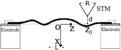
Figure 1: Sketch of the model system considered. The distance of the suspended carbon nanotube from the STM tip affects the electron tunneling rate between them, while the tunneling rate between the nanotube and the leads is constant (the vibration amplitude and the STM-nanotube equilibrium distance $d$ shown are exaggerated for clarity).

In order to describe the motion of the nanotube we model it as a classical elastic beam of length $L$ clamped at both ends and focus on its flexural vibrations.

The motion of the nanotube in the $xz$ plane can be described through $u(z,t)$, its displacement along the $x$ axis from the static equilibrium configuration. If the amplitude of the oscillations is small enough for linear elasticity theory to be valid, the time evolution of $u(z,t)$ is determined by the following equation [Cleland, 2003]:

$$\rho S\frac{\partial^{2}u}{\partial t^{2}}+\frac{EI}{L^{4}}\frac{\partial^{4}u}{\partial z^{4}}=F_{x}^{\rm el}(N(t),z,z_{0}).$$ (1)

In Eq. (1), $\rho$ is the carbon nanotube density, $S$ the cross section, $E$ the Young modulus, $I$ the cross section moment of inertia, $N(t)$ the number of extra electrons on the nanotube at time $t$ and $F_{x}^{\rm el}$ the $x$ component of the external force (per unit length) generated by the electrostatic interaction between the STM tip and the nanotube.

The precise spatial distribution of $F_{x}^{\rm el}$ depends on the details of the geometric structure of the tip apex. However, a simple electrostatic analysis indicates that for $|z-z_{0}|\gg R$, $d$ (where $R\lesssim 10^{-8}$ m is the effective size of the STM tip), the force $F_{x}^{\rm el}$ decays at least as $|z-z_{0}|^{-3}$. Therefore the influence of the metallic leads can be ignored as long as the STM tip is not too close to them and we can write $F_{x}^{\rm el}(N,z,z_{0})\simeq F_{x}^{\rm el}(N,z-z_{0})$.

The displacement field $u(z,t)$ and the force per unit length $F_{x}^{\rm el}$ can be expressed as linear combinations of eigenfunctions $\varphi_{j}(z)$ of the operator $d^{4}/dz^{4}$ with the boundary conditions $u(0,t)=u(L,t)=0$, $du/dz(0,t)=du/dz(L,t)=0$.

The expansion of $u(z,t)$ and $F_{x}^{\rm el}$ over the complete set of functions $\varphi_{j}(z)$ makes it possible to decompose Eq. (1) into a set of equations of motion for the eigenmode amplitudes $x_{j}(t)$, which can be written in hamiltonian form by introducing the conjugate momenta $\pi_{j}(t)$:

$$\dot{x}_{j} =\frac{\pi_{j}}{m}$$ (2a)

$$\dot{\pi}_{j} +\gamma_{j}\pi_{j}+m\omega_{j}^{2}x_{j}=Lf_{j}^{\rm el}(N(t),\{x_{j}\},z_{0}).$$ (2b)

In Eqs. (2), $f_{j}^{\rm el}$ are the coefficients in the expansion of $F_{x}^{\rm el}$ over the complete set of functions $\varphi_{j}(z)$ (which are chosen to be dimensionless), $m=\rho SL$ is the mass of the nanotube and $\omega_{j}$ are the frequencies of the transverse vibrational modes, given by $\omega_{j}=\sqrt{k_{j}EI/(\rho SL^{2})}$, where the eigenvalues $k_{j}$ can be found by solving: $\textrm{cos}k_{j}^{1/4}\textrm{cosh}k_{j}^{1/4}=1$.

We introduced in Eq. (2b) a phenomenological damping force for each mode, $-\gamma_{j}\pi_{j}$, where $\gamma_{j}$ has the dimension of inverse time. The motion of the nanotube is inevitably affected by dissipative mechanisms, which can be related to its coupling to the environment and to several internal processes. We will later consider a general form for $\gamma_{j}$ which can be used to describe the damping induced by a wide class of phenomena.

An approximate expression for the force coefficients $f_{j}^{\rm el}$ in Eq. (2b) can be found through some physical considerations on the characteristic lengths of the system. Since the eigenfunctions $\varphi_{j}(z)$ vary appreciably only over distances of the order of $L$, we can express each $f_{j}^{\rm el}$ as a sum of a sharply localized contribution at $z_{0}$ plus a correction:

$$Lf_{j}^{\rm el} =\int_{-L/2}^{L/2}F_{x}^{el}(N(t),z^{\prime}-z_{0})\varphi_{j}(z^{\prime})dz^{\prime}=$$

$$=eN(t)\mathcal{E}\varphi_{j}(z_{0})+O\left(R^{2}/L^{2}\right),$$ (3)

where $\mathcal{E}$ is a phenomenological parameter which provides the magnitude of the effective electrostatic field between the STM and the nanotube.

The size of the correction in Eq. (Selective excitations of transverse vibrational modes of a carbon nanotube through a “shuttle-like” electromechanical instability) can be estimated in terms of the characteristic lengths of the system: for the typical values $L\sim 10^{-7}$ m and $R\sim 10^{-8}$ m, the condition $R^{2}/L^{2}\ll 1$ is fulfilled and that defines the range of validity of the approximation $Lf_{j}^{\rm el}\simeq eN(t)\mathcal{E}\varphi_{j}(z_{0})$ which we will use from now on.

For what concerns the transport of charge the system is equivalent to a double tunnel junction, having one potential barrier localized between the STM tip and the nanotube and the another one between the nanotube and the leads. In our analysis we will consider the case of electrons for which the inverse characteristic time of decoherence is much shorter than the tunneling rates, so that the description of tunneling as a stochastic (rather than coherent) process is sufficient.

Following the approach presented in [Armour et al., 2004] for a point-like oscillator coupled to a single-electron transistor, we define a probability density in the phase space of the system $P_{N}(\vec{x},\vec{\pi},t)$ such that $P_{N}(\vec{x},\vec{\pi},t)dx_{1}d\pi_{1}dx_{2}d\pi_{2}\ldots$ (with all the $x_{j}$ and $\pi_{j}$ scaled by proper dimensional factors) is the joint probability that at time $t$ there are $N$ electrons in excess on the nanotube while the eigenmode amplitudes and momenta $\{x_{j}\}$, $\{\pi_{j}\}$ take values in the phase space region defined by $\prod_{j}dx_{j}d\pi_{j}\equiv d\vec{x}d\vec{\pi}$.

We consider the system in the Coulomb blockade regime and limit to one the maximum number of extra electrons on the nanotube, therefore only the probability densities $P_{0}(\vec{x},\vec{\pi},t)$ and $P_{1}(\vec{x},\vec{\pi},t)$ play a role in the description of the nanotube dynamics.

The coupling between the mechanical and electronic degrees of freedom arises because the tunneling rate between the STM tip and the nanotube, $\Gamma_{\rm STM-NT}(\vec{x},z_{0})$ is affected by their relative distance at point $z_{0}$: $\Gamma_{\rm STM-CNT}(\vec{x},z_{0})=\Gamma_{0}\exp((-d+\sum_{j}x_{j}\varphi_{j}(z_{0}))/\lambda)$, where $\lambda$ is the effective tunneling length of the STM-nanotube junction and $\Gamma_{0}$ is a constant. The factor $\Gamma_{0}^{*}(d)\equiv\Gamma_{0}\exp{(-d/\lambda)}$ is the tunneling rate that would characterize the junction if the motion of the nanotube could be neglected. The tunneling rate between the nanotube and the leads, $\Gamma_{\rm NT-L}$ does not depend on the nanotube displacement.

We remark that all the tunneling rates are generally functions of the bias voltage. However, since here we always assume $V$ fixed at some value we never explicitly indicate the dependence on $V$. In order to be consistent with the condition of single-electron charging of the nanotube, the electron temperature and the bias voltage have to be in the range: $k_{\rm B}T<E_{\rm C}<eV<2E_{\rm C}$, where $E_{\rm C}$ is the energy required to add one extra electron to the nanotube.

The time evolution of the probability densities $P_{+}(\vec{x},\vec{\pi},t)\equiv P_{1}(\vec{x},\vec{\pi},t)+P_{0}(\vec{x},\vec{\pi},t)$ and $P_{-}(\vec{x},\vec{\pi},t)\equiv P_{1}(\vec{x},\vec{\pi},t)-P_{0}(\vec{x},\vec{\pi},t)$ is determined by the equations:

$$\frac{\partial P_{+}}{\partial t}+(\mathcal{L}_{1} +\mathcal{L}_{2})(P_{+}+P_{-})=0$$ (4a)

$$\frac{\partial P_{-}}{\partial t}+(\mathcal{L}_{1} +\mathcal{L}_{2})(P_{+}+P_{-})=$$

$$=\Gamma_{-}(\vec{x};z_{0})P_{+}+\Gamma_{+}(\vec{x};z_{0})P_{-},$$ (4b)

where $\Gamma_{+}(\vec{x};z_{0})\equiv\Gamma_{\rm STM-NT}(\vec{x};z_{0})+\Gamma_{\rm NT-L}$, $\Gamma_{-}(\vec{x};z_{0})\equiv\Gamma_{\rm STM-NT}(\vec{x};z_{0})-\Gamma_{\rm NT-L}$ and the Liouvillian operators $\mathcal{L}_{1}$ and $\mathcal{L}_{2}$ are defined as follows:

$$\mathcal{L}_{1} \equiv\sum_{j}\left[\frac{\pi_{j}}{m}\frac{\partial}{\partial x_{j}}-m\omega_{j}^{2}x_{j}\frac{\partial}{\partial\pi_{j}}+\gamma_{j}\frac{\partial}{\partial\pi_{j}}\pi_{j}\right]$$

$$\mathcal{L}_{2} \equiv e\mathcal{E}\sum_{j}\varphi_{j}(z_{0})\frac{\partial}{\partial\pi_{j}}.$$

From Eqs. (4) we can derive the equations of motion for any dynamical variable averaged over the probability densities $P_{+}$ and $P_{-}$: $\langle(\ldots)\rangle_{\alpha}\equiv\int(\ldots)P_{\alpha}(\vec{x},\vec{\pi},t)d\vec{x}d\vec{\pi}$, where $\alpha=\pm$. The set of equations of motion for the first moments $\langle 1\rangle_{-}\equiv p_{-}(t)$, $\langle x_{j}\rangle_{\alpha}$, $\langle\pi_{j}\rangle_{\alpha}$ is:

$$\frac{d\langle x_{j}\rangle_{\alpha}}{dt} =\frac{\langle\pi_{j}\rangle_{\alpha}}{m}$$ (5a)

$$\frac{d\langle\pi_{j}\rangle_{\alpha}}{dt} =-m\omega_{j}^{2}\langle x_{j}\rangle_{\alpha}-\gamma_{j}\langle\pi_{j}\rangle_{\alpha}+e\mathcal{E}\varphi_{j}(z_{0})p_{1}$$ (5b)

$$\frac{dp_{-}}{dt} =\langle\Gamma_{-}(\vec{x};z_{0})\rangle_{+}-\langle\Gamma_{+}(\vec{x};z_{0})\rangle_{-},$$ (5c)

The set of equations (5) is not closed because the exponential form of the tunneling rate $\Gamma_{\rm STM-NT}(\vec{x};z_{0})$ introduces a coupling between the first and all the other moments. However in the limit of small oscillation amplitudes we can expand $\Gamma_{\rm STM-NT}(\vec{x};z_{0})$ to first order in $x_{j}/\lambda$ and that reduces (5) to a closed set of linear equations.

The static solution of the linearized equations of motion, $\langle\pi_{j}\rangle_{\alpha}=0$, $\langle x_{j}^{\alpha}\rangle_{\alpha}=\bar{x}_{j}^{\alpha}$, $p_{-}=\bar{p}$, where $\bar{x}_{j}^{\alpha}$ and $\bar{p}$ are constant, describes the nanotube as a slightly bent beam at rest. The stability of this solution can be investigated by substituting the expressions $\langle\xi_{k}\rangle_{+}\equiv\bar{\xi}_{k}+A_{k}e^{\beta_{k}t}$ (where $\xi_{k}$ is any of the dynamical variables $\langle x_{k}\rangle$, $\langle\pi_{k}\rangle$, $p_{-}$ and $A_{k}$ is constant) in the linearized equations of motion and solving for the exponents $\beta_{k}$ [Strogatz, 2001].

This procedure leads to an algebraic equation which in general cannot be solved analytically. However, if the dimensionless parameters $\varepsilon_{k}\equiv e\mathcal{E}\varphi^{2}_{k}(z_{0})/(m\omega_{k}^{2}\lambda)$ are much smaller than 1 and the nanotube is only weakly damped ($\gamma_{k}\ll\omega_{k}$), we can look for exponents of the form $\beta_{k}\sim i\omega_{k}+\delta_{k}$, with $|\delta_{k}|\ll\omega_{k}$ and derive an analytical expression for the $\delta_{k}$ which up to the first order in all $\varepsilon_{k}$ and $\gamma_{k}$ reads:

$$\delta_{k}=-\frac{\gamma_{k}}{2}+\frac{\Gamma_{0}^{*}(d)\Gamma_{\rm NT-L}}{2\Gamma_{+}^{*}(d)}\frac{\omega_{k}^{2}\varepsilon_{k}(z_{0})}{\omega_{k}^{2}+\Gamma_{+}^{*2}(d)}\left(1+i\frac{\Gamma_{+}^{*}(d)}{2\omega_{k}}\right),$$ (6)

where $\Gamma_{+}^{*}(d)\equiv\Gamma_{0}^{*}(d)+\Gamma_{\rm NT-L}$. The condition $\varepsilon_{k}\ll 1$ can be taken as a definition of the weak electromechanical regime, since it implies that the shift in the equilibrium position of the nanotube at point $z_{0}$ when it is charged by one extra electron, $\delta u\equiv e\mathcal{E}\sum_{j}\varphi_{j}^{2}(z_{0})/(m\omega_{j}^{2})$, is much smaller than the tunneling length $\lambda$. For realistic values of the parameters which are consistent with the conditions of validity of our model ($V\sim$ 0.1 V, the capacitances of the tunnel junctions $C_{\rm STM-NT}\sim C_{\rm NT-L}\sim 10^{-18}$ F as reported in [LeRoy et al., 2004], $\lambda\sim 10^{-10}$ m, $\omega_{k}\sim 10^{2}$ MHz), $m\sim 10^{-22}$ kg, $L\sim 10^{-7}$ m, the regime of weak electromechanical coupling is attained: $\varepsilon_{k}(z_{0})\lesssim 0.1$ for all the modes at every position $z_{0}$.

The sign of the real part of $\delta_{k}$ in Eq. (6) determines the stability of the static solution for the $k-$th average mode amplitude. If $\mathfrak{Re}[\delta_{k}]>0$ then $\langle x_{k}\rangle_{+}$ increases exponentially in time, hence the static solution for the $k$-th mode is unstable. This is the signature of a “shuttle-like” electromechanical instability. On the other hand, if $\mathfrak{Re}[\delta_{k}]<0$ the energy pumped into the vibrational mode by the electrostatic field is not able to compensate the loss due to dissipation and after a time interval of the order of $1/\gamma_{k}$ the $k$-th mode amplitude decays to its static value.

For fixed values of $\gamma_{k}$, $\mathcal{E}$ and $\Gamma_{2}$, the sign of $\mathfrak{Re}[\delta_{k}]$ becomes a function of $z_{0}$ and $\Gamma_{0}^{*}(d)$, i.e. it depends only on the position of the STM tip in the $xz$ plane. The set of values of $z_{0}$ and $\Gamma_{0}^{*}(d)$ for which the real part of $\delta_{k}$ is positive defines the instability region for the $k$-th mode amplitude in the plane ($z_{0}$,$\Gamma_{0}^{*}(d)$).

In order to map the instability regions we have to specify an analytic expression for the damping rates $\gamma_{k}$. The dissipation of mechanical energy in NEMS can take place through several mechanisms. However, in spite of the variety of the dissipative processes in solids, their effect on the NEMS performance can be described by considering the retardation induced in the NEMS response to mechanical perturbations (which adds to the “instantaneous” elastic behaviour).

In order to include this effect in our model we follow the approach introduced by Zener and formally replace the Young modulus with a frequency dependent complex function which results in the following expression for the damping rates: $\gamma_{k}\equiv Y\omega_{k}^{2}\tau/(1+\omega_{k}^{2}\tau^{2})$ [Cleland, 2003].

A large class of dissipative phenomena in solids (e.g. thermoelasticity, dislocations and defects dynamics) can be parametrized though the dimensionless coefficient $Y$ and the relaxation time $\tau$, which both depend on temperature as well as on several geometric and material properties [Nowick and Berry, 1972].

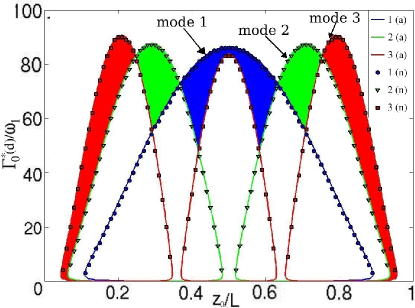
Figure 2: (Color online) Regions of instability in the parameter plane ($z_{0}$, $\Gamma_{0}^{*}(d)$) for the first three bending modes when the inverse characteristic time of the nanotube mechanical response to the external force is smaller than the frequencies of the nanotube vibrational modes, $1/\tau=0.1\omega_{1}$. The regions computed from the real part of the analytic expression (6) (solid lines) are compared with the results obtained by the numerical solution of the linearized equations of motion (markers). The parts of the plot filled with colors correspond to the values of ($z_{0}$, $\Gamma_{0}^{*}(d)$) for which a single vibrational mode is excited. The other relevant parameters are $e\mathcal{E}/(m\lambda\omega_{1}^{2})=0.1$, $\Gamma_{\rm NT-L}=5\omega_{1}$, $Y=10^{-4}$.

We first consider the limit in which the characteristic inverse time of the retarded mechanical response is much smaller than the frequencies of the nanotube eigenmodes: $1/\tau\ll\omega_{k}$. In this case the damping term in Eq. (6) does not depend on the frequency and the dissipation rate is the same for all the modes.

In Fig. (2) the instability regions determined by Eq. (6) for the first three modes are plotted together with the real parts of the exponents $\beta_{k}$ obtained from the numerical analysis of the linear stability problem. The areas filled with colours correspond to the values of ($z_{0}$, $\Gamma_{0}^{*}(d)$) for which only a single vibrational mode is unstable, while the regions where two or three modes are unstable are left blank.

The physical picture presented in Fig. (2) changes drastically in the opposite limit, $1/\tau\gg\omega_{k}$, as can be seen in Fig. (3). In this case the first mode is characterized by the smallest dissipation rate, $\gamma_{1}\ll\gamma_{k}\quad k\neq 1$, therefore if any of the modes is unstable, also the first one is unstable. That excludes the possibility of promoting a selective instability in the limit $1/\tau\gg\omega_{k}$.

The dynamical behaviour of the nanotube in the regime of single-mode instability is qualitatively the same of the ordinary “shuttle” system [Gorelik et al., 1998]. The amplitude of the oscillations increases exponentially until it reaches a certain steady value which depends on the parameters of the system. This transition is characterized by a large enhancement of the current (with respect to the static tunneling regime) that can be experimentally detected by measuring the current flowing through the device for different positions of the STM tip.

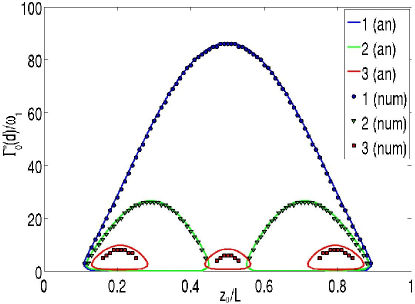
Figure 3: (Color online) Regions of instability in the parameter plane ($z_{0}$, $\Gamma_{0}^{*}(d)$) for the first three bending modes when the inverse characteristic time of the nanotube mechanical response to the external force is larger than the frequencies of the nanotube vibrational modes, $1/\tau=10\omega_{1}$. The regions computed from the real part of the analytic expression (6) (solid lines) are compared with the results obtained by the numerical solution of the linearized equations of motion (markers). The region of instability for the first mode includes all the values of ($z_{0}$, $\Gamma_{0}^{*}(d)$) for which the other modes are unstable, therefore no selective excitation can be attained in this regime. The other relevant parameters are $e\mathcal{E}/(m\lambda\omega_{1}^{2})=0.1$, $\Gamma_{\rm NT-L}=5\omega_{1}$, $Y=10^{-4}$.

In the phase space of the system the dynamical state in this situation is described by a limit cycle, that is an isolated closed trajectory characterized by finite amplitude oscillations [Strogatz, 2001]. Here we have shown that the frequency of this stable self-oscillating state can be selected among the whole set of nanotube resonant frequencies through an accurate positioning of the STM tip.

In conclusion in the present work we studied the dynamics of the flexural vibrations of a suspended carbon nanotube in which extra electrons are injected at a position-dependent rate. We showed that a localized constant electrostatic field can excite many transverse vibrational modes of the nanotube into a “shuttle-like” regime of charge transport. For a fixed bias voltage and in presence of dissipative processes with inverse characteristic times much smaller than the frequencies of the nanotube vibrational modes, we found that it is possible to induce a selective instability through an accurate positioning of a STM. It thus seems possible to extend the approach followed here to other systems characterized by a non trivial coupling between charge transport and mechanical degrees of freedom.

The author wants to thank L. Y. Gorelik, R. I. Shekhter and M. Jonson for fruitful discussions and support. Partial financial support from the Swedish VR and from the Faculty of Science at the University of Gothenburg through its “Nanoparticle” Research Platform is gratefully acknowledged.

References

- Roukes (2000) M. L. Roukes, Tech. Rep., Transducer Research Foundation (2000), arXiv:cond-mat/0008187v2.
- Blencowe (2005) M. P. Blencowe, Contemporary Physics 46, 249 (2005).
- Schwab and Roukes (2005) K. C. Schwab and M. L. Roukes, Physics Today 58, 36 (2005).
- Poncharal et al. (1999) P. Poncharal, Z. L. Wang, D. Ugarte, and W. A. deHeer, Science 283, 1513 (1999).
- Purcell et al. (2002) S. T. Purcell, P. Vincent, C. Journet, and V. T. Binh, Phys. Rev. Lett. 89, 276103 (2002).
- Sapmaz et al. (2003) S. Sapmaz, Y. M. Blanter, L. Gurevich, and H. S. J. van der Zant, Phys. Rev. B 67, 235414 (2003).
- Sazonova et al. (2004) V. Sazonova, Y. Yaish, H. Üstünel, D. Roundy, T. A. Arias, and P. L. McEuen, Nature 431, 284 (2004).
- Gorelik et al. (1998) L. Y. Gorelik, A. Isacsson, M. V. Voinova, B. Kasemo, R. I. Shekhter, and M. Jonson, Phys. Rev. Lett. 80, 4526 (1998).
- Moskalenko et al. (2009) A. V. Moskalenko, S. N. Gordeev, O. F. Koentjoro, P. R. Raithby, R. W. French, F. Marken, and S. E. Savel’ev, Phys. Rev. B 79, 241403(R) (2009).
- Hüttel et al. (2008) A. K. Hüttel, M. Pott, B. Witkamp, and H. S. J. van der Zant, New J. Phys. 10, 095003 (2008).
- Jonsson et al. (2005) L. M. Jonsson, L. Y. Gorelik, R. I. Shekhter, and M. Jonson, Nano Lett. 5, 1165 (2005).
- Jonsson et al. (2007) L. M. Jonsson, L. Y. Gorelik, R. I. Shekhter, and M. Jonson, New J. Phys. 9, 90 (2007).
- Jonsson et al. (2008) L. M. Jonsson, F. Santandrea, L. Y. Gorelik, R. I. Shekhter, and M. Jonson, Phys. Rev. Lett. 100, 186802 (2008).
- Cleland (2003) A. N. Cleland, Foundations of nanomechanics (Springer-Verlag, 2003).
- Armour et al. (2004) A. D. Armour, M. P. Blencowe, and Y. Zhang, Phys. Rev. B 69, 125313 (2004).
- Strogatz (2001) S. Strogatz, Nonlinear dynamics and chaos: with applications to physics, biology, chemistry and engineering (Perseus Books Group, 2001).
- LeRoy et al. (2004) B. J. LeRoy, S. G. Lemay, J. Kong, and C. Dekker, Appl. Phys. Lett. 84, 4280 (2004).
- Nowick and Berry (1972) A. S. Nowick and B. S. Berry, Anelastic relaxation in crystalline solids (Academic Press, 1972).